the Creative Commons Attribution 4.0 License.
the Creative Commons Attribution 4.0 License.
 | 30 Oct 2020
A novel injection technique: using a field-based quantum cascade laser for the analysis of gas samples derived from static chambers
Vanessa M. Cave
Lìyĭn L. Liáng
Aaron M. Wall
Jiafa Luo
David I. Campbell
Louis A. Schipper
The development of fast-response analysers for the measurement of nitrous oxide (N2O) has resulted in exciting opportunities for new experimental techniques beyond commonly used static chambers and gas chromatography (GC) analysis. For example, quantum cascade laser (QCL) absorption spectrometers are now being used with eddy covariance (EC) or automated chambers. However, using a field-based QCL EC system to also quantify N2O concentrations in gas samples taken from static chambers has not yet been explored. Gas samples from static chambers are often analysed by GC, a method that requires labour and time-consuming procedures off-site. Here, we developed a novel field-based injection technique that allowed the use of a single QCL for (1) micrometeorological EC and (2) immediate manual injection of headspace samples taken from static chambers. To test this approach across a range of low to high N2O concentrations and fluxes, we applied ammonium nitrate (AN) at 0, 300, 600 and 900 kg N ha−1 (AN0, AN300, AN600, AN900) to plots on a pasture soil. After analysis, calculated N2O fluxes from QCL (FN2O_QCL) were compared with fluxes determined by a standard method, i.e. laboratory-based GC (FN2O_GC). Subsequently, the comparability of QCL and GC data was tested using orthogonal regression, Bland–Altman and bioequivalence statistics. For AN-treated plots, mean cumulative N2O emissions across the 7 d campaign were 0.97 (AN300), 1.26 (AN600) and 2.00 kg N2O-N ha−1 (AN900) for FN2O_QCL and 0.99 (AN300), 1.31 (AN600) and 2.03 kg N2O-N ha−1 (AN900) for FN2O_GC. These FN2O_QCL and FN2O_GC were highly correlated (r=0.996, n=81) based on orthogonal regression, in agreement following the Bland–Altman approach (i.e. within ±1.96 standard deviation of the mean difference) and shown to be for all intents and purposes the same (i.e. equivalent). The FN2O_QCL and FN2O_GC derived under near-zero flux conditions (AN0) were weakly correlated (r=0.306, n=27) and not found to agree or to be equivalent. This was likely caused by the calculation of small, but apparent positive and negative, FN2O when in fact the actual flux was below the detection limit of static chambers. Our study demonstrated (1) that the capability of using one QCL to measure N2O at different scales, including manual injections, offers great potential to advance field measurements of N2O (and other greenhouse gases) in the future and (2) that suitable statistics have to be adopted when formally assessing the agreement and difference (not only the correlation) between two methods of measurement.
- Article
(2620 KB) -
Supplement
(385 KB) - BibTeX
- EndNote


Accurate measurements of nitrous oxide (N2O) emissions from agricultural land are crucial to quantify the contribution of the gas's radiative forcing to climate warming (Thompson et al., 2019). Nitrous oxide is a long-lived greenhouse gas with a global warming potential 265 times higher than that of carbon dioxide (CO2) over 100 years and is the largest contributor to the depletion of stratospheric ozone (Ravishankara et al., 2009; IPCC, 2013). Agricultural activities on intensively managed soils that receive high inputs of reactive nitrogen (Nr), mostly in the form of animal excreta and nitrogen fertiliser, are the main source of anthropogenic N2O emissions (Reay et al., 2012). Reactive nitrogen facilitates microbial nitrification and denitrification in the soil, with N2O being an intermediate of these processes (Firestone and Davidson, 1989; Butterbach-Bahl et al., 2013). The production of N2O in soils is controlled by a multitude of environmental and anthropogenic factors, e.g. soil moisture, nitrogen input and overall farm management, which often result in highly variable N2O fluxes (Flechard et al., 2007; Erisman et al., 2013; Rees et al., 2013). Adequate and precise flux measurements have therefore remained challenging (Rapson and Dacres, 2014; Cowan et al., 2020).
To date, the common method for measuring fluxes of N2O (FN2O) are closed, non-steady-state “static chambers” (Lundegard, 1927; Hutchinson and Mosier, 1981), a method used for more than 95 % of all field studies (Rochette and Eriksen-Hamel, 2008; Rochette, 2011; Lammirato et al., 2018). Static chambers are relatively cost-efficient and easy to deploy in the field (Velthof et al., 1996; de Klein et al., 2015). Gas samples are extracted from the chamber headspace during an up to 60 min enclosure and injected into pre-evacuated glass vials (Rochette and Bertrand, 2003; Luo et al., 2007; van der Weerden et al., 2011). Subsequent analysis of the gas samples is commonly conducted off-site using gas chromatography (GC) (Luo et al., 2008a; Parkin and Venterea, 2010). However, measurements using static chambers are discontinuous and labour-intensive, with uncertainties in FN2O caused by alterations made to the soil environment after installation, pressure differences in the chamber headspace during sampling, and the assumption of a linear increase or decrease in gas concentration with time (Denmead, 2008; Christiansen et al., 2011; Chadwick et al., 2014). Through time, different guidelines have been proposed to advance the standardisation of static chamber techniques (Rochette, 2011; de Klein et al., 2015; Pavelka et al., 2018), but essentially the basic method has remained unchanged for decades (Hutchinson and Mosier, 1981; Chadwick et al., 2014).
Alternative approaches to the static chamber method include the use of (semi-)automated chambers and micrometeorological techniques that allow FN2O measurements at higher temporal frequency and resolution (Baldocchi, 2014; Rapson and Dacres, 2014; Pavelka et al., 2018). Recent developments in the technology of fast-response analysers have enabled e.g. tunable diode laser absorption spectrometers, Fourier transform infrared spectrometers, and, in particular, continuous-wave quantum cascade laser (QCL) absorption spectrometers to be coupled to automated chambers (Cowan et al., 2014; Savage et al., 2014; Brümmer et al., 2017) or eddy covariance (EC) systems (Nicolini et al., 2013; Nemitz et al., 2018). Despite these recent advances in analyser technology, our understanding of the microscale and macroscale processes that lead to the emission of N2O has remained limited. While chamber measurements help to examine the interaction between soil processes and FN2O at point scale (Luo et al., 2017), EC promotes the understanding of diurnal, seasonal and annual FN2O dynamics at field to ecosystem levels (Liáng et al., 2018; Cowan et al., 2020). Some studies have aligned chamber and EC measurements to determine the full range of processes that drive FN2O dynamics across these different scales but still relied on the use of more than one analyser for measuring FN2O (Jones et al., 2011; Tallec et al., 2019; Wecking et al., 2020a).
In this study, we tested whether a single field-deployed QCL could be used for manual injections of gas samples taken from static chambers to allow nearly concurrent measurements of chamber N2O samples alongside continuous EC. Field measurements using a QCL for both these purposes have, to our knowledge, not yet been conducted. Our objective was to examine whether chamber FN2O values determined by field-based QCL (FN2O_QCL) were equivalent to FN2O derived from laboratory GC (FN2O_GC). An important component of this comparison was to demonstrate that manual injections into the QCL offer a robust method for use in field environments. Our analysis therefore reached beyond the sole comparison of two analytic devices (QCL and GC) and also discussed the real-world applications of the methods. Evidence of concept was provided by statistical tests to assess if the injection method would result in FN2O_QCL equivalent to FN2O_GC; these included (1) orthogonal regression, (2) Bland–Altman and (3) bioequivalence analyses.
2.1 Study site
This study was conducted at Troughton Farm, a commercially operating 199 ha dairy farm in the Waikato region, 3 km east of Waharoa (37.78∘ S, 175.80∘ E; 54 m a.s.l.), North Island, New Zealand. The farm had been under long-term grazing for at least 80 years, with micrometeorological measurements using a QCL EC system made since November 2016 (Liáng et al., 2018; Wecking et al., 2020a). Mean annual temperature and precipitation, recorded at a climate station 13 km to the south-west of the farm (1981–2010), were 13.3 ∘C and 1249 mm, respectively (NIWA, 2018). The experimental site comprised three paddocks (P51, P53, P54) in the north of the farm, with each sized about 2.8 ha. Soils were formed in rhyolitic and andesitic volcanic ash and rhyolitic alluvium. The dominant soil type based on the New Zealand soil taxonomy was a Mottled Orthic Allophanic soil (Te Puninga silt loam) (Hewitt, 2010). Plots used for the static chamber measurement of this study were located on P53 around 50 m to the south-west of the EC system. The physical distance between chamber plots and the EC tower ensured that the EC footprint did not experience cross-contamination from any chamber FN2O.
2.2 Experiment design
One intensive field campaign was conducted between 10 and 16 September 2019. The campaign's primary purposes were to (1) manually collect gas samples from static chambers comprising potentially low to high N2O concentrations (CN2O), (2) analyse these samples on-site using QCL and off-site using GC, and (3) quantify and compare resulting CN2O and FN2O. A thorough description of the QCL operating in EC mode has been provided by Liáng et al. (2018) and Wecking et al. (2020a).
2.2.1 Static chamber measurements
The static chamber trial comprised a randomised block design of circular treatment and control plots, each of which included three replicates per treatment or control. Ammonium nitrate (AN) fertiliser was used as a treatment and applied at different rates to ensure production of a wide range of low to high CN2O in the chamber headspace for subsequent measurements. The three application rates were 300 (AN300), 600 (AN600) and 900 kg N ha−1 (AN900), while the control plots (AN0) did not receive any AN. The rates of AN applied were to match nitrogen loading commonly found in cattle excreta patches, which is the main source of N2O in grazed pastures (Selbie et al., 2015). Separate areas adjacent to the 12 chamber plots were established to collect soil samples for laboratory analyses of soil moisture and soil mineral nitrogen (Nmin). Soil moisture and water-filled pore space (WFPS) were analysed and calculated using the methods described in Wecking et al. (2020a). Soil Nmin was derived from field-moist soil samples extracted in 2M KCl (Mulvaney, 1996) and measured colourimetrically using a Skalar SAN flow analyser (Skalar Analytical B. V., Breda, Netherlands). Both NH and NO were expressed in kilograms per hectare (kg ha−1) using a site-specific soil dry bulk density of 0.73 g cm−3 (Wecking et al., 2020a).
Chamber measurements were made on the day of treatment application and throughout the following 6 d with chamber gas samples collected on nine occasions (Table S1 in the Supplement). The sampling followed a standardised chamber technique (de Klein et al., 2003, 2015; Luo et al., 2008b) and was carried out daily at 10:00 (NZDT) (van der Weerden et al., 2013). Additional sampling was also conducted at noon on 12 and 15 September. Before sampling, polyvinyl chloride (PVC) lids were fitted to water-filled base channels that provided a gas-tight seal over the 10 L headspace of each chamber. Gas samples were taken from this headspace during a 45 min enclosure period four times – t0, t15, t30 and t45 – per chamber (Pavelka et al., 2018). A sampling port served to extract air from the chamber headspace by using a 60 mL plastic syringe (Terumo Corp., Tokyo, Japan). After flushing the syringe three times with air from the chamber headspace, the following procedure was applied to ensure that GC and QCL analyses would receive identical headspace samples: (1) after flushing, 60 mL of sample air was extracted from the chamber headspace; (2) 10 mL of the sample was discarded to flush the syringe needle; (3) 15 mL was transferred into a pre-evacuated, septum-sealed, screw-capped 5.6 mL glass vial (Exetainer, Labco Ltd., High Wycombe, UK); (4) the syringe needle was flushed again by discarding a further 10 mL; (5) a second pre-evacuated glass vial was overpressurised with 15 mL, and the remainder was discarded. The procedure was repeated for each sample, resulting in a total of 2×432 samples, i.e. two replicated sample batches for subsequent GC (1×432 samples) and QCL (1×432 samples) analyses. All samples remained in the septum-sealed Exetainers until analysis.
2.2.2 Laboratory gas chromatography
Gas chromatography was conducted on the first sample batch at the New Zealand National Centre for Nitrous Oxide Measurements (NZ-NCNM) at Lincoln University, New Zealand. Automated analysis (GX-271 Liquid Handler, Gilson Inc., Middleton, WI) was performed using an SRI 8610 GC (SRI Instruments, Torrance, CA, USA) and a Shimadzu GC-17a (Shimadzu Corp., Kyoto, Japan) equipped with a 63Ni-electron capture detector. The analysis followed standard procedures described in detail by de Klein et al. (2015). Oxygen-free, ultra-high-purity nitrogen (N2) was used as the carrier gas (mobile phase) at a flow rate of 0.4 L min−1. The measurement frequency was set to 1 Hz. Sample Exetainers experienced a storage time of up to 2 weeks before analysis, which was due to transportation from the field site to the laboratory. The run time during GC analysis was about 8 min per sample.
2.2.3 Field quantum cascade laser absorption spectrometry
The second batch of N2O samples was collectively analysed on the day after the last chamber sampling, 17 September, by manual injection into a continuous-wave quantum cascade laser absorption spectrometer (Aerodyne Research Inc., Billerica, MA, USA). Briefly, QCL uses infrared (IR) light energy, which is passed through a 0.5 L multiple-pass absorption cell with a path length of 76 m. Inside the cell, N2O absorbs IR light energy, which then is quantified as equivalent to the compositional N2O concentration of the gas sample measured (Nelson et al., 2004).
For the purpose of our analysis, we switched the QCL from its continuous-measurement (EC) mode to an “injection mode”. The injection-mode conversion took less than 30 min: a stainless-steel three-way valve (Swagelok, Solon, OH, USA) mounted to the air inlet of the QCL allowed for the redirection of the airflow from the primary inlet tube of the EC system into a second, 1 m long Bev-A-Line tube (4 mm internal diameter). At its end, the tube was connected to a pressure regulator and a bottle of oxygen-free, industrial-grade N2 carrier gas (BOC Ltd., NZ). Two stainless-steel T-junction connectors (Swagelok, Solon, OH, USA) were fitted to the sample tube, allowing the overflow of excess carrier gas through a 0.45 µm polytetrafluoroethylene (PTFE) membrane filter (ThermoFisher Scientific, NZ) and sample injection through a septum-sealed port (Fig. 1). A dry scroll vacuum pump (XDS35i, Edwards, West Sussex, UK) was used for both EC measurements and manual injections to continuously draw either air or carrier gas through the QCL sample cell.
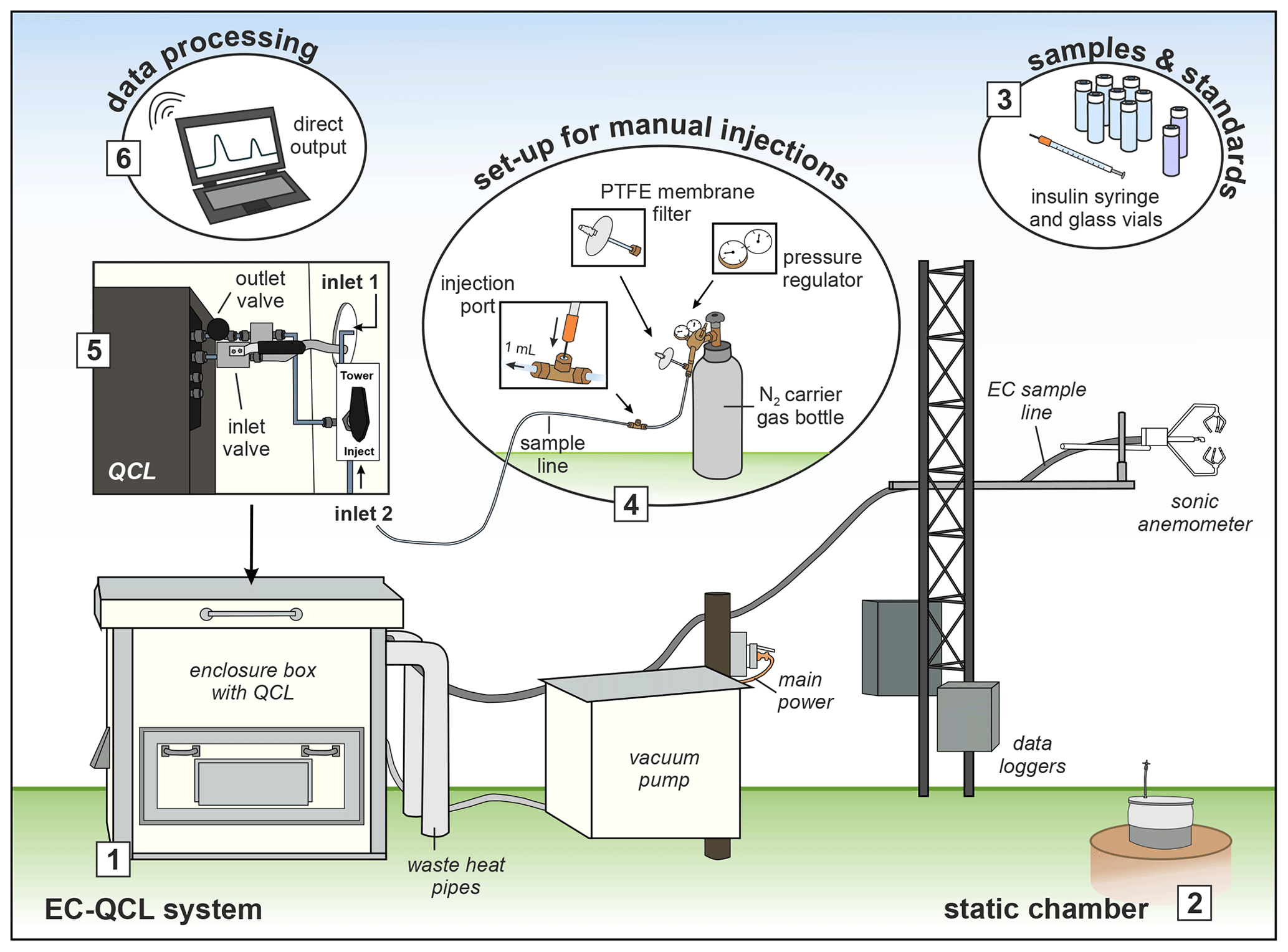
Figure 1Schematic illustration of how to use a field-based QCL for EC measurements and manual injections. (1) The main components of the QCL EC system; (2) an example of a static chamber from which N2O samples were taken and stored in (3) pre-evacuated glass vials. Once the set-up for manual injections (4) was assembled and the QCL air inlet (5) adjusted from drawing ambient air through the EC sample line (inlet 1) to drawing air via the injection tube (inlet 2), the QCL was readily set up to receive injections of N2O samples and associated standards through the injection port. The data output (6) was immediate, allowing processing and data evaluation on the day of chamber sampling.
Once the injection line had been established, the flow rate was reduced from an initial 15 L min−1 used for EC to 1 L min−1 for manual injections based on Savage et al. (2014), Lebegue et al. (2016) and Brümmer et al. (2017). The reduction in flow was monitored using an RMA-SSV flowmeter (Dwyer Instruments, PTY. Ltd., Michigan City, IN, USA) while setting the inlet control valve of the QCL to 2 V (using the TDLWintel software command) before manually adjusting inlet and outlet control valves of the QCL device further until the desired flow rate was achieved. Prior to sample injection, a minimum lag time of 10 min was applied to let the temperature and pressure of the QCL and its temperature-controlled enclosure box return to steady state, i.e. 35 ±0.5 Torr, 33.5 ∘C laser temperature and a QCL enclosure box temperature of 30±0.1 ∘C.
Standards of certified N2O concentration (range 0.2 to 100 ppm) were injected before, during and after each sample run and complemented QCL analysis (Table S2). A total of 10 out of the 12 N2O standards were provided by the NZ-NCNM (except 0.321 and 0.401 ppm) and were therefore identical to those used for GC (Sect. 2.2.2). The QCL measurements were made at 10 Hz frequency with 1 mL of sample air extracted from each sample Exetainer and manually injected into the flow of N2 carrier gas by using a 1 mL glass syringe (SGE International PTY Ltd., VIC, Australia). The glass syringe was flushed with N2 gas after each injection to avoid cross-contamination of samples and N2O standards. The selection of syringe type, flow rate and the usage of N2O standards were based on preliminary tests conducted in advance of the actual field campaign. Finally, it was important to keep a chronological record of the injected sample sequence to allow for a later reidentification of samples in the raw output data from the QCL.
2.3 Data processing
GC and QCL analyses resulted in the output of peak area data from the injected N2O standards and chamber-derived N2O samples (Fig. S1). Data processing therefore first had to determine the relationship between peak area and (known) N2O concentration (CN2O) of the injected standards. To compute the final but initially unknown CN2O of chamber N2O samples, peak area data from N2O standards were fitted to linear and quadratic (second-order polynomial) models (van der Laan et al., 2009; de Klein et al., 2015). de Klein et al. (2015) recommended the use of quadratic curve models as the standard curve for CN2O standards measured by GC analysis. However, we found that both linear and quadratic models adequately fitted CN2O standards derived from QCL. Using a linear fit ultimately resulted in, on average, 3 % smaller FN2O_QCL (range −0.5 % to −4.3 %) than using a quadratic model. Nonetheless, since the quadratic fit suited lower CN2O better than a linear fit, quadratic models were applied to represent the standard curves from injected standards of known CN2O (Fig. S2). The quadratic model used to calculate final CN2O was based on a selection of standards fitted to the expected minimum and maximum range of real samples of CN2O, which in our study ranged between 0.3 and 10 ppm (Fig. S1, Table S2). Output data from GC were processed in PeakSimple software (SRI Instruments, Torrance, CA, USA) and Excel (Microsoft Corp. Redmond, WA, USA). MATLAB R2017a scripting (MathWorks Inc., Natick, MA, USA) served the processing of data derived from the QCL.
2.4 Flux calculation
The FN2O (mg N2O-N m−2 h−1) was calculated for both data streams, GC (FN2O_GC, n=108) and QCL (FN2O_QCL, n=108), by applying a linear regression function to the increase in chamber-headspace CN2O between time t0 and t45 following Eq. (1) (van der Weerden et al., 2011):
where ΔN2O is the increase in headspace CN2O (µL N2O L−1; ppmv) with time, ΔT is the enclosure period (in hours), M is the molar weight of nitrogen in N2O (44 g mol−1), Vm is the molar volume of gas (L mol−1) at the mean air temperature recorded at each sampling occasion, V is the chamber headspace volume (m3), and A is the area covered by the chamber base, here 0.0415 m2. All FN2O was converted to nanomoles of N2O per square metre per second (nmol N2O m−2 s−1) to allow for comparability between GC and QCL outputs. The integration of FN2O_GC (n=84) and FN2O_QCL (n=84) measured at 10:00 sampling was used to quantify the proportion of applied nitrogen emitted as N2O (EN2O) across the 7 d trial in kilograms of N2O-N per hectare (kg N2O-N ha−1) based on Luo et al. (2007) and Wecking et al. (2020a).
2.5 Statistical analyses
The statistical analysis for CN2O data (CN2O_GC and CN2O_QCL, each n=432) and resulting FN2O (FN2O_GC and FN2O_QCL, each n=108) was conducted in Genstat® (Version 19, VSN International, Hemel Hempstead, UK). After testing for normality using a Shapiro–Wilk test and homogeneity of variance by examining residual and fitted values, we applied three different statistical approaches to compare GC with QCL data: (1) orthogonal regression, (2) Bland–Altman and (3) bioequivalence statistics.
The orthogonal regression analysis used standardised CN2O and FN2O data following Eq. (2):
The core of this orthogonal regression was a principal component analysis which, in contrast to ordinary least-squares regression, allowed for measurement errors in the response and the predictor variable by minimising the squared residuals in a vertical and horizontal direction. While orthogonal regression returned a Pearson correlation coefficient r that provided information about the strength of the linear relationship between GC and QCL data, we found that r did not include any prediction about the level of agreement between the two methods (Bland and Altman, 1986; Giavarina, 2015). The degree to which GC and QCL data agreed was, for that reason, determined by using Bland–Altman statistics that quantified the bias (i.e. the mean difference) and the limits of agreement between the two methods. The limits of agreement were calculated from the mean and the standard deviation (SD) of the difference between GC and QCL data, and 95 % of all data points had to be within ±1.96 SD of the mean difference (Giavarina, 2015). The Bland–Altman analysis was conducted for individual FN2O and for mean FN2O across replicates of the same treatment.
Still, testing for correlation and agreement did not determine whether GC and QCL data would effectively and for practical purposes be the same (termed “equivalent”). We therefore used bioequivalence statistics to assess the biological and analytical relevance of the difference between the two methods. The first part of this analysis comprised a one-way analysis of variance (ANOVA) for FN2O, which was subset by treatment (AN0, AN300, AN600, AN900) and analytical device (GC, QCL). Results from this ANOVA determined the 90 % confidence intervals (CIs) of the mean difference between FN2O_QCL and FN2O_GC. In bioequivalence statistics, the 90 % CI (at a standard power level of 80 %) is generally preferred instead of using a 95 % CI that often serves to establish a statistical difference between two methods or treatments rather than proving no difference. An important component of the analysis was to also define the equivalence range, i.e. the maximum acceptable difference, between the new (QCL) and the standard method (GC). Bioequivalence statistics acknowledge that two methods will never be exactly the same. Defining an acceptable equivalence range is thus an important precondition and might in some cases even be provided by a regulatory authority. Originating from pharmaceutical research (Bland and Altman, 1986; Giavarina, 2015; Patterson and Jones, 2006; Rani and Pargal, 2004), the concept of bioequivalence has not broadly been applied in environmental sciences. Therefore, an acceptable equivalence range for N2O data based on the use of different analysers and methods has yet to be defined. We determined that the maximum acceptable difference of FN2O_QCL had to be as small as possible and within ±5 % of the mean difference of the standard method (FN2O_GC). The null hypothesis (FN2O_QCL is different from FN2O_GC) was rejected when the 90 % CI of the difference (FN2O_QCL–FN2O_GC) was entirely within the predefined equivalence range at a significance level of 5 %. Following the same principles, we conducted a bioequivalence analysis for CN2O_QCL and CN2O_GC.
3.1 Environmental conditions and soil variables
Daily mean air temperatures during the 7 d chamber campaign ranged from 8.3 to 12.8 ∘C. The WFPS of the soil within the chambers and associated plots did not fall below 73.9 %, with a mean of 79.5 %. The cumulative rainfall in September 2019 was 119 mm, only 2 mm of which occurred during the 7 d of the campaign. As expected, soil NH and NO levels increased with increasing application of AN fertiliser. The highest values of Nmin measured at AN900 plots were 265 kg NH ha−1 and 268 kg NO ha−1. The mean background levels of soil NH and NO were around 2 kg ha−1. At the end of the campaign, soil NH levels for all treatments had decreased by less than half, while the amount of soil NO remained similar to the initial level measured on the day of treatment application (Table S3).
3.2 Comparing GC- and QCL-derived data
3.2.1 Magnitude and general variability
Measurements resulted in a wide range of FN2O but followed the same temporal and treatment-dependent patterns for both FN2O_GC and FN2O_QCL. The magnitude of individual fluxes was between −0.10 and 22.24 nmol N2O m−2 s−1 for FN2O_GC and −0.07 and 22.81 nmol N2O m−2 s−1 for FN2O_QCL. The mean FN2O (n=27) from chamber plots that received the highest application rate of AN fertiliser (AN900) was 13.22 nmol N2O m−2 s−1 ±1.47 (± standard error of the mean, SEM) for FN2O_GC and 13.27 nmol N2O m−2 s−1 ±1.43 for FN2O_QCL. Similarly, the AN600 treatment had a mean FN2O of 8.51 nmol N2O m−2 s−1 ±0.98 (FN2O_GC) and 8.33 nmol N2O m−2 s−1 ±0.9 (FN2O_QCL). The mean FN2O for AN300 was 6.61 nmol N2O m−2 s−1 ±0.78 (FN2O_GC) and 6.48 nmol N2O m−2 s (FN2O_QCL). At control plots, FN2O values were close to zero (Fig. 2; Table S3). We found that treatment FN2O increased from a near-zero background flux to ≥8.5 nmol N2O m−2 s−1 on the second day of the campaign. From then, AN300 fluxes gradually decreased with time, whereas FN2O at AN600 and AN900 plots remained relatively elevated until the last day of the trial (Fig. 2). These temporal trends aligned with findings from Cowan et al. (2020), who observed N2O emissions to peak within 7 d after urea and AN fertiliser application and found that FN2O returned to background levels after 2 or 3 weeks. Similarly, short-term responses of FN2O to AN application were determined by others, e.g. Bouwman et al. (2002), Jones et al. (2007) and Cardenas et al. (2019). However, for our study, AN treatment effects on FN2O were of secondary interest. Different rates of AN fertiliser were only applied to result in a wide range of CN2O and FN2O (low to high) and thereby allow for comparison of GC and QCL data.

Figure 2Fluxes of nitrous oxide (FN2O) determined from (a) gas chromatography (FN2O_GC) and (b) quantum cascade laser absorption spectrometry (FN2O_QCL). Symbols depict mean FN2O, and marker shading displays the rate of ammonium nitrate (AN) applied: AN0 (black squares), AN300 (dark grey diamonds), AN600 (light grey upside-down triangles) and AN900 (white triangles). Error bars illustrate the standard error of the mean (SEM) across the three replicates of the same treatment. Note that flux measurements on 12 and 15 September were conducted twice daily (10:00 and 12:00) and that the timescale on the x axis is therefore discrete. Soil water-filled pore space (WFPS) and mineral nitrogen (Nmin) contents associated with flux measurements are provided in Table S3.
3.2.2 AN treatment flux and concentration data
The correlation between calculated FN2O_GC and FN2O_QCL and between CN2O_GC and CN2O_QCL across all treatments was high, with an r value of 0.996 resulting from orthogonal regression (Fig. 3a, b). For both cases, major axis as well as ordinary and inverse least squares were nearly identical to a 1:1 line. All three regression models could therefore be used similarly well to predict the strength of the linear relationship between FN2O_GC and FN2O_QCL and between CN2O_GC and CN2O_QCL (Table S4). The results of the orthogonal regression analysis suggested that QCL delivered equivalent data to the GC method. The Bland–Altman statistic quantified a percentage difference between the two methods for FN2O (i.e. FN2O_GC and FN2O_QCL treatment means) of not smaller than −11.2 % and not greater than +9.2 % (Table S5). The percentage difference between individual FN2O_GC and FN2O_QCL (not treatment means) was slightly greater, but it only exceeded +10 % and −15 % in less than 3 % of all cases. This was likely due to the higher variability of FN2O between individual replicates of the same treatment than across calculated means. For both cases, ≥95 % of all data points were well within the predefined limits of agreement ±1.96 SD (Fig. 4b). The overall mean difference (bias) between FN2O_GC and FN2O_QCL was 0.1 nmol N2O m−2 s−1 (Fig. 4b). However, this small bias might be practically irrelevant when compared with the overall detection limit of static chambers and other method-associated uncertainties. Neftel et al. (2007), for instance, quantified the detection limit of static chambers to be 0.23 nmol N2O m−2 s−1, and Parkin et al. (2012) reported 0.03 nmol N2O m−2 s−1. In contrast, Flechard et al. (2007) and others (e.g. Rochette and Eriksen-Hamel, 2008; Jones et al., 2011) showed that the uncertainty of integrated-chamber FN2O can be as high as 50 % at the annual scale.

Figure 3Orthogonal regression analysis of standardised N2O concentrations (CN2O) and fluxes (FN2O). Data were distinguished by their analytic source of origin, i.e. GC (CN2O_GC, FN2O_GC) and QCL (CN2O_QCL, FN2O_QCL). The regression analysis included all CN2O in (a) but only CN2O measured at control sites (AN0) in panel (c). The orthogonal regression analysis was repeated for standardised FN2O, with (b) showing all FN2O_GC and FN2O_QCL and (d) depicting the orthogonal regression for AN0 fluxes only. Ordinary least squares (dotted light grey line) resulted from the regression of Y on X and inverse least squares from the regression of X on Y (long dotted dark grey line). The major axis (black line) based on orthogonal regression of Y and X using a principal component analysis. Here, the squared residuals perpendicular to the line are minimised. Note that for the purpose of illustration axes in panels (c) and (d) have different scales. Table S4 provides further results.
3.2.3 Control flux and concentration data
In contrast to the strong comparability of GC and QCL data at AN treatment sites, FN2O_GC and FN2O_QCL measured at control plots (AN0) were only poorly correlated (r=0.3064) (Fig. 3c). The model fit of the major axis as well as ordinary and inverse least squares indicated that the regression of FN2O_GC on FN2O_QCL (and vice versa) was not identical, i.e. differed in the minimisation of squared residuals in a vertical and horizontal direction. Likewise, this also applied to CN2O_GC and CN2O_QCL (Fig. 3d). Mean FN2O ranged from a minimum of −0.05 to a maximum of only 0.21 nmol N2O m−2 s−1 (Table S3). Consequently, Bland–Altman statistics determined only small quantitative differences between FN2O_GC and FN2O_QCL. When computing the percentage difference between FN2O_GC and FN2O_QCL, we found that near-zero FN2O from AN0 plots were less consistent in relative terms than treatment FN2O (Fig. 4, Table S5). However, these inconsistencies were generally small and did not appear to be of great biological interest.
More generally, QCL analysis resulted in slightly higher CN2O than GC, which explains why the calculated FN2O_QCL values at AN0 plots were higher than FN2O_GC (Table S5). However, whether this finding was related to the potentially higher sensitivity of the QCL device or due to other variations in the sampling procedures was not resolved. Instead, we found that the disagreement between the GC and QCL method was likely related to ambient N2O concentrations in the chamber headspace that remained between 300 and 400 ppb and showed a non-linear response with time, regardless of which analytic device was used. This might have resulted in the calculation of very small but apparent positive and negative FN2O, when in fact the actual flux was zero (Type I error, as defined by Parkin et al., 2012). The integration of CN2O with time to calculate FN2O therefore likely included this error rather than being caused by uncertainties associated with the measurement procedures or choice of analytic device (Kroon et al., 2008). The deviation between control site (AN0) and treatment FN2O (AN300, AN600, AN900) has to be taken into account when evaluating the above results and mathematical principles (Sect. 3.2.2). Furthermore, since static chamber measurements often include near-ambient CN2O, and likewise fluxes equal or near zero, FN2O values from control plots were kept in the paper for completeness.
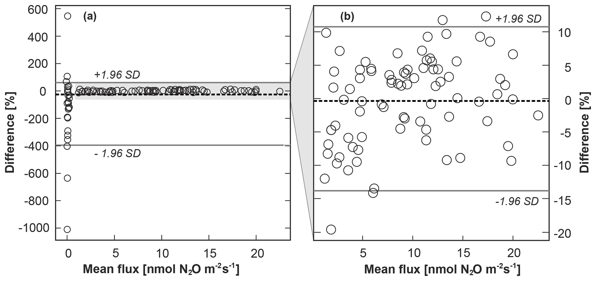
Figure 4Bland–Altman plots showing the difference between the GC and QCL method expressed as the percentage difference of the standard method A (FN2O_GC) and the new method B (FN2O_QCL) on the y axis [((A-B)/mean)×100] versus the mean of A and B on the x axis. The limits of agreement are represented by continuous lines at ±1.96 standard deviation (SD) of the percentage difference. The inset (b) illustrates the same data but excludes FN2O_GC and FN2O_QCL from control (AN0) sites. The percentage mean difference (bias) between FN2O_GC and FN2O_QCL, i.e. method A and B, is indicated by the gap between the dashed line (line of equality, which is not at zero) and an imaginary line parallel to the dashed line at y=0. This figure is based on individual FN2O (all treatment replicates). Results for mean FN2O across replicates of the same treatment are provided in Table S5.
3.2.4 Cumulative N2O emissions
Cumulative N2O emissions across the 7 d campaign were quantified slightly greater for the GC (EN2O_GC) than the QCL (EN2O_QCL) method. The mean difference between EN2O_GC and EN2O_QCL for the control (AN0) and each treatment, AN300, AN600 and AN900, was −0.011, +0.0023, +0.050 and +0.028 kg N ha−1, respectively. This was a difference of less than 4 % in total N2O emissions during deployment (Fig. 5).
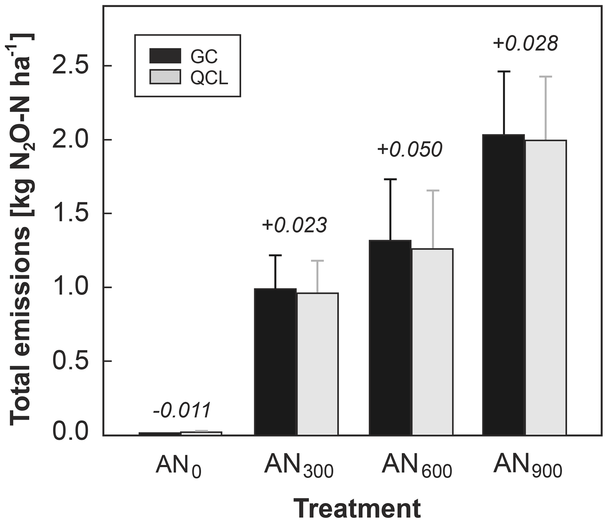
Figure 5Cumulative N2O emissions from each treatment (AN300, AN600, AN900) and the control (AN0) (kg N2O-N ha−1) at the end of the campaign. Data are distinguished into GC (black bars) and QCL (grey bars) budgets. Error bars quantify the standard error of the mean (SEM). The absolute difference (kg N2O-N ha−1) between the two budgets (GC–QCL) is highlighted by the number on top of each pair of bars.
3.3 Measurement performance of QCL analysis
The measurement precision of QCL and, particularly, GC has been generally well-reviewed (de Klein et al., 2015; Lebegue et al., 2016; Rapson and Dacres, 2014). Gas chromatographs can be as precise as <0.5 ppb (van der Laan et al., 2009; Rapson and Dacres, 2014), while the precision of a QCL is about 0.3 ppb for measurements made at 10 Hz and 0.05 ppb for 1 Hz, but in some cases it might be even higher (∼1 ppt) (Curl et al., 2010; Rapson and Dacres, 2014; Savage et al., 2014). Zellweger et al. (2019), for instance, used laboratory QCL for the calibration of N2O reference standards to inform the internationally accepted calibration scale of the Global Atmosphere Watch Programme of the World Meteorological Organisation. Similarly, Rosenstock et al. (2013) verified the accuracy and precision of different photoacoustic spectrometers based on laboratory QCL.
However, the analytic precision can also depend on factors other than the technical performance of the analyser itself. Rannik et al. (2015) indicated that the performance (and thus the precision of FN2O) of an analyser to measure gas samples from a static chamber is likely more limited by the precision of the chamber system than by errors related to the analysis or post-processing of the data. Imprecisions might be caused by several factors, e.g. chamber type and dimensions, experimental set-up, deployment time, and preferred sampling method, all of which can affect the overall flux detection limit (Sect. 3.2.2). In contrast, the sources of uncertainty in our study were most likely related to (1) insufficient evacuation of Exetainers, leading to the sporadic dilution of gas samples and N2O standards, and (2) variation of 1 mL sample volumes when injected into the QCL. In practice, these might not have always been equal to 1 mL and could thus have resulted in slight variations of output peak area. In agreement with our observations, de Klein et al. (2015) found that half the uncertainty of static chamber measurements could be explained by the variability of sample volume in the Exetainers. The inclusion of a fixed-volume sample loop, e.g. when injecting gas samples into the QCL, might help to reduce this source of error in the future.
The QCL analysis of our study was conducted in a temperature- and pressure-controlled environment, where variations in these parameters were unlikely, and the variation in temperature was expected to be less than 0.02 ppb ∘C−1 (Lebegue et al., 2016). Nonetheless, we recommend a constant baseline flow of N2 carrier gas at constant pressure (slightly higher than ambient) and temperature for manual injections made into the QCL device to avoid uncertainty affecting output peak areas. Depending on the QCL EC system, an initial lag time of 10 to 30 min before injections might be required to assemble the operational set-up (Sect. 2.2.3) and ensure sufficient stabilisation of pressure and temperature in the QCL sample cell. Given a flow rate of 1 L min−1, rapid injections into the QCL should become possible shortly afterwards with a delay between single injections of 1 mL sample volumes of not more than 5 to 8 s. Sample concentrations of the same volume but at N2O concentrations >20 ppm required a longer delay time between individual injections (>20 s) to ensure sufficient flushing of the QCL sample cell and avoid cross-contamination (Fig. S1). The identification of suitable delay times was straightforward in our case and could be easily performed in real time by visually examining the peak progression in TDLWintel. When observing the peak progression, for instance, it became noticeable that the injection of blanks (N2 carrier gas) did not result in any changes in baseline flow. However, we did not determine the extent to which spontaneous but small variations in the flow rate of N2 carrier gas would have affected our resulting output peak areas. Further uncertainties might have been associated with processing and curve-fitting procedures applied to the raw dataset in MATLAB and likely resulted in small underestimations of true output peak areas.
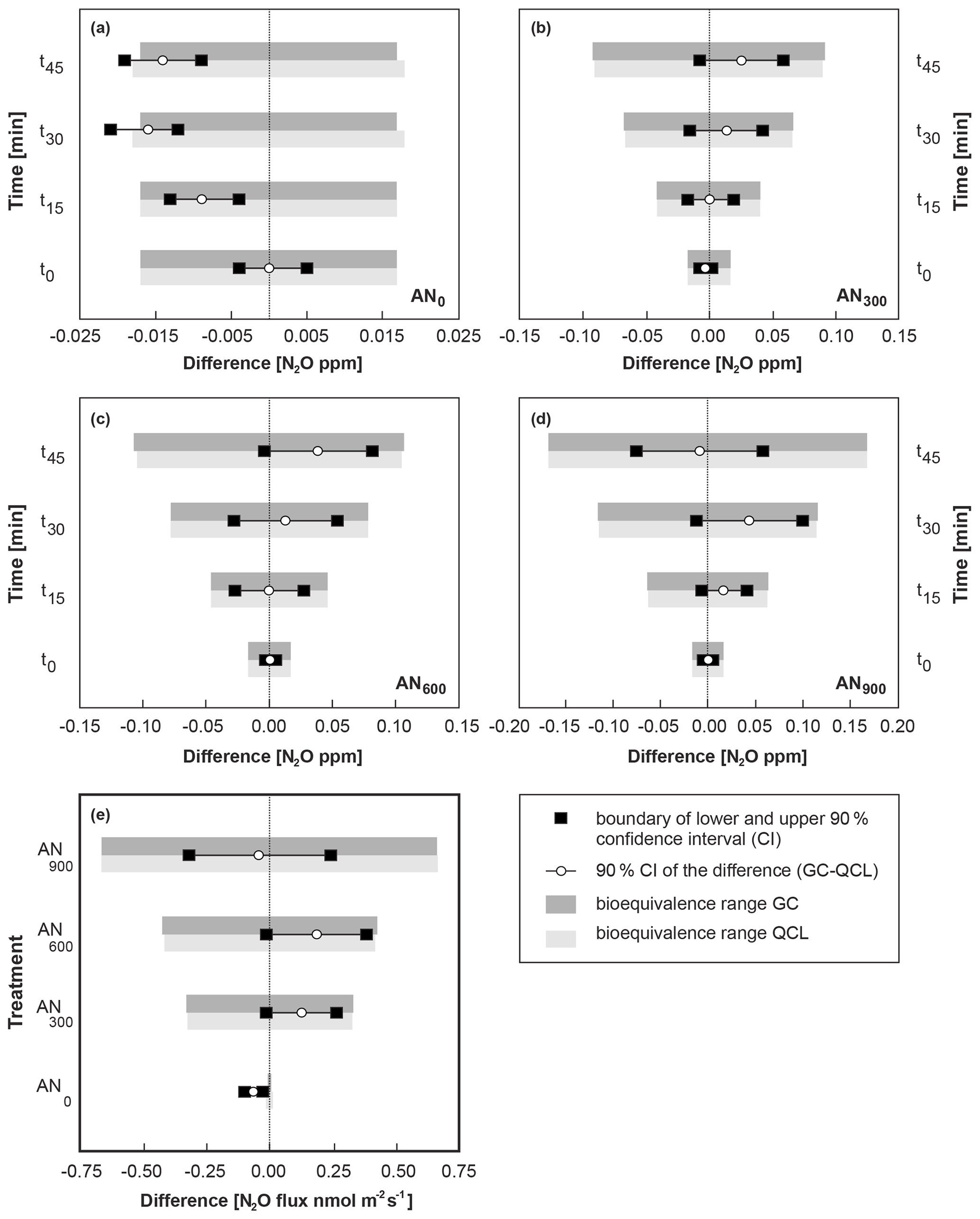
Figure 6Bioequivalence analysis for N2O concentrations (CN2O) in (a–d) and N2O fluxes (FN2O) in (e), with GC defined as the standard method. CN2O and FN2O based on QCL analysis were considered bioequivalent when the 90 % confidence interval (CI) of the difference between QCL and GC (x axis) was completely within the predefined ±5 % bioequivalence range of the difference of the standard method. The bioequivalence analysis was distinguished for CN2O by sampling interval (t0, t15, t30, t45) and treatment, with panel (a) showing results for control sites (AN0) and panels (b), (c) and (d) for AN300, AN600 and AN900 treatment sites. Similarly, a bioequivalence analysis was conducted for FN2O in panel (e) and distinguished by AN application rate on the y axis.
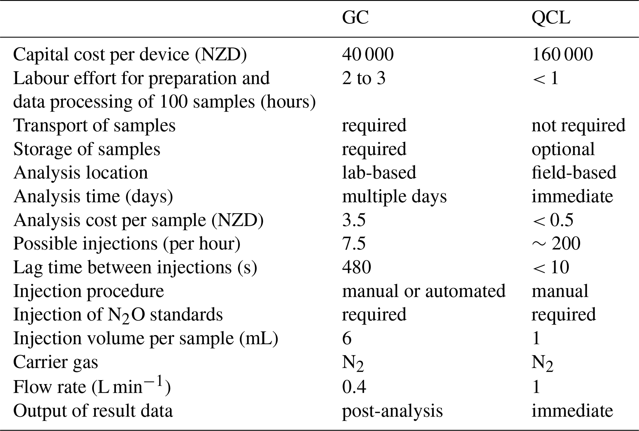
Table 1The GC and QCL methods in comparison: details provided in the table relate to this study, and the information provided was not generalised. NZD: New Zealand dollars.
3.4 QCL injections
3.4.1 The concept of bioequivalence
Using the Pearson correlation coefficient and the coefficient of determination for comparing two or more quantitative methods is a generally preferred approach in the field of N2O research. Comparisons of different methods for N2O analysis made in the literature most commonly use orthogonal (Jones et al., 2011) and linear regression (Cowan et al., 2014; Brümmer et al., 2017; Tallec et al., 2019), Student's t tests (Christiansen et al., 2015), or are based on raw data (Savage et al., 2014). However, correlation studies as such have limitations when assessing the comparability between two methods since a correlation analysis only identifies the relationship between two variables, not the difference (Giavarina, 2015). Bland–Altman and bioequivalence statistics overcome this limitation by assessing the degree of agreement between methods.
An important aspect of statistical hypothesis testing is that the null hypothesis is never accepted. But failure to reject the null hypothesis is not the same as proving no difference. A bioequivalence analysis allows the statistical assessment of whether two methods (e.g. measurement devices, drug treatment) are effectively the same. Central to a bioequivalence analysis is the “equivalence range” that defines the size of the acceptable difference for which the values are similar enough to be considered equivalent. This becomes important when considering that even with the most precise analytical design and the most tightly controlled experimental conditions, e.g. FN2O_GC and FN2O_QCL will never be exactly the same (Rani and Pargal, 2004). However, if the difference is sufficiently small for “practical purposes”, FN2O_GC and FN2O_QCL can be considered effectively the same. Here, accepted evidence of bioequivalence for FN2O_QCL was that the 90 % confidence interval of the difference FN2O_QCL–FN2O_GC (corresponding to a test with size 0.05) was within a ±5 % difference of FN2O_GC. The equivalence range will vary depending on the objective of the research or guidelines provided by a regulatory authority, but it commonly does not exceed ±20 % (Westlake, 1988; Rani and Pargal, 2004; Ring et al., 2019). In our study, a small equivalence range of ±5 % was preferred to test the difference between FN2O_QCL and FN2O_GC since such recommendations did not exist.
Overall, our results showed that FN2O_GC and FN2O_QCL from AN300, AN600 and AN900 plots provided evidence of bioequivalence. The 90 % confidence intervals of the difference (FN2O_GC–FN2O_QCL) were quantified at 0.127 (AN300), 0.185 (AN600) and −0.043 nmol N2O m−2 s−1 (AN900) and are well within the predefined equivalence range of ±5 % (Fig. 6e, Table S6). At control sites (AN0), FN2O_GC and FN2O_QCL did not provide evidence for bioequivalence. However, the failure to establish equivalence for AN0 sites was due to the overall limitation of the static chamber method to provide “real” FN2O, rather than based on a failure of the statistical principle (Sect. 3.2.3). In contrast, when tested for CN2O instead of FN2O, equivalence was confirmed for t0 and t15 but did not apply to t30 and t45 (Fig. 6a). Again, failure to establish equivalence was likely related to limitations of the static chamber method, which, in this case, were indicated by the lower boundary of the 90 % CI remaining outside the predefined equivalence ranges. Another possible reason for not accepting equivalence for GC- and QCL-derived data at AN0 sites could have been the maximum acceptable difference between the two methods. We defined (Sect. 2.5) this difference as having to be within ±5 % of the mean difference of the standard method (i.e. GC). It has to be taken into consideration that the accepted evidence of bioequivalence would have led to different results if the percentage mean difference had been set to, for instance, ±10 %. Accepting a greater mean difference between the two methods would have consequently resulted in evidencing bioequivalence for CN2O_GC and CN2O_QCL even at ambient concentrations. More generally, we found that positive values of the 90 % CI of the difference indicated that the difference between the two methods (GC–QCL) resulted in higher CN2O_GC and FN2O_GC. Negative values instead showed that the difference GC–QCL led CN2O_QCL and FN2O_QCL values to be greater than those from CN2O_GC and FN2O_GC, but in either case, the overall difference between the two methods did not exceed ±0.1 ppm for CN2O and ±0.38 nmol N2O m−2 s−1 for FN2O (Fig. 6e).
To the best of our knowledge, bioequivalence has not been broadly applied in the greenhouse gas literature to identify and discuss the range at which a difference in FN2O_GC and FN2O_QCL could be considered relevant when using different analytical methods. However, defining the magnitude of FN2O (e.g. in nmol N2O m−2 s−1) at which a unit difference would become relevant is important when using different methods to quantify, compare and, ultimately, upscale N2O emissions. We thus recommend bioequivalence or other statistical approaches (e.g. Bland–Altman statistics) for more formally assessing the agreement between two methods in the future.
3.4.2 Strengths and weaknesses
The employment of a QCL analyser proposes an alternative approach for the injection of N2O samples taken from static chambers, particularly as FN2O_QCL values were generally equivalent to FN2O_GC. Using a QCL for manual injections can be conducted without much disruption to other measurements (e.g. EC or automated chambers) and therefore helps justify the initially higher capital and general running costs involved with operating a QCL device. Additional labour effort and time associated with sample storage and transport necessary for laboratory GC do not necessarily apply for field-based injections into a QCL. Once established, a QCL system has relatively low maintenance and offers a straightforward application for manual injections in addition to EC or other measurement tasks. In our study, the assembly of the injection set-up required little equipment and was installed within 30 min. This allowed for a rapid analysis after chamber sampling without greatly interfering with other measurements, i.e. EC, that were offline during the time of injection into the QCL. To collectively inject a great number of samples turned out to be highly beneficial to minimise the downtime of the EC measurements in our case, and it also helped to reduce other interferences made to the QCL. For instance, we were able to inject a total of around 700 1 mL samples (432 samples, 268 standards) within 4 h (Table 1). Prior to QCL analysis, these samples had been kept in septum-sealed Exetainers that can store gas samples for up to 28 d at any temperature between −10 and 25 ∘C (Faust and Liebig, 2018). We acknowledge that a sporadic dilution of our samples might still have occurred due to storage in and potentially insufficient evacuation of Exetainers, which, in turn, could have affected subsequent GC and QCL analyses (de Klein et al., 2015). Despite this potential source of uncertainty, storing N2O samples in Exetainers enabled repeated injections and allowed us to postpone the analysis if EC measurements were of higher importance or if the weather conditions (e.g. precipitation) were unsuitable. Similar to GC, QCL injections required consumables (N2 carrier gas, N2O standards) but, in contrast, time and costs associated with laboratory work were substantially less (Table 1).
Previously, QCL had been used either in conjunction with EC or coupled to automated chambers. Here, we showed that one QCL device could be used as a practical tool for the analysis of static-chamber-derived N2O samples without major disruption to these other measurement tasks. We found that treatment N2O concentrations (CN2O_QCL) and fluxes (FN2O_QCL) from QCL agreed with results based on laboratory GC (CN2O_GC, FN2O_GC). The percentage difference between treatment FN2O_GC and FN2O_QCL was not smaller than −11.2 % and not greater than +9.2 %, with a mean difference between the two of only 0.1 nmol N2O m−2 s−1. A deviation between the GC and QCL methods was determined only for close-to-zero FN2O at control plots where FN2O_GC and FN2O_QCL values were found outside the predefined equivalence range. However, this was likely due to the calculation of very small but apparent positive and negative FN2O (when in fact the actual flux was zero), rather than due to uncertainties caused by a weakness of the GC or QCL analysis. Equivalence was evidenced for all other FN2O_GC and FN2O_QCL and confirmed that GC and QCL data were for practical purposes the same. We found that using Bland–Altman and bioequivalence statistics in addition to regression analysis served the comparison of GC and QCL particularly well. Yet, these two statistical approaches have not been broadly used in the field of greenhouse gas research to compare different analytical methods or to discuss the magnitude at which a difference in FN2O would become relevant. Since correlation studies identify the relationship between two methods but not the difference, we recommend that bioequivalence or other suitable statistical approaches be used for more formally assessing the agreement between two methods. Finally, QCL offers great potential to interlink different methods of gas measurements across different temporal and spatial scales. In the future, this capability might be important not only for rapid field analysis of N2O samples but might also equally apply to the measurement of other gas species (e.g. CO2, CH4) and gas isotopomers of interest.
Data were deposited at the University of Waikato Research Commons; see https://researchcommons.waikato.ac.nz/handle/10289/13539 (last access: 4 September 2020, Wecking et al., 2020b).
The supplement related to this article is available online at: https://doi.org/10.5194/amt-13-5763-2020-supplement.
ARW, VMC, JL and LAS designed the experiment. ARW performed the fieldwork. ARW conducted the post-processing of GC and QCL data using MATLAB scripts, which are based on the work of ARW and DIC. ARW performed the statistical analysis with inputs and contributions from VMC. VMC and LAS commented on the results of the initial data analysis. ARW wrote and revised the paper with contributions from VMC, ARW, LLL, JL, DIC and LAS.
The authors declare that they have no conflict of interest.
The authors would like to recognise the farm owners, Sarah and Ben Troughton, for their cooperation. Chris Morcom is thanked for his help in the fields and Emily Huang from NZ-NCNM for her all-embracing support regarding gas chromatography. Training notes on the concept of bioequivalence were gratefully received from Neil Cox. We would like to further acknowledge continuous support from Aerodyne Research Ltd. in maintaining and advancing our QCL EC systems. Finally, Cecile A. M. de Klein, Jordan P. Goodrich, Tom P. Moore and two anonymous reviewers are thanked for thoroughly revising this paper.
This research project (grant nos. 17-CAN9.3.4, 19-CAN9.8) was supported by the New Zealand Agricultural Greenhouse Gas Research Centre (NZAGRC), AgResearch Ruakura, DairyNZ and the University of Waikato.
This paper was edited by Daniela Famulari and reviewed by two anonymous referees.
Baldocchi, D.: Measuring fluxes of trace gases and energy between ecosystems and the atmosphere – the state and future of the eddy covariance method, Global Change Biol., 20, 3600–3609, https://doi.org/10.1111/gcb.12649, 2014.
Bland, M. J. and Altman, D. G.: Statistical method for assessing agreement between two methods of clinical measurement, The Lancet, 327, 307–310, https://doi.org/10.1016/S0140-6736(86)90837-8, 1986.
Bouwman, A. F., Boumans, L. J. M., and Batjes, N. H.: Emissions of N2O and NO from fertilized fields: Summary of available measurement data, Global Biogeochem. Cy., 16, 6–1, 2002.
Brümmer, C., Lyshede, B., Lempio, D., Delorme, J.-P., Rüffer, J. J., Fuß, R., Moffat, A. M., Hurkuck, M., Ibrom, A., Ambus, P., Flessa, H., and Kutsch, W. L.: Gas chromatography vs. quantum cascade laser-based N2O flux measurements using a novel chamber design, Biogeosciences, 14, 1365–1381, https://doi.org/10.5194/bg-14-1365-2017, 2017.
Butterbach-Bahl, K., Baggs, E. M., Dannenmann, M., Kiese, R., and Zechmeister-Boltenstern, S.: Nitrous oxide emissions from soils: how well do we understand the processes and their controls?, Philos. Trans. Roy. Soc. London B, 368, 20130122, https://doi.org/10.1098/rstb.2013.0122, 2013.
Cardenas, L. M., Bhogal, A., Chadwick, D. R., McGeough, K., Misselbrook, T., Rees, R. M., Thorman, R. E., Watson, C. J., Williams, J. R., Smith, K. A., and Calvet, S.: Nitrogen use efficiency and nitrous oxide emissions from five UK fertilised grasslands. Sci. Total Environ. 661, 696–710, https://doi.org/10.1016/j.scitotenv.2019.01.082, 2019.
Chadwick, D. R., Cardenas, L., Misselbrook, T. H., Smith, K. A., Rees, R. M., Watson, C. J., McGeough, K. L., Williams, J. R., Cloy, J. M., Thorman, R. E., and Dhanoa, M. S.: Optimizing chamber methods for measuring nitrous oxide emissions from plot-based agricultural experiments, Eur. J. Soil Sci., 65, 295–307, https://doi.org/10.1111/ejss.12117, 2014.
Christiansen, J. R., Korhonen, J. F. J., Juszczak, R., Giebels, M., and Pihlatie, M.: Assessing the effects of chamber placement, manual sampling and headspace mixing on CH4 fluxes in a laboratory experiment, Plant Soil, 343, 171–185, https://doi.org/10.1007/s11104-010-0701-y, 2011.
Christiansen, J. R., Outhwaite, J., and Smukler, S. M.: Comparison of CO2, CH4 and N2O soil-atmosphere exchange measured in static chambers with cavity ring-down spectroscopy and gas chromatography, Agr. Forest Meteorol., 211–212, 48–57, https://doi.org/10.1016/j.agrformet.2015.06.004, 2015.
Cowan, N., Levy, P., Maire, J., Coyle, M., Leeson, S. R., Famulari, D., Carozzi, M., Nemitz, E., and Skiba, U.: An evaluation of four years of nitrous oxide fluxes after application of ammonium nitrate and urea fertilisers measured using the eddy covariance method, Agr. Forest Meteorol., 280, 107812, https://doi.org/10.1016/j.agrformet.2019.107812, 2020.
Cowan, N. J., Famulari, D., Levy, P. E., Anderson, M., Bell, M. J., Rees, R. M., Reay, D. S., and Skiba, U. M.: An improved method for measuring soil N2O fluxes using a quantum cascade laser with a dynamic chamber, Eur. J. Soil Sci., 65, 643–652, https://doi.org/10.1111/ejss.12168, 2014.
Curl, R. F., Capasso, F., Gmachl, C., Kosterev, A. A., McManus, B., Lewicki, R., Pusharsky, M., Wysocki, G., and Tittel, F. K.: Quantum cascade lasers in chemical physics, Chem. Phys. Lett., 487, 1–18, https://doi.org/10.1016/j.cplett.2009.12.073, 2010.
de Klein, C. A. M., Barton, L., Sherlock, R. R., Li, Z., and Littlejohn, R. P.: Estimating a nitrous oxide emission factor for animal urine from some New Zealand pastoral soils, Aust. J. Soil Res., 41, 381–399, https://doi.org/10.1071/SR02128, 2003.
de Klein, C. A. M., Harvey, M. J., Clough, T., Rochette, P., Kelliher, F., Venetera, R., Alfaro, M., and Chadwick, D.: Nitrous Oxide Chamber Methodology Guidelines. Version 1.1, Ministry of Primary Industries, Wellington, 146, 2015.
Denmead, O.: Approaches to measuring fluxes of methane and nitrous oxide between landscapes and the atmosphere, Plant Soil, 309, 5–24, https://doi.org/10.1007/s11104-008-9599-z, 2008.
Erisman, J. W., Galloway, J. N., Seitzinger, S., Bleeker, A., Dise, N. B., Petrescu, A. M. R., Leach, A. M., and de Vries, W.: Consequences of human modification of the global nitrogen cycle, Philos. Trans. Roy. Soc. B, 368, 1–9, https://doi.org/10.1098/rstb.2013.0116, 2013.
Faust, D. R. and Liebig, M. A.: Effects of storage time and temperature on greenhouse gas samples in Exetainer vials with chlorobutyl septa caps, MethodsX, 5, 857–864, https://doi.org/10.1016/j.mex.2018.06.016, 2018.
Firestone, M. K. and Davidson, E. A.: Microbiological Basis of NO and N2O Production and Consumption in Soil, in: Exchange of Trace Gases between Terrestrial Ecosystems and the Atmosphere, edited by: Andreae, M. O., and Schmimmel, D. S., John Wiley & Sons Ltd, 7–21, 1989.
Flechard, C. R., Ambus, P., Skiba, U., Rees, R. M., Hensen, A., van Amstel, A., van Den Pol-van Dasselaar, A., Soussana, J. F., Jones, M., Clifton-Brown, J., Raschi, A., Horvath, L., Neftel, A., Jocher, M., Ammann, C., Leifeld, J., Fuhrer, J., Calanca, P., Thalman, E., Pilegaard, K., Di Marco, C., Campbell, C., Nemitz, E., Hargreaves, K. J., Levy, P. E., Ball, B. C., Jones, S. K., van de Bulk, W. C. M., Groot, T., Blom, M., Domingues, R., Kasper, G., Allard, V., Ceschia, E., Cellier, P., Laville, P., Henault, C., Bizouard, F., Abdalla, M., Williams, M., Baronti, S., Berretti, F., and Grosz, B.: Effects of climate and management intensity on nitrous oxide emissions in grassland systems across Europe, Agr. Ecosyst. Environ., 121, 135–152, https://doi.org/10.1016/j.agee.2006.12.024, 2007.
Giavarina, D.: Understanding Bland Altman analysis, Biochem. Medica, 25, 141–151, https://doi.org/10.11613/BM.2015.015, 2015.
Hewitt, A. E.: New Zealand Soil Classification, 2nd Edn., Manaaki-Whenua Press, Lincoln, New Zealand, 2010.
Hutchinson, G. L. and Mosier, A. R.: Improved Soil Cover Method for Field Measurement of Nitrous Oxide Fluxes1, Soil Sci. Soc. Am. J., 45, 311–316, https://doi.org/10.2136/sssaj1981.03615995004500020017x, 1981.
IPCC: Anthropogenic and Natural Radiative Forcing, in: Climate Change 2013: The Physical Science Basis. Contribution of Working Group I to the Fifth Assessment Report of the Intergovenmental Panel on Climate Change., edited by: Myhre, G., Shindell, D., Breon, F.-M., Collins, W., Fuglestvedt, J., Huang, J., Koch, D., Lamarque, J.-F., Lee, D., Mendoza, B., Nakajima, T., Robock, A., Stephens, G., Takemura, T., Zhang, H., Jacob, D., Ravishankara, A. R., and Shine, K. P., Cambidge UK and New York, NY, USA, 659–740, 2013.
Jones, S. K., Famulari, D., Di Marco, C. F., Nemitz, E., Skiba, U. M., Rees, R. M., and Sutton, M. A.: Nitrous oxide emissions from managed grassland: a comparison of eddy covariance and static chamber measurements, Atmos. Meas. Tech., 4, 2179–2194, https://doi.org/10.5194/amt-4-2179-2011, 2011.
Jones, S. K., Rees, R. M., Skiba, U. M., and Ball, B. C.: Influence of organic and mineral N fertiliser on N2O fluxes from a temperate grassland, Agr. Ecosyst. Environ., 121, 74–83, https://doi.org/10.1016/j.agee.2006.12.006, 2007.
Kroon, P., Hensen, A., Bulk, W., Jongejan, P., and Vermeulen, A.: The importance of reducing the systematic error due to non-linearity in N2O flux measurements by static chambers, Nutr. Cycling Agroecosyst., 82, 175–186, https://doi.org/10.1007/s10705-008-9179-x, 2008.
Lammirato, C., Lebender, U., Tierling, J., and Lammel, J.: Analysis of uncertainty for N2O fluxes measured with the closed-chamber method under field conditions: Calculation method, detection limit, and spatial variability, J. Plant Nutr. Soil Sci., 181, 78–89, https://doi.org/10.1002/jpln.201600499, 2018.
Lebegue, B., Schmidt, M., Ramonet, M., Wastine, B., Yver Kwok, C., Laurent, O., Belviso, S., Guemri, A., Philippon, C., Smith, J., and Conil, S.: Comparison of nitrous oxide (N2O) analyzers for high-precision measurements of atmospheric mole fractions, Atmos. Meas. Tech., 9, 1221–1238, https://doi.org/10.5194/amt-9-1221-2016, 2016.
Liáng, L. L., Campbell, D. I., Wall, A. M., and Schipper, L. A.: Nitrous oxide fluxes determined by continuous eddy covariance measurements from intensively grazed pastures: Temporal patterns and environmental controls, Agr. Ecosyst. Environ., 268, 171–180, https://doi.org/10.1016/j.agee.2018.09.010, 2018.
Lundegard, H.: Carbon dioxide evolution of soil and crop growth, Soil Sci., 23, 417–453, 1927.
Luo, J., Ledgard, S. F., and Lindsey, S. B.: Nitrous oxide emissions from application of urea on New Zealand pasture, N. Z. J. Agric. Res., 50, 1–11, https://doi.org/10.1080/00288230709510277, 2007.
Luo, J., Ledgard, S., Klein, C., Lindsey, S., and Kear, M.: Effects of dairy farming intensification on nitrous oxide emissions, Plant Soil, 309, 227–237, https://doi.org/10.1007/s11104-007-9444-9, 2008a.
Luo, J., Lindsey, S., and Ledgard, S.: Nitrous oxide emissions from animal urine application on a New Zealand pasture, Biol. Fertil. Soils, 44, 463–470, https://doi.org/10.1007/s00374-007-0228-4, 2008b.
Luo, J., Wyatt, J., van der Weerden, T. J., Thomas, S. M., de Klein, C. A. M., Li, Y., Rollo, M., Lindsey, S., Ledgard, S. F., Li, J., Ding, W., Qin, S., Zhang, N., Bolan, N. S., Kirkham, M. B., Bai, Z., Ma, L., Zhang, X., Wang, H., Liu, H., and Rys, G.: Potential Hotspot Areas of Nitrous Oxide Emissions From Grazed Pastoral Dairy Farm Systems, Adv. Agro., 145, 205–268, https://doi.org/10.1016/bs.agron.2017.05.006, 2017.
Mulvaney, R. L.: Extraction of exchangeable ammonium, nitrate and nitrite, in: Methods of soil analysis Part 3: chemical methods, edited by: Sparks, D. L., Page, A. L., Helmke, P. A., and Loeppert, R. H., 5.3, Soil Sci. Soc. Am., American Society of Agronomy, Madison, WI, 1129–1131, 1996.
Neftel, A., Flechard, C., Ammann, C., Conen, F., Emmenegger, L., and Zeyer, K.: Experimental assessment of N2O background fluxes in grassland systems, Tellus B, 59, 470–482, https://doi.org/10.1111/j.1600-0889.2007.00273.x, 2007.
Nelson, D. D., McManus, B., Urbanski, S., Herndon, S., and Zahniser, M. S.: High precision measurements of atmospheric nitrous oxide and methane using thermoelectrically cooled mid-infrared quantum cascade lasers and detectors, Spectrochim. Acta, Part A, 60, 3325–3335, https://doi.org/10.1016/j.saa.2004.01.033, 2004.
Nemitz, E., Mammarella, I., Ibrom, A., Aurela, M., Burba, G., Dengel, S., Gielen, B., Grelle, A., Heinesch, B., Herbst, M., Hörtnagl, L., Klemedtsson, L., Lindroth, A., Lohila, A., McDermitt, K. D., Meier, P., Merbold, L., Nelson, D., Nicolini, G., and Zahniser, M.: Standardisation of eddy-covariance flux measurements of methane and nitrous oxide, Int. Agrophys., 32, 517–549, https://doi.org/10.1515/intag-2017-0042, 2018.
Nicolini, G., Castaldi, S., Fratini, G., and Valentini, R.: A literature overview of micrometeorological CH4 and N2O flux measurements in terrestrial ecosystems, Atmos. Environ., 81, 311–319, https://doi.org/10.1016/j.atmosenv.2013.09.030, 2013.
NIWA: National Climate Database, National Institute of Water and Atmospheric Research, available at: http://cliflo.niwa.co.nz/ (last access: 4 September 2020), 2018.
Parkin, T. B. and Venterea, R. T.: USDA-ARS GRACEnet Project Protocols Sampling Protocols. Chamber-Based Trace Gas Flux Measurements, in: Sampling Protocols, edited by: Follett, R. F., U.S. Department of Agriculture, Agricultural Research Service, National Laboratory for Agriculture & the Environment, Ames, IA, St. Paul, MN, 3.1–3.39, chapter 3, available at: https://www.ars.usda.gov/natural-resources-and-sustainable-agricultural-systems/soil-and-air/docs/gracenet-sampling-protocols/, last access: 28 October 2010.
Parkin, T. B., Venterea, R. T., and Hargreaves, S. K.: Calculating the Detection Limits of Chamber-based Soil Greenhouse Gas Flux Measurements, J. Environ. Qual., 41, 705–715, https://doi.org/10.2134/jeq2011.0394, 2012.
Patterson, S. and Jones, B.: Interdisciplinary statistics. Bioequivalence and statistics in clinical pharmacology, Taylor & Francis Group, Boca Raton, FL, 2006.
Pavelka, M., Acosta, M., Kiese, R., Altimir, N., Bruemmer, C., Crill, P., Darenova, E., Fuß, R., Gielen, B., Graf, A., Klemedtsson, L., Lohila, A., Longdoz, B., Lindroth, A., Nilsson, M., Marañón-Jiménez, S., Merbold, L., Montagnani, L., Peichl, M., and Kutsch, W. L.: Standardisation of chamber technique for CO2, N2O and CH4 fluxes measurements from terrestrial ecosystems, Int. Agrophys., 32, 569–587, https://doi.org/10.1515/intag-2017-0045, 2018.
Rani, S. and Pargal, A.: Bioequivalence: An overview of statistical concepts, Indian J. Pharm., 36, 209–216, 2004.
Rannik, Ü., Haapanala, S., Shurpali, N. J., Mammarella, I., Lind, S., Hyvönen, N., Peltola, O., Zahniser, M., Martikainen, P. J., and Vesala, T.: Intercomparison of fast response commercial gas analysers for nitrous oxide flux measurements under field conditions, Biogeosciences, 12, 415–432, https://doi.org/10.5194/bg-12-415-2015, 2015.
Rapson, T. D. and Dacres, H.: Analytical techniques for measuring nitrous oxide, “TrAC, Trends Anal. Chem.”, 54, 65–74, https://doi.org/10.1016/j.trac.2013.11.004, 2014.
Ravishankara, J. S., Daniel, R. W., and Portmann, R. W.: Nitrous oxide (N2O): The dominant ozone-depleting substance emitted in the 21st century, Science, 326, 123–125, https://doi.org/10.1126/science.1176985, 2009.
Reay, D. S., Davidson, E. A., Smith, K. A., Smith, P., Melillo, J. M., Dentener, F., and Crutzen, P. J.: Global agriculture and nitrous oxide emissions, Nat. Clim. Change, 2, 410–416, https://doi.org/10.1038/nclimate1458, 2012.
Rees, R. M., Augustin, J., Alberti, G., Ball, B. C., Boeckx, P., Cantarel, A., Castaldi, S., Chirinda, N., Chojnicki, B., Giebels, M., Gordon, H., Grosz, B., Horvath, L., Juszczak, R., Kasimir Klemedtsson, Å., Klemedtsson, L., Medinets, S., Machon, A., Mapanda, F., Nyamangara, J., Olesen, J. E., Reay, D. S., Sanchez, L., Sanz Cobena, A., Smith, K. A., Sowerby, A., Sommer, M., Soussana, J. F., Stenberg, M., Topp, C. F. E., van Cleemput, O., Vallejo, A., Watson, C. A., and Wuta, M.: Nitrous oxide emissions from European agriculture – an analysis of variability and drivers of emissions from field experiments, Biogeosciences, 10, 2671–2682, https://doi.org/10.5194/bg-10-2671-2013, 2013.
Ring, A., Lang, B., Kazaroho, C., Labes, D., Schall, R., and Schütz, H.: Sample size determination in bioequivalence studies using statistical assurance, Brit. J. Clin. Pharmaco., 85, 2369–2377, https://doi.org/10.1111/bcp.14055, 2019.
Rochette, P. and Bertrand, N.: Soil air sample storage and handling using polypropylene syringes and glass vials, Can. J. Soil Sci., 83, 631–637, https://doi.org/10.4141/S03-015, 2003.
Rochette, P. and Eriksen-Hamel, N.: Chamber Measurements of Soil Nitrous Oxide Flux: Are Absolute Values Reliable?, Soil Sci. Soc. Am. J., 72, 331–342, https://doi.org/10.2136/sssaj2007.0215, 2008.
Rochette, P.: Towards a standard non-steady-state chamber methodology for measuring soil N2O emissions, Anim. Feed Sci. Technol., 166, 141–146, https://doi.org/10.1016/j.anifeedsci.2011.04.063, 2011.
Rosenstock, T. S., Diaz-Pines, E., Zuazo, P., Jordan, G., Predotova, M., Mutuo, P., Abwanda, S., Thiong'o, M., Buerkert, A., Rufino, M. C., Kiese, R., Neufeldt, H., and Butterbach-Bahl, K.: Accuracy and precision of photoacoustic spectroscopy not guaranteed, Global Change Biol., 19, 3565–3567, https://doi.org/10.1111/gcb.12332, 2013.
Savage, K., Phillips, R., and Davidson, E.: High temporal frequency measurements of greenhouse gas emissions from soils, Biogeosciences, 11, 2709–2720, https://doi.org/10.5194/bg-11-2709-2014, 2014.
Selbie, D. R., Buckthought, L. E., and Shepherd, M. A.: Chapter Four – The Challenge of the Urine Patch for Managing Nitrogen in Grazed Pasture Systems, Adv. Agron., 129, 229–292, https://doi.org/10.1016/bs.agron.2014.09.004, 2015.
Tallec, T., Brut, A., Joly, L., Dumelié, N., Serça, D., Mordelet, P., Claverie, N., Legain, D., Barrié, J., Decarpenterie, T., Cousin, J., Zawilski, B., Ceschia, E., Guérin, F., and Le Dantec, V.: N2O flux measurements over an irrigated maize crop: A comparison of three methods, Agr. Forest. Meteorol., 264, 56–72, https://doi.org/10.1016/j.agrformet.2018.09.017, 2019.
Thompson, R. L., Lassaletta, L., Patra, P. K., Wilson, C., Wells, K. C., Gressent, A., Koffi, E. N., Chipperfield, M. P., Winiwarter, W., Davidson, E. A., Tian, H., and Canadell, J. G.: Acceleration of global N2O emissions seen from two decades of atmospheric inversion, Nat. Clim. Change, 9, 1–6, https://doi.org/10.1038/s41558-019-0613-7, 2019.
van der Laan, S., Neubert, R. E. M., and Meijer, H. A. J.: A single gas chromatograph for accurate atmospheric mixing ratio measurements of CO2, CH4, N2O, SF6 and CO, Atmos. Meas. Tech., 2, 549–559, https://doi.org/10.5194/amt-2-549-2009, 2009.
van der Weerden, T. J., Luo, J., de Klein, C. A. M., Hoogendoorn, C. J., Littlejohn, R. P., and Rys, G. J.: Disaggregating nitrous oxide emission factors for ruminant urine and dung deposited onto pastoral soils, Agr. Ecosyst. Environ., 141, 426–436, https://doi.org/10.1016/j.agee.2011.04.007, 2011.
van der Weerden, T. J., Clough, T. J., and Styles, T. M.: Using near-continuous measurements of N2O emission from urine-affected soil to guide manual gas sampling regimes, N. Z. J. Agric. Res., 56, 60–76, https://doi.org/10.1080/00288233.2012.747548, 2013.
Velthof, G. L., Jarvis, S. C., Stein, A., Allen, A. G., and Oenema, O.: Spatial variability of nitrous oxide fluxes in mown and grazed grasslands on a poorly drained clay soil, Soil Biol. Biochem., 28, 1215–1225, https://doi.org/10.1016/0038-0717(96)00129-0, 1996.
Wecking, A. R., Wall, A. M., Liáng, L. L., Lindsey, S. B., Luo, J., Campbell, D. I., and Schipper, L. A.: Reconciling annual nitrous oxide emissions of an intensively grazed dairy pasture determined by eddy covariance and emission factors, Agr. Ecosyst. Environ., 287, 106646, https://doi.org/10.1016/j.agee.2019.106646, 2020a.
Wecking, A. R., Cave, V. M., Liáng, L. L., Wall, A. M., Luo, J., Campbell, D. I., and Schipper, L. A.: Dataset for “A novel injection technique: using a field-based quantum cascade laser for the analysis of gas samples derived from static chamber”, University of Waikato, available at: https://researchcommons.waikato.ac.nz/handle/10289/13539, last access: 4 September 2020b.
Westlake, W. J.: Bioavailability and bioequivalence of pharmaceutical formulations, in: Biopharmaceutical Statistics for Drug Development, edited by: Peace, K. E., Marcel Dekker, New York, 329–352, 1988.
Zellweger, C., Steinbrecher, R., Laurent, O., Lee, H., Kim, S., Emmenegger, L., Steinbacher, M., and Buchmann, B.: Recent advances in measurement techniques for atmospheric carbon monoxide and nitrous oxide observations, Atmos. Meas. Tech., 12, 5863–5878, https://doi.org/10.5194/amt-12-5863-2019, 2019.