Wavelet-Based Optimum Identification of Vehicle Axles Using Bridge Measurements


1
Key Laboratory for Wind and Bridge Engineering of Hunan Province, College of Civil Engineering, Hunan University, Changsha 410082, China
2
Civil Engineering, University College Dublin, D04 V1W8 Dublin, Ireland
3
Department of Civil, Construction and Environmental Engineering, The University of Alabama at Birmingham, 1075 13th St S, Birmingham, AL 35205, USA
*
Authors to whom correspondence should be addressed.
Appl. Sci. 2020, 10(21), 7485; https://doi.org/10.3390/app10217485
Submission received: 27 September 2020
/
Revised: 20 October 2020
/
Accepted: 22 October 2020
/
Published: 24 October 2020
(This article belongs to the Special Issue 10th Anniversary of Applied Sciences Invited Papers in Civil Engineering Section)
Abstract
:Accurate vehicle configurations (vehicle speed, number of axles, and axle spacing) are commonly required in bridge health monitoring systems and are prerequisites in bridge weigh-in-motion (BWIM) systems. Using the ‘nothing on the road’ principle, this data is found using axle detecting sensors, usually strain gauges, placed at particular locations on the underside of the bridge. To improve axle detection in the measured signals, this paper proposes a wavelet transform and Shannon entropy with a correlation factor. The proposed approach is first verified by numerical simulation and is then tested in two field trials. The fidelity of the proposed approach is investigated including noise in the measurement, multiple presence, different vehicle velocities, different types of vehicle and in real traffic flow.
1. Introduction
As of 2016, there were over 614,387 bridges in the United States, most of which were more than 50 years old, with 9.1% of these bridges being structurally deficient [1]. To maintain bridge structural integrity and safety in operation, electronic structural health monitoring (SHM) is becoming increasingly popular, complementing the traditional approach of visual inspection. For example, ref. [2] presented to use the wavelength-based technique for detecting the slope discontinuity in simple beams associated with local damage from indirect responses. Among many measures of bridge health, the influence line is popular as it removes the variability due to vehicle configuration [3,4,5,6,7]. Usually a moving multi-axle vehicle is utilized to obtain an influence line, with known axle spacing and configuration. Hence, detecting axles is necessary as part of such an SHM system.
Besides the problem of ‘aging’, a significant increase in commercial truck volumes and overloading is another challenge for existing bridges that has raised serious concerns worldwide. Overweight trucks have been reported to contribute significantly to the degradation of existing infrastructure systems [8]. BWIM (bridge weigh-in-motion) uses an instrumented bridge as a large scale to identify the axle weights of passing vehicles. Strain transducers are mounted on the soffits of girders across the bridge width, typically along a line perpendicular to the longitudinal direction of span. Since the BWIM concept was first proposed by Moses [9], many authors have tested it on different types of bridge at sites around the world and have demonstrated that it can achieve an acceptable level of accuracy in axle weights [10,11,12]. Recently, fiber Bragg grating (FBG) based strain transducers have emerged as accurate and robust sensors with good potential for use in BWIM systems [13]. Ref. [14] proposed a new BWIM algorithm to solve the issue of the multiple presence using FBG sensors. Ref. [15] developed a new BWIM system using girder rotations at the bridge abutments to measure truck weights. The girder rotations are measured by two FBG sensors. Ref. [16] presented an FBG sensor-based BWIM system to detect damage in bridges in the context of SHM.
As well as finding weights, BWIM algorithms have been used to identify the silhouettes of heavy vehicles in continuous traffic, including multiple vehicle presence scenarios [17,18,19]. Over the past two decades, BWIM has been developed to not only enhance the effectiveness of static weight enforcement stations, also to provide axle weight data for traffic monitoring, pavement design protocols, pavement management, and transportation safety [20].
Vehicle configurations (speed, axle numbers, and axle spacing) are necessary information required to identify axle weights in any BWIM system [21]. However, field tests show that the development of axle detectors was one of the greatest challenges in conventional BWIM systems [22]. To detect vehicle axles, early BWIM systems had two axle detectors (pneumatic tubes or tape switches) on the road pavement of each lane of interest [9,23]. These detectors had problems with durability and disruption to traffic during installation and replacement [19,24]. To overcome these shortcomings, modern BWIM systems use axle-detection concepts called nothing-on-the-road or free-of-axle detector (FAD) that utilize sensors on the underside of the bridge [25,26,27].
In a FAD BWIM system, signals from two additional strain transducers (namely, FAD sensors) are collected at different positions on the bridge, to record time stamps for axles and hence to find vehicle configuration, axle spacing and speed. Unlike conventional axle detectors, FAD sensors are mounted underneath the bridge deck. Hence, there is no disruption to traffic during installation and replacement of the axle detectors and the sensors are much less susceptible to the ingress of moisture. In addition, as the axles do not make direct contact with FAD sensors, their reliability and durability are greatly improved. Although the FAD sensors have many advantages in comparison to conventional axle detectors, field tests have demonstrated that the collected FAD signals sometimes fail to identify axles with either missed axles or failed whole-vehicle recognition [28,29]. A missed axle means that the BWIM system is trying to fit an (n-1)-axle theoretical model to measurements from an n-axle vehicle which, understandably, results in significant errors.
To address the axle-identification problem, a wavelet-based approach has been applied by some authors to extract information from those FAD signals where axle presence is not immediately obvious [28,30,31]. It is shown that the wavelet transform is an efficient signal processing tool that can improve the accuracy of the axle identification process in such cases. However, it appears that selecting a suitable scale of the wavelet transform for accurate results is a challenge and results are sensitive to the scale chosen. In addition, there are many base wavelet functions available which give different results and the selection of the base wavelet function is also a challenge in the process. To date, there are no objective criteria for selecting the scale and the base wavelet function.
This paper presents a wavelet-based approach with Shannon entropy used to achieve optimum axle identification from bridge strain signals. Shannon entropy guides the selection of the wavelet scales while a correlation factor is used to guide the selection of the base wavelet function. The feasibility of the proposed approach is first verified through numerical simulation. Then two field tests are carried out to further demonstrate the validity of the proposed method.
2. Shannon Entropy
In science, entropy is usually related to the amount of disorder/order, with higher entropy indicating greater disorder [32]. Random events or unpredictability can be measured in term of entropy with greater entropy implying greater uncertainty [33]. In contrast, a system with lower entropy has an ordered state, providing more stable, reliable, and, depending on the context, perhaps more useful information [34,35]. Shannon proposes a criterion to measure the amount of information in any distribution using the concept of Shannon entropy [34]. Assuming a discrete random variable X with possible values [x1 … xn] and a probability distribution function, P(X), such that , the entropy can be explicitly defined as [34]:
where log2(.) signifies log to base two. In this expression, the entropy is a function of the probabilities of the random variable, P(X = x), in a sample (X) and not the random variable itself (x) [36]. An example of X is the number of heads in four tosses of a fair coin. It is well known that X can be 0, 1, 2, 3 or 4, and their probabilities are 1/16, 4/16, 6/16, 4/16 and 1/16 respectively. Based on Equation (1), the Shannon entropy is calculated as = 2.03. If one of the coins is tossed and lands on head and three others remain, the random event X is changed accordingly. X can still be 0, 1, 2, 3 or 4, but their probabilities are now 0, 1/8, 3/8, 3/8 and 1/8 respectively. In this case, the Shannon entropy is calculated as = 1.81. It is less as the uncertainty has been reduced. When there is only one coin left to toss, the unpredictability is only related to that last coin, and the corresponding Shannon entropy is = 1. Shannon entropy is an effective means of measuring the amount of uncertainty in random data or an event. Obviously, as fewer coins remain to be tossed, the uncertainty reduces and, so too does the Shannon entropy.
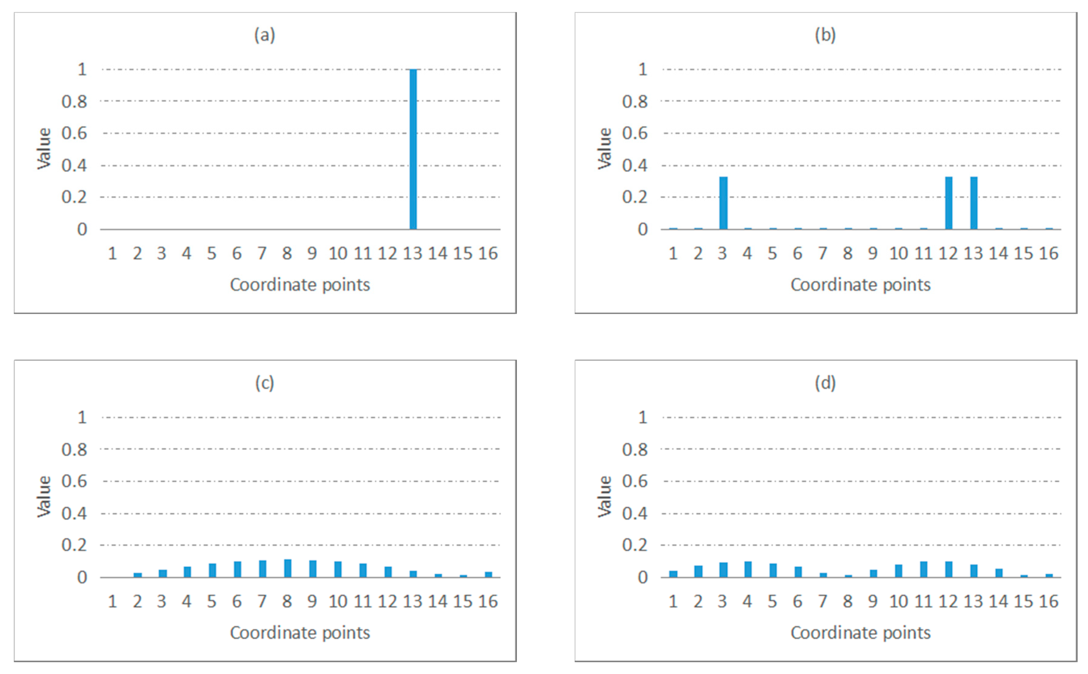
In the context of this paper, Shannon entropy is used to detect contrast or difference rather than probability. In a normalized set of data, Equation (1) assigns high values to functions where some values are much greater than others and low values to functions where all values are similar. This is illustrated in Figure 1 which shows four functions of 16 values, for each of which the values sum to unity. The function of Figure 1a has a unit value at one point and zero at all other points, i.e., one sharp peak. In the context of axle detection, this is the ideal situation and a wavelet scale giving this function would be favored. It has greatest contrast and the minimum possible entropy value of zero. The function of Figure 1b has three values of 0.33. This reduces the contrast and increases the entropy to 1.59. Figure 1c,d are sine wave functions with different frequency. The contrast is the same in both cases and significantly less than the other functions. The entropy value for both cases is 3.68. This figure shows that greater contrast functions result in lower values of Shannon entropy, making it a good indicator of contrast. For optimum axle identification from a series of wavelet results, the desired result is great contrast between the ‘axle part’ and the rest. Therefore, Shannon entropy is used here to guide the selection of optimum-contrast scale in the wavelet transform.
3. Wavelet Theory
The idea behind a wavelet analysis [37] is to express or to approximate the signal as a family of functions constructed from dilatations and translations of a single function called the base wavelet. Mathematically, the continuous wavelet transform of a function f(t) is defined as the integral transform of f(t) with a family of wavelet functions, ψa,b(t):
The function ψ (t) is generally called the base wavelet and the series of functions ψa,b(t) are called daughter wavelets. The daughter wavelets result from shifting and scaling the base wavelet. The scale factor, a, controls the scaling of the function ψ(t), and is inversely related to its frequency. The shift factor, b, controls the temporal translation of the function or its ‘location’ in the signal. In practice, wavelet functions can be dilated into infinitely large or infinitesimally small scales (a). A question that naturally arises is when or how to exit from the process of wavelet transformation; more specifically, what are the most relevant wavelet scales for a particular application?
Using the concept of Shannon entropy, this paper proposes to guide the selection of wavelet scale automatically by selecting the scale that gives greatest contrast or minimum entropy. The energy of the wavelet coefficients at scale a and location b is given by:
and the total energy of the function at scale, a is:
where N is the total number of wavelet coefficients. Then the entropy of the energy function is described using the concept of Shannon entropy as:
where is defined here as the relative wavelet energy at point, b:
Ref. [38] point out that the entropy function, is bounded by .
A lower Shannon entropy value corresponds to greater contrast and a higher energy concentration of the signals [36]. Therefore, an appropriate scale, corresponding to minimum Shannon entropy, should yield greater contrast in wavelet energy levels. For the purpose of detecting peaks caused by axles from strain signals in either SHM or BWIM systems, minimum Shannon entropy can guide the selection of the optimum scale of the wavelet transform, identifying the position of the discontinuities caused by the passing axles.
4. Numerical Simulation
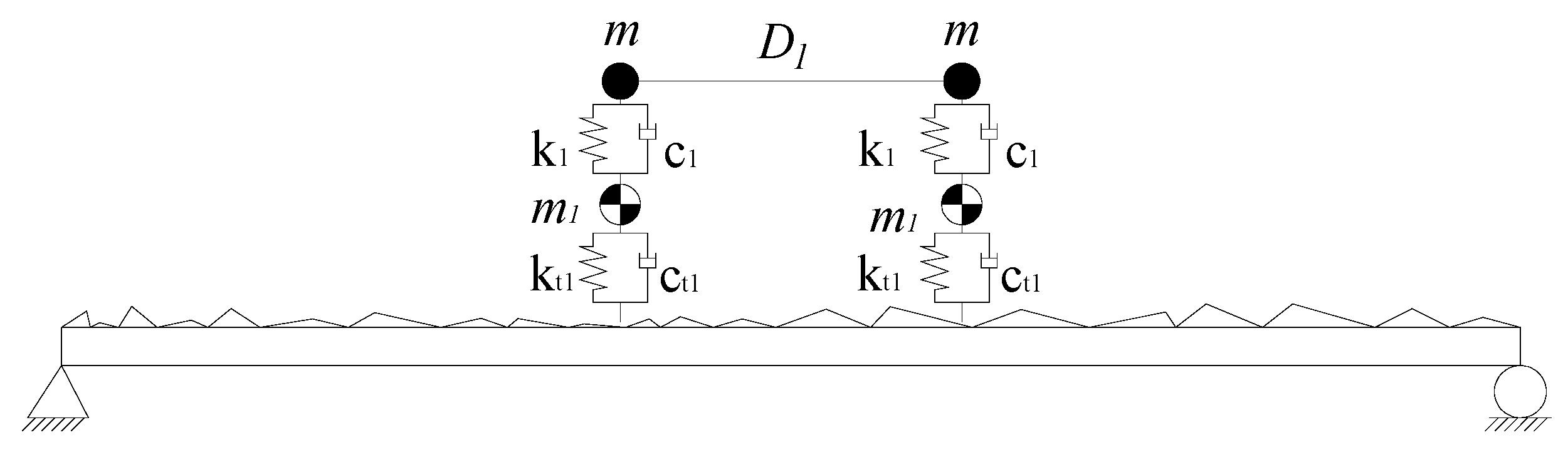
First, the vehicle is modeled crossing a 20 m approach distance followed by a 15 m simply supported bridge, as shown in Figure 2. The vehicle consists of two identical quarter-cars of equal sprung mass, m, and unsprung mass, m1. As the vehicle consists of independent quarter-cars, the pitching effect [39] is not explicitly considered in the simulation. The properties of the vehicle and bridge are listed in Table 1, which are intended to be realistic and are selected based on the references of [28,40,41]. Road surface roughness is considered in the form of a randomly generated profile of Class A, in accordance with ISO 8608 [42]. The scanning frequency is 500Hz.
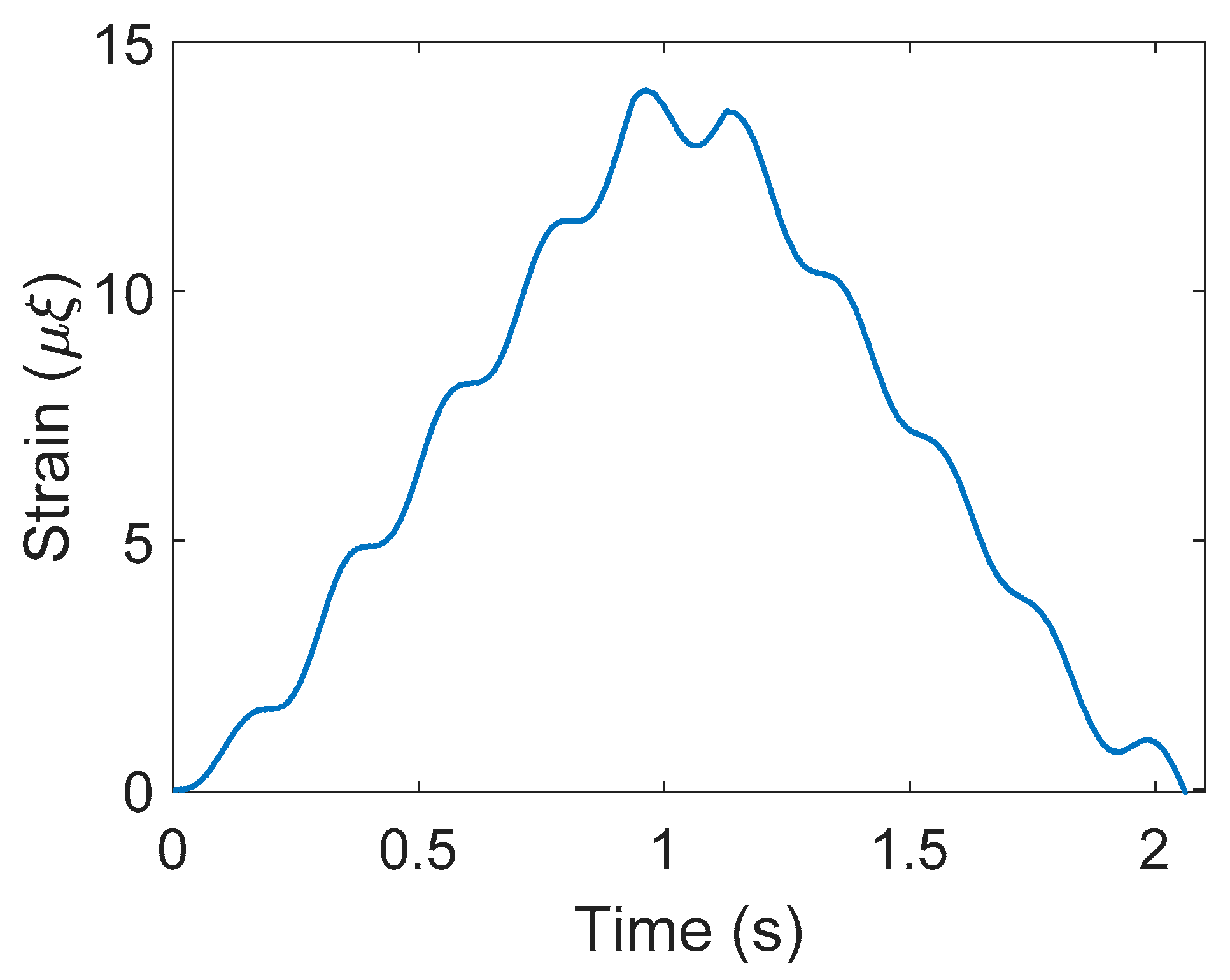
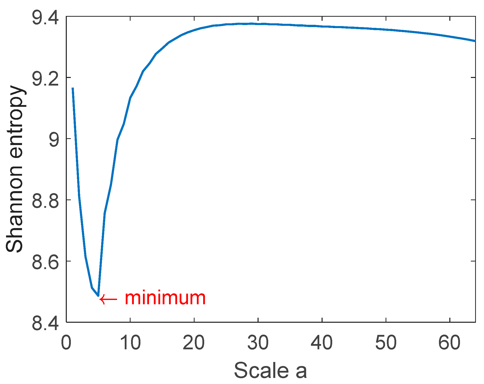
Figure 3 presents the calculated strain at mid-span when the vehicle passes over the bridge at a constant speed of 8 m/s. In practice, the FAD sensors are installed underneath the bridge slab, modeled here as a beam. It is not clear from the figure when either axle passes mid-span (times 0.94 and 1.13 s). A wavelet transform is used to further process this strain signal. At first, the signal is subject to a wavelet transform with a ‘db2’ Base wavelet and scales from 1 to 64, in unit increments. To find the optimal scale using the proposed Shannon entropy concept, the energy of the wavelet coefficients at each scale from 1 to 64 are calculated using Equation (4). Then, the relative wavelet energy at each scale is obtained by applying Equation (6). Finally, the wavelet entropy at each scale is computed with Equation (5) and the results presented in Figure 4. As shown, the minimum entropy occurs at a scale, a = 5, corresponding to a pseudo-frequency is 66.7 Hz.
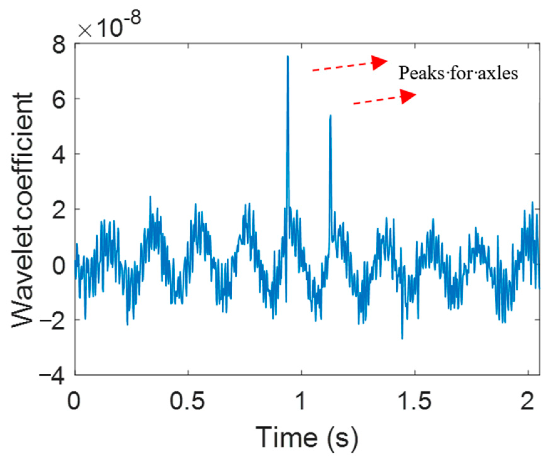
The wavelet function at this optimum scale is illustrated in Figure 5. Two peak values are clearly visible, indicating the times when the axles pass mid-span. This suggests that Shannon entropy can successfully identify a suitable scale for axle identification. Since the effect of road roughness is considered in the simulation, no clear peaks are evident in the mid-span strain signals as the axles arrive/leave the bridge.
5. The Selection of Mother Wavelet
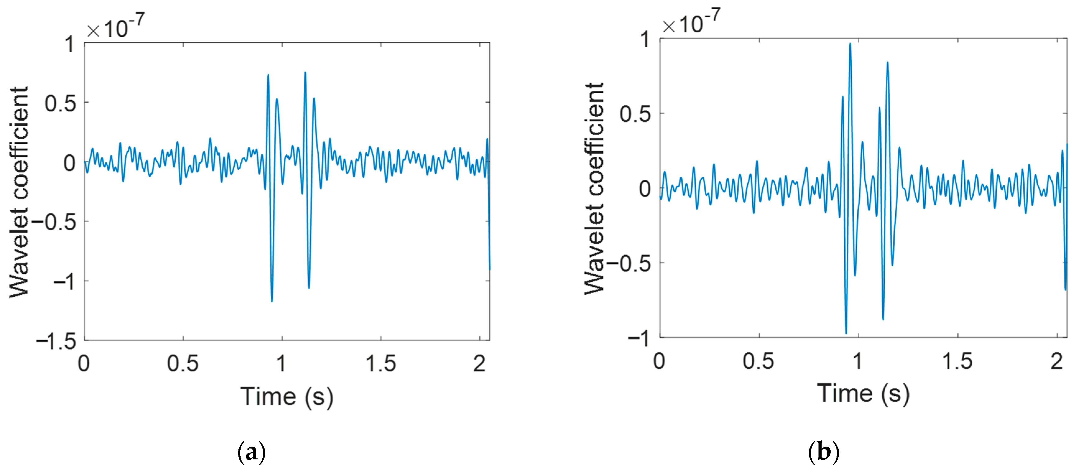
The above results were found using the Daubechies mother wavelet function, ‘db2’. Two other mother wavelet functions are tested here, db5 and db8, using the same signal as before (Figure 3). The results are illustrated in Figure 6, where it can be seen that there are now multiple closely spaced peaks corresponding to the passage of each axle. Since different mother wavelet functions generate different wavelet coefficients with different local patterns of peaks, a correlation coefficient is proposed to identify the mother wavelet function that most closely matches the original signal.
A correlation factor between the original signal and its wavelet coefficient is presented as:
where x is the original signal, y is the wavelet coefficient at the optimum scale and , are their respective mean values.
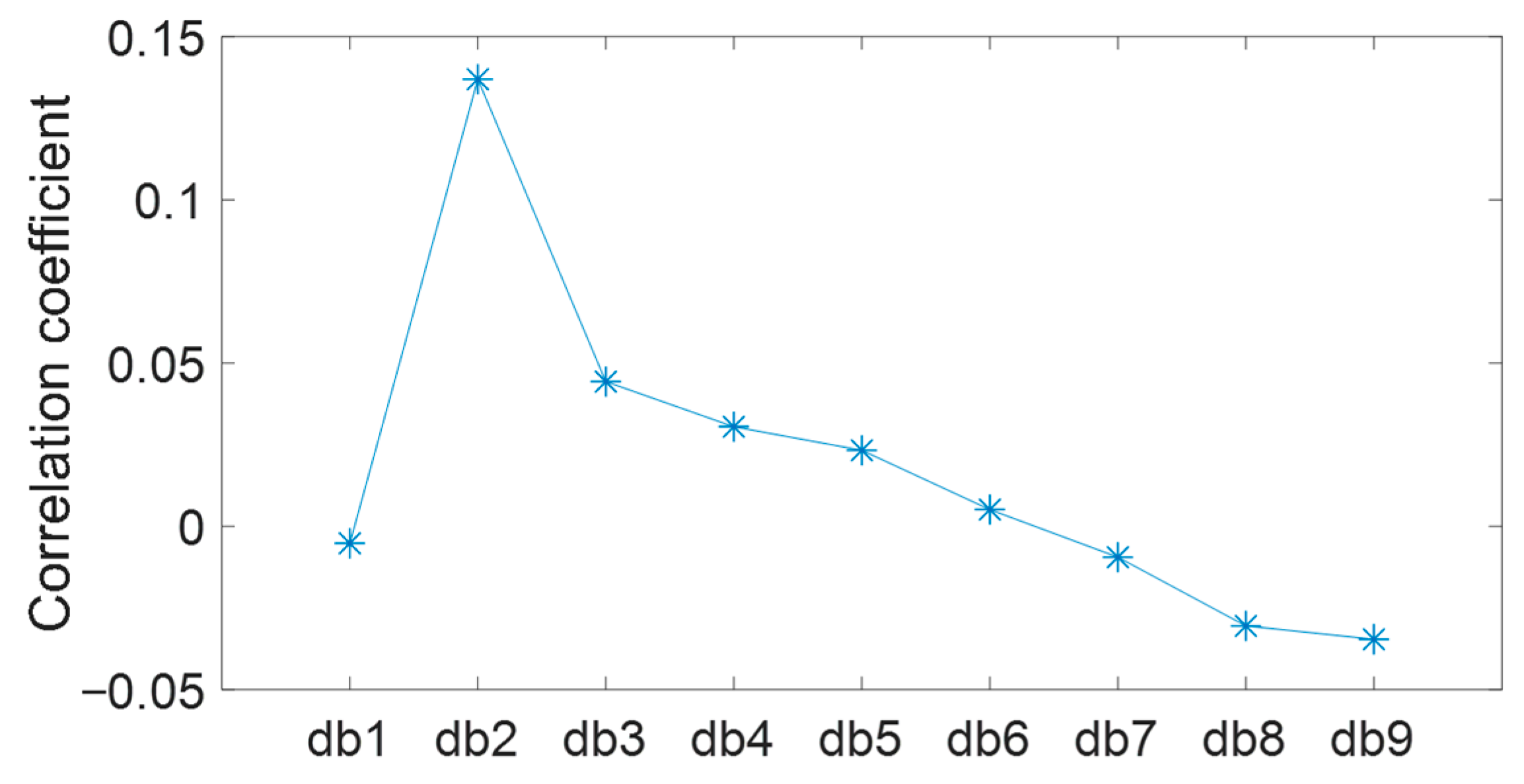
Considering the Daubechies wavelet family, the correlation coefficients are calculated for nine mother wavelets, each at its optimum scale, and illustrated in Figure 7. It can be seen that the ‘db2′ function has the maximum correlation coefficient.
6. Field Test of Fifth Wushui Bridge, China
6.1. Introduction to Field Test
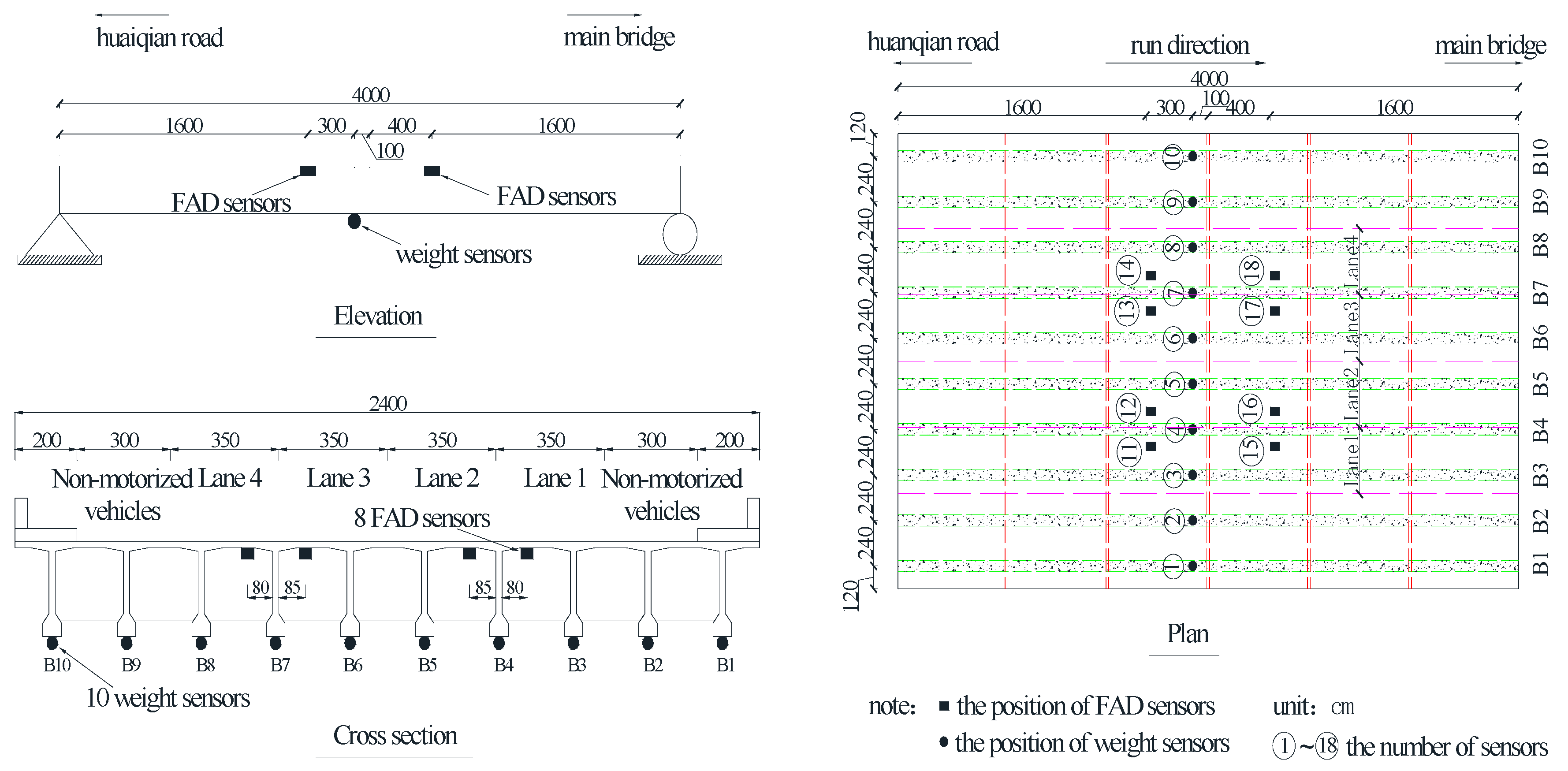
Field tests were conducted on an approach span of the Fifth Wushui Bridge, located in Huaihua, Hunan province, China. The test span is a simply supported 40 m long bridge constructed from ten parallel T-girders and carries four lanes of traffic—Figure 8. The main strain sensors used for inferring vehicle weights, numbered 1 to 10 in the figure, are located at mid-span on the soffits of Girder Nos. B1 to B10. Strain sensor Nos. 11 to 18 are used to detect the presence, location and speed of the axles in each lane, a key requirement of a BWIM system. The latter are known as free-of-axle-detector (FAD) sensors as they replace the road surface sensors used in early BWIM systems. This test uses the KD4001 strain sensor manufactured by Yangzhoukedong Co., Ltd., Jiangsu, China. The sensor uses a full-bridge circuit consisting of an electrical resistance foil strain gauge, which is connected to a heat-treated metal material to measure strain. This type of sensor can work in a harsh environment with temperature from −20° to 80°, but with a low level of sensitivity of 1.5 μξ. The measurement range is 0~1000 μξ and the bridge resistance is 350 Ω. All sensors are connected to a DC-204R collector, manufactured by Tokyo Sokki Kenkyujo Co., Ltd., Tokyo, Japan. The scanning frequency was 200 Hz. In the field test, two 2-axle rigid trucks, labelled A and B, passed the instrumented bridge repeatedly in each lane. Their characteristics are listed in Table 2.
6.2. Wavelet Analysis of Test Results for Single Truck Crossing
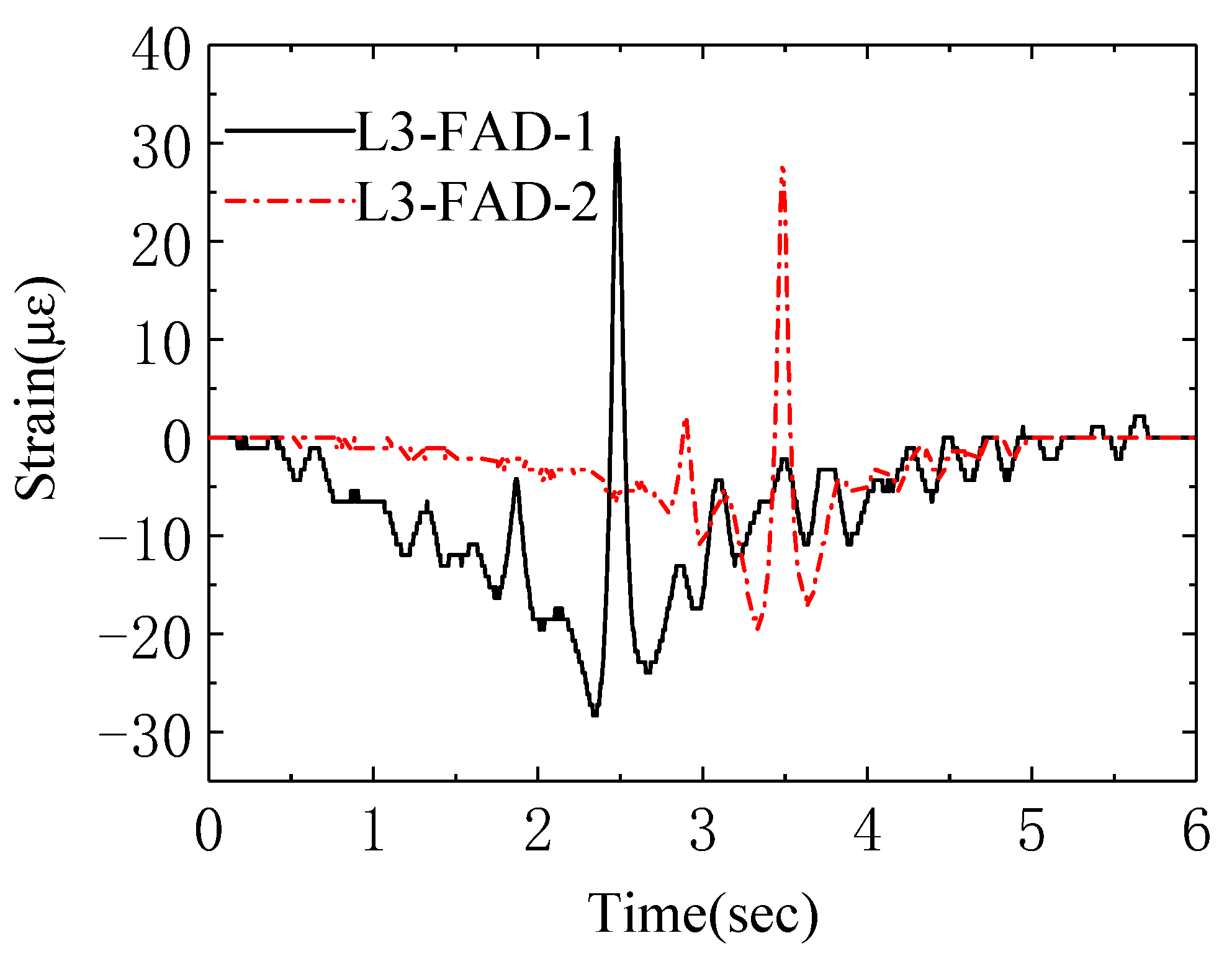
When an axle arrives or passes mid-span, the weighing sensors attached to the soffits of the girders exhibit a discontinuity of slope. The FAD sensors, because they are attached to the slab, have a much more ‘peaked’ response, ideally showing a significant peak when an axle passes. However, the peak is highly dependent on the transverse position of the wheel in the lane and whether it is over the girder web or the slab. If the vehicle deviates from the center line of the lane, the FAD sensors may not show clear peaks in response to passing axles [28]. For example, Figure 9 gives the (unprocessed) response to Truck A crossing the bridge in Lane 3, at Sensor 13 (labeled here as L3-FAD-1) and Sensor 17 (labeled as L3-FAD-2). It is noted that there was no filtering during data acquisition. Each FAD signal should have two peaks corresponding to the times when the two axles passed each sensor. However, there is only one obvious peak in each case. This could be because one of the axles had double tires and the other did not. Lesser peaks, before and after the dominant one, can be seen, but it is not clear which peaks correspond to passing axles and which are caused by vibration in the slab.
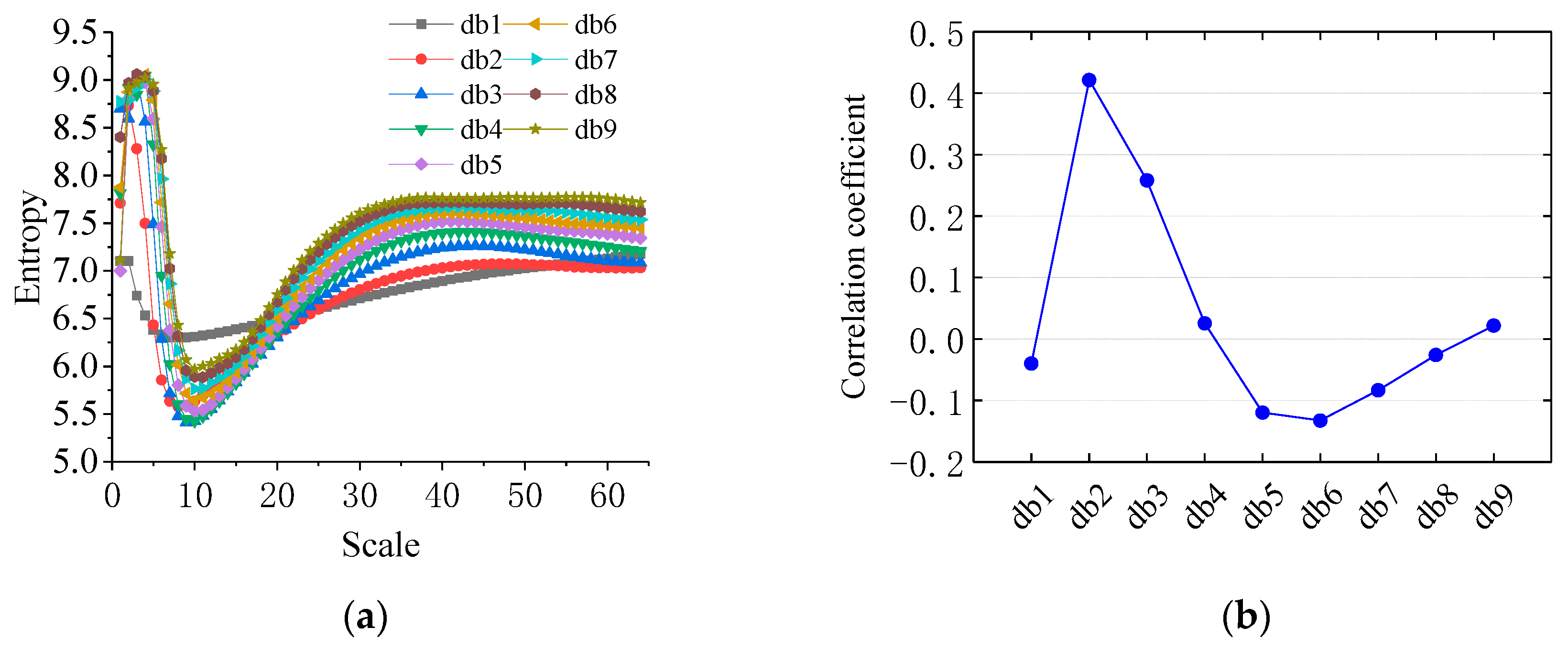
To improve axle detection, the L3-FAD-1 signal of Figure 9 is subjected to the proposed approach associated with the Daubechies wavelet family (db1-db9). All the computation is analyzed using the Matlab software, Version 2018b. The processor (CPU) is AMD Ryzen7 3700x 8-Core with 16 GB RAM. The operating system is Win 10. In this case, the computation time including calculation of wavelet transform, Shannon entropy, and correlation factor is 0.132s So far, the proposed method was not embedded in the BWIM system. But the computation time associated with all wavelet analysis is short, so the proposed method has the potential to be implemented in BWIM system for real-time application. As shown in Figure 10, the maximum correlation coefficient is again achieved with db2 for which the minimum Shannon entropy is at a scale of 8. The wavelet coefficients for this optimum mother wavelet and scale are plotted in Figure 11a. Two peaks are now clearly visible although the second is less pronounced than the first. Alternative transforms are illustrated in Figure 11 and show the effects of adopting sub-optimal scales (Figure 11b,c) and mother wavelets (Figure 11d–f). For example, the mother wavelet, db1 is anti-symmetric which makes it particularly difficult to detect the second peak. In summary, it is demonstrated that the wavelet transform, with Shannon entropy and correlation, can improve the ability of a FAD BWIM system to identify the presence of axles in FAD sensor signals.
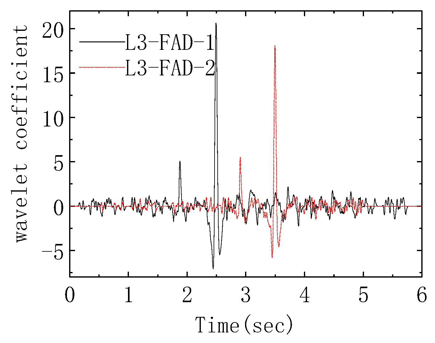
The same approach is applied to the L3-FAD-2 signal in Figure 9. The same mother wavelet, db2, and scale of 8 are found to be optimal for this signal. Figure 12 shows the transformed signals for both sensors. Unlike the raw signal of Figure 9, there are no other significant peaks that could be easily mistaken for axles.
The time stamps for the L3-FAD-1 signal peaks are 1.880 s and 2.490 s for the first and second peaks respectively. The corresponding respective time stamps for L3-FAD-2 are 2.905 s and 3.495 s. The interval between the main peaks in the two signals, with the known 8 m spacing between the sensors, provides the vehicle speed. This, with the 1st to 2nd peak (within-signal) intervals, is used to determine the axle spacing. The result is inferred spacings of 4.80 and 4.60 m from signals L3-FAD-1 and L3-FAD-2 respectively, just 2.1% above and below the statically measured spacing of 4.7 m. As shown, the identified axle spacing, which affects the axle weight recognition accuracy, is calculated based on the vehicle speed. Therefore, the vehicle speed is crucial for the BWIM system. In addition, there are additional 9 runs of single truck (No. A) passing over the test bridge on Lane 3. Similarly, their axle identifications are improved using the proposed wavelet-approach. The axle spacing based on the wavelet coefficient is calculated, in which the maximum errors from signals L3-FAD-1 and L3-FAD-2 are 5.3% and 5.7%, respectively. For all 10 runs, the mean and standard deviation of the errors are 1.5% and 2.7% for signals L3-FAD-1 respectively, and those for signals L3-FAD-2 are 0.9% and 2.9%, respectively.
6.3. Wavelet Analysis of Test Results with Multiple Presence
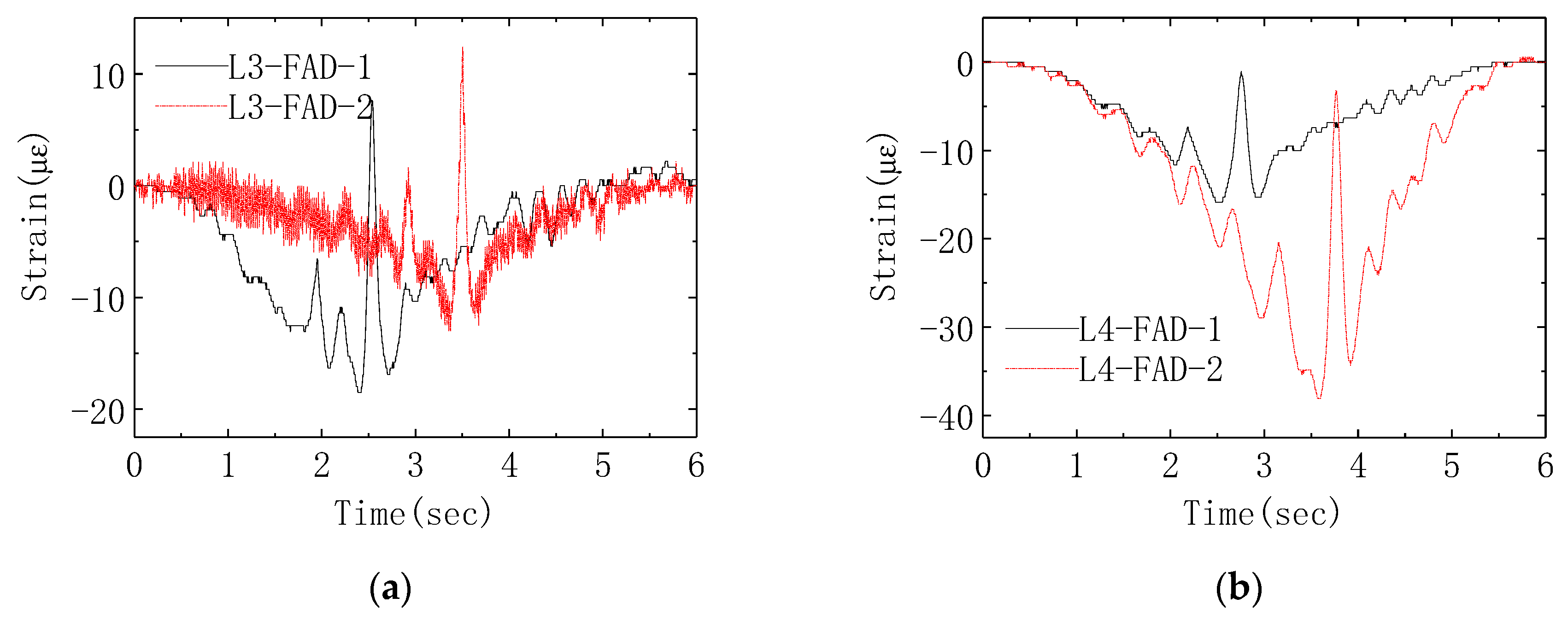
Axle detection is particularly challenging when there are multiple vehicles present, and this is especially the case when vehicles are present simultaneously in adjacent lanes. In one such run, the two trucks crossed the bridge simultaneously with Truck B in Lane 3 and Truck A in Lane 4. Like Lane 3, there are two FAD sensors in Lane 4, sensor numbers 14 (labeled L4-FAD-1) and 18 (labeled L4-FAD-2). All four raw FAD signals are illustrated in Figure 13. The signal for L3-FAD-2 is contaminated with significant white noise for reasons that are unclear.
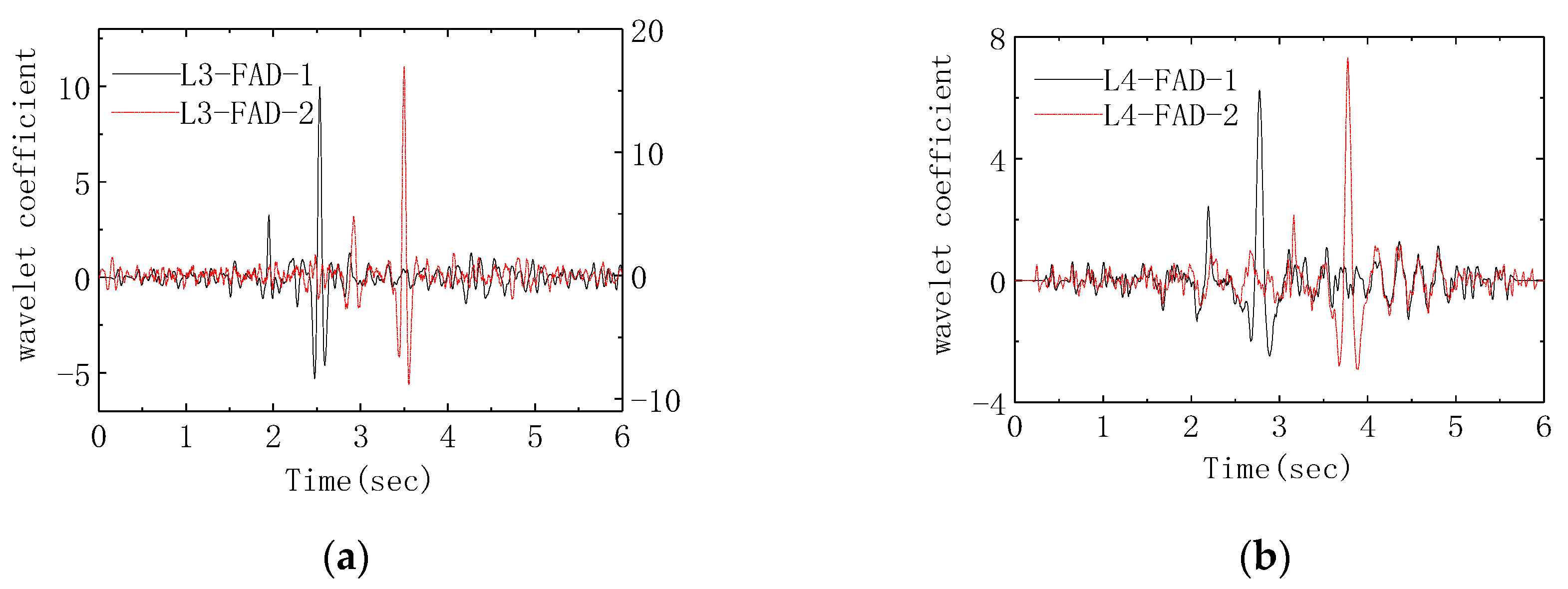
Each of these signals should have peaks corresponding to the two axles of the within-lane vehicle, with much lesser (and unwanted) peaks corresponding to the adjacent-lane vehicle. For both Lane 4 signals, there is one dominant peak with a secondary peak that may correspond to an axle or to general bridge vibration. Figure 14 shows the optimum results of the wavelet transform, where two peaks are now clearly visible in each signal. For this multiple-presence example, the inferred axle spacings are 4.71 m and 4.95 m for Truck A (Lane 4), which is 0.2% and 5.4% greater than the statically measured spacing of 4.7 m. It seems likely that the bridge vibration has combined with the second L4-FAD-2 peak, pushing its location to the left. The corresponding results for Truck B (Lane 3) are 4.80 m and 4.72 m (2.1% and 0.4% errors respectively). The noise in the original signal does not appear to have had an adverse influence on the accuracy.
7. Field Test on a Simply Supported Stiff Concrete Bridge
7.1. Test Bridge and Instrumentation
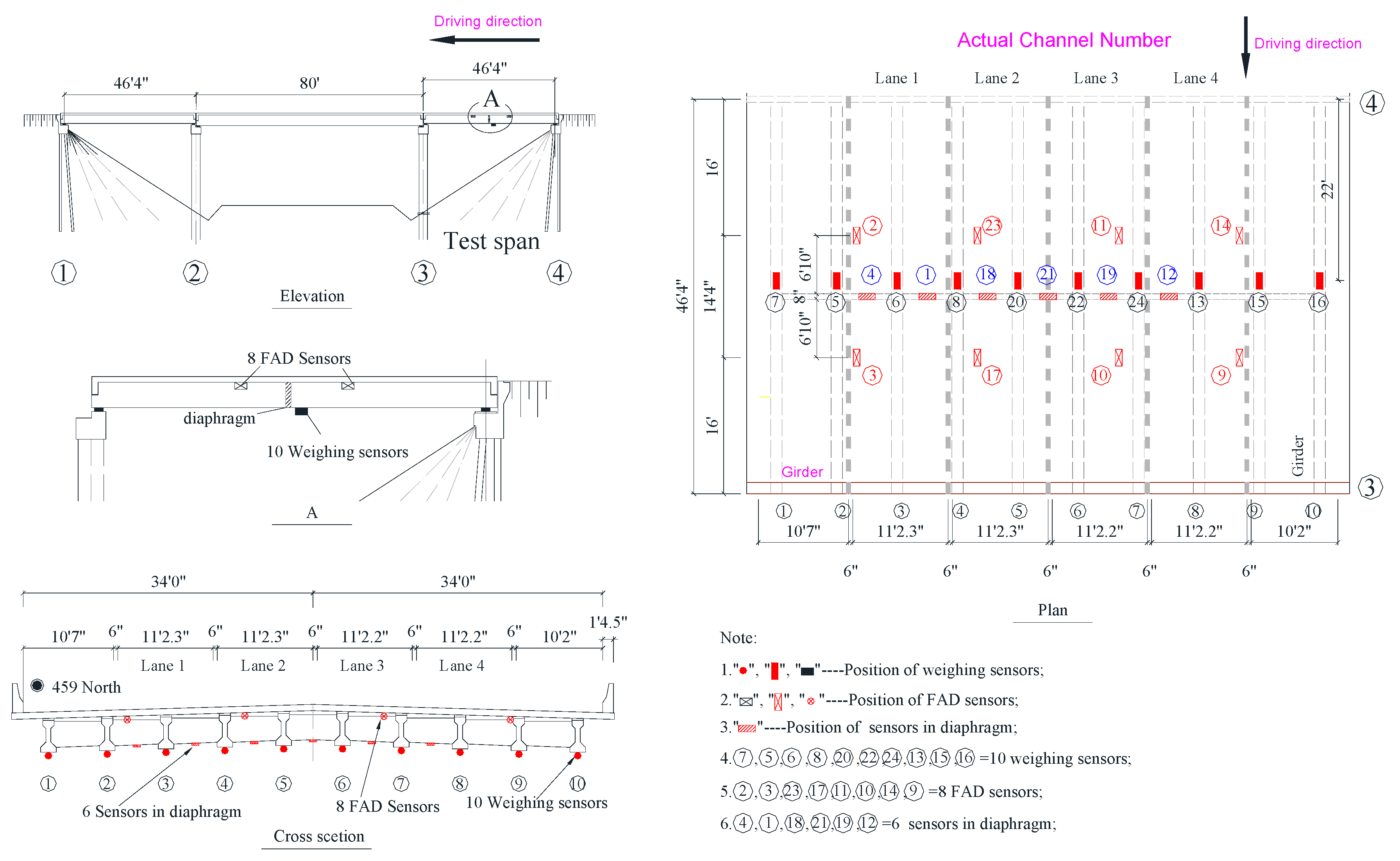
The second bridge selected for axle detection testing is located on Route 459 near Exit 10, about 25 km southwest of Birmingham, Alabama. The beam-and-slab bridge, identified as BIN No. 012296, was built in 1980 and is typical of highway bridges in Alabama and other American states. It consists of three simply supported spans of length, 14.04 m (46′4″), 24.38 m (80′) and 14.04 m (46′4″) with four same-direction lanes (Figure 15). The bridge has no skew angle with the abutments or piers.
The 14.04 m end span (3)–(4) was selected for testing. The bridge deck is 21.56 m (70′9″) wide and has ten pre-stressed concrete girders, as shown. Strain transducer weighing sensors were mounted longitudinally on the soffit of each concrete girder at mid-span. Eight FAD sensors, also strain transducers, were mounted longitudinally, 4.379 m (14′4″) apart, on the underside of the concrete slab. An additional six sensors (labeled here as Dia sensors) were mounted transversely on the internal diaphragm between adjacent girders from No. 2 to No. 8. In addition, a camera was installed on the site to monitor traffic in the relevant lanes. A commercial BWIM system (SiWIM) including sensors, data acquisition system, GMS connector, processor, etc., was used for the field test, where the ST350 strain transducers were used to measure the strains. The ST350 uses Wheatstone bridge circuitry with 350 Ω, which converts small changes in resistance to an output voltage that the data loggers can measure. Therefore, the recorded data is represented as a voltage signal, directly proportional to the strain signal. The sampling frequency was 500 Hz.
In the initial calibration testing, four calibration vehicles, one half-loaded and one full-loaded 3-axle rigid truck, and one half-loaded and one full-loaded 5-axle semi-trailer, ran repeatedly over the bridge, at different speeds and in different lanes. The details of the calibration vehicles are given in Table 3. The initial calibration procedure took two days without interrupting the traffic. During the calibration test, four calibration trucks passed over the bridge along different lanes 128 times (each calibration vehicle 32 runs).
7.2. Improved Axle Detection for Multiple Presence Loading Events
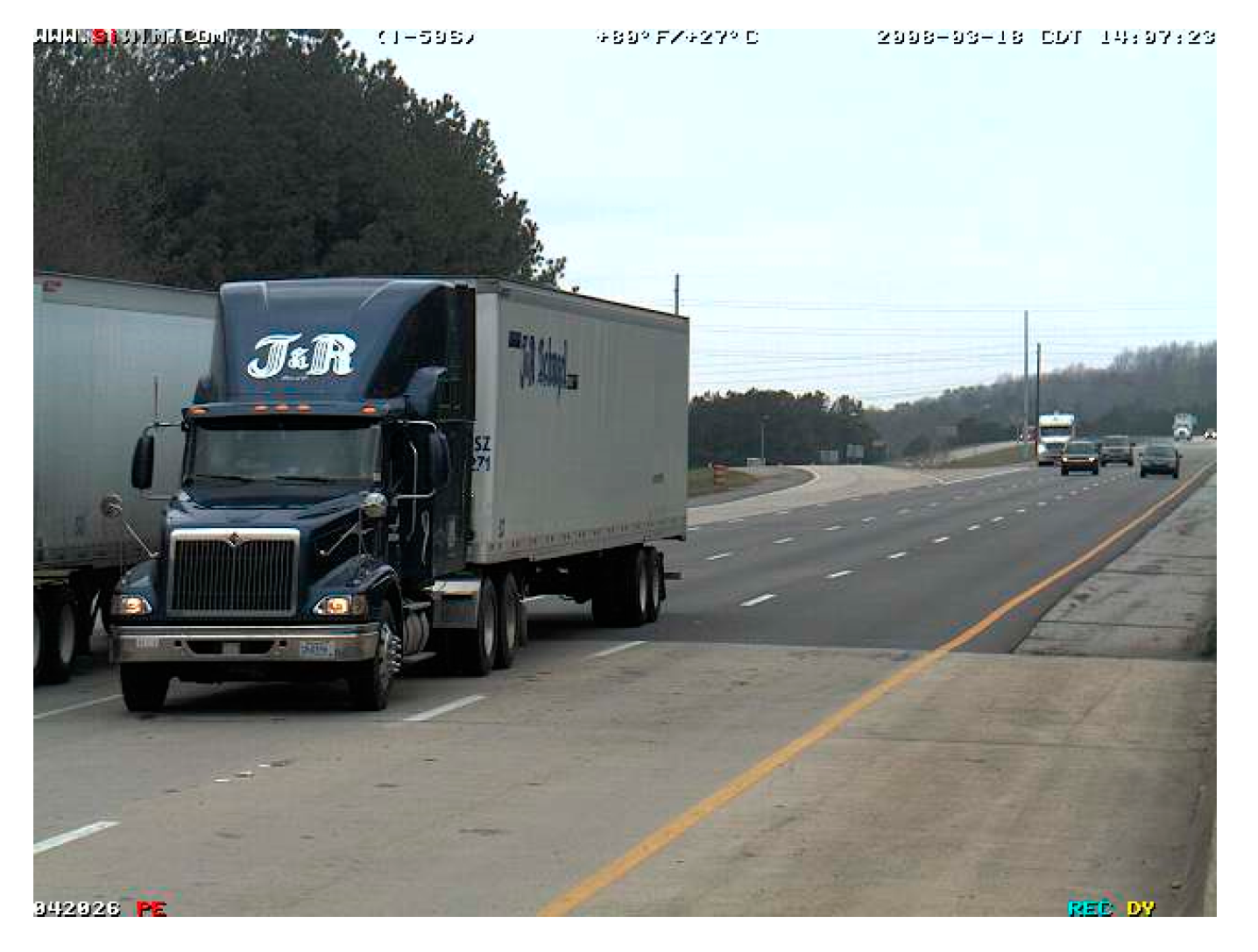
Figure 16 shows a multiple presence loading event on the bridge in traffic flow captured by the BWIM system. A truck is clearly visible in Lane 3, with a second truck to its left in Lane 2. The corresponding FAD signals are illustrated in Figure 17a. The raw Lane 2 signals, L2-FAD-1 and L2-FAD-2, show five peaks suggesting the presence of a 5-axle vehicle in that lane. Further, the spacing of these peaks suggest a vehicle of Class 9 according to the Federal Highways Administration classification system, i.e., a steer axle followed by two tandems. However, there is considerable vibration evident in the raw Lane 3 signals and a probable contribution of strain from the adjacent Lane 2 truck. As a result, the peaks corresponding to the second Class 9 truck are present but not clearly identifiable. Figure 17b shows that, after applying Shannon entropy and the correlation process, the Lane 3 wavelet coefficients provide clear peaks corresponding to each of the five axles. However, it is found that there are two small peaks caused by the bridge vibration between tandem wheels in L3-FAD-2, similar to the peak caused by the first axle, which may interfere with axle identification. Therefore, factors such as bridge vibration, multiple presence, low signal-to-noise ratio and even vehicle deviation within its lane, may negatively impact on the system’s ability to identify the passing axles. However, the proposed wavelet-based approach has shown robustness in terms of measurement noise in in the example of Figure 13.
Table 4 presents axle spacing errors for a sample of ten calibration vehicle and lane combinations. It should be noted that the greatest percentage errors (7.0% and 7.2%) are in the rear tandem of the 5-axle vehicle where the actual spacing is small (1.32 m). The mean and standard deviation of errors in (A2–A3) are 1.45% and 4% respectively, and those for (A4–A5) are 5.24% and 2.6%, respectively. For the larger spacings, there remain some significant errors—see, for example, an error of 5.1% in Run 10. The mean and standard deviation of errors in (A1–A2) are 1.79% and 1.26% respectively, and those for (A3–A4) are 0.18% and 0.47% respectively.
8. Conclusions
For beam-and-slab bridges, FAD sensors mounted under the slab are used to determine the vehicle configuration (vehicle speed, axle number, and axle spacing), which is required information for BWIM systems and some aspects of SHM systems. However, field tests have shown that FAD signals sometimes fail to clearly identify vehicle axles. This can be due to bridge vibration, multiple vehicle presence, or deviation of vehicles transversely in their lane. This paper proposes a wavelet-based approach, with Shannon entropy and a correlation factor, to enhance axle detection from FAD signals. The mother wavelet with maximum correlation, combined with the scale of least Shannon entropy, is used to automatically select an optimum transform. The fidelity of the proposed approach is investigated including measurement noise, multiple presence, different vehicle velocities, different types of vehicle and even in real traffic flow conditions. In this paper, only heavy trucks are used in the two field tests. Investigating the feasibility of axle identification for lightweight vehicles using the proposed algorithm is planned as future work.
Author Contributions
Conceptualization, C.T. and H.Z.; methodology, C.T.; software, C.T.; validation, E.J.O., N.U. and B.Z.; formal analysis, C.T.; investigation, N.U.; resources, H.Z.; data curation, B.Z.; writing—original draft preparation, C.T.; writing—review and editing, E.J.O.; visualization, C.T.; supervision, H.Z. and E.J.O.; project administration, C.T. and H.Z.; funding acquisition, C.T. and H.Z. Please turn to the CRediT taxonomy for the term explanation. Authorship must be limited to those who have contributed substantially to the work reported. All authors have read and agreed to the published version of the manuscript.
Funding
This research was funded by National Natural Science Foundation of China (No. 52008162) and the Key Research and Development Program of Hunan Province (No. 2019SK2172).
Conflicts of Interest
The authors declare no conflict of interest.
References
- ASCE. 2017 Infrastructure Report Card; Technical Report; ASCE: Reston, VA, USA, 2017. [Google Scholar]
- Yau, J.D.; Yang, J.P.; Yang, Y.B. Wave number-based technique for detecting slope discontinuity in simple beams using moving test vehicle. Int. J. Struct. Stab. Dyn. 2017, 17, 1750060. [Google Scholar] [CrossRef]
- Cantero, D.; González, A. Bridge Damage Detection Using Weigh-in-Motion Technology. J. Bridge Eng. 2015, 20, 04014078. [Google Scholar] [CrossRef] [Green Version]
- Ono, R.; Ha, T.M.; Fukada, S. Analytical study on damage detection method using displacement influence lines of road bridge slab. J. Civ. Struct. Health Monit. 2019, 9, 565–577. [Google Scholar] [CrossRef]
- Hester, D.; Brownjohn, J.; Huseynov, F.; OBrien, E.; Gonzalez, A.; Casero, M. Identifying damage in a bridge by analysing rotation response to a moving load. Struct. Infrastruct. Eng. 2020, 16, 1050–1065. [Google Scholar] [CrossRef]
- Yang, Y.B.; Yang, J.P. State-of-the-art review on modal identification and damage detection of bridges by moving test vehicles. Int. J. Struct. Stab. Dyn. 2018, 18, 1850025. [Google Scholar] [CrossRef]
- Yang, Y.B.; Yang, J.P.; Zhang, B.; Wu, Y. Vehicle Scanning Method for Bridges; Wiley: Hoboken, NJ, USA, 2020. [Google Scholar]
- Gonzalez, A.; Dowling, J.; O’Brien, E.; Znidaric, A. Testing of a Bridge Weigh-in-Motion Algorithm Utilising Multiple Longitudinal Sensor Locations. J. Test. Eval. 2012, 40, 961–974. [Google Scholar] [CrossRef]
- Moses, F. Weigh-in-motion system using instrumented bridges. Transp. Eng. 1979, 3, 233–249. [Google Scholar]
- Moses, F.; Ghosn, M. Weighing Trucks-in-Motion Using Instrumented Highway Bridges: Final Report; Case Western University: Cleveland, OH, USA, 1981. [Google Scholar]
- OBrien, E.J.; Quilligan, M.J.; Karoumi, R. Calculating an influence line from direct measurements. In Proceedings of the Institution of Civil Engineers-Bridge Engineering; Thomas Telford Ltd.: London, UK, 2006; Volume 159, pp. 31–34. [Google Scholar]
- Yamaguchi, E.; Kawamura, S.-I.; Matuso, K.; Matsuki, Y.; Naito, Y. Bridge-Weigh-In-Motion by Two-Span Continuous Bridge with Skew and Heavy-Truck Flow in Fukuoka Area, Japan. Adv. Struct. Eng. 2009, 12, 115–125. [Google Scholar] [CrossRef]
- Lydon, M.; Robinson, D.; Taylor, S.E.; Amato, G.; OBrien, E.J.; Uddin, N. Improved axle detection for bridge weigh-in-motion systems using fiber optic sensors. J. Civ. Struct. Health Monit. 2017, 7, 325–332. [Google Scholar] [CrossRef] [Green Version]
- Chen, S.Z.; Wu, G.; Feng, D.C. Development of a bridge weigh-in-motion method considering the presence of multiple vehicles. Eng. Struct. 2019, 191, 724–739. [Google Scholar] [CrossRef]
- Oskoui, E.A.; Taylor, T.; Ansari, F. Method and sensor for monitoring weight of trucks in motion based on bridge girder end rotations. Struct. Infrastruct. Eng. 2020, 16, 481–494. [Google Scholar] [CrossRef]
- Alamandala, S.; Prasad, R.S.; Kumar, P.R.; Kumar, M.R. Damage Detection in Bridge-Weigh-In-Motion Structures using Fiber Bragg Grating Sensors. In Laser Science (pp. JW3A-103); Optical Society of America: Washington, DC, USA, 2018. [Google Scholar]
- Moses, F. Instrumentation for Weighing Trucks-in-Motion for Highway Bridge Loads; Final Report; National Technical Information Service: Springfield, WV, USA, 1983.
- Znidaric, A.; Dempsey, A.; Lavric, I.; Baumgaertner, W. Bridge WIM Systems without Axle Detectors; Hermes Science: Paris, France, 1999; pp. 101–110. [Google Scholar]
- Znidaric, A.; Lavric, I.; Kalin, J. Bridge WIM Measurements on Short Slab Bridges; Hermes Science: Paris, France, 1999; pp. 217–225. [Google Scholar]
- Zhang, L. An Evaluation of the Technical and Economic Performance of Weigh-In-Motion Sensing Technology. Master’s Thesis, University of Waterloo, Waterloo, ON, Canada, 2007. [Google Scholar]
- Kalin, J.; Žnidarič, A.; Lavrič, I. Practical implementation of nothing-on-the-road bridge weigh-in-motion system. In International Symposium on Heavy Vehicle Weights and Dimensions. 2006. Available online: https://hvttforum.org/wp-content/uploads/2019/11/Practical-Implementation-of-Nothing-on-the-Road-Bridge-Weigh-In-Motion-System-Kalin.pdf (accessed on 27 September 2020).
- Peters, R.J. Axway-A system to obtain vehicle axle weights. Victoria. In Australian Road Research; Australian Road Research Board (ARRB): Victoria, Australia, 1984; Volume 12, pp. 10–18. [Google Scholar]
- Peters, R.J. Culway-An unmanned and undetectable highway speed vehicle weighing system. In Australian Road Research; Australian Road Research Board (ARRB): Victoria, Australia, 1986; Volume 13, pp. 70–83. [Google Scholar]
- Brown, A.J. Bridge Weigh-in-Motion Deployment Opportunities in Alabama; Jones, S., Richardson, J., Lindly, J., Weber, J., Eds.; ProQuest Dissertations Publishing: Ann Arbor, MI, USA, 2011. [Google Scholar]
- Kalhori, H.; Makki Alamdari, M.; Zhu, X.; Samali, B. Nothing-on-Road Axle Detection Strategies in Bridge-Weigh-in-Motion for a Cable-Stayed Bridge: Case Study. J. Bridge Eng. 2018, 23, 05018006. [Google Scholar] [CrossRef]
- OBrien, E.J.; Zhang, L.; Zhao, H.; Hajializadeh, D. Probabilistic bridge weigh-in-motion. Can. J. Civ. Eng. 2018, 45, 667–675. [Google Scholar] [CrossRef] [Green Version]
- He, W.; Ling, T.; OBrien, E.J.; Deng, L. Virtual Axle Method for Bridge Weigh-in-Motion Systems Requiring No Axle Detector. J. Bridge Eng. 2019, 24, 04019086. [Google Scholar] [CrossRef]
- Chatterjee, P.; OBrien, E.; Li, Y.; Gonzáilez, A. Wavelet domain analysis for identification of vehicle axles from bridge measurements. Comput. Struct. 2006, 84, 1792–1801. [Google Scholar] [CrossRef] [Green Version]
- Hitchcock, W.A.; Uddin, N.; Sisiopiku, V.; Salama, T.; Kirby, J.; Zhao, M.H.; Toutanji, H.; Richardson, J. Bridge Weigh-in-Motion (B-WIM) System Testing and Evaluation; UTCA Project (07212); University Transportation Center for Alabama: Tuscaloosa, AL, USA, 2012. [Google Scholar]
- Dunne, D.; O’Brien, E.J.; Basu, B.; Gonzalez, A. Bridge WIM systems with Nothing on the Road (NOR). In Proceedings of the 4th International Conference on Weigh-In-Motion, Taipei, Taiwan, 20–23 February 2005; National Taiwan University: Taipei, Taiwan, 2005; p. 9. [Google Scholar]
- Yu, Y.; Cai, C.S.; Deng, L. Vehicle axle identification using wavelet analysis of bridge global responses. J. Vib. Control. 2017, 23, 2830–2840. [Google Scholar] [CrossRef]
- Blackburn, S. The Oxford Dictionary of Philosophy; OUP Oxford: Oxford, UK, 2005. [Google Scholar]
- Saviotti, P.P. Information, variety and entropy in technoeconomic development. Res. Policy 1988, 17, 89–103. [Google Scholar] [CrossRef]
- Shannon, C.E. A mathematical theory of communication. ACM Sigmobile Mobile Comput. Commun. Rev. 2001, 5, 3–55. [Google Scholar] [CrossRef]
- de Oliveira, H.M.; de Souza, D.F. Wavelet analysis as an information processing technique. In 2006 International Telecommunications Symposium; IEEE: New York, NY, USA, 2006. [Google Scholar]
- Bulusu, K.V.; Plesniak, M.W. Shannon entropy-based wavelet transform method for autonomous coherent structure identification in fluid flow field data. Entropy 2015, 17, 6617–6642. [Google Scholar] [CrossRef]
- Morlet, J.; Arens, G.; Fourgeau, E.; Glard, D. Wave propagation and sampling sampling theory; Part I: Complex signal and scattering in multilayered media. Geophysics 1982, 47, 203–221. [Google Scholar] [CrossRef] [Green Version]
- Cebon, D. Handbook of Vehicle-Road Interaction; CRC Press: Boca Raton, FL, USA, 1999. [Google Scholar]
- Yang, J.P.; Sun, J.Y. Pitching effect of a three-mass vehicle model for analyzing vehicle-bridge interaction. Eng. Struct. 2020, 224, 111248. [Google Scholar] [CrossRef]
- Gao, R.X.; Yan, R. Selection of Base Wavelet; Springer: Boston, MA, USA, 2011. [Google Scholar]
- Harris, N.K.; OBrien, E.J.; González, A. Reduction of bridge dynamic amplification through adjustment of vehicle suspension damping. J. Sound Vib. 2007, 302, 471–485. [Google Scholar] [CrossRef] [Green Version]
- ISO. Mechanical Vibration—Road Surface Profiles—Reporting of Measured Data; International Organization for Standardization: Geneva, Switzerland, 1995. [Google Scholar]
Figure 1.
Four different functions of 16 values. (a) one point has value of one; (b) three points have values of 0.33; (c) sine wave function; (d) sine wave function with different frequency.
Figure 1.
Four different functions of 16 values. (a) one point has value of one; (b) three points have values of 0.33; (c) sine wave function; (d) sine wave function with different frequency.

Figure 2.
Bridge and vehicle model.

Figure 3.
Calculated strain signal at bridge mid-span.

Figure 4.
Shannon entropy values for each scale.

Figure 5.
Wavelet coefficient at scale 5.

Figure 6.
Optimum axle identification using different Daubechies mother wavelet functions: (a) db5, scale = 11, (b) db8, scale = 13.
Figure 6.
Optimum axle identification using different Daubechies mother wavelet functions: (a) db5, scale = 11, (b) db8, scale = 13.

Figure 7.
Correlation coefficient for different mother wavelet functions.

Figure 8.
Wushui test bridge and sensor positions.

Figure 9.
The strain signal of free-of-axel-detector (FAD) sensors in Lane 3.

Figure 10.
Shannon entropy and correlation coefficient for L3-FAD-1 signal; (a) Shannon entropy; (b) correlation coefficient.
Figure 10.
Shannon entropy and correlation coefficient for L3-FAD-1 signal; (a) Shannon entropy; (b) correlation coefficient.

Figure 11.
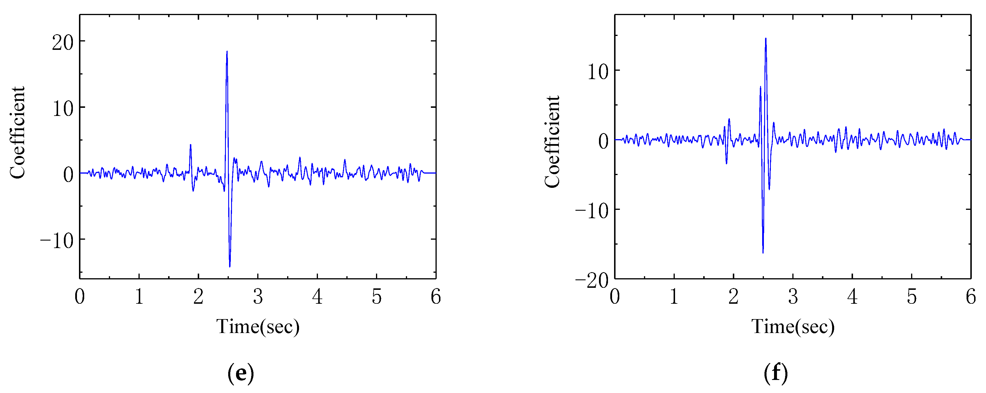
Wavelet coefficients for different mother wavelets and scales: (a) db2, scale = 8 (optimal); (b) db2, scale = 4 (less than optimal); (c) db2, scale = 16 (greater than optimal); (d) db1, scale = 7 (optimal); (e) db3, scale = 9 (optimal); (f) db6, scale = 10 (optimal).
Figure 11.
Wavelet coefficients for different mother wavelets and scales: (a) db2, scale = 8 (optimal); (b) db2, scale = 4 (less than optimal); (c) db2, scale = 16 (greater than optimal); (d) db1, scale = 7 (optimal); (e) db3, scale = 9 (optimal); (f) db6, scale = 10 (optimal).


Figure 12.
Wavelet coefficient functions for Lane 3 FAD signals (both with db2 at scale of 8).

Figure 13.
Raw FAD signals for multiple presence loading event: (a) Truck B in Lane 3; (b) Truck A in Lane 4.
Figure 13.
Raw FAD signals for multiple presence loading event: (a) Truck B in Lane 3; (b) Truck A in Lane 4.

Figure 14.
Wavelet coefficients for multiple-presence loading event: (a) Truck B in Lane 3; (b) Truck A in Lane 4.
Figure 14.
Wavelet coefficients for multiple-presence loading event: (a) Truck B in Lane 3; (b) Truck A in Lane 4.

Figure 15.
Geometry and sensor locations on Route 459 bridge (units: feet’ and inches”).

Figure 16.
Photograph of trucks in Lane 2 and Lane 3.

Figure 17.
Case study of multiple presence loading event: (a) raw signals; (b) optimal wavelet coefficients.
Figure 17.
Case study of multiple presence loading event: (a) raw signals; (b) optimal wavelet coefficients.


Table 1.
Properties of vehicle and bridge models.
| Vehicle Properties | Bridge Properties | ||
|---|---|---|---|
| D1 | 1.5 m | Span | 15 m |
| m | 5000 kg | Density | 4800 kg/m3 |
| k1 | 3500 kN/m | Second moment of area of cross-section | 0.365 m4 |
| c1 | 10 kN s/m | Modulus of elasticity | 3.5 × 10¹⁰ N/m2 |
| m1 | 750 kg | Damping ratio | 0.01 |
| kt1 | 350 kN/m | Breadth | 6 m |
| ct1 | 0 | Depth | 0.9 m |
Table 2.
Vehicle characteristics.
| Axle 1 | Axle 2 | ||
|---|---|---|---|
| Truck A | Axle spacing (m) | 4.7 | |
| Axle weight (tonnes) | 5.8 | 24.5 | |
| Truck B | Axle spacing (m) | 4.7 | |
| Axle weight (tonnes) | 7.4 | 21.1 | |
Table 3.
Calibration vehicle weights and spacings.
| Vehicle No. | Axle Weight (Kips) | Axle Spacing (Inches) | ||||||||
|---|---|---|---|---|---|---|---|---|---|---|
| GVW | 1st axle | 2nd axle | 3rd axle | 4th axle | 5th axle | A1-A2 | A2-A3 | A3-A4 | A4-A5 | |
| 1 | 80.1 | 21.5 | 29.7 | 28.9 | 223 | 56 | ||||
| 2 | 41.1 | 20.0 | 10.8 | 10.3 | 223 | 56 | ||||
| 3 | 79.8 | 10.5 | 15.4 | 16.4 | 18.6 | 18.9 | 172 | 52 | 438 | 52 |
| 4 | 41.1 | 10.7 | 7.8 | 7.7 | 7.4 | 7.5 | 172 | 52 | 438 | 52 |
Note: 1 kip = 453.59 kg, 1 inch = 25.4 mm; GVW: gross of vehicle weight; ith axle represents the weight of the ith axle; Ai-Ai+1 represents the distance between adjacent axes.
Table 4.
Vehicle speeds and errors in axle spacings.
| Item | Axle Spacing | Run 1 | Run 2 | Run 3 | Run 4 | Run 5 | Run 6 | Run 7 | Run 8 | Run 9 | Run 10 | Mean | SD |
|---|---|---|---|---|---|---|---|---|---|---|---|---|---|
| Truck no. | 3 | 3 | 3 | 3 | 4 | 2 | 2 | 2 | 1 | 1 | / | / | |
| Lane | 1 | 1 | 2 | 2 | 2 | 1 | 1 | 1 | 1 | 2 | / | / | |
| Speed (m/s) | 30.5 | 30.5 | 29.9 | 30.5 | 30.1 | 27.7 | 28.2 | 27.8 | 28.2 | 28.2 | |||
| Error in axle spacing (relative to static measurement) | A1-A2 | −0.50% | −1.10% | −1.00% | −1.80% | −0.30% | −3.80% | −3.70% | −3.10% | −2.00% | −0.60% | −1.79% | 1.26% |
| A2-A3 | 3.60% | 0% | −2.70% | −2.40% | −6.40% | 4.70% | 4.50% | 3.40% | 4.70% | 5.10% | 1.45% | 4.00% | |
| A3-A4 | −0.40% | −0.80% | −0.30% | 0% | 0.60% | / | / | / | / | / | −0.18% | 0.47% | |
| A4-A5 | −5.40% | −0.20% | −7.20% | −7.00% | −6.40% | / | / | / | / | / | −5.24% | 2.60% |
Note: “Ai–Aj” means spacing between axles i and j; SD represents the standard deviation.
Publisher’s Note: MDPI stays neutral with regard to jurisdictional claims in published maps and institutional affiliations. |
© 2020 by the authors. Licensee MDPI, Basel, Switzerland. This article is an open access article distributed under the terms and conditions of the Creative Commons Attribution (CC BY) license (http://creativecommons.org/licenses/by/4.0/).
Share and Cite
MDPI and ACS Style
Zhao, H.; Tan, C.; OBrien, E.J.; Uddin, N.; Zhang, B. Wavelet-Based Optimum Identification of Vehicle Axles Using Bridge Measurements. Appl. Sci. 2020, 10, 7485. https://doi.org/10.3390/app10217485
AMA Style
Zhao H, Tan C, OBrien EJ, Uddin N, Zhang B. Wavelet-Based Optimum Identification of Vehicle Axles Using Bridge Measurements. Applied Sciences. 2020; 10(21):7485. https://doi.org/10.3390/app10217485
Chicago/Turabian StyleZhao, Hua, Chengjun Tan, Eugene J. OBrien, Nasim Uddin, and Bin Zhang. 2020. "Wavelet-Based Optimum Identification of Vehicle Axles Using Bridge Measurements" Applied Sciences 10, no. 21: 7485. https://doi.org/10.3390/app10217485
Note that from the first issue of 2016, this journal uses article numbers instead of page numbers. See further details here.