Pressure Loss Optimization to Reduce Pipeline Clogging in Bulk Transfer System of Offshore Drilling Rig

Featured Application

The proposed improved bulk transfer system is expected to contribute toward reducing uncertainty and minimizing maintenance and repair costs during operation.

Abstract

In offshore drilling systems, the equipment localization rate is less than 20%, and the monopoly of a few foreign conglomerates over the equipment is intensifying. To break this monopoly, active technology development and market entry strategies are required. In a drillship or a floating production, storage, and offloading unit, the distance from the tank top to the upper deck is approximately 30–40 m. Therefore, the pressure loss problem inside the vertical pipe from the tank to the deck should be considered. To transport the bulk at the target transport rate without clogging, the pressure loss inside the vertical pipe should be optimized. Moreover, the operating pressure, air volume, and transport rate accuracy determine the system and operating costs. Hence, system optimization is necessary. In this study, pressure loss modeling and simulation of the bulk transfer system are performed to prevent frequent pipeline clogging. The proposed simulation model is verified using real test data. The bulk transfer system is verified through a simulation, indicating an error rate of 4.27%. In addition, the number of air boosters required to minimize the pipeline’s pressure loss and the optimal distance between the boosters are obtained using a genetic algorithm. With the optimized air booster, pressure loss for approximately 0.54 bar was compensated. The improved bulk transfer system is expected to reduce uncertainty and minimize maintenance and repair costs during operation. Moreover, it can contribute to high-value fields such as construction, commissioning, installation, maintenance, and equipment localization improvement.

1. Introduction

Offshore drilling is a mechanical process in which a wellbore is drilled into the seabed. In an offshore drilling system, a subsea well is drilled from a drilling rig using a subsea wellhead located below the rig, and a wellhead stack is mounted on the subsea wellhead [1]. Drilling in the ocean is largely classified into bottom supported rigs and floating rigs; it can be further classified into platform, jack-up, submersible, semi-submersible, and drillship. The mud circulation system is the modern solution to an environmentally sensitive drilling operation. The circulation system on the rig is fully self-supporting, requiring only the discharge of drill cuttings [2].

The mud circulation system performing functions ranging from mud mixing and supply to mud recovery. The system increases the lifetime of drill bits and bearings by preventing the wear and damage of drill bits when drilling is carried out deep in the ground. The system can be divided into five subsystems: bulk transfer system (BTS), mud mixing and storage system (MMSS), mud supply system (MSS), mud treatment system (MTS), and mud control system (MCS). Figure 1 shows the overall configuration of the main parts of the mud circulation system. The subsystems have the following roles:

• BTS: Storage and transportation of mud material
• MMSS: Preparation and storage of mud by mixing the mud material with water
• MSS: Injection of mud into the borehole
• MTS: Processing of mud recovered from the borehole
• MCS: Integrated control and monitoring of the above four systems

In the drilling system, mud is used as the drilling fluid and is a key element in the drilling operations. The fluid composition varies according to the additives that constitute the fluid. The mud is a liquid suspension that contains various additives, which provides the specific properties required for drilling fluids, including specific gravity and viscosity. The mud circulation system is responsible for circulating the mud during drilling to remove rock cuttings. The final subsystem of the mud circulation system is the MMSS. In this system, the mud to be reused is controlled while considering the changed mud properties after circulation and the properties of the mud required for the current well. To make the mud suitable for reuse, materials such as barite and bentonite, which are called bulk, are mixed and stored in the mud mixing system and then supplied to the drill bit using a pump. Barite increases the density of the mud, whereas bentonite increases the viscosity and volume of the mud. The bulk transfer performance of the BTS is one of the important design factors of the drilling system because the density and viscosity of the mud mixed inside the mud mixing system must be kept constant to maintain the overall stability of the drilling system.

Figure 2 shows a schematic of a typical BTS installed inside a drillship. The BTS generally refers to the technology and equipment used to transport bulk such as raw materials or products in a plant or factory using air pressure generated in a certain pipe. The BTS has many advantages such as dust minimization in the field, process simplification, and reduction in maintenance and environmental costs. The bulk storage tank is mainly installed at the bottom of an offshore structure. Bulk is considerably denser and is more affected by gravity than other fluids.

In a drillship or a floating production, storage, and offloading unit, the distance from the tank top to the upper deck is approximately 30–40 m. Therefore, it is important to consider the pressure loss problem inside the vertical pipe from the tank to the deck. To transport the bulk at the target transport rate without clogging, a technique is needed to optimize the extreme pressure loss inside the vertical pipe. In addition, the operating pressure, air volume, and transport rate accuracy determine the system and operating costs. Hence, a system optimization technology is required. Accordingly, a literature review was carried out on the modeling, simulation, and optimization of the mud circulation system.

Tsuji and Morikawa were the first to apply a numerical technique to the simulation of pneumatic conveying [3]. Since then, a large number of studies have been conducted in this field, and this trend continues even today. The research groups have refined the models that they have employed and have used relaxed assumptions. In 2006, Tsuji presented an extensive summary of the status of modeling in pneumatic conveying and other solid processing operations [4]. In 2012, Theuerkauf presented a comprehensive survey of simulations and modeling in solid processing [5]. Modeling researchers have attempted to obtain experimental data that can be used to compare their findings with the work of Tsuji and Morikawa; the data were obtained using a laser Doppler velocimeter to measure the motion of particles in pneumatic conveying [6]. Many other researchers such as Kuang, et al. [7,8], Lecreps, et al. [9], and Levy [10] have explored the use of modeling and simulation to apply discrete element methods to numerical fluid dynamics modeling.

Tsuji [4] provided an excellent summary of computational activities related to solid processing including pneumatic conveying. He noted that these computations could be separated into four groups according to the type of flow: (1) gas-particle multiphase flow (classified according to numerical analysis), (2) collision-dominated flow (computed using direct simulation Monte Carlo methods), (3) contact-dominated flow, and (4) flow computed using discrete element methods. Sanchez, et al. [11] carried out numerical modeling on the dense phase of the BTS and compared the pressure loss results with experimental data. The description of the dense phase was well presented in the study. Ryu et al. [12] compared measured and estimated data according to the operating pressure and vessel type of the BTS. However, the error rate was confirmed to be up to 15%, which limited the application of their method to the field.

Simple procedures are required for the selection of an optimal system to design a proper pneumatic transport system. Despite the elaborate studies in gas–solid flow [13,14,15], the design and operation of a pneumatic handling system greatly depends on practical experience because of the inherent unpredictability of multiphase flows and the lack of reliable theoretical descriptions [12]. For this reason, system designers are compelled to utilize experimental approaches for the design of industrial pneumatic conveying systems. In this research, a sample of solid particles in the industrial plant is experimented in a laboratory pneumatic conveying test bed under a wide range of operating conditions.

Although many studies have been conducted on the BTS, their scope and purpose have been different from the perspective of software-in-the-loop simulation (SILS) and hardware-in-the-loop simulation (HILS). The HILS technique provides a platform to effectively verify the control status of a test object; a complex object to be controlled can verify the function of the test object using a dynamic system model for testing and development [16]. SILS can be used to enhance the quality of hardware testing. This type of simulation reduces the cost of verifying problems such as system malfunction, incorrectly calculated configuration parameters, and system errors according to given rules and regulations [17,18,19,20]. SILS can provide performance testing, verification, evaluation, development, and diagnosis for malfunctioning electronic equipment [21,22]. However, shipbuilding companies that send MCS evaluation requests to international evaluation agencies incur high costs because these companies and the related research institutes face numerous limitations in performing such verifications [23,24].

First, the results of numerical calculations, interpretations, and empirical formulas show that the simulation results are slightly different from the actual test data. To reduce this error, numerous commissioning activities must be performed, which increases the cost considerably. Next, the results of studies on bulk transfer using computational fluid dynamics are rather difficult to apply to SILS. The present study aims to realize this application. In addition, the integration with the target controller is often inadequate, and the study becomes unrepeatable and often results in high cost and low effect without sufficient practicality. Nowadays, the use of HILS for MCSs is not compulsory in the shipbuilding and marine sectors but is mainly undertaken by owners. The demands of ship owners with respect to drilling systems are changing, and the complexity of the integrated systems is increasing.

Many of the studies on the BTS are based on numerical calculation, analysis, and estimation. Until now, only few studies have considered the application of SILS to the pressure loss of the BTS in the drilling system and the optimization of the pressure loss using a genetic algorithm. Therefore, in this study, the overall pressure loss of the BTS is modeled and simulated. Real test data and simulation results are compared and analyzed for the verification of the simulation model. In addition, an air booster is installed and used to compensate for the pressure loss and thereby prevent clogging. A genetic algorithm is used to determine the number of air boosters required to optimize pressure loss and the distance between the boosters. The use of the proposed SILS testbed is expected to improve the BTS in drilling operations.

This paper considers an optimization strategy to minimize the pressure loss of the BTS in the drilling system. Section 2 explains the typical characteristics of the BTS and the pressure loss modeling procedure used to prevent frequent pipeline clogging. Section 3 presents the verification and validation of the proposed model using real test data. It also focuses on the number of air boosters required to minimize the pipeline’s pressure loss and the optimal distance between the boosters using a genetic algorithm. Section 4 summarizes the simulation results and its usefulness.

2. Materials and Methods

2.1. Physical Modeling of Bulk Transfer Pipelines

2.1.1. Classification of Bulk Transport Characteristics

Bulk has a variety of conveying forms unlike fluids.

Table 1. Type and characteristics of BTS [25].

Content	Conveying System	Characteristics	Conveying Products
	Dilute phase (lean phase)	High energy consumption High operational reliability	Wide product range
	Dilute phase (strand phase)	Low energy consumption Small pipe size	Free-flowing powder, fluff, pellets
	Slow motion dense phase (slug phase)	High load ratio Less dust and streamers Low wear	Pellets
	Dense phase (fluid phase)	Low energy consumption Small pipe size	Fluidizable powders
	Dense phase with internal bypass	Self-stabilization No plugging	Partly fluidizable powders
	Dense phase with external bypass (slug phase)	No plugging Less fines	Non-fluidizable, cohesive, and abrasive powders

lists the typical types and characteristics of the BTS. Depending on the transfer characteristics, the transfer methods can be classified as low-pressure dilute-phase and high-pressure dense-phase transfer methods. The transfer method is generally selected according to the physical and chemical properties of the raw materials and products to be transferred.

The bulk transfer rate depends on five major parameters: the pipe bore diameter, conveying distance, available pressure, conveying air velocity, and properties of the transferred material [12]. In Table 1, the straight and slanting arrows represent all possible pipeline routes devised during the design stage. A straight line would be the best route for an optimum system design and bulk transfer rate. However, a straight line cannot be a feasible route considering the various structures, pipes, and equipment to be installed in drilling vessels. The flow patterns are generally categorized according to the size, shape, and density of the transferred particles as follows [26]:

• Dilute phase: 20 m/s < v < 40 m/s
• Medium phase: 10 m/s < v < 30 m/s
• Dense phase: 1 m/s < v < 15 m/s.

Zenz was able to develop a phase diagram which was used extensively in the analysis of pneumatic conveying [27]. In the dilute phase, higher energy consumption and system erosion in the pipelines and bends are some of major problems due to the higher velocity of particles [14], and the quantity of transferred particles becomes smaller. In the dense phase, quantity transferred can be highest but the possibility of repeated flow blockage in a pipe system becomes higher due to the lower particle velocity, and severe pipe vibrations are experienced frequently. Sommer et al. developed a way of measuring the wall stress in dense phase flow as well as exploring the structure of dense phase flow with two-dimensional tomographics [9,28]. In the medium phase, the flow patterns are a mixture of a dilute and dense phase, and the transfer rate can be higher without blockage in a pipe system [12]. Considering the characteristics of the pipelines and materials used in this study, modeling and simulation were performed by using the dilute phase (Table 1).

2.1.2. Mathematical Modeling of Pressure Drop in Pipeline

As shown in Figure 3, the dilute-phase transfer method has a typical system layout and generally constitutes a highly reliable system. In this method, the pressure loss performance of the BTS is composed of several main characteristic components. Each pressure loss component can be further classified into the pressure drop for only air ($∆P_L$), pressure drop due to acceleration ($∆P$), additional pressure loss due to the presence of solids ($∆P_Z$), lift pressure loss ($∆P_G$), and bend pressure loss ($∆P_B$) [25]. Additional losses include the pressure loss due to system wear and the step loss at pipe connections. The sum of these pressure loss components specifies the gas pressure required during the design phase. The parameters used in the equations are represented in the SI unit system.

Pressure Drop for Only Air ($∆P_L$)

Equation (1) represents the horizontal head loss. The pressure loss in the pipe is generalized by Darcy’s equation [25]

$$∆P_L={\mathsf{\lambda }}_L\frac{\rho }{2}{V}^2\frac{L}{d},$$

(1)

where ${\mathsf{\lambda }}_L$ is the friction factor, $\rho \left({\mathrm{kg}}^3/\mathrm{m}\right)$ is the density of the conveying gas, $V\left(\mathrm{m}/\mathrm{s}\right)$ is the average speed of the conveying gas, $L\left(\mathrm{m}\right)$ is the length of the pipe, and $d\left(\mathrm{m}\right)$ is the pipe diameter.

Pressure Drop Due to Acceleration ($∆P_A$)

Solids are deposited in bunkers over a feeder. The flow of the feeder is the main form of transport according to various flow ratios and pressures. The solids accumulated in the bunkers at atmospheric pressure are immobile and are moved by the flow gas. Rapid changes in momentum cause high pressure losses. The length of the horizontal pipe is sufficient to allow the particles to accelerate from a stationary state to an average feed rate. The pressure loss due to acceleration is associated with the acceleration zone [25].

$$\begin{array}{c}\mathrm{c}=v(1-0.65d^{0.92}{\rho }_P^{0.5}{\rho }^{-0.2}{D}^{-0.54}),\hfill \\ \hfill ∆P_A=\mathsf{\mu }{v}_1{\rho }_{1}c,\hfill \end{array}$$

(2)

where c$\left(\mathrm{m}/\mathrm{s}\right)$ is the particle velocity, $d$ is the instantaneous total drag coefficient, ${\rho }_P\left({\mathrm{kg}}^3/\mathrm{m}\right)$ is the bulk density, $\rho \left({\mathrm{kg}}^3/\mathrm{m}\right)$ is the carrier gas density, and $D\left(\mathrm{m}\right)$ is the pipe diameter.

Additional Pressure Drop Due to Presence of Solids ($∆P_Z$)

When the bulk is being transferred, the bulk itself has an additional pressure loss. The additional pressure drop due to the presence of the solids is given as [25]

$$∆P_Z=\mu {\lambda }_Z\frac{\rho }{2}{v}^2\frac{∆L}{D},$$

(3)

where $\mu$ is the viscosity coefficient, ${\lambda }_Z$ is an additional pressure drop factor, $\rho \left({\mathrm{kg}}^3/\mathrm{m}\right)$ is the density of the carrier gas, $v\left({\mathrm{m}}^2/\mathrm{s}\right)$ is the kinematic viscosity, $L\left(\mathrm{m}\right)$ is the pipe length, and $D\left(\mathrm{m}\right)$ is the pipe diameter.

Pressure Drop Due to Gravity ($∆P_G$)

Unlike in the horizontal pipe, the particle flow in the vertical pipe takes into account the additional particle size and velocity and the pressure loss due to gravity acting on the pipe length [25].

$$∆P_G={\rho }^{*}g∆Z,\hspace{1em}{\rho }^{*}=\frac{\mu \rho }{c/v},$$

(4)

where ${\rho }^{*}\left({\mathrm{kg}}^3/\mathrm{m}\right)$ is the apparent bulk density and conveying density, $g\left(\mathrm{m}/{\mathrm{s}}^2\right)$ is the gravitational acceleration, $∆Z\left(\mathrm{m}\right)$ is the height difference of the vertical pipe, $\mu$ is the viscosity, $\rho \left({\mathrm{kg}}^3/\mathrm{m}\right)$ is the air density, c$\left(\mathrm{m}/\mathrm{s}\right)$ is the particle velocity, and $v\left({\mathrm{m}}^2/\mathrm{s}\right)$ is the kinematic viscosity.

Bend Pressure Loss ($∆P_B$)

The suspension velocity will be considerably reduced if by the bend angle of the pipe is too large. The pressure loss due to this phenomenon of bulk concentration depends on the bend angle of the pipe [25].

$$\begin{array}{c}\hfill \frac{∆P_B}{∆P_Z}=210{(\frac{2R_B}{D})}^{-1.15},\hfill \\ \hfill ∆L_{eq}=2\pi R_B/4\left(for90°bend\right),\hfill \\ \hfill ∆P_{Zbend}=∆P_Z\left(totallength\right)\times ∆L_{eq},\hfill \\ \hfill ∆P_B\left(\mathrm{Solid}\right)=∆P_{Zbend}210{(\frac{2R_B}{D})}^{-1.15}\times n,\hfill \\ \hfill ∆P_B\left(\mathrm{Gas}\right)=∆P_1\left(totallength\right)\times 40\times D,\hfill \\ \hfill \therefore \mathrm{total}∆P_B=∆P_B\left(Solid\right)+∆P_B\left(Gas\right),\hfill \end{array}$$

(5)

where $R_B\left(\mathrm{m}\right)$ is the radius of the bend, $∆L_{eq}\left(\mathrm{m}\right)$ is the length of the bend, and $D\left(\mathrm{m}\right)$ is the pipe diameter.

2.1.3. Pressure Drop Modeling of BTS

Figure 4 shows a BTS prototype with controller, three-dimensional pipeline model and the overall piping and instrumentation diagram of the BTS. Air is supplied to each tank and the pipeline between the tanks. In the case of a vertical pipe, an air booster is installed to compensate for the pressure drop because the drop is significantly high.

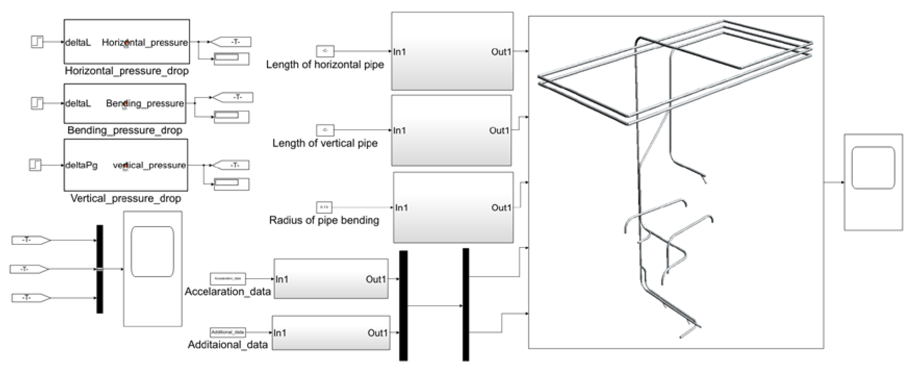
Physical modeling was carried out for each case of the pressure loss according to the pipeline of the BTS. To confirm the results of the pressure loss according to the input and to build the SILS model, modeling was carried out using MATLAB/Simulink. Figure 5 shows the pressure loss model of the BTS. Mathematical modeling was carried out for each case of the pressure loss according to the specifications and inlet pressure of the pipe. The detailed input specifications are listed in

Table 2. Specifications of pressure loss model of BTS.

Contents	Value (Unit)
Supply pressure	3.8 bar
Temperature	20 °C
Air density	1.17 kg/m3
Material density (apparent specific gravity)	2400 kg/m3 (barite)
Pipe diameter	0.13 m
Total length of horizontal pipe	127.9 m
Total length of vertical pipe	26.2 m
Angle of bending pipe	90°, 45°
Radius of bending pipe	0.75 m
Total length of pipe	161.6 m

.

2.2. Physical Modeling and Simulation of Bulk Storage Tank

In this study, component modeling was carried out to build the simulation models of the BTS. First, tanks were modeled for storing and transporting the bulk, such as the P-tank and surge tank. In addition, a subtank was constructed for emergencies, and valves and pumps for controlling the transportation of each material were modeled. This section describes the modeling of several representative components of the BTS.

2.2.1. Modeling of Bulk Storage Tank

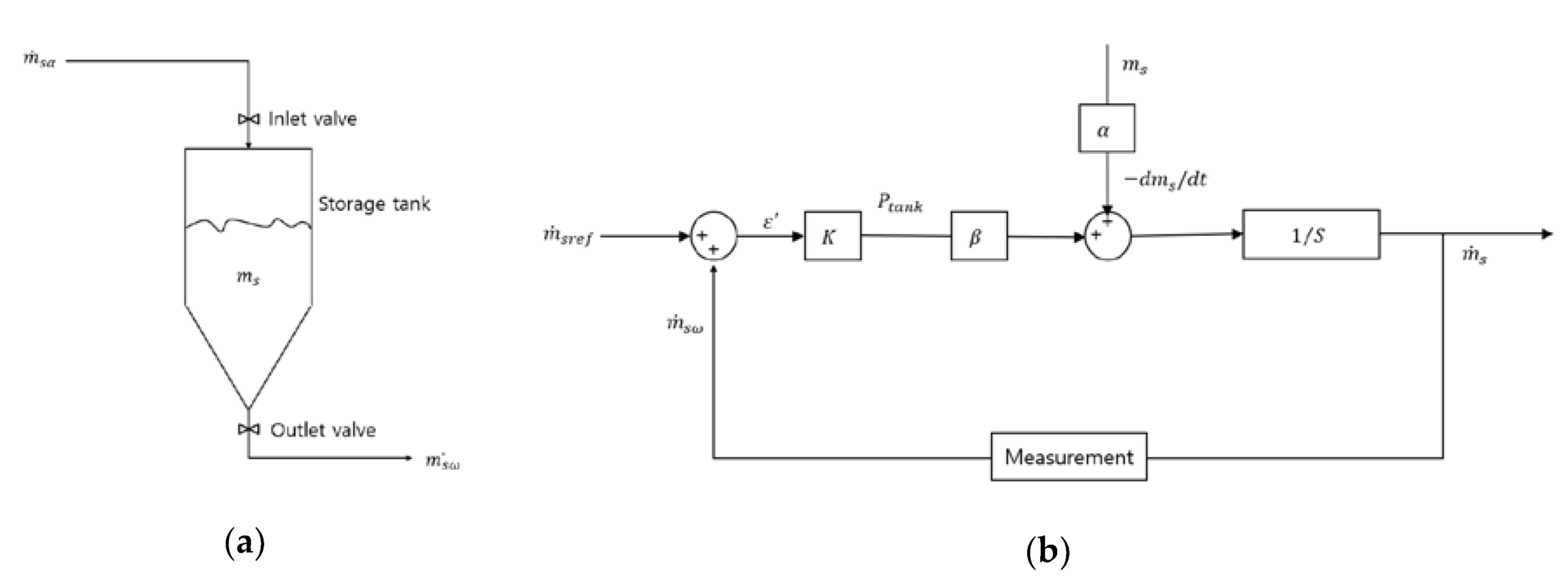
For pneumatic transport, the basic principle of analysis is based on the material balance of the transported solids. Several different situations could arise with regard to the control of the flow of solids. The macro approach to the control analysis will be considered first; then, the distributed models of the actual flow of solids will be explored in more detail. The simplest analogy of the system of the flow of solids is an equivalent system of the flow of liquids. Figure 6 shows an input–output situation from a bulk storage tank. In pneumatic transport, the delivery of a constant outflow of mass is a probable concern. If $m_s$ is the amount of solids in the storage or feeder unit, one can obtain the equation [25]

$$\frac{d{m}_s}{dt}={\dot{m}}_{s\alpha }-{\dot{m}}_{s\omega },$$

(6)

where $\alpha$ and $\omega$ refer to the initial and terminal states, respectively.

A method for maintaining a constant output is to set up a reference level in the feeder and maintain a constant tank pressure. The level or number of solids in the tank can be continuously measured

$${\epsilon }^{\prime }=m_{sref}-m_s,$$

(7)

where $m_{sref}$ is the reference amount of solids in the tank. The error can be set to be proportional to the inlet flow of solids so that ${\dot{m}}_{s\alpha }=\mathrm{K}{\epsilon }^{\prime }$.

The above scheme is only one type of control that can be employed. Various control schemes can be incorporated at this point in the analysis. The basic differential equation (Equation (8)) is expanded to yield

$$\frac{d{m}_s}{dt}+\mathrm{K}{m}_s=K{m}_{sref}-{\overline{\dot{m}}}_{so}.$$

(8)

The Laplace transform can be employed to obtain

$$m_s\left(\mathrm{s}\right)=\frac{1}{s+K}\left[K{m}_{sref}-{\overline{\dot{m}}}_{so}\left(s\right)+m_s\left(0\right)\right],$$

(9)

where s represents the Laplace transform notation. The signal flow diagram for this case is shown in Figure 6b.

2.2.2. Simulation of Bulk Storage Tank with Valve Signal

In this study, to build an integrated SILS model, components such as the surge tank, bulk storage tank, gate valve, and jet pump of the BTS were modeled. However, to verify the simulation model, the storage tank with inlet and outlet valves, jet pump, and active tank, which are essential elements of the BTS, were verified.

In this study, the BTS controls the tank level through valve control signals at the tank inlet and outlet. Figure 7a shows the control signal of the inlet valve of the P-tank. Figure 7b shows the level of the P-tank according to the signals of the inlet and outlet valves. Figure 7c shows the outlet valve control signal of the P-tank.

When the inlet valve of the P-tank is initially given by an open signal, the level of the P-tank increases linearly. When the maximum height of the P-tank reaches 5.1 m, the signal of the inlet valve automatically turns off. When the open signal of the outlet valve is given, the transfer of the bulk from the P-tank to the surge tank starts.

3. Results and Discussions

3.1. Simulation Verification of BTS Using Experimental Test Data

The results obtained using the pressure loss model of the BTS were compared with experimental test data. The test method was as follows, and the test environment is presented in

Table 3. Test environment for simulation.

Dry Bulb Temperature (°C)	Relative Humidity (%R.H.)
10 ± 1	20 ± 5

and

Table 4. Comparison of empirical data and simulation results.

Condition	Before Transferring	During Transferring	During Transferring	After Transferring
P-tank pressure	3.8	3.7	3.6	3.6
Surge tank pressure	0.2	0.5	1.5	1.8

.

• After filling the P-tank with the bulk, the air pressure was increased up to 3.8 bar.
• After checking the set pressure, the bulk transfer valve from the P-tank to the surge tank was opened.
• The pressure rise in the surge tank was checked through the monitoring panel of the bulk transfer control box.

The following test results were obtained at the Korea Marine Equipment Research Institute in South Korea. Figure 8 shows a land-based testbed for the BTS (left) and the piping and instrumentation diagram of the real testbed (right).

Figure 9 and

Table 5. Comparison of simulation and experimental results.

Type	Simulation Model Data	Test Data
Inlet pressure (bar)	3.8	3.8
Pipe diameter (m)	0.13	0.13
Pipe length (m)	161.57	161.57
Horizontal pipe length (m)	127.9	127.9
Vertical pipe length (m)	26.2	26.2
Bending pipe number (EA)	13	13
Outlet pressure (bar)	2.87	2.90
Error (%)	4.27

present the results of a comparison between simulation and test data. The simulation was performed under the same conditions as the test. The simulation of the pressure loss in Figure 9 was carried out using MATLAB/Simulink. Here, it was performed without the air booster. The input pressure supplied by the compressor started at 3.8 bar and rapidly decreased in the vertical pipe section. Then, in the horizontal and bending pipe sections, the decrease was relatively less (loss of 1.14 bar). Accordingly, an output pressure of 2.66 bar was obtained. The error rate of the pressure was confirmed to be 4.27%. The reason for the error is that in the case of bulk transfer in the physical world, two more phase transitions occur according to nonlinear factors. Multiple phases exist according to the classification of the bulk transfer characteristics. However, it is difficult to fully reflect the characteristics in the simulation model. In addition, the error can be attributed to the fact that the pipeline layout and the number of valves are not reflected in the simulation model.

In this study, case simulation was performed to observe the change in the pressure loss according to the specifications of the pipeline when designing the BTS. The simulation was performed by fixing the inlet pressure and the length of the entire pipe to 3.8 bar and 161.57 m, respectively.

Table 6. Case simulation parameters with test scenario.

Inlet Pressure (3.8 bar)	Horizontal Length of Pipe (m)	Vertical Length of Pipe (m)	Bending Pipe Number (EA)	Total Length (m)	Outlet Pressure (bar)
Case 1	127.94	26.17	13	161.57	2.66
Case 2	137.94	16.17	13	161.57	2.99
Case 3	117.94	36.17	13	161.57	2.32
Case 4	131.67	29.9	26	161.57	2.65
Case 5	124.21	29.90	26	161.57	2.41
Case 6	120.48	33.63	26	161.57	2.78
Case 7	135.40	18.71	26	161.57	2.28

Inlet pressure: 3.8 bar; Case 1: Simulation model; Case 2: Length of horizontal pipe = 10 m, length of vertical pipe = 10 m; Case 3: Length of horizontal pipe = 10 m, length of vertical pipe = 10 m; Case 4: Bending pipe number = 13 EA, length of vertical pipe = 3.73 m, length of vertical pipe = 3.73 m; Case 5: Bending pipe number = 13 EA, length of vertical pipe = 3.73 m, length of vertical pipe = 3.73 m; Case 6: Bending pipe number = 13 EA, length of vertical pipe = 7.46 m, length of vertical pipe = 7.46 m; Case 7: Bending pipe number = 13 EA, length of vertical pipe = 7.46 m, length of vertical pipe = 7.46 m.

lists some parameters of the pressure loss simulation of the BTS.

The case simulation of the pressure loss model was performed by entering the inlet pressure as 3.8 bar and specifying different variables for each case. Proper air pressure, piping layout design technology, and prescribed design guidelines are required to transport the bulk without clogging at the desired transport rate. In addition, the operating pressure and the amount of air determine the system cost. Therefore, an optimal design technology is required for the system.

Figure 10 shows the pressure loss according to the unit length of the vertical and horizontal pipes. When the length of the vertical pipe exceeds 103 m in the BTS design, the outlet pressure of 0 bar is no longer allowed to transfer the bulk under a theoretical background.

3.2. Simulation Optimization of BTS Using Genetic Algorithm

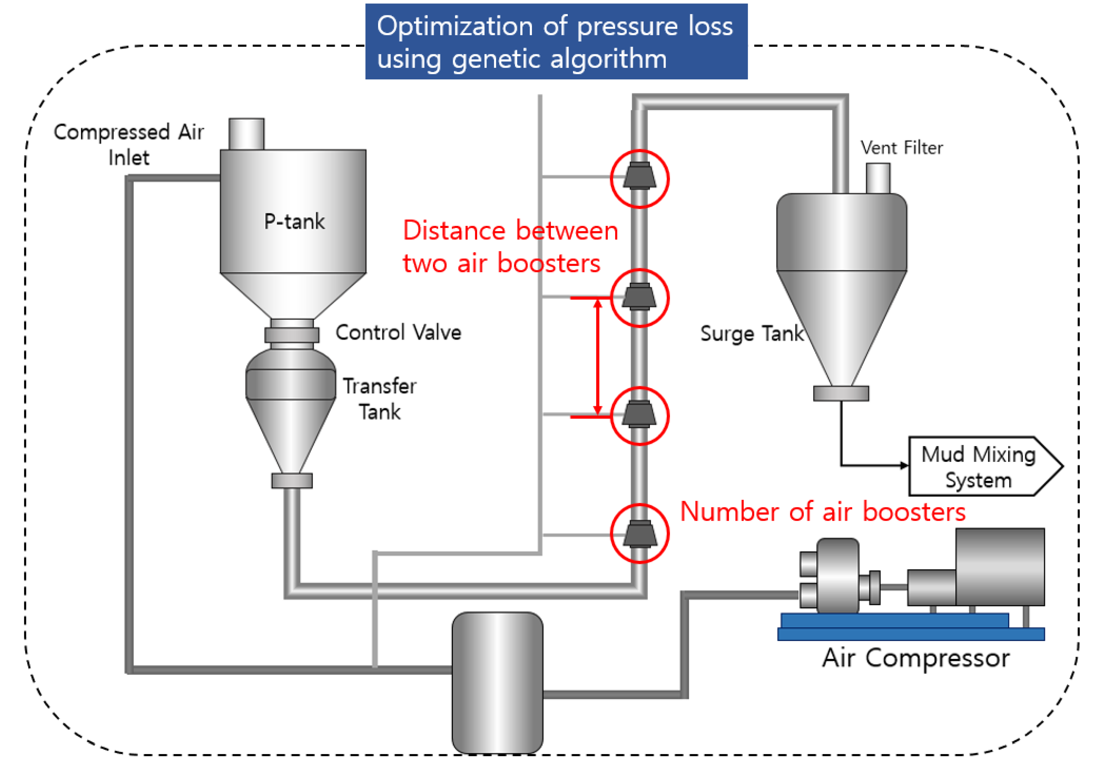
In this study, an air booster was installed to prevent clogging and equipment damage due to the pressure loss effect discussed in the previous section. The air booster minimized the pressure loss in the vertical pipe section where the pressure loss was high. A genetic algorithm was applied to optimize the number of boosters installed and the distance between them (Figure 11 and Figure 12). The optimization process was carried out using MATLAB/Simulink (version 2019b).

The pressure loss of the BTS was set as the objective function. The number of air boosters and the distance between them, which were to be optimized, were configured as variables. The pressure was measured in bars, and the installation distance was measured in meters.

Table 7. Genetic algorithm parameters.

Parameter	Value
Population size	2000
Number of generations	400
Goodness of convergence conditions	Proportion
Selection	Roulette
Reproduction (crossover ratio)	0.85
Probability of mutation	0.01
Crossover	One-point crossover
Function tolerance	$1.0\times {10}^{-6}$
Constraint tolerance	$1.0\times {10}^{-3}$

lists the set values for the parameters of the genetic algorithm. These values were set by focusing on the convergence of the fitness values.

In this study, considering the convergence of the goodness of fit and the performance of the computer, the population size was set to 2000 individuals and the number of generations was 400, which is 100 times the number of variables. The convergence condition for the goodness of fit was set proportionally. Selection refers to the process of selecting parents from a population for mating according to the fitness value after all the individuals in the population have been evaluated for fitness. The selection types are roulette selection, ranking-based selection, and tournament selection. Roulette was selected in this case. Crossover is an operator that uses the advantages of two chromosomes to make a better chromosome, and crossover types include one-point crossover, two-point crossover, and uniform crossover. One-point crossover was selected. Reproduction (crossover ratio) is a variable that determines how often crossover occurs and is generally maintained between 80% and 90%. We selected the ratio as 0.85. The probability of mutation is a variable that determines how often a gene is altered and is set to a very small value in genetic algorithms, as the probability of mutation in the natural world is very rare. It was selected as 0.01 in our study. Figure 13a,b shows the results of the genetic algorithm.

Figure 13a shows the best fitness, best function value, and number of iterations in each generation. Figure 13b shows the best individual and the vector item of the individual as the best-fit function value in each generation.

Table 8. Comparison of pressure loss along air booster positions.

	${\mathit{y}}_1\left(\mathbf{m}\right)$	${\mathit{y}}_2\left(\mathbf{m}\right)$	${\mathit{y}}_3\left(\mathbf{m}\right)$	${\mathit{y}}_4\left(\mathbf{m}\right)$	Inlet Pressure (bar)	Outlet Pressure (bar)
Case 1	N/A	N/A	N/A	N/A	3.80	3.66
Case 2	N/A	N/A	N/A	N/A	3.88	2.99
Case 3	6.00	9.00	12.00	15.00	3.80	3.33
Case 4	5.85	12.45	16.45	18.45	3.80	3.53

lists the pressure changes for the four cases of the vertical section of the BTS. The four cases are listed in Table 8, and they represent the installation positions of the air boosters.

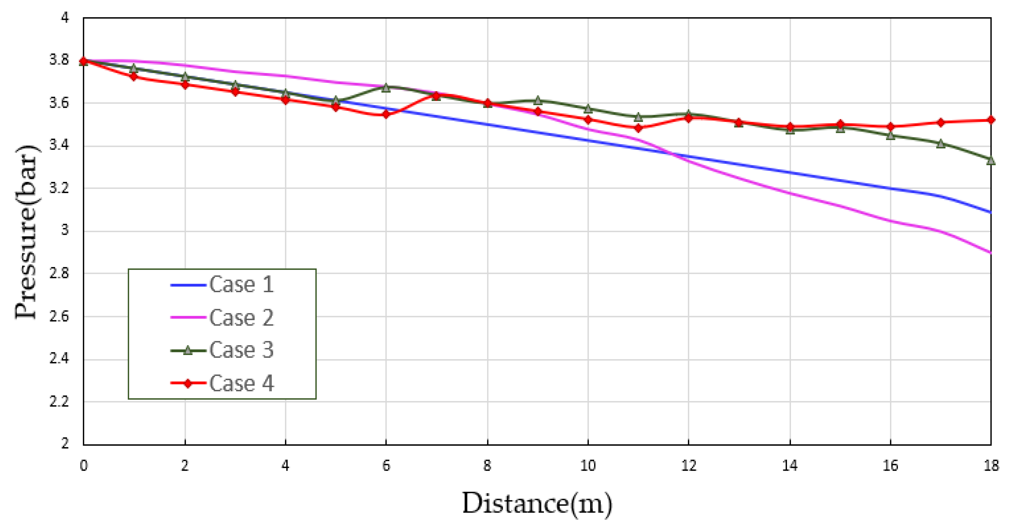
Figure 14 shows the pressure change in the vertical pipe section for Case 1–4. The four cases show the optimization of the distance of the air boosters. Case 1 represents a pressure change in the simulation model, whereas Case 2 represents a pressure change in the experimental test. Case 3 represents a pressure change when installing the air boosters at equal intervals, whereas Case 4 represents a pressure change when applying the genetic algorithm to the air boosters. In Case 1, the final pressure is 2.87 bar, which is a linear decrease of 0.93 bar from 3.80 bar. In Case 2, the final pressure is 2.90 bar, which nonlinearly drops from 3.80 bar. When the air booster is installed at equal intervals (Case 3), the outlet pressure is 3.33 bar. When the air booster installation positions are adjusted by applying genetic algorithm optimization (Case 4), the outlet pressure is 3.53 bar, which is compensated as one moves away from the installation position point ($y_i$).

4. Conclusions

In offshore drilling systems, the localization rate of equipment is less than 20%, and the monopoly of a few foreign conglomerates over the equipment is intensifying. To break this monopoly, active technology development and market entry strategies are required. Recently, the demands of ship owners for drilling systems have diversified and the complexity of integrated systems has increased. In this study, the overall pressure loss of the BTS is modeled and simulated. Real test data and simulation results are compared and analyzed to verify the simulation model. In addition, an air booster is installed and used to compensate for the pressure loss and thereby prevent clogging. A genetic algorithm is used to determine the number of air boosters required to optimize pressure loss and the distance between the boosters. The major results obtained are as follows.

(1)

A BTS was modeled and simulated to mitigate the clogging problem frequently encountered in transfer pipelines.

(2)

A numerical analysis was performed to optimize the pressure loss, to improve productivity. Pressure loss was modeled, and a pipeline was simulated to prevent the blockage problem in the BTS, and an empirical test was performed to validate the simulation model for comparative verification.

(3)

The simulation verification of the BTS indicated that the error rate was 4.27%. The reliability of the model can be further increased by continuously testing and upgrading the model. Additionally, four cases were simulated based on the verified model.

(4)

The pressure loss was optimized by applying a genetic algorithm to the air boosters that compensate for the pressure loss. The number of air boosters required and the distance between them were obtained. The optimized air booster compensated the pressure loss for approximately 0.54 bar.

(5)

To expand the applicability of the simulation model, further systematic experiments should be performed in the future for the saturation of the HILS.

Moreover, based on the optimized BTS, it is expected that a modeling and simulation application method can be developed for various facilities in offshore plants, and the optimized BTS is expected to contribute to the reduction of uncertainty and minimization of maintenance and repair costs during operation. It is also expected to contribute to the advancement of high-value fields such as construction, commissioning, installation, maintenance, and equipment localization improvement.

References

- Peterman, C.P.; Goldsmith, R.G.; Mott, K.C.; Danna, J.M.; Pelata, K.L.; Colvin, K.W. Offshore Drilling System. U.S. Patent 09/276,404, 4 December 2001. [Google Scholar]
- Wojtanowicz, A.K. Testing Protocol and Breakeven Cost Analysis of Mud Dewatering for Closed-loop Drilling System. J. Can. Pet. Technol. 1997, 16, 3. [Google Scholar] [CrossRef]
- Tsuji, Y.; Morikawa, Y. LDV measurements of an air-solid two-phase flow in a horizontal pipe. J. Fluid Mech. 1982, 120, 385–409. [Google Scholar] [CrossRef]
- Tsuji, Y. Multiscale modeling of dense phase gas-solid flow. Chem. Eng. Sci. 2007, 62, 3410–3418. [Google Scholar] [CrossRef]
- Theuerkauf, J. Application of discrete element method simulations industry. In Proceedings of the 7th International Conference for Conveying and Handling of Particulate Solids (CHoPS), Friedrichshaven, Genrmany, 10–13 September 2012. [Google Scholar]
- Klinzing, G.E. Historical Review of Pneumatic Conveying. KONA Powder Part. J. 2018, 35, 150–159. [Google Scholar] [CrossRef] [Green Version]
- Kuang, S.B.; Chu, K.W.; Yu, A.B.Z.; Zou, S.; Feng, Y.Q. Computational investigation of horizontal slug flow in pneumatic conveying. Ind. Eng. Chem. Res. 2008, 47, 470–480. [Google Scholar] [CrossRef]
- Kuang, S.B.; LaMarche, C.Q.; Curtis, J.S.; Yu, A.B. Discrete particle simulation of jet-induced cratering of a granular bed. Powder Technol. 2013, 239, 319–336. [Google Scholar] [CrossRef]
- Lecreps, I.; Sommer, K.; Wolz, K. Stress states and porosity within horizontal slug by dense-phase pneumatic conveying. Part. Sci. Tech. 2009, 27, 297–313. [Google Scholar] [CrossRef]
- Levy, A. Two-fluid approach for plug flow simulations in horizontal pneumatic conveying. Powder Tech. 2000, 112, 263–272. [Google Scholar] [CrossRef]
- Sanchez, L.; Vasquez, N.A.; Klinzing, G.E.; Dhodapkar, S. Evaluation of models and correlations for pressure drop estimation indense phase pneumatic conveying and an experimental analysis. Powder Tech. 2005, 153, 142–147. [Google Scholar] [CrossRef]
- Ryu, M.; Jeon, D.S.; Kim, Y. Prediction and improvement of the solid particles transfer rate for the bulk handing system design of offshore drilling vessels. Int. J. Nav. Archit. Ocean. Eng. 2015, 7, 964–978. [Google Scholar] [CrossRef] [Green Version]
- Mills, D. Optimizing pneumatic conveying. Chem. Eng. 2000, 107, 74–80. [Google Scholar]
- Mills, D. Pneumatic Conveying Design Guide, 2nd ed.; Butterworth-Heinemann, Elsevier: Oxford, UK, 2004. [Google Scholar]
- Mills, D.; Jones, M.G.; Vijay, K. Handbook of Pneumatic Conveying Engineering. Dekker Mechanical Engineering; CRC Press: New York, NY, USA, 2004. [Google Scholar]
- Sarhadi, P.; Yousefpour, S. State of the art: Hardware in the loop modeling and simulation with its applications in design, development and implementation of system and control software. Int. J. Dynam. Control. 2015, 3, 470–479. [Google Scholar] [CrossRef]
- Jing, W.; Yulun, S.; Wendong, L.; Ji, G.; Monti, A. Development of a Universal Platform for Hardware In-the-Loop Testing of Microgrids. IEEE Trans. Ind. Inform. 2014, 10, 2154–2165. [Google Scholar]
- Bouscayrol, A.; Lhomme, W.; Delarue, P.; LemaireSemail, B.; Aksas, S. Hardware-in-the-loop simulation of electric vehicle traction systems using Energetic Macroscopic Representation. In Proceedings of the IECON 2006—2nd Annual Conference on IEEE Industrial Electronics, Paris, France, 6–10 November 2006; pp. 5319–5324. [Google Scholar]
- Lauss, G.F.; Faruque, M.O.; Dufour, C.; Viehweider, A.; Langston, J. Characteristics and Design of Power Hardware-in-the Loop Simulations for Electrical Power Systems. IEEE Trans. Ind. Electron. 2016, 63, 406–417. [Google Scholar] [CrossRef]
- Ren, W.; Steurer, M.; Baldwin, T.L. Improve the stability and the accuracy of power hardware-in-the-loop simulation by selecting appropriate interface algorithms. IEEE Trans. Ind. Appl. 2008, 44, 1286–1294. [Google Scholar] [CrossRef]
- Li, H.; Steurer, M.; Shi, K.L.; Woodruff, S.; Zhang, D. Development of a unified design, test, and research platform for wind energy systems based on hardware-in-the-loop real-time simulation. IEEE Trans. Ind. Electron. 2006, 53, 1144–1151. [Google Scholar] [CrossRef]
- Lee, S.-J.; Kwak, S.-K.; Kim, S.-H.; Jeon, H.-J.; Jung, J.-H. Test platform development of vessel’s power management system using hardware-in-the-loop simulation technique. J. Electr. Eng. Tech. 2017, 12, 2298–2306. [Google Scholar]
- Hwang, J.T.; Hong, S.Y.; Kwon, H.W.; Lee, K.; Song, J.H. Dual Fuel Generator Modelling and Simulation for Development of PMS HILS. J. Korea Inst. Inf. Commun. Eng. 2017, 21, 613–619. [Google Scholar]
- Lee, K. Software-In-the-Loop based Power Management System Modelling & Simulation for a Liquefied Natural Gas Carrier. J. Korea Inst. Inf. Commun. Eng. 2017, 21, 1218–1224. [Google Scholar]
- Klinzing, G.E.; Rizk, F.; Marcus, R.; Leung, L.S. Pneumatic Conveying of Solids—A Theoretical and Practical Approach; Particle Technology Series; Springer: Berlin, Germany, 2010; pp. 4–33. [Google Scholar]
- Desai, N. Investigations in Gas-Solid Multiphase Flows. Ph.D. Thesis, North Carolina State University, Raleigh, NC, USA, 2003. [Google Scholar]
- Zenz, F.A.; Othmer, D.F. Fluidization and Fluid Particle Systems; Reinhold Publishing Coporation: New York, NY, USA, 1960. [Google Scholar]
- Nied, C.; Hauth, D.; Sommer, K. Stress States and Pressure Loss in Pneumatically Conveyed Spatially Confined Single Plugs; ICBM: Newcastle, Australia, 2011. [Google Scholar] [CrossRef]
Figure 1.
Schematic of mud circulation system, including MTS and BTS.
Figure 2.
Schematic of BTS inside hold of drillship.
Figure 3.
Conceptual diagram and pressure loss configuration of BTS.
Figure 4.
Piping and instrumentation diagram (P&ID) of BTS and three-dimensional pipeline modeling of proposed system.
Figure 5.
Physical modeling of BTS for pressure drop.
Figure 6.
Physical modeling of storage tank: (a) input/output from storage tank; (b) signal flow diagram for storage tank.
Figure 7.
Storage tank dynamics with on/off valve signal: (a) inlet valve on/off signal of storage tank; (b) storage tank level simulation according to changing valve signals; (c) outlet valve on/off signal of storage tank.
Figure 8.
Land-based testbed for BTS (left) and piping and instrumentation diagram of real testbed (right).
Figure 9.
Comparison of simulation and experimental results.
Figure 10.
Pressure drop comparison between horizontal and vertical pipes.
Figure 11.
Optimal positions of air boosters for pressure loss minimization.
Figure 12.
Schematic of genetic algorithm.
Figure 13.
Results of genetic algorithm: (a) fitness value; (b) current best individual.
Figure 14.
Vertical pressure loss simulation of BTS for different cases.