Sediment Morphology and the Flow Velocity Field in a Gully Pot: An Experimental Study


1
Water Management Department, Faculty of Civil Engineering and Geosciences, Delft University of Technology, 2628 CN Delft, Zuid-Holland, The Netherlands
2
Partners4UrbanWater, 6532 ZV Nijmegen, Gelderland, The Netherlands
3
Experimental Facility Support Department, Unit Hydraulic Engineering, Deltares, 2629 HV Delft, Zuid-Holland, The Netherlands
4
Civil and Environmental Engineering Department, Faculty of Engineering, Norwegian University of Science and Technology, 7491 Trondheim, Trøndelag, Norway
*
Author to whom correspondence should be addressed.
Water 2020, 12(10), 2937; https://doi.org/10.3390/w12102937
Submission received: 24 September 2020
/
Revised: 15 October 2020
/
Accepted: 18 October 2020
/
Published: 21 October 2020
(This article belongs to the Special Issue Physical Modelling in Hydraulics Engineering)
Abstract
:Urban runoff (re)mobilises solids present on the street surface and transport them to urban drainage systems. The solids reduce the hydraulic capacity of the drainage system due to sedimentation and on the quality of receiving water bodies due to discharges via outfalls and combined sewer overflows (CSOs) of solids and associated pollutants. To reduce these impacts, gully pots, the entry points of the drainage system, are typically equipped with a sand trap, which acts as a small settling tank to remove suspended solids. This study presents data obtained using Particle Image Velocimetry (PIV) and Laser Doppler Anemometry (LDA) measurements in a scale 1:1 gully to quantify the relation between parameters such as the gully pot geometry, discharge, sand trap depth, and sediment bed level on the flow field and subsequently the settling and erosion processes. The results show that the dynamics of the morphology of the sediment bed influences the flow pattern and the removal efficiency in a significant manner, prohibiting the conceptualization of a gully pot as a completely mixed reactor. Resuspension is initiated by the combination of both high turbulent fluctuations and high mean flow, which is present when a substantial bed level is present. In case of low bed levels, the overlaying water protects the sediment bed from erosion.
Keywords:
urban drainage; gully pot; hydraulics; multiphase flow; PIV; SPIV; LDA; stereo photography; 3D printing1. Introduction
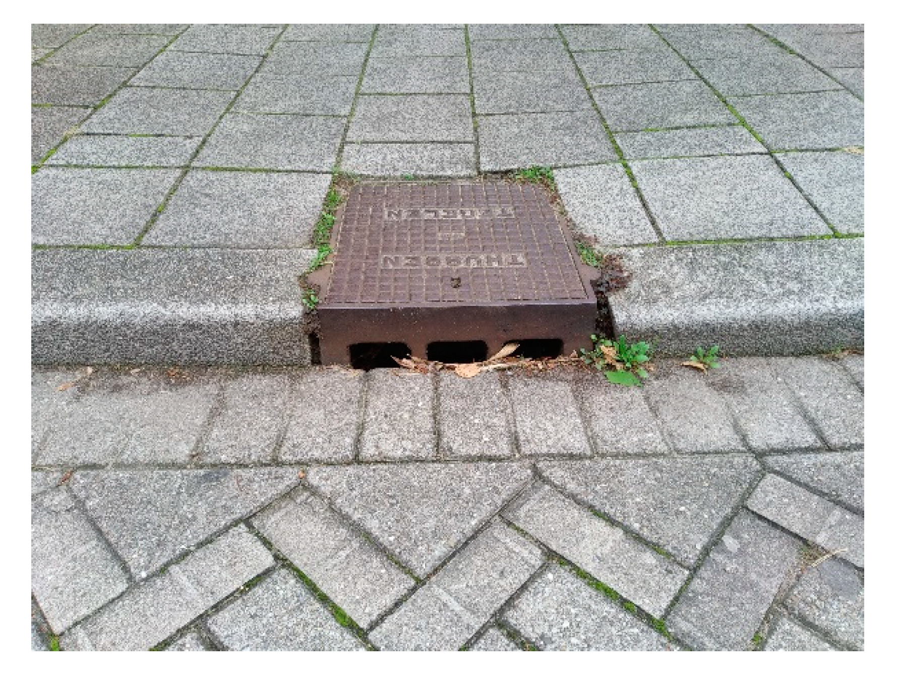
Urban drainage systems are meant to remove runoff from urban areas. Runoff contains suspended solids, which are (re)mobilised from the street surface by raindrop impact [1]. Accumulation of these solids in urban drainage systems result in a reduction of the hydraulic capacity ([2,3]), as they contain pollutants, pose a risk for the water quality of receiving water bodies (e.g., [4,5,6]). To reduce these adverse effects gully pots, the entry points of the drainage system (Figure 1), are usually equipped with a sand trap that acts as such an interceptor. Consequently, gully pots have to fulfil two objectives: (i) transport runoff from the street surface to the drainage system and (ii) removal of solids. From the second perspective, a gully pot can be seen as a small settling tank.
The sediment bed in a gully pot grows over time, which can eventually block the outlet pipe of the gully pot. A blocked outlet can induce flooding during a rainfall event [7] which may pose health risks [2,8]. Therefore, municipalities regularly clean out gully pots. This is done once or twice a year in urban areas [9,10] and two to four times a year at vulnerable locations, such as market places or shopping areas [9].
Post et al. [7] monitored the sediment build-up over a 15 months period in ~300 gully pots and concluded that up to ~5% of these gully pots got clogged due to increasing sediment bed levels. The sediment bed level in the remaining ~95% reached a stable level after a few months, implying that in most gully pots the removal efficiency strongly decreases over time and the solids loading to the downstream drainage system strongly increases. Rietveld et al. [11], who monitored and modelled the accumulation rate of solids in 400 gully pots, proved that the sediment bed level and the hydraulics significantly affect the removal efficiency.
Butler and Karunaratne [12] studied the removal efficiency of gully pots employing lab experiments and concluded that the gully pot can be approximated as a completely mixed reactor. Based on these experiments, the removal efficiency was modelled as the trade-off between the settling velocity and the surface loading:
in which ws is the settling velocity and A is the free water surface of the gully pot. Rietveld et al. [13] confirmed the validity of this equation by means of lab experiments. This validity though is limited to the initial removal efficiency of gully pots with an outlet at the opposite side from the inlet only. As soon as the sand trap gets filled, the removal efficiency drops rapidly. This decrease is not described by the Butler and Karunaratne equation, therefore the model does not perform well for (partially) filled sand traps. In addition, equation 1 models the gully pot hydraulics solely by the surface loading, implicitly assuming complete mixing. [7,13] show that the outlet position does affect the removal efficiency of gully pots, thereby suggesting that the assumption of complete mixing is not valid. Therefore, information on the flow pattern and its interaction with the sediment bed is required to understand the settling and erosion processes and to improve the efficiency models eventually.
Yang et al. [14] simulated the flow and removal of solids in a gully pot by means of Computational Fluid Dynamics (CFD). The removal efficiency was validated by some physical tests performed by Tang et al. [15] (since only a few grams of sediment were used in these tests, the reduction of the removal efficiency due to an increasing sediment bed level, was not studied), which showed that the CFD model provided acceptable results for particles ≥250 µm, while it overestimated the efficiency for smaller particles. The flow pattern of their CFD model was validated by the flow velocity measurements of Howard et al. [16]. However, the latter modelled a sump with a horizontal inlet, which results should not have been extrapolated to gully pots with a vertical impinging jet. Faram and Harwood [17] also modelled the removal efficiency of gully pots and validated the results with a few physical tests of the removal efficiency; no validation of the velocity fields was reported.
A quantification of the relation between parameters such as the gully pot geometry, discharge, sand trap depth, and the flow pattern is required, to understand their effect on the settling and erosion processes in a gully pot. This study presents the results from (Stereo) Particle Image Velocimetry [18] and Laser Doppler Anemometry measurements [19] on the flow patterns in a gully pot. These results may be used to validate CFD simulations of the hydraulics and the water–solids interaction a gully pot.
2. Materials and Methods
2.1. Experimental Setup
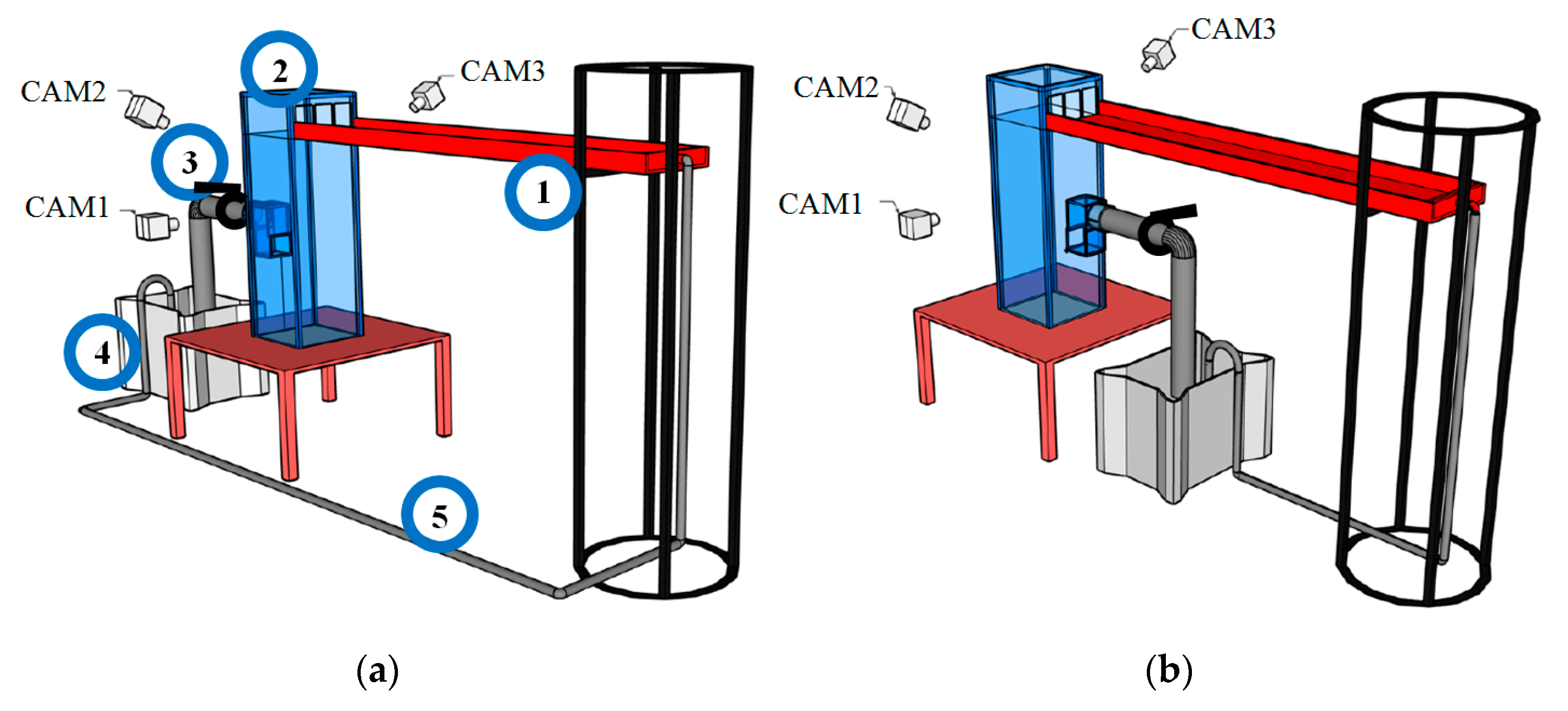
Figure 2 shows the experimental setup, which was used to mimic the flow pattern in a gully pot. The 1:1 scale gully pot, which is part of this setup, is also used by Rietveld et al. [13] and is constructed using transparent material (PMMA, also known as acrylate) to ensure optical access.
The water in the setup is discharged into an aluminium canal (with a slope of ~1%) and flows towards the gully pot. This gully pot has a side inlet, in line with the predominant type applied in The Netherlands, and is mounted with a height-adjustable bottom to mimic a range of sand trap depths as applied in practice. The top of the gully pot is convertible to ensure accessibility and for changing the relative position of inlet and outlet (see Figure 2b). A butterfly valve is mounted in the outlet pipe of the gully pot, which opening is adjustable to control the water level in the gully pot independent from the discharge. The water level was set at the top of the outlet pipe. The water ends up in the reservoir and is recirculated by a pump via a hose to the canal. The hose contains a ball valve and a flow meter, which are used to regulate the discharge through the system.
2.2. PIV
The PIV equipment consists of tracer particles, laser (optics), and camera(s). The laser illuminates the tracer particles in a plane in the gully pot. The camera captures images of the tracer particles and the flow velocity is obtained by dividing the displacement of the tracer particles in two consecutive images by the time interval between these two images. These calculations are performed with the software package DaVis 8.4.
2.2.1. Tracer Particles
The polyethylene tracer particles used had a density similar to water (0.99–1.01 kg/L) and a diameter of 90–106 µm, such that the particles followed the flow field closely (Stokes number < 1). The water originating from the gully pot inlet impinges on the water surface in the gully pot, causing air entrainment. The resulting bubbles reflect the laser light and distort the images. Therefore, fluorescent (orange) tracer particles and a camera with a colour filter were used. The filter removed the scattered light originating from the air bubbles and allowed the camera to capture the light from the illuminated fluorescent particles.
2.2.2. Laser
A pulsed Nd:YAG laser (Litron Nano) at 532 nm and a maximum output of 400 mJ is used to generate a laser bundle. The laser bundle is converted into a laser sheet with the use of lenses to illuminate the plane of interest.
2.2.3. Imaging
PIV estimates the displacement of tracer particles within a window (interrogation area) of two consecutive images with a known time interval. The velocity within the interrogation area (in this research an interrogation area of 32 × 32 for 2D flow fields and 48 × 48 pixels for 3D flow field with 50% overlap was used) was estimated by the displacement of the particles divided by the time interval between the two images. Universal outlier detection was used for vector validation [20]. The images were obtained by LaVision Imager MX cameras (sensor size of 2040 × 2048 pixels) with a Nikon Nikkor 28 mm f/2.8 lens (diaphragms used: f/4 and f/5.6).
Images were made with one camera for normal PIV to obtain a 2D flow field and with two cameras for stereo PIV (SPIV) to obtain a 3D flow field (a 2D flow field and its out of plane velocity component). 2D flow fields were obtained in vertical planes, while 3D flow fields were obtained in horizontal planes (Section 2.5.1). Camera position 1 in Figure 2 was used for the PIV flow fields and positions 2 and 3 for the SPIV flow fields. For the latter, the cameras were equipped with Scheimpflug adapters at the angle such that the horizontal Plane of Interest (POI) was in focus. The cameras were positioned at opposite sides of the gully pot at an angle of ~45 degrees. Acrylate water-filled prisms were mounted on the gully pot (Figure 3) to improve the imaging by reducing the refraction effects.
For each measurement 1000 double images at a sampling rate of 3 Hz were acquired to calculate the mean velocity field.
2.2.4. Camera Calibration
The camera calibration for each plane is performed with a calibration plate. The laser sheet was aimed at and aligned with the calibration plate. The known dimensions of the plate are used to calculate the reprojection parameters (i.e., the extrinsic and intrinsic camera parameters) and are eventually used to map the displacement of tracer particles in the camera images to real-world coordinates.
This type of calibration includes the refraction at the air/acrylate and acrylate/water interfaces, which improves the accuracy, but limits (reliable) measurements to the calibrated area. For PIV a specially designed calibration plate of 700 × 349 mm (just fitting in the gully pot) with circular markers every 10 mm was used and for the SPIV measurements a dual-level calibration plate with circular markers (LaVision, type 21) was used. The latter calibration plate is required to calculate the out of plane component of the velocity. The calibration for these SPIV measurements was further improved by self-calibration correction.
2.3. LDA
2.3.1. LDA Equipment
Laser Doppler Anemometry (LDA) measurements are performed to acquire information on the turbulent fluctuations, which might influence the resuspension. The LDA system (Figure 4) consists of four main components, namely a laser unit, two optical receivers, and an electronic signal processing unit. The He-Ne laser generates a continuous 5 mW beam, which is split into three beams: one main beam and two reference beams. The beams interfere at the focal point (~40 cm in this study). Reflections of the main beam on particles in this focal point interfere with the reference beams, and contain a frequency shift due to the Doppler effect. The two modulated beams are captured by the optical receivers and processed by the electronic signal processing unit. The latter converts the frequency of the modulated signal into a two-directional flow velocity. The third component can be obtained by rotating the system 90 degrees and focusing on the same measurement location.
Both the laser unit and the optical receivers were placed on a traverse system. These traverse systems were used to change the measurement location. The measurement location was verified with a calibration plate (similar to the one used for the PIV system) of 600 × 349 mm (just fitting in the gully pot) with circular markers.
2.3.2. LDA Post-Processing
The LDA measurements are used to study the turbulent fluctuations, which are defined as:
in which is the turbulent fluctuation, the mean velocity, and u the instantaneous velocity. This decomposition of the instantaneous velocity is commonly referred to as Reynolds decomposition. The mean velocity and variance are defined as:
The turbulent kinetic energy (TKE) is a measure of the amount of energy in the turbulent fluctuations and the turbulent intensity (TI) is a measure of the amount of energy in the turbulent fluctuations relative to the energy in the mean flow. These parameters are defined as [21]:
The kinetic energy is distributed over eddies of various length-scales. Energy is fed from the mean flow to the large eddies and cascades to the smallest eddies which are damped out by viscosity and eventually dissipate molecular movement (heat). This can be displayed by the energy spectrum, which is defined as the Fourier transform of the autocorrelation of the velocity fluctuations:
in which ω is the angular frequency, and ρ the normalised autocorrelation function. The timescale of the large turbulent structures, the integral time-scale, is defined as:
in which is specified as the time at which the correlation function is zero. In addition to the integral time-scale, a turbulent flow is characterised by the integral velocity-scale () and the integral length-scale (), which are defined as:
The dissipation of the kinetic energy (ε) at the smallest scale (Kolmogorov scale) is proportional to:
and in terms of these smallest scales:
in which ν is the kinematic viscosity, and and the Kolmogorov velocity- and length-scale, which are defined as:
The Taylor microscale can be found in between the integral and Kolmogorov scale. At this scale, the dissipation can be estimated by:
in which λ is the Taylor length-scale and is defined as:
In case of anisotropic turbulence, Equations (7)–(15) are defined for each direction separately, while in most cases isotropic turbulence is assumed and one value can be used. The kinetic energy is distributed over the three length-scales, which is usually displayed by the graphical representation of the energy spectrum versus the wavenumber. In case of a large mean flow compared to the turbulent fluctuations, the transformation from the angular frequency (in Equation (7)) to the wavenumber can easily be made via Taylor’s hypothesis. In the case of a highly turbulent flow, this is not possible, and the energy spectrum is expressed as energy contribution as a function of the (angular) frequency of the fluctuations [22]. The spectrum can mathematically be described by:
The presence of the power −5/3 can be used to validate whether real turbulence is measured.
2.4. Measurement Devices
2.4.1. Flowmeter
The flowmeter is a Fischer and Porter magnetic flowmeter, model D10d. The measurement range is 0 to 3.5 L/s. The uncertainty (95% confidence interval) of the device is estimated at ±1% of the full scale.
2.4.2. Thermometer
The water temperature changed during the experiments due to the friction in the recirculation system, influencing the viscosity of the water. The temperature of the water in the reservoir was measured during each experiment with a PT100rs thermometer. Since the temperature in the system was not entirely homogeneous, the uncertainty (95% confidence interval) is estimated at ±1 °C.
2.5. Test Conditions
2.5.1. Planes of Interest
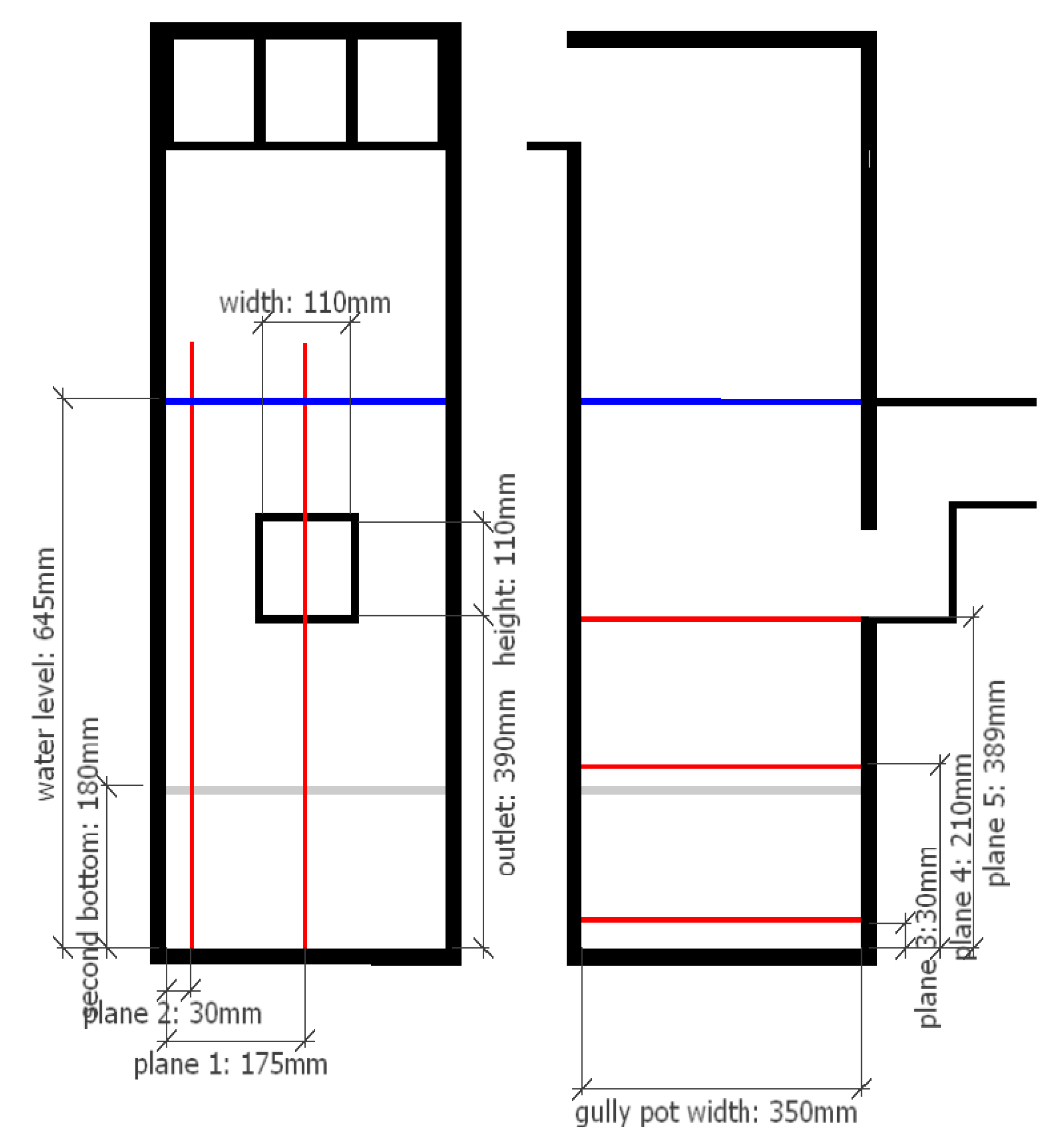
Five planes of interest (POIs) were selected for (S)PIV measurements, two vertical and three horizontal planes, which are shown in Figure 5. LDA measurements are only performed in plane 1, which is the plane of symmetry in the gully pot. The flow in plane 2 includes the effect of the gully pot wall. The flow in these planes (in particular, plane 1) should be mainly within rather than through the plane. Therefore, PIV measurements are performed for these planes (with the camera located at position 1 in Figure 2).
Planes 3 and 4 contain information on the flow field close to the gully pot’s (second) bottom. Plane 5 contains the contraction region of the flow due to the outlet. The flow directions in planes 3, 4, and 5 are both within and through the plane. Therefore, SPIV measurements are performed for these planes, which requires two cameras (camera positions 2 and 3 in Figure 2). These measurements involved a more extensive and precise positioning and calibration of the cameras (as described in Section 2.2.4).
2.5.2. Discharge
The water discharged into the gully pot represents runoff from rainfall events. The range of discharges tested in this study is 0.55 to 1.8 L/s, assuming a drained area of 150 m2 (which is a common value in The Netherlands), it represents a rainfall intensity between 13.2 and 43.2 mm/hour. Rainfall events causing the latter rain intensity over at least 10 min occur ~2 times a year in The Netherlands [23].
The study of Rietveld et al. [13] showed that for particles with a density of 2650 kg/m3 and a diameter ≥125 µm the initial removal efficiency is ≥73% at a discharge of 0.55 L/s. Lower discharges will result in even higher removal efficiencies and the evaluation of the removal efficiency at these discharges will provide limited additional data for model validation. Therefore, only the velocity fields at discharges ≥0.55 L/s is studied. This study focusses on the velocity field in a stationary situation, i.e., the effects of time-varying discharges and water levels on the flow field are not studied.
2.5.3. Sand Trap Depth
Gully pots come with a range of sand trap depths in practice; therefore, a (transparent) double bottom was added to evaluate its effect on the flow pattern. Two different depths were tested namely 0.21 and 0.39 m, equal to the depths tested by Rietveld et al. [13] for their effect on the removal efficiency.
2.5.4. Outlet Position
2.5.5. The Presence of a Sediment Bed
The flow pattern and its interaction with the sediment bed are the predominant dynamic processes influencing the accumulation of solids [13]. The visualisation and quantification of the flow pattern in the gully pot for an increasing sediment bed provide insight into the time dependency of the efficiency. However, (S)PIV and LDA cannot be used in combination with regular loose sand because of the interference of the sand particles with the tracer particles. Therefore, several artificial sediment beds were made, which represent the sand bed at various stages in the accumulation process. The development of these artificial sediment beds is described in Section 2.5.
2.6. Stereo Photography
Stereo photography, a method of combining two 2D images into a 3D object, was used to create a 3D model of the sediment bed at various stages. Figure 6a shows the setup for these measurements, which consisted of two PointGrey Blackfly cameras (sensor size of 2448 × 2048 pixels) with Fujinon HF12.5SA-1 12.5 mm f/1.4 lenses and an extra light source to improve the contrast in the images.
The stereo camera system was calibrated ([24,25]) with a calibration plate with a checkerboard pattern of 340 × 330 mm (squares of size 10 × 10 mm), which was submerged in the water in the gully pot (Figure 6a). This plate was placed in 15 different positions, varying in height and inclination to calibrate the cameras over the range of the sediment bed.
Since the cameras were located above the water surface, the water level height slightly influenced the reprojection parameters, due to the light diffraction at the water/air interface. Therefore, the water level during the calibration phase (Figure 7a) was adjusted to the same height as during the measurement phase (Figure 7b). The reprojection parameters were obtained with the Stereo Camera Calibrator App in MATLAB (version 2019a). The calibration resulted in a reproduction mean error of ~0.33 pixels.
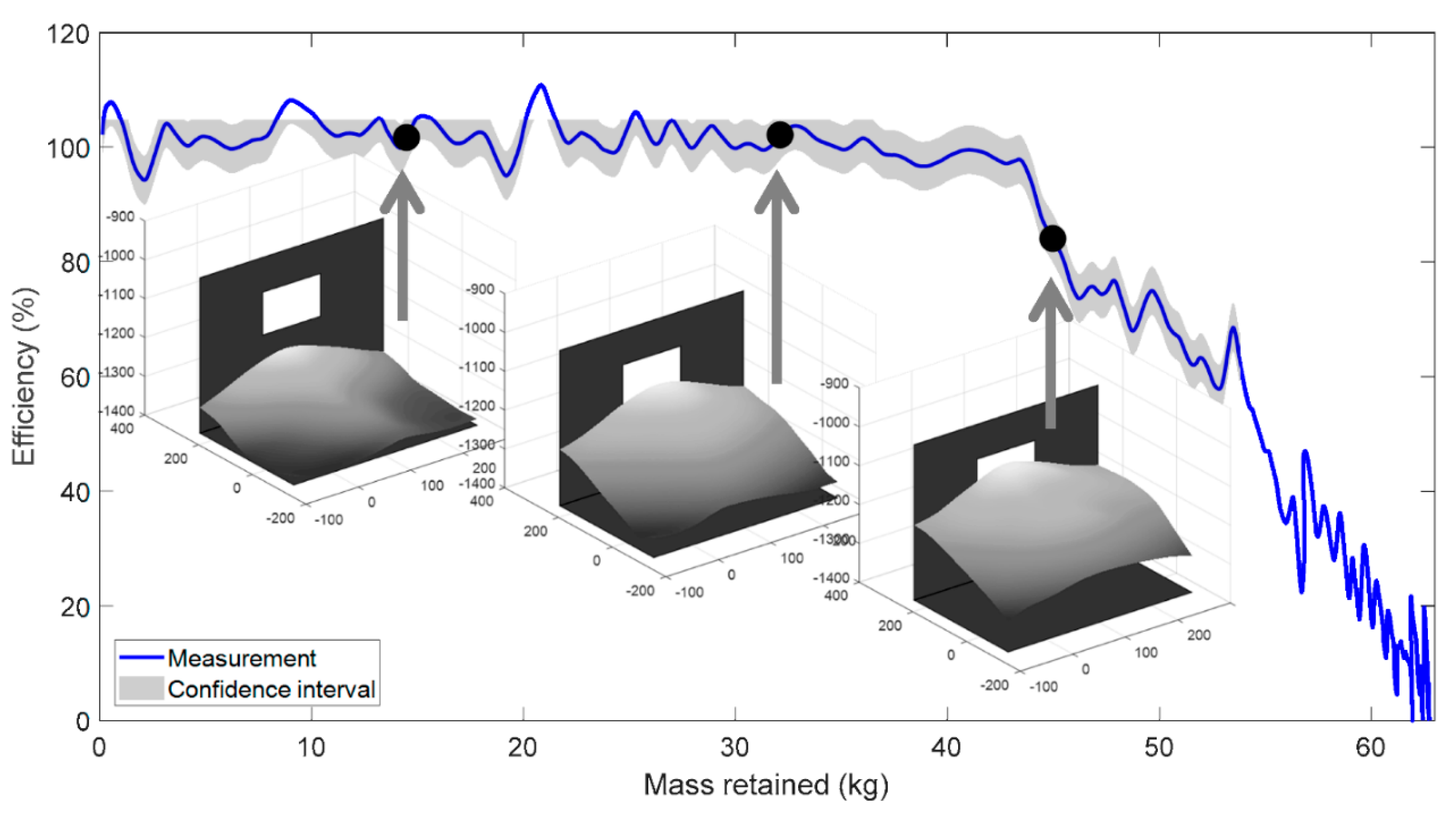
The recorded beds originated from a test at a discharge of 1.0 L/s, with the outlet at the back, a gully pot depth of 0.21 m, and sand with a D50 of 400 µm. The sediment accumulation occurred non-uniformly over the gully pot’s cross-section. The shape of the bed depends on the position of the impinging jets, the particle characteristics, and the gully pot geometry. In this test, all inflowing particles settle in the gully pot or in the siphon behind the gully pot initially, as indicated by the efficiency of ~100% in Figure 8. The efficiency curve shown in this figure originates from a removal efficiency test (by [13]) at the same conditions. The mass supply rate and the elapsed time of the current test were known, which made it possible to estimate the corresponding points in the graph at which the test was stopped to obtain the stereo photos; these points are indicated in the figure.
The first recording of the sediment bed was performed in this first phase. When the sediment bed gets close to the impinging jets, which originate from the gully pot inlet, the interaction between the sediment bed and the flow becomes apparent; particles can resuspend from the sediment bed and be transported out of the gully pot. The second recording was performed before and the third recording after this effect became apparent.
For each recording, the water inflow was carefully stopped, to prevent a collapse of the (loosely packed) sediment bed. The gully pot inlet was partially taken off (as can be seen in Figure 6a), small pebbles were added on top of the sediment bed to enhance the reference points and the 3D reconstruction of the bed (Figure 7b), and images were taken. The 3D reconstruction of the beds was performed with MATLAB and the beds were printed with a 3D printer using PLA. Figure 6b shows one of these beds, which was covered with a glued layer of sand (the same sand as originally used) for a realistic bed roughness.
3. Results and Discussion
3.1. Preliminary Observations in PIV and LDA Measurements
Figure 9a shows the velocity field in plane 1 obtained with PIV for the test with sand trap depth of 0.39 m, outlet at the back, and discharge 1.0 L/s. The local flow velocity and direction are indicated with the small arrows, while the colours indicate the mean velocity. The waterjets from the inlet impinge on the water, causing air entrainment. The air bubbles distort the laser sheet strongly, causing a lack of data in that area.
The flow around the impinging jet is directed upwards. This is thought to be caused by the multiphase character of the flow. The entrained air bubbles rise and on their way to the water surface, the water is pulled upwards, which is not captured in the CFD simulations of Yang et al. [14] and Faram and Harwood [17]. Avila et al. [26] could not simulate water, air, and sediment in one CFD simulation, but did show that air entrainment significantly influences the flow field in a CFD simulation and their results are more comparable to Figure 9a.
An overview of all PIV tests is provided in Appendix A.
It is concluded that the flow directions in the monitored plane are determined by two low-pressure zones, namely at the outlet and at the right of the impinging jet, and one high-pressure zone, namely at the left of the impinging jet, where the water leaves the impinging jet.
The maximum velocities can be found close to the impinging jet. The colour bar represents a velocity range of 0 to 0.10 m/s. From the perspective of sedimentation, the latter corresponds with the settling velocity of a sand particle with a diameter of ~630 µm (making use of the universal drag coefficient for spheres [27]).
To be able to study the local turbulence in more detail, next to the PIV measurements, LDA measurements are performed. In Figure 10a the mean velocities obtained by both techniques are shown and Figure 10b shows the residue between the two vector fields for validation. The residue vector is defined as:
A scalar is defined to represent to what extent the magnitude and the direction of the flow of both measurements are comparable. This scalar is defined as the inner product of the difference vector with the vector of the LDA measurement divided by the magnitude of the LDA measurement:
in which θ is the angle between the residue vector and the LDA vector. This scalar is shown in Figure 10c. The difference between the two measurements is relatively large for the seven measurements at the left side of the top row, which is the position where air bubbles are entrained in the water. It is not known what measurement technique provides the best results in this situation. At the other 52 positions, the flow direction and velocity are more comparable (absolute value of the difference scalar <0.02). Indicating that the complete rebuilding of the setup in between the PIV and LDA measurement series did not significantly affect the flow field. In the remainder of this article, the LDA measurements are used to study local turbulence and the PIV measurements are used to study the overall flow field.
To assess whether the turbulence is isotropic, the fluctuations in all three directions are needed. To obtain the third velocity component (the measurements in Figure 10 only contain two components), the LDA setup was rotated 90 degrees. These combined measurements were performed at 49 positions. Both measurements include the velocity in the z-direction, in which the turbulent fluctuations at all positions differ less than 30%. The standard deviations of the fluctuations relative to each other in the three directions are also small, namely less than 40%. Therefore, the assumption of isotropy is made in further calculations. This provides the means to calculate the TKE and TI based upon two components, by slight changes of the definitions. For the TKE the factor ¾ replaces the factor ½ to compensate for the third component, which effectively estimates the velocity fluctuations in the third direction by the two known directions:
The median (over all data points) of the turbulence intensity is 1.3, meaning that in most cases most energy is in the turbulence instead of in the mean flow, and therefore Taylor’s hypothesis on frozen turbulence does not hold. The impinging jets induce a highly turbulent flow, in particular in their close proximity as can be seen by the TKE as displayed in Figure 10b.
In Figure 11, the power spectrum is represented versus the frequency. The power −5/3 dependency is visible, indicating that there is turbulence indeed. The two velocity components show a similar power spectrum, and could also be displayed as one spectrum since isotropy was already assumed.
Since, LDA and PIV measurements cannot be combined with suspended solids, the influence of suspended particles, which are present in the water in field conditions, on the flow pattern is excluded. This implies that, at locations with a high suspended solids concentration (i.e., close to the bottom or the sediment bed), the measured turbulent fluctuations in the sediment-free situation represent the upper limit of its intensity compared with field conditions.
3.2. The Effect of the Sediment Bed
Gully pots get progressively filled due to their removal of solids from runoff. Rietveld et al. [13] observed that the removal efficiency is initially relatively constant, resulting in a steady build-up of the sediment bed. The build-up rate changes once a substantial bed level is reached, resulting in additional throughflow of sediment. The flow pattern is the driver of these processes.
Three artificial sediment beds were made, as described in Section 2.5, to visualise the interaction of the sediment bed with the flow pattern. These artificial beds represent the sediment at various stages for one condition, namely a discharge of 1.0 L/s, a gully pot with the outlet at the back, a depth of 0.21 m, and sand with a D50 of 400 µm. Other conditions give rise to other morphologies.
Figure 12 shows that, due to an increasing sediment bed level, the flow velocity close to the sediment bed increases, in particular close to the outlet. This is also the location where it was visually observed that the accumulation rate decreased and erosion took place [13], which started in between the situation of Figure 12c,d. In Figure 12c, the flow velocity increases to ~0.10 m/s, which is already larger than the settling velocity of sand particles of 400 µm. In Figure 12d, flow velocities up to ~0.15 m/s are present. It is assumed that even higher flow velocities are present close to the outlet, but these are in this situation optically obscured by air bubbles and therefore could not be quantified using PIV.
While the flow velocity strongly increases due to an increasing sediment bed level, the flow directions stay relatively constant: the stagnant zone at the top right and a split between the area at the left and right of the impinging jet. While the flow at the left is mostly pointed towards the outlet, the flow at the right is mainly pointed towards the impinging jet. The only change is the sediment bed that replaces the stagnant zone at the bottom left of Figure 12a.
Figure 12 shows that the jets impinge on the water in the middle of the gully pot and the x-direction of the flow close to the jets is towards the left (i.e., towards the outlet). Therefore, the sediment bed is thickest close to the outlet. In Figure 12b, the flow velocity close to the bed is still relatively low and is therefore of relatively less importance for the shape of the bed than the position of the impinging jets and the high flow velocities close to the jet. In later stages, Figure 12c,d show the flow velocity close to the sediment bed is in the same order of magnitude as the settling velocity of the sediment; the sediment can therefore easily move over the bed as bed load. This causes the dip in the bed shape in Figure 12d.
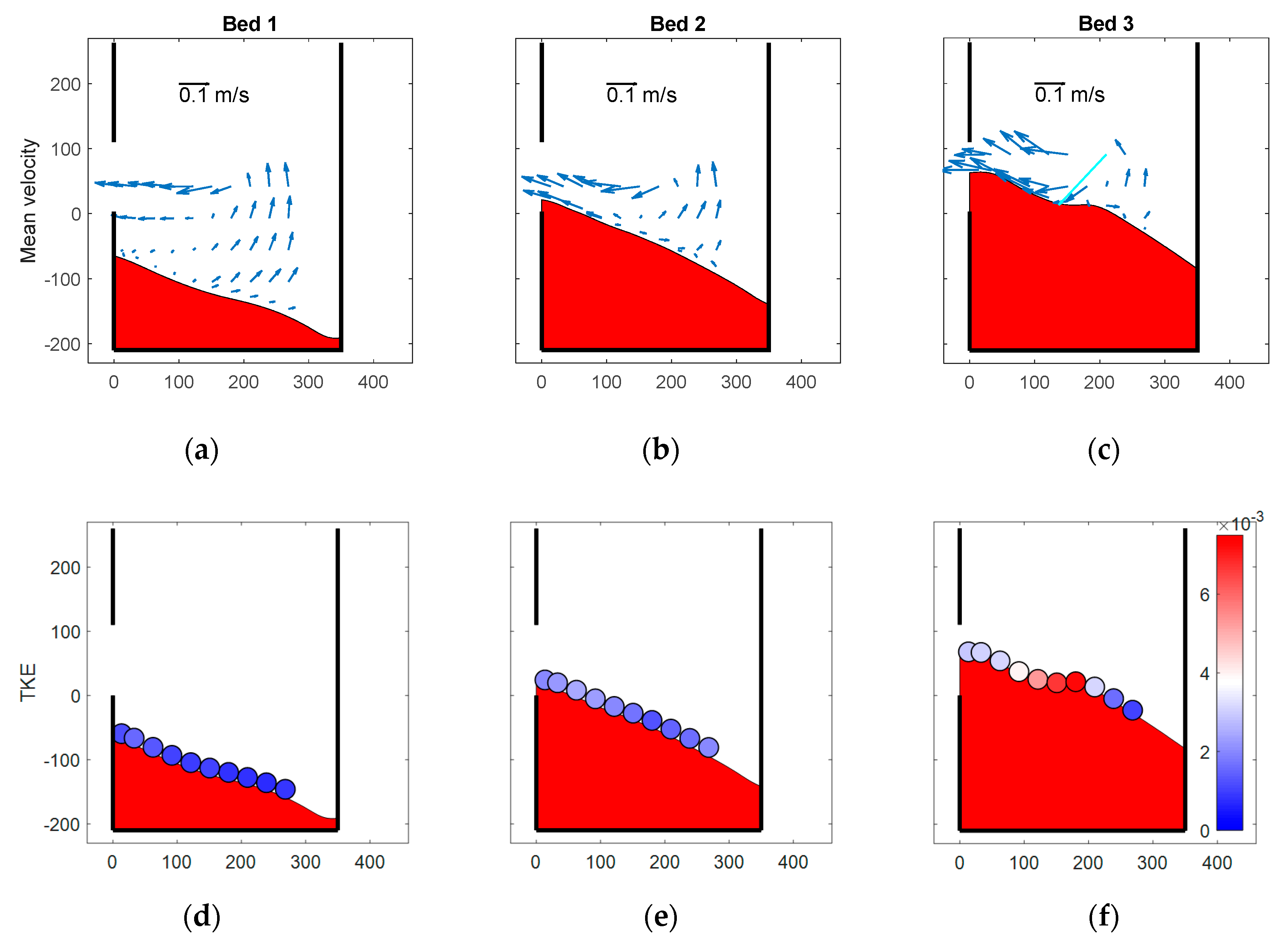
The velocities in Figure 12 represent mean velocities (averaged over 1000 frames captured at 3 Hz). Figure 13 shows the results of the LDA measurements, providing data on the mean velocity and turbulent fluctuations. The measurements for bed 3 contain an outlier in the mean velocity data, which is shown in another colour. This outlier is most likely due to air entrainment.
The TKE close to the bed reaches a maximum in the situation with the highest bed level, in particular in the region where the mean flow splits to the left and the right. This splitting point might change over time and give rise to a high TKE. The area close to the outlet is subjected to a lower TKE, but higher mean velocities. Since this is the area where resuspension was observed, it is concluded that the combination of the mean flow and the turbulence is required for local resuspension, and not the turbulence on its own.
In the case of lower bed levels, both the mean flow and turbulent fluctuations close to the bed are damped. This result confirms the conclusion of [28] that the overlaying water depth protects the sediment bed from the impact of the impinging jets as long as the sand trap is sufficiently deep.
3.3. The Effect of the Discharge
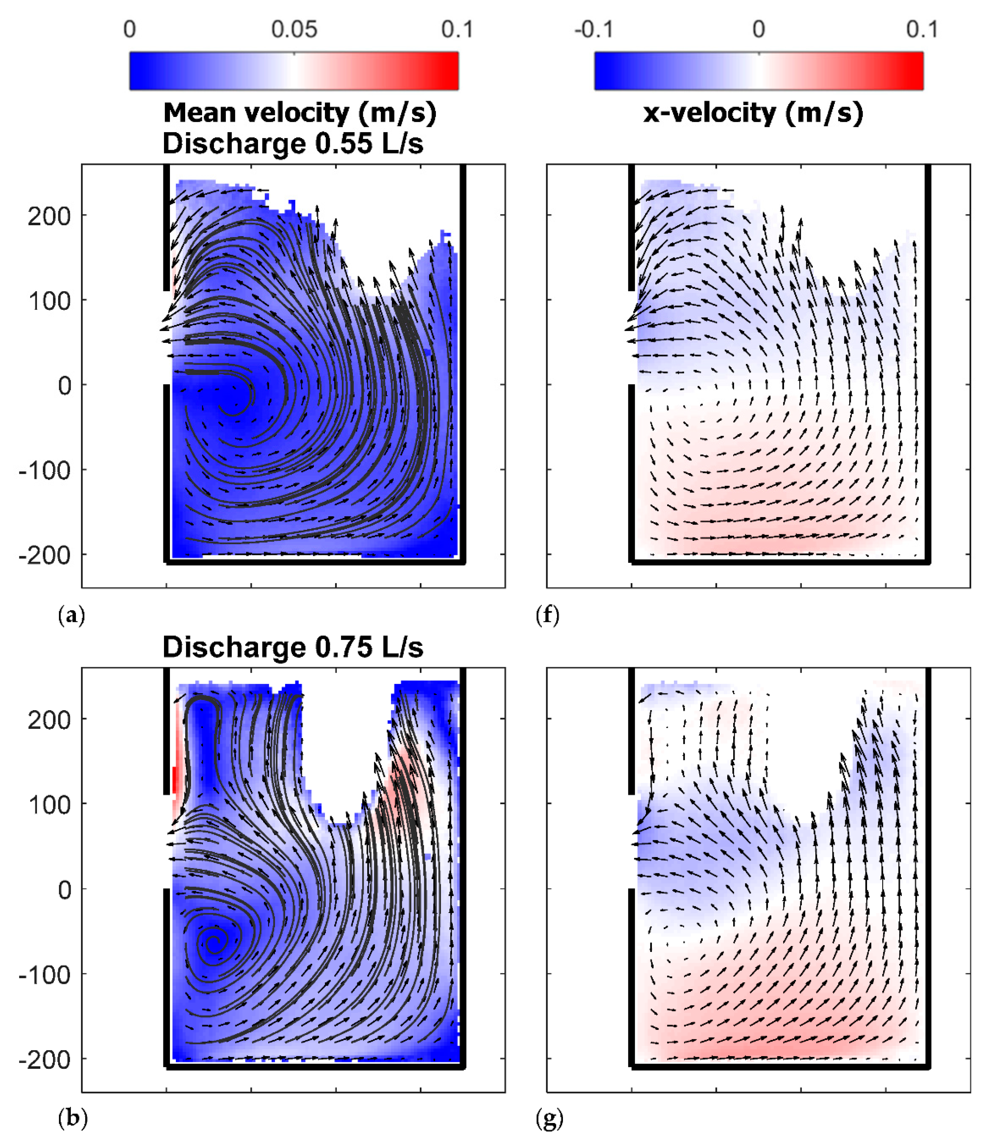
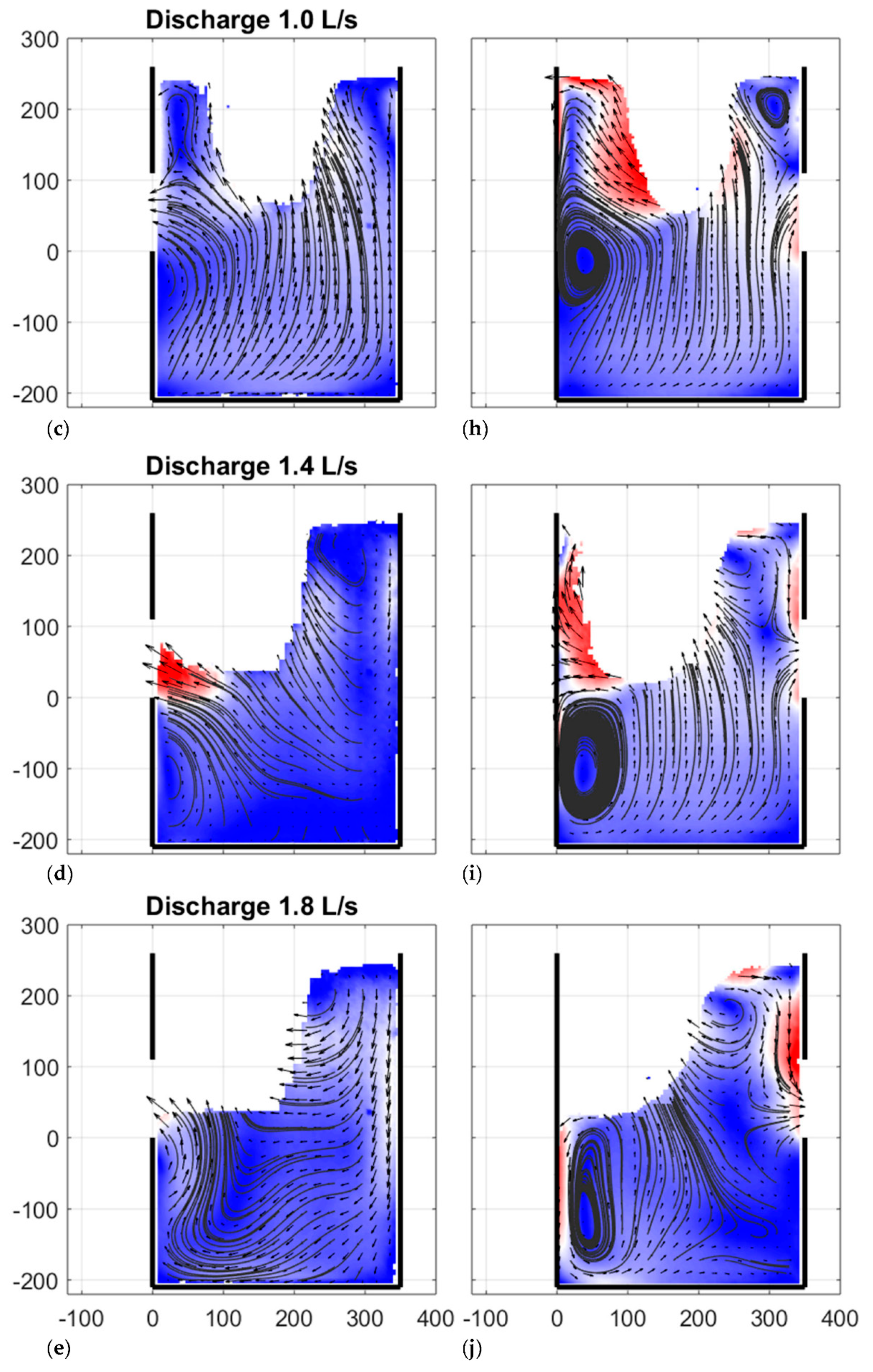
Rietveld et al. [13] showed that in the case of relatively high discharges (≥1.8 L/s) the measured efficiency (in a gully pot with the outlet at the back) is significantly smaller than the efficiency according to equation 1. Rainfall events causing these large discharges lasting at least 10 min occur ~2 times a year in The Netherlands [23]. Therefore, equation 1 can be used for most rainfall events (if the sediment bed level is not too high). Nevertheless, the influence of the discharge on the flow pattern is assessed to clarify the effect of (high) discharges. Figure 14 shows the mean velocity and x-velocity at several discharges in a gully pot with a depth of 0.21 m.
The water flows towards the outlet and the impinging jet, which together determine the flow pattern in the gully pot, in the POI. Figure 14a–e show that the impinging jets move to the left (i.e., the side of the outlet) at increased discharges. This moves the eddy, which is found below the outlet pipe, closer to the gully pot wall, until its influence on the surrounding flow becomes negligible in Figure 14e. This eddy affects the flow direction close to the gully pot bottom as can be seen in Figure 14 f–j. At discharges <1.4 L/s the flow is directed to the right, and at ~1.4 L/s the direction starts to change.
The monitored plane in Figure 14 is the vertical plane of symmetry of the gully pot. Figure 15 shows the horizontal flow field close to the gully pot bottom (plane 4 in Figure 5). The flow field at a discharge of 0.55 and 1.0 L/s is relatively symmetrical over a vertical line in the middle, while for a discharge of 1.8 L/s the flow field is asymmetrical. This asymmetry could be caused by an uneven spread of the discharge over the three impinging jets.
For the discharge of 0.55 and 1.0 L/s the in-plane velocity component is towards the bottom in Figure 15, which corresponds with towards the right in Figure 14, while at a discharge of 1.8 L/s, the flow directions change and an eddy is present.
Figure 14e–g show a smooth change in the flow pattern, while the flow velocities increase, the flow patterns are to a large extent similar. Figure 14h,j show a significant change in the flow pattern, which, at least, partially explains the observation of Rietveld et al. [13] that the efficiency strongly decreases at discharges ≥1.8 L/s.
Another important effect is short-circuiting of the impinging jet to the outlet at these high discharges (Figure 14d,e), which causes direct transport of solids to the outlet. This implies that the gully pot can no longer be regarded as a completely mixed reactor, which was assumed in the derivation of Equation (1).
3.4. The Effect of the Gully Pot Depth
Rietveld et al. [13] found that the depth of the gully pot determines at what bed level depth the accumulation rate starts to decrease, while the efficiency below or exceeding that depth is hardly influenced by the gully pot depth. Therefore, it is expected that the flow patterns are also relatively similar. Figure 16 shows the comparison between the flow fields in gully pots with different depths.
The differences in the flow pattern shown in Figure 16, can mainly be found in the eddy below the outlet. This eddy is enlarged in the case of a deeper gully pot. In some areas, the flow velocities are higher in the shallower gully pot, which can be seen from the colour differences.
3.5. The Effect of the Outlet Position
The tests of Rietveld et al. [13] with different outlet positions show that this parameter strongly influences the removal efficiency. The flow field of a gully pot with the outlet opposite to the inlet is compared with one with the outlet adjacent to the inlet in Figure 17.
For gully pots with an outlet at the front (Figure 17f–j) and discharge >0.55 L/s, the water which leaves the impinging jet is mainly directed upwards and to the back wall of the gully pot. This can effectively separate entrained solids and the outlet, which results in a larger removal efficiency than for gully pots with an outlet at the back [13]. The assumption of a completely mixed reactor for Equation (1) is violated, which explains why this equation cannot be used for this gully pot layout.
For a discharge of 0.55 L/s (Figure 17f), the flow is less strongly directed to the back wall of the gully pot. In this case, the impinging jet is close to the outlet at the front. This could cause immediate transport of entrained solids to the outlet pipe, which reduces the removal efficiency, compared with a gully pot with the outlet at the back.
4. Conclusions
Flow measurements have been performed with PIV and LDA. The two measurement techniques provide similar mean flow velocities both in direction and magnitude in areas where no air bubbles are entrained in the water. The PIV measurements are used to study the overall flow field and the LDA measurements to study the turbulent fluctuations.
The multiphase character of the flow strongly influences the flow field in a gully pot. This affects the solids deposition and should, therefore, be incorporated in studies like, e.g., Yang et al. [14] and Faram and Harwood [17] who simulated the removal efficiency in a gully pot by means of CFD. A validated CFD model could be used to assess the effect of other gully pot geometries and hydraulic conditions on the flow pattern and the removal efficiency, eventually such a model can be applied to search for a geometry that optimises the removal efficiency.
The shape of the sediment bed depends on the solids’ characteristics and the gully pot hydraulics. Regarding the hydraulics, the position of the impinging jets and the high flow velocities close to the impinging jets determine the distribution of sand in the gully pot in the initial stage. At higher bed levels, the flow velocity close to the bed increases and becomes important as well, since sediment can be transported over the bed as bed load. Finally, the accumulation rate decreases strongly in areas where both the mean flow velocity and turbulent kinetic energy (TKE) are high. In these areas, resuspension from the bed occurs.
The discharge and outlet location strongly influence the flow pattern and removal efficiency. Therefore, reducing a gully pot to a completely mixed reactor, as proposed by Butler and Karunaratne [12], is valid up to a point only. The assumption can be violated at high discharges due to effective separation of the inflow and the outflow in gully pots with the outlet at the front, and due to short-circuiting in gully pots with the outlet at the back.
The removal efficiency depends on the solids’ characteristics, the hydraulics, and the sediment bed level. In practice, only the latter two can be influenced. The hydraulics are mainly determined by the parameters discharge and outlet location. These parameters can be influenced in practice when a new urban area is designed by the choice of the number of gully pots and the type of connection of the outlet pipe. The sediment bed level can be controlled by gully pot cleaning.
Author Contributions
Conceptualisation, M.R., F.C. and J.L.; methodology, M.R. and F.C.; formal analysis, M.R. and D.d.R.; investigation, M.R. and D.d.R.; resources, M.R.; visualisation, M.R. and D.d.R.; writing—original draft preparation, M.R.; writing—review and editing, F.C. and J.L.; supervision, F.C. and J.L.; project administration, J.L.; funding acquisition, J.L. All authors have read and agreed to the published version of the manuscript.
Funding
This research was funded by the Dutch ‘Kennisprogramma Urban Drainage’ (Knowledge Programme Urban Drainage) for funding this research. The involved parties are: ARCADIS, Deltares, Evides, Gemeente Almere, Gemeente Arnhem, Gemeente Breda, Gemeente Den Haag, Gemeentewerken Rotterdam, Gemeente Utrecht, GMB Rioleringstechniek, KWR Watercycle Research Institute, Royal HaskoningDHV, Stichting RIONED, STOWA, Sweco, Tauw, vandervalk+degroot, Waterschap De Dommel, Waternet and Witteveen+Bos.
Acknowledgments
The authors thank Deltares for providing the space, and Gosse Oldenziel and Wout Bakker for the (theoretical and practical) support of the PIV and LDA measurements, respectively.
Conflicts of Interest
The authors declare no conflict of interest. The funders had no role in the design of the study; in the collection, analyses, or interpretation of data; in the writing of the manuscript, or in the decision to publish the results.
Appendix A

Table A1.
Overview of the performed PIV tests.
| Test Name | POI | Discharge (L/s) | Gully Pot Depth (m) | Outlet Position |
|---|---|---|---|---|
| F055DhalfV1 | P1 | 0.55 | 0.21 | Back |
| F075DhalfV1 | P1 | 0.75 | 0.21 | Back |
| F100DhalfV1 | P1 | 1.0 | 0.21 | Back |
| Bed1 F100DhalfV1 | P1 + bed 1 | 1.0 | 0.21 | Back |
| Bed2 F100DhalfV1 | P1 + bed 2 | 1.0 | 0.21 | Back |
| Bed3 F100DhalfV1 | P1 + bed 3 | 1.0 | 0.21 | Back |
| F140DhalfV1 | P1 | 1.4 | 0.21 | Back |
| F180DhalfV1 | P1 | 1.8 | 0.21 | Back |
| F055DfullV1 | P1 | 0.55 | 0.39 | Back |
| F075DfullV1 | P1 | 0.75 | 0.39 | Back |
| F100DfullV1 | P1 | 1.0 | 0.39 | Back |
| F140DfullV1 | P1 | 1.4 | 0.39 | Back |
| F180DfullV1 | P1 | 1.8 | 0.39 | Back |
| F055DhalfV2 | P2 | 0.55 | 0.21 | Back |
| F100DhalfV2 | P2 | 1.0 | 0.21 | Back |
| F180DhalfV2 | P2 | 1.8 | 0.21 | Back |
| F055DfullV2 | P2 | 0.55 | 0.39 | Back |
| F100DfullV2 | P2 | 1.0 | 0.39 | Back |
| F180DfullV2 | P2 | 1.8 | 0.39 | Back |
| F055DfullV3 | P3 | 0.55 | 0.39 | Back |
| F100DfullV3 | P3 | 1.0 | 0.39 | Back |
| F180DfullV3 | P3 | 1.8 | 0.39 | Back |
| F055DfullV4 | P4 | 0.55 | 0.39 | Back |
| F100DfullV4 | P4 | 1.0 | 0.39 | Back |
| F180DfullV4 | P4 | 1.8 | 0.39 | Back |
| F055DhalfV4 | P4 | 0.55 | 0.21 | Back |
| F100DhalfV4 | P4 | 1.0 | 0.21 | Back |
| F180DhalfV4 | P4 | 1.8 | 0.21 | Back |
| F055DfullV5 | P5 | 0.55 | 0.39 | Back |
| F100DfullV5 | P5 | 1.0 | 0.39 | Back |
| F180DfullV5 | P5 | 1.8 | 0.39 | Back |
| F055DhalfV5 | P5 | 0.55 | 0.21 | Back |
| F100DhalfV5 | P5 | 1.0 | 0.21 | Back |
| F180DhalfV5 | P5 | 1.8 | 0.21 | Back |
| F055DhalfV1 | P1 | 0.55 | 0.21 | Front |
| F075DhalfV1 | P1 | 0.75 | 0.21 | Front |
| F100DhalfV1 | P1 | 1.0 | 0.21 | Front |
| F140DhalfV1 | P1 | 1.4 | 0.21 | Front |
| F180DhalfV1 | P1 | 1.8 | 0.21 | Front |
| F055DfullV1 | P1 | 0.55 | 0.39 | Front |
| F075DfullV1 | P1 | 0.75 | 0.39 | Front |
| F100DfullV1 | P1 | 1.0 | 0.39 | Front |
| F140DfullV1 | P1 | 1.4 | 0.39 | Front |
| F180DfullV1 | P1 | 1.8 | 0.39 | Front |
| F055DfullV3 | P3 | 0.55 | 0.39 | Front |
| F100DfullV3 | P3 | 1.0 | 0.39 | Front |
| F180DfullV3 | P3 | 1.8 | 0.39 | Front |
| F055DfullV4 | P4 | 0.55 | 0.39 | Front |
| F100DfullV4 | P4 | 1.0 | 0.39 | Front |
| F180DfullV4 | P4 | 1.8 | 0.39 | Front |
| F055DhalfV4 | P4 | 0.55 | 0.21 | Front |
| F100DhalfV4 | P4 | 1.0 | 0.21 | Front |
| F180DhalfV4 | P4 | 1.8 | 0.21 | Front |
| F055DfullV5 | P5 | 0.55 | 0.39 | Front |
| F100DfullV5 | P5 | 1.0 | 0.39 | Front |
| F180DfullV5 | P5 | 1.8 | 0.39 | Front |
| F055DhalfV5 | P5 | 0.55 | 0.21 | Front |
| F100DhalfV5 | P5 | 1.0 | 0.21 | Front |
| F180DhalfV5 | P5 | 1.8 | 0.21 | Front |
References
- Young, R.A.; Wiersma, J.L. The role of rainfall impact in soil detachment and transport. Water Resour. Res. 1973, 9, 1629–1636. [Google Scholar] [CrossRef]
- Van Bijnen, M.; Korving, H.; Langeveld, J.G.; Clemens, F.H.L.R. Quantitative impact assessment of sewer condition on health risk. Water 2018, 10, 245. [Google Scholar] [CrossRef] [Green Version]
- Delleur, J.W. New results and research needs on sediment movement in urban drainage. Water Resour. Plan. Manag. 2001, 127, 186–193. [Google Scholar] [CrossRef]
- Chebbo, G.; Bachoc, A. Characterization of suspended solids in urban wet weather discharges. Water Sci. Technol. 1992, 25, 171–179. [Google Scholar] [CrossRef]
- Fulcher, G.A. Urban stormwater quality from a residential catchment. Sci. Total Environ. 1994, 146–147, 535–542. [Google Scholar] [CrossRef]
- Gromaire, M.C.; Garnaud, S.; Saad, M.; Chebbo, G. Contribution of different sources to the pollution of wet weather flows in combined sewers. Water Res. 2001, 35, 521–533. [Google Scholar] [CrossRef]
- Post, J.A.B.; Pothof, I.W.M.; Dirksen, J.; Baars, E.J.; Langeveld, J.G.; Clemens, F.H.L.R. Monitoring and statistical modelling of sedimentation in gully pots. Water Res. 2016, 88, 245–256. [Google Scholar] [CrossRef] [PubMed] [Green Version]
- De Man, H.; Van den Berg, H.H.J.L.; Leenen, E.J.T.M.; Schijven, J.F.; Schets, F.M.; Van der Vliet, J.C.; Van Knapen, F.; De Roda Husman, A.M. Quantitative assessment of infection risk from exposure to waterborne pathogens in urban floodwater. Water Res. 2014, 48, 90–99. [Google Scholar] [CrossRef]
- Ten Veldhuis, J.A.E.; Clemens, F.H.L.R. The efficiency of asset management strategies to reduce urban flood risk. Water Sci. Technol. 2011, 64, 1317–1324. [Google Scholar] [CrossRef]
- Chen, Y.; Cowling, P.; Polack, F.; Remde, S.; Mourdjis, P. Dynamic optimisation of preventative and corrective maintenance schedules for a large scale urban drainage system. Eur. J. Oper. Res. 2017, 257, 494–510. [Google Scholar] [CrossRef]
- Rietveld, M.W.J.; Clemens, F.H.L.R.; Langeveld, J.G. Monitoring and statistical modelling of the solids accumulation rate in gully pots. Urban Water J. 2020, 17, 549–559. [Google Scholar] [CrossRef]
- Butler, D.; Karunaratne, S.H.P.G. The suspended solids trap efficiency of the roadside gully pot. Water Res. 1995, 29, 719–729. [Google Scholar] [CrossRef]
- Rietveld, M.W.J.; Clemens, F.H.L.R.; Langeveld, J.G. Solids dynamics in gully pots. Urban Water J. 2020, 17, 669–680. [Google Scholar] [CrossRef]
- Yang, H.; Zhu, D.Z.; Li, L. Numerical modeling on sediment capture in catch basins. Water Sci. Technol. 2018, 77, 1346–1354. [Google Scholar] [CrossRef]
- Tang, Y.; Zhu, D.Z.; Rajaratnam, N.; Van Duin, B. Experimental study of hydraulics and sediment capture efficiency in catchbasins. Water Sci. Technol. 2016, 74, 2717–2726. [Google Scholar] [CrossRef]
- Howard, A.K.; Mohseni, O.; Gulliver, J.S.; Stefan, H.G. Hydraulic analysis of suspended sediment removal from storm water in a standard sump. J. Hydraul. Eng. 2012, 138, 491–502. [Google Scholar] [CrossRef]
- Faram, M.; Harwood, R. A method for the numerical assessment of sediment interceptors. Water Sci. Technol. 2003, 47, 167–174. [Google Scholar] [CrossRef]
- Westerweel, J.; Elsinga, G.E.; Adrian, R.J. Particle image velocimetry for complex and turbulent flows. Annu. Rev. Fluid Mech. 2013, 45, 409–436. [Google Scholar] [CrossRef]
- Drain, L.E. The Laser Doppler Techniques; Wiley-Interscience: Chichester, UK, 1980. [Google Scholar]
- Westerweel, J.; Scarano, F. Universal outlier detection for PIV data. Exp. Fluids 2005, 39, 1096–1100. [Google Scholar] [CrossRef]
- Nieuwstadt, F.T.M.; Westerweel, J.; Boersma, B.J. Turbulence: Introduction to Theory and Application of Turbulent Flows; Springer: Cham, Switzerland, 2016. [Google Scholar]
- Wilczek, M.; Narita, Y. Wave-number-frequency spectrum for turbulence from a random sweeping hypothesis with mean flow. Phys. Rev. E 2012, 86, 066308. [Google Scholar] [CrossRef] [PubMed] [Green Version]
- Beersma, J.; Versteeg, R. Basisstatistiek Voor Extreme Neerslag in Nederland; STOWA: Amersfoort, The Nederland, 2019. [Google Scholar]
- Heikkila, J.; Olli, S. A four-step camera calibration procedure with implicit image correction. In Proceedings of the IEEE Computer Society Conference on Computer Vision and Pattern Recognition, San Juan, Puerto Rico, 17–19 June 1997; IEEE: New York, NY, USA, 1997; pp. 1106–1112. [Google Scholar]
- Zhang, Z. A flexible new technique for camera calibration. IEEE Trans. Pattern Anal. Mach. Intell. 2000, 22, 1330–1334. [Google Scholar] [CrossRef] [Green Version]
- Avila, H.; Pitt, R.; Durrans, S.R. Factors affecting scour of previously captured sediment from stormwater catchbasin sumps. J. Water Manag. Model. 2008. [Google Scholar] [CrossRef]
- Terfous, A.; Hazzab, A.; Ghenaim, A. Predicting the drag coefficient and settling velocity of spherical particles. Powder Technol. 2013, 239, 12–20. [Google Scholar] [CrossRef]
- Avila, H.; Pitt, R.; Clark, S.E. Development of effluent concentration models for sediment scoured from catchbasin sumps. J. Irrig. Drain E. 2011, 137, 114–120. [Google Scholar] [CrossRef]
Figure 1.
Roadside gully pot.

Figure 2.
Experimental setup and camera positions 1. Aluminium canal 2. Gully pot 3. Control valve. 4. Water reservoir with pump 5. Hose with valve and flow meter. (a) Setup with the outlet at the back; (b) Setup with the outlet at the front.
Figure 2.
Experimental setup and camera positions 1. Aluminium canal 2. Gully pot 3. Control valve. 4. Water reservoir with pump 5. Hose with valve and flow meter. (a) Setup with the outlet at the back; (b) Setup with the outlet at the front.

Figure 3.
Camera setup for Stereo Particle Image Velocimetry (SPIV). 1. Camera equipped with Scheimpflug adapter 2. Acrylate prism 3. Plane of Interest (POI). (a) Photo of the setup; (b) Schematic drawing of the setup.
Figure 3.
Camera setup for Stereo Particle Image Velocimetry (SPIV). 1. Camera equipped with Scheimpflug adapter 2. Acrylate prism 3. Plane of Interest (POI). (a) Photo of the setup; (b) Schematic drawing of the setup.

Figure 4.
Laser Doppler Anemometry (LDA) setup. 1. Optical receiver 2. Laser 3. Laser beam (a) Photo of the setup; (b) Schematic drawing of the setup.
Figure 4.
Laser Doppler Anemometry (LDA) setup. 1. Optical receiver 2. Laser 3. Laser beam (a) Photo of the setup; (b) Schematic drawing of the setup.

Figure 5.
Side and front view of the planes of interest (in red) in the gully pot. The blue line indicates the water level, the grey line the second bottom.
Figure 5.
Side and front view of the planes of interest (in red) in the gully pot. The blue line indicates the water level, the grey line the second bottom.

Figure 6.
(a) The build-up of the sediment bed was carefully stopped, while the water level was kept constant and consecutively stereo photos of the bed were made with the shown setup. 1. Cameras 2. Light source 3. Sediment bed; (b) The printed sediment bed which is covered with a glued layer of sand.

Figure 7.
(a) Image used to calibrate the stereo photography setup; (b) Image of the sediment bed used to create the artificial sediment bed shown in Figure 6b.
Figure 7.
(a) Image used to calibrate the stereo photography setup; (b) Image of the sediment bed used to create the artificial sediment bed shown in Figure 6b.

Figure 8.
The retained mass and efficiency at which the stereo photos were obtained and the corresponding 3D representation of the sediment beds. The figures of the sediment bed also show the gully pot bottom and back wall including the outlet.
Figure 8.
The retained mass and efficiency at which the stereo photos were obtained and the corresponding 3D representation of the sediment beds. The figures of the sediment bed also show the gully pot bottom and back wall including the outlet.

Figure 9.
(a) Streamlines and mean velocity for the test with sand trap depth of 0.39 m, outlet at the back, and discharge 1.0 L/s. The white area in the upper part of the figure represents an area with a high fraction of air bubbles (entrained by the impinging waterjet) which disturbed the PIV measurements; (b) The POI and gully pot layout of the test.

Figure 10.
PIV and LDA results for the test with a sand trap depth of 0.21 m, outlet at the back, and discharge 1.0 L/s. (a,b) Comparisons of the mean flow velocity; (c) The difference scalar as defined by equation 18; (d,e) TKE and TI based upon the LDA measurements.
Figure 10.
PIV and LDA results for the test with a sand trap depth of 0.21 m, outlet at the back, and discharge 1.0 L/s. (a,b) Comparisons of the mean flow velocity; (c) The difference scalar as defined by equation 18; (d,e) TKE and TI based upon the LDA measurements.


Figure 11.
Power spectrum of the two velocity components of the top left measurement point in Figure 10b,c. The spectrum contains the expected power −5/3 dependency on the frequency. The cut-off frequency originates from the analogue filter used in the measurement setup to cancel out high-frequency noise.

Figure 12.
The effect of a growing sediment bed on the flow field. The sand traps in the figures are filled with sediment (a) 0% filled; (b) 24% filled; (c) 62% filled; (d) 91% filled.
Figure 12.
The effect of a growing sediment bed on the flow field. The sand traps in the figures are filled with sediment (a) 0% filled; (b) 24% filled; (c) 62% filled; (d) 91% filled.

Figure 13.
The effect of a growing sediment bed on (a–c) the mean velocity, and (d–f) the turbulent kinetic energy (TKE) (of which the latter is measured at 7 mm from to the sediment bed).
Figure 13.
The effect of a growing sediment bed on (a–c) the mean velocity, and (d–f) the turbulent kinetic energy (TKE) (of which the latter is measured at 7 mm from to the sediment bed).

Figure 14.
The effect of the discharge on the flow field. (a–e) Mean velocity; (f–j) x-velocity.


Figure 15.
Flow field 3 cm above the gully pot bottom. The outlet is located at the top and the inlet at the bottom of the figures. The arrows indicate the in-plane flow direction and the colour scheme the out of plane component (blue towards the bottom and red towards the water surface). (a) Discharge 0.55 L/s; (b) Discharge 1.0 L/s; (c) Discharge 1.8 L/s.

Figure 16.
The effect of the gully pot depth on the flow field at several discharges. (a–c) Gully pot with depth 0.21 m; (d–f) Gully pot with depth 0.39 m.
Figure 16.
The effect of the gully pot depth on the flow field at several discharges. (a–c) Gully pot with depth 0.21 m; (d–f) Gully pot with depth 0.39 m.

Figure 17.
The effect of the outlet position on the flow field at several discharges. (a–e) Gully pot with outlet at the back; (f–j) Gully pot with outlet at the front.
Figure 17.
The effect of the outlet position on the flow field at several discharges. (a–e) Gully pot with outlet at the back; (f–j) Gully pot with outlet at the front.


Publisher’s Note: MDPI stays neutral with regard to jurisdictional claims in published maps and institutional affiliations. |
© 2020 by the authors. Licensee MDPI, Basel, Switzerland. This article is an open access article distributed under the terms and conditions of the Creative Commons Attribution (CC BY) license (http://creativecommons.org/licenses/by/4.0/).
Share and Cite
MDPI and ACS Style
Rietveld, M.; de Rijke, D.; Langeveld, J.; Clemens, F. Sediment Morphology and the Flow Velocity Field in a Gully Pot: An Experimental Study. Water 2020, 12, 2937. https://doi.org/10.3390/w12102937
AMA Style
Rietveld M, de Rijke D, Langeveld J, Clemens F. Sediment Morphology and the Flow Velocity Field in a Gully Pot: An Experimental Study. Water. 2020; 12(10):2937. https://doi.org/10.3390/w12102937
Chicago/Turabian StyleRietveld, Matthijs, Demi de Rijke, Jeroen Langeveld, and Francois Clemens. 2020. "Sediment Morphology and the Flow Velocity Field in a Gully Pot: An Experimental Study" Water 12, no. 10: 2937. https://doi.org/10.3390/w12102937
Note that from the first issue of 2016, this journal uses article numbers instead of page numbers. See further details here.