Developing a Reliability Index of Low Impact Development for Urban Areas

Abstract

A defining characteristic of the urbanization is the transformation of existing pervious areas into impervious areas during development. This leads to numerous hydrologic and environmental problems such as an increase in surface runoff due to excess rainfall, flooding, the deterioration of water quality, and an increase in nonpoint source pollution. Several studies propose supplementary measures on environmental change problems in development areas using the low impact development technique. This study investigated the reduction of nonpoint source pollutant loads and flooding in catchments through urban catchment rainfall–runoff management. For the quantitative assessment of flood disasters and water pollution problems, we propose a reliability evaluation technique. This technique refers to a series of analysis methods that determine the disaster prevention performance of the existing systems. As the two factors involve physical quantities of different dimensions, a reliability evaluation technique was developed using the distance measure method. Using the storm water management model, multiple scenarios based on synthetic rainfall in the catchment of the Daerim 2 rainwater pumping station in Seoul, South Korea, were examined. Our results indicate the need for efficient management of natural disaster risks that may occur in urban catchments. Moreover, this study can be used as a primary reference for setting a significant reduction target and facilitating accurate decision making concerning urban drainage system management.

1. Introduction

Climate change and rapid urbanization aggravate natural disasters such as flooding by increasing the water quantity and the amount of pollutants discharged from nonpoint sources during rainfall. In 2014, the Intergovernmental Panel on Climate Change (IPCC) reported that the increasing impact of climate change, caused by human activities and industrial development, is undeniable [1]. A typical climate change phenomenon includes changes in the frequency, intensity, duration, and timing of weather and climate extremes, and can result in unprecedented extreme rainfall events. The frequent occurrence of extreme rainfall events incurs human casualties and economic losses by devastating natural disasters such as floods and landslides [2]. In particular, the interest in studying urban disasters is rising as the property values increase because of continuous population growth, overpopulation, and regional development [3,4]. Rapid and continuous migration from rural areas to more densely inhabited cities increases urban sprawl and increases the susceptibility of a greater portion of the population to the risks of natural disasters [5]. Moreover, the inflow of various pollutants from industrialization is increasing, and consequently, water pollution in urban areas is rapidly aggravating [6]. Therefore, pollutants are washed out into catchment areas during excessive rainfall and severe flood events [2]. In urban catchments, high concentrations of pollutants are discharged in the early stages of rainfall and rapidly decrease as rainfall continues. This phenomenon, referred to as the first flush, occurs universally. It is necessary to determine the pollutant load per subcatchment to analyze the environmental impact of these flushed pollutants on the surrounding basin.

Among nonpoint source pollutants generated from various land uses, paved areas such as roads and bridges typically have higher ratios of impervious surface coverage than other land-use types. Impervious surfaces experience more surface runoff during rainfall. Moreover, these structures also show very rapid changes in runoff quantity and water quality concentration. Therefore, a water cycle analysis considering urban water quantity and water quality needs be conducted simultaneously from a comprehensive perspective. Furthermore, accurate research is required to promote rational decision making for natural disaster prevention.

The term low impact development (LID) refers to the systems and practices that use or mimic natural processes that result in the infiltration, evapotranspiration, or use of stormwater to reduce flood impacts and improve water quality in urban areas. The LID’s design technique minimizes rainfall–runoff occurring in the impermeable layers and facilitates restoration closest to the natural hydrological state before development [7,8,9]. In addition, the United States Environmental Protection Agency (US EPA) defines LID as a planning and design approach for overcoming the problems caused by the changing hydrologic properties from urbanization, which preserves the hydrologic function in the region. [10]. LID’s concept is drawing attention as a new paradigm of urban water management for the efficient handling of urban water hazards. Moreover, studies are being conducted on the practical application of LID systems and their implications [11,12,13].

In the 2000s, when LID technology’s interest started to increase, separate rainwater management was necessary by reducing the impervious area, and restoring the catchment to its natural state was proposed [14]. Several studies were conducted to design a LID facility that could be applied in the housing site development process. These studies are conducted to establish the basis for sustainable development through the development of facilities capable of reducing runoff in catchments [15,16]. In the United States, research has been conducted to establish a standard manual for constructing and maintaining LID facilities. Standard deductions shared between these studies included the use of field-based knowledge for addressing potential problems, whereby regional characteristics are modeled and provide data for decision making [17,18,19].

Field-based studies categorize LID systems into infiltration- and storage-type facilities and have evaluated the water cycle effect and the ability of these systems to reduce nonpoint sources [20,21,22]. Moreover, previous studies have established the flood control capability and nonpoint source reduction effect by element facilities such as permeable pavements [23,24], green roofs [25], vegetation-type facilities [26], and fine-media stormwater filtration systems [27]. Furthermore, according to the size of catchment areas, LID systems’ performance has also been determined [28,29].

Continual research is conducted to reduce flood runoff and improve water quality management, considering extreme weather events such as climate change. In particular, the interest in technological development to enhance water management energy efficiency, particularly in primary developed countries, is rising [11,12,13].

For disaster prevention in urban catchments, developed countries such as the United States and the European Union have prescribed strict management via optimum means such as quantitative risk assessment. It has been emphasized that disaster prevention outcomes vary greatly depending on the quantitative risk assessment [30,31]. However, relatively few studies have focused on the design and risk assessment of urban nonpoint source pollution reduction facilities considering flood disaster and water pollution. In particular, concerning a quantitative effect analysis of the LID technique, various analysis methods are in mixed-use, and research that facilitates result-based transparent decision making is required.

In reliability analysis, all engineering systems, including hydrological systems, have a certain probability of failure in fulfilling their intended purpose. For example, in a flood control system, the control of all extreme flood cases is not possible. For urban drainage systems, the utilization of full functionalities depends on the circumstances. Reliability problems of engineering systems are mainly analyzed based on the relationship between supply and demand. A safety level has been adopted for marginal designs and an estimate for similar facilities in the past. However, with these approaches, quantitative analysis is not possible, and it is also difficult to consider each factor [32].

Studies were conducted to analyze the reliability and economic impact of the water utility service to determine the supply priority in the water supply issue in a drought [33,34]. The studies on regional drought analysis were also carried out by estimating the groundwater level threshold through time-series probability analysis of the observed groundwater-level data [35,36]. In addition, research has been conducted on the reliability analysis of future water supply for multipurpose dams [37].

Studies approaching the flood control function of the sewer network based on the reliability theory have been conducted to evaluate the flood control performance in connection with the fuzzy theory or estimating the reliability index by analyzing the uncertainties in parameters directly affecting the runoff [38,39]. Lee [40] and Lee and Park [41] developed a reliability estimation method for various excess rainfall scenarios by presenting a sewer network reliability evaluation method based on the flood volume and number of overflow occurrence points. Furthermore, Lee and Kim [42] proposed a reliability-based multi-dimensional flood damage analysis method considering the amount of flood damage in urban drainage systems’ reliability calculation process.

In urban areas, the proportion of impermeable pavement is high, and thus the peak flood quantity and transfer time of nonpoint sources are also high. Therefore, urban water management schemes should assess both water quantity and water quality aspects. As each factor mentioned is a physical quantity with a different dimension, a specific methodological solution is required for a comprehensive investigation. In this study, a reliability analysis based on the reliability evaluation method proposed by Lee and Kim [42] was conducted to address this issue. Furthermore, we propose that the difference in the risk of disasters within a system designed under the same design frequency can be quantitatively analyzed. The analysis determines how stable performance outcomes are obtained for the configured sewer network system in disaster prevention against flood disasters and water pollution problems.

This study aims to propose a reliability-based evaluation technique that allows the designers to quantitatively evaluate the effect of runoff reduction facilities, including the LID technique, on flood-runoff reduction, and water quality management. The reliability of the sewer network system is calculated from the probability of failure of expected performance, as in general structures. Usually, reliability is calculated from the probability of failure through uncertainty analysis based on a review of the variability of parameters. However, in the uncertainty analysis, only the probability of failure according to the mathematical logic in the design was considered, but the phenomena due to failure were not considered and evaluated. This study dealt with a methodology for scenario-based decision making for a design or a judgment for a quantitative evaluation of the phenomenon through simulation of the current performance of the system in calculating the reliability of the sewer network system.

2. Methodologies

2.1. Overview

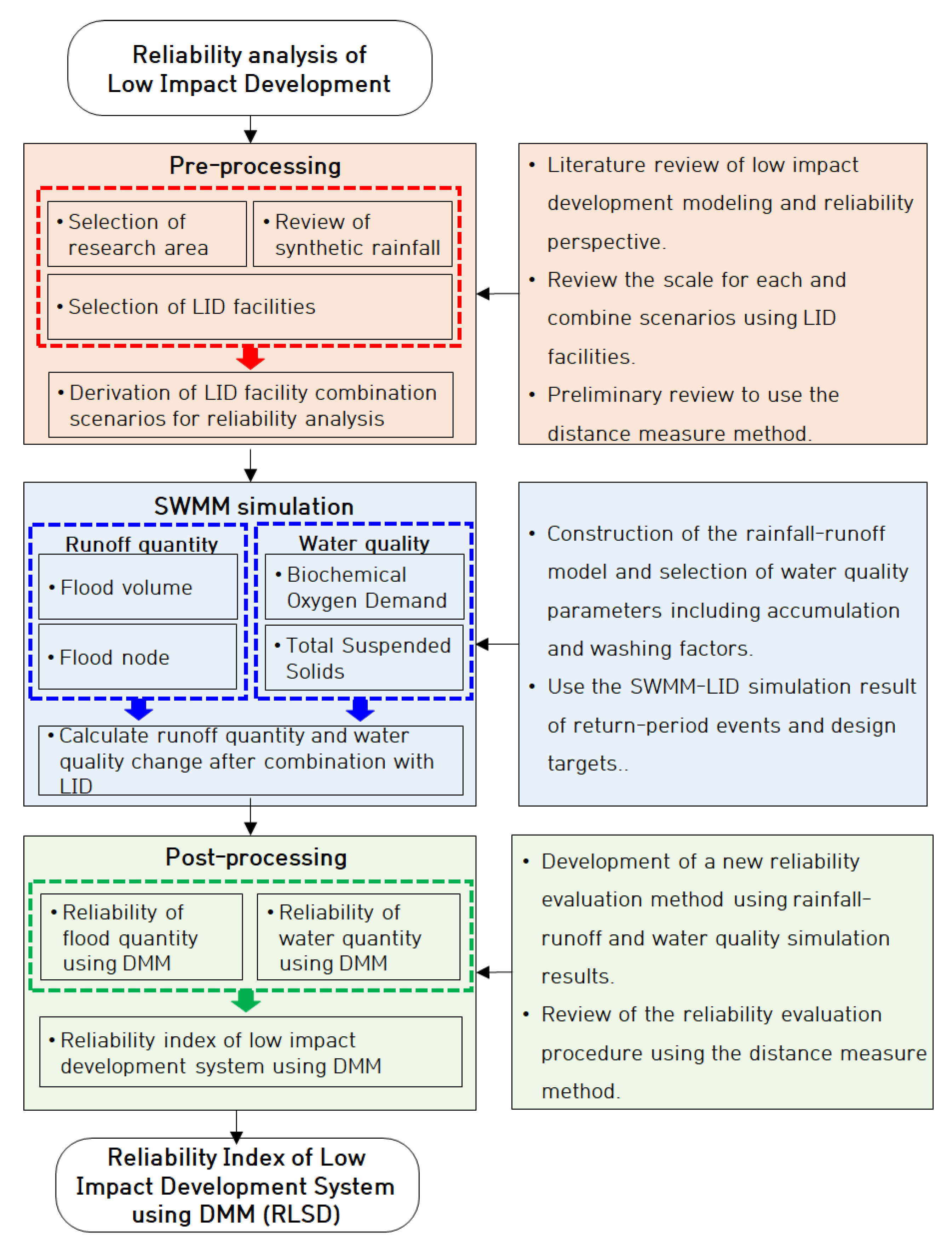
This study consists of three main parts. First, we describe the process of simulating water quantity and water quality in urban LID facilities. The development of the rainfall–runoff model and water quality parameters, including accumulation and washing factors, are also described. The storm water management model (SWMM) was used for the simulation [43,44,45]. SWMM model allows continuous simulation using synthetic and historical rainfall series. In this study, SWMM was applied to short-term rainfall modeling of selected urban areas. In addition, a description of the parameters of the LID facilities to be considered is also provided. Second, we describe the reliability evaluation method using water quantity and water quality simulation results. Various inputs and parameter values necessary for the analytical process (the construction of rainfall database, accumulation and washing parameters, a reflection of LID facilities, and change in impermeability) are also described. Subsequently, we develop a scenario for reflecting LID facilities and conduct a reliability evaluation with the analytical results of the total runoff quantity, flood volume, biochemical oxygen demand (BOD), and total suspended solids (TSS) load. Third, the new reliability evaluation technique is applied to a catchment in Daerim 2-dong, Seoul, South Korea, and the utilization plan for these results is described. Figure 1 provides the flowchart of our research methodology.

2.2. Generation of Synthetic Rainfall Data

Synthetic rainfall at a 30-, 50-, 70-, 80-, and 100-year frequency was simulated for 30 and 60 min to obtain accurate rainfall data. These data, obtained from the Seoul weather station, were used as the input data (

Table 1. Synthetic Rainfall (mm) according to Duration and Frequency obtained from a Seoul weather station (108) [50].

	Frequency	30 Years	50 Years	70 Years	80 Years	100 Years
Duration
30 min		55.2	58.8	61.1	61.8	63.4
60 min		85.7	91.5	95.2	96.6	99.0

). In the case of the Seoul weather station, it is the synthetic rainfall generated using observation data for 56 years from 1961 to 2017. The urban drainage system’s maximum design frequency was set to 30 years based on the rainwater pumping station [46]. This period is standard in Korea and allows for the smooth discharge of stormwater into rivers. In addition, a design frequency of approximately 100 years was applied to the flood protection plan of tributary streams a frequency is an estimate of how long it will be between rainfall events of a given magnitude. It is interpreted as the same concept as the return period. Taking the figures in Table 1 as an example, the return period for a 60 min rainfall total of 85.7 mm in Seoul weather station is 30 years. Therefore, in this study, considering the minimum design standard of the rainwater pumping station and the drainage basin, synthetic rainfall with a frequency of 30 to 100 years was used. For the rainfall data applied in this study, the stormwater sewer’s design frequency was exceeded and inundation occurred depending on the catchment properties. The second quartile of the Huff method was used for the synthetic rainfall distribution [47], following the method proposed by the Ministry of Land, Transport, and Maritime Affairs (2011) [48]. The reason for using the second quartile is that in the estimation of flood quantity, if effective rainfall calculation method is used, much of the peak of the synthetic rainfall hyetograph is treated as a loss due to the initial loss impact in the initial first and second quartiles, so the flood quantity may be estimated to be relatively small [49].

2.3. Low Impact Development (LID) Scenarios

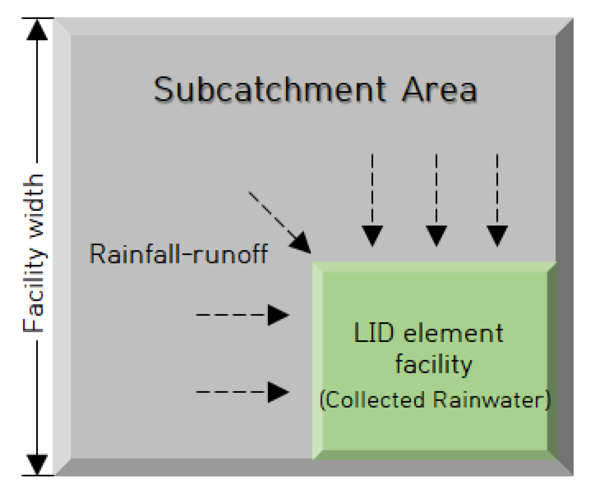
Although the approaches for implementing the water cycle to urban development vary by country, they all have the shared concept of separate rainwater management within catchments [18]. As shown in Figure 2, in separate rainwater management, rainwater discharged to rivers is minimized, and water quality and water quality are determined simultaneously. The LID module of SWMM 5.1 consists of six layers. It is based on characteristics per configuration-unit area, allowing the LID element facilities of the same specification to be applied to other subcatchments with different land cover characteristics. Simultaneously, it is possible to investigate the level of storage and circulation within each layer while maintaining the water budget balance [50]. However, depending on the type of each facility, there is a difference in the stormwater runoff storage effect because of the LID element facility.

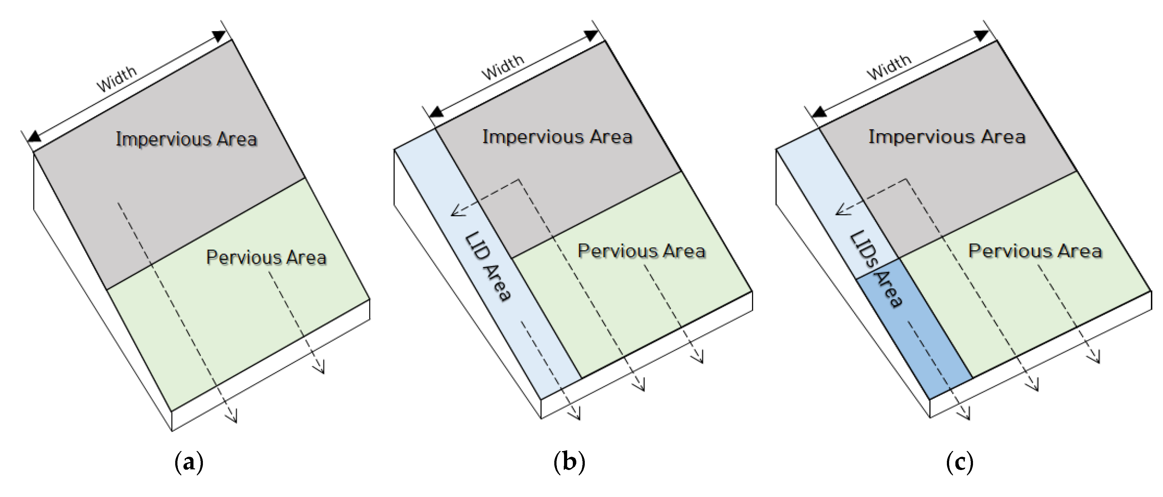
The characteristics of the subcatchments in the SWMM model are shown in Figure 3a. However, when a LID element facility is applied using the LID module, multiple LID element facilities can be applied to a single subcatchment (Figure 3b,c). When one LID element facility is applied to a single subcatchment, the stormwater runoff generated in the impervious area is transported to the LID element facility and pervious area to store and infiltrate the rainfall–runoff. The application of one LID element facility to a single subcatchment is configured according to Type A (Figure 3b). Type B represents multiple LID element facilities’ configuration to a single subcatchment (Figure 3c). Stormwater runoff treatment is simultaneously conducted in all the applied LID element facilities.

The application of LID element facilities to a single subcatchment decreases the impervious area. Therefore, the impervious area ratio must be altered accordingly. In this study, various scenarios were considered by varying the impervious area ratio of the subcatchment using the values of the area used by LID facilities (A_LID), the total area of subcatchment (A_Sub), and the impervious area ratio (P_IA) (Equation (1)). Herein, Change impervious refers to the change in the impervious area ratio with the installation of LID facilities in the existing subcatchment. LID Area is the size of the area occupied by the LID facilities, and subcatchment Area corresponds to the subcatchment area where the LID facilities are installed. Percent of impervious area (P_IA) corresponds to the impervious area’s ratio where runoff quantities cannot be permeated. Equation (1) was used to calculate the percentage of impervious area considering LID facilities in the subcatchment.

$$\mathrm{Change}\mathrm{impervious}(\%)=\frac{\left(1-\frac{A_{LID}}{A_{Sub}}\right)\times P_{IA}}{\left(100-\frac{A_{LID}}{A_{Sub}}\times P_{IA}\right)}\times 100$$

(1)

The factors affecting LID element facilities’ performance, such as infiltration and storage, were selected as the primary parameters. In this study, the following three LID facilities were considered: permeable pavements, green roofs, and infiltration trenches. For the main parameters of permeable pavements, 16 input parameter values were required, including surface layer, pavement layer, storage layer, and underdrain layer. A total of 14 input parameter values were selected for green roofs and include a surface layer, soil layer, and drainage mat. An infiltration trench required 11 input parameter values, including the surface layer, storage layer, and underdrain layer. This study’s parameters were selected based on the values proposed by Holzbauer-Schweitzer [51] (

Table 2. Summary of LID Facilities and Associated Model Parameters [51].

Layer	Parameter	Unit	Permeable Pavement	Green Roof	Infiltration Trench
Surface	Berm Height	mm	25.0	25.0	0.0
	Vegetation Volume Fraction	-	0.0	0.0	0.0
	Surface Roughness	-	0.0	0.0	0.2
	Surface Slope	percent	1.0	0.0	0.4
Soil	Thickness	mm	0.0	150.0	-
	Porosity	-	0.5	0.6	-
	Field Capacity	-	0.2	0.3	-
	Wilting Point	-	0.1	0.0	-
	Conductivity	mm/h	0.5	64.0	-
	Conductivity Slope	-	10.0	5.0	-
	Suction Head	mm	3.5	75.0	-
Storage	Thickness	mm	300.0	25.0	36.0
	Void Ratio	-	0.7	0.7	0.4
	Seepage Rate	mm/h	1.0	0.0	0.2
Pavement	Thickness	mm	150.0	-	-
	Void Ratio	-	0.2	-	-
	Impervious Surface Fraction	-	0.0	-	-
	Permeability	mm/h	500.0	-	-
Underdrain	Flow Coefficient	-	0.3	50.0	0.0
	Flow Exponent	-	0.5	0.5	0.5
	Offset Height	mm	100.0	0.0	0.0
Drainage Mat	Thickness	mm	-	1.0	-
	Void Fraction	-	-	0.5	-

).

2.4. Simulation of Water Quality Using SWMM

The measurement of BOD is commonly used to determine the contamination status of sewage by organic materials. High levels of BOD in sewage correspond to high concentrations of organic materials. Sustained high concentrations of organic materials in sewage cause anaerobic decomposition in sewer pipes and ultimately deteriorate treatment functions. Moreover, in urban areas, the increased volume of sediments, such as TSS, deposited in the sewer during rainfall leads to a temporary increase in BOD. Therefore, the TSS concentration is directly related to BOD for various pollutant particles [52]. In this regard, the National Institute of Environment Research (NIER) established BOD and SS as the most important water quality indicators that require strict monitoring for the management of sewer systems [53,54]. The Korea Environment Corporation established sewer system monitoring and modeling guidelines during rainfall, which include essential parameters such as rainfall, flow rate in sewer pipes, BOD, and TSS [55].

This study implemented the reduction target load ratio for urban nonpoint sources specified by the NIER [53,54]. We selected the subcatchment with the maximum increased load reduction rate for each combination of LID facilities for analysis. For the test and correction of the SWMM model, measurement data for runoff quantity and pollutant outflow according to rainfall events for each target catchment were required. However, in the case of the target catchment selected in this study, no measurement data on runoff quantity and pollutant outflow could be obtained for individual rainfall events. Therefore, it was necessary to test and correct the water quality model parameters, which are essential for obtaining reliable results. We obtained rainfall data in the ungauged areas from studies conducted by Yeon et al. and Yeon and used the results of the Soil Moisture Index (SMI) to estimate surface runoff [56,57]. Prior studies categorized land-use conditions as “transportation and residential areas,” and the generated pollutant loads were estimated using the average basic unit per nonpoint source as presented by NIER [53,54]. The event mean concentration (EMC) value was estimated to ensure that the value of the pollutant concentration model was close to the value of the previous results through trial-and-error parameter estimation.

Table 3. Summary estimation result of SWMM water quality model parameters for target area [57].

No.	Parameter	Unit	Residential Area
1	BOD	Max.Buildup (kg/km2)	3.14
		Rate Constant (1/day)	0.32
2	TSS	Max.Buildup (kg/km2)	27.08
		Rate Constant (1/day)	0.28

outlines the BOD and TSS load parameters applied in this study.

2.5. Distance Measure Method

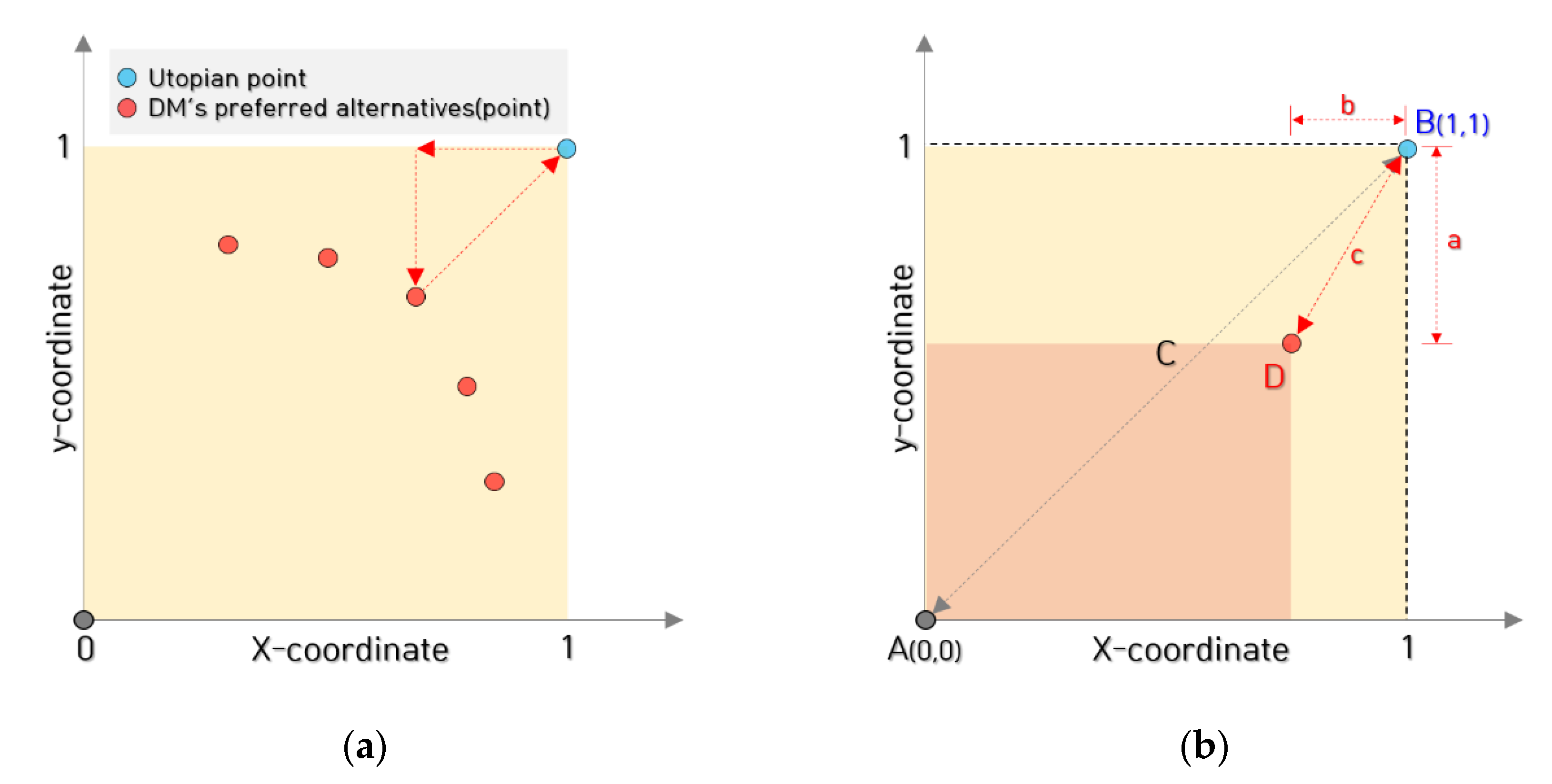
The sewer network system’s primary function is to control the performance at each frequency used in the design process. Flood control performance generally refers to the act or technique of controlling the runoff through the sewer network system to minimize flood risk. A frequency is an estimate of how long it will be between rainfall events of a given magnitude. It is interpreted as the same concept as the return period. Taking the figures in Table 1 as an example, the return period for a 60 min rainfall total of 85.7 mm in Seoul weather station is 30 years. As the importance of flood control performance due to frequent heavy rainfalls from climate change continues to be emphasized, related technological developments need to reflect the temporal and economic aspects to ensure effective flood control. This study used the distance measure method (DMM) to determine the flood control performance and pollutant reduction ability of the applied LID technology in the sewer network system. This method considers the probability of performance failure for the occurrence of rainfall events that exceed the current capacity. We applied the Utopian distance measure method to compare the dimension of the units and measure of the range of the indices considered. The Utopian approach uses the distance between the Utopian point and the current state where failure occurs. This approach is represented in Figure 4 and Equation (2).

$$\mathrm{Euclidean}\mathrm{distance}:\mathrm{c}=\sqrt{a^2+b^2}$$

(2)

The Utopian approach method in Figure 4a indicates the process of examining the reliability relationship for different analytical results. It represents the process of recognizing the ranking of alternatives given through decision making as a value and selecting the final agreed plan using the indexing concept. At this time, the distance to the utopian point is compared using Equation (2), and an alternative with the shortest distance is adopted as the agreed plan of the group. Therefore, the location of a point in the Euclidean space in Figure 4b indicates a Euclidean vector. In Figure 4b, A(0, 0) and B(1, 1) represent the distance from A, the origin of space, to the endpoint B (utopian point) as a Euclidean vector C. As shown in Figure 4b, for the water quantity and water quality parameters, values were mapped based on the maximum value “1”. The distance D from “1” was estimated using a and b in the spatial coordinates. The longer the calculated Euclidean distance, the larger the scale of damage and the risk per type of water quantity and water quality. Conversely, a closer distance to “1” represents less risk. The Utopian Approach is a suitable approach when it is difficult to synthesize the opinions of decision makers because their preferences are not concentrated in any one area but are widely distributed. This is a method of comparing the distance between decision maker’s preferred alternatives or points and outliers and adopting the shortest alternative as a group agreement. As in this study, it is also used to evaluate the priorities of combinations and preferences for various facilities. Furthermore, it is possible to assess the state of exposure to risk.

2.6. Development and Calculation Procedure of Reliability Index

This study used the DMM to evaluate sewer network systems with implemented LID facilities. Unlike previous studies, this method establishes the estimation on simulated results. According to rainfall excess, the reliability evaluation measures are overflow quantity, the location of occurrence, and the loads of water pollutants inside the sewer network system. Even in the same catchment, different rainfall events produce different overflow occurrence patterns and varying amounts of pollutant loads. The actual simulation results for each rainfall event were defined as a single dimension in the method using DMM.

Reliability index of low impact development system using DMM (RLSD) was estimated using the reliability of flood quantity with DMM (RFQD) and reliability of water quantity with DMM (RWQD). To estimate the reliability of overflow occurrence before the RFQD calculation, we referred to the method presented by Lee and Kim [42]. Moreover, to improve the reliability method for urban drainage systems based on synthetic rainfall, a calculation formula based on the maximum rainfall size per minute, number of flood nodes, and flood volume was proposed. The modified expression for the Euclidean distance of the flood volume is expressed by Equation (3) as follows:

$$R_V=1-\frac{\sqrt{{\sum }_{i=1}^n{\left(\frac{V_i}{R_i\times A}\right)}^2}}{n}$$

(3)

where, $R_V$ represents the reliability of flood volume, $n$ is the number of synthetic rainfall events used in the analysis, $V_i$ is the flood volume for rainfall event $i$, $R_i$ is the maximum rainfall per minute at event $i$, and $A$ represents the drainage area. The relation between Euclidean distance and number of flood nodes is given in Equation (4):

$$R_N=1-\frac{\sqrt{{\sum }_{i=1}^n{\left(\frac{N_i}{N_T}\right)}^2}}{n}$$

(4)

where $R_N$ represents the reliability of flood nodes, $N_i$ is the number of flood nodes at rainfall event $i$, and $N_T$ is the total number of nodes in the study area. Equation (5) combines the reliability equation with Equations (3) and (4) and the number of flood nodes:

$$\mathrm{RFQD}=1-\frac{\sqrt{{\left(1-R_V\right)}^2+{\left(1-R_N\right)}^2}}{\sqrt{2}}$$

(5)

LID facilities’ treatment efficiency for rainfall–runoff is defined as the ratio of pollutant loads intercepted at the outlet against the pollutant loads generated in the entire catchment area. In the calculation process, the effect of water quality improvement for each scenario was evaluated by comparing pollutant loads generated from the catchment before and after installing LID facilities. This method identifies the nonpoint sources intercepting performance within the catchment following the installation of LID facilities.

The calculation formula for the Euclidean distance of BOD is given in Equation (6). Herein, $R_B$ represents the reliability of BOD, n is the number of synthetic rainfall events used in the analysis, $O_B$ is the BOD load at the outlet for rainfall event $i$, and $L_B$ is the BOD load in the entire catchment area for rainfall event $i$:

$$R_B=1-\frac{\sqrt{{\sum }_{i=1}^n{\left(\frac{O_B}{L_B}\right)}^2}}{n}$$

(6)

The calculation formula for the Euclidean distance of TSS is given in Equation (7). Herein, $R_T$ is the reliability of TSS, n is the number of synthetic rainfall events used in the analysis, $O_T$ is the TSS load at the outlet for rainfall event $i$, and $L_T$ is the TSS load in the entire catchment area for rainfall event:

$$R_T=1-\frac{\sqrt{{\sum }_{i=1}^n{\left(\frac{O_T}{L_T}\right)}^2}}{n}$$

(7)

Equation (8) combines Equations (6) and (7), the reliability calculation formulas of BOD and TSS:

$$\mathrm{RWQD}=1-\frac{\sqrt{{\left(1-R_B\right)}^2+{\left(1-R_T\right)}^2}}{\sqrt{2}}$$

(8)

Finally, Equation (9) uses Equations (3)–(8), the reliability calculation formulas for flood quantity and water pollution, to determine the reliability index of LID systems using DMM (RLSD):

$$\mathrm{RLSD}=1-\frac{\sqrt{{\left(1-\mathrm{RFQD}\right)}^2+{\left(1-\mathrm{RWQD}\right)}^2}}{\sqrt{2}}$$

(9)

2.7. Study Area

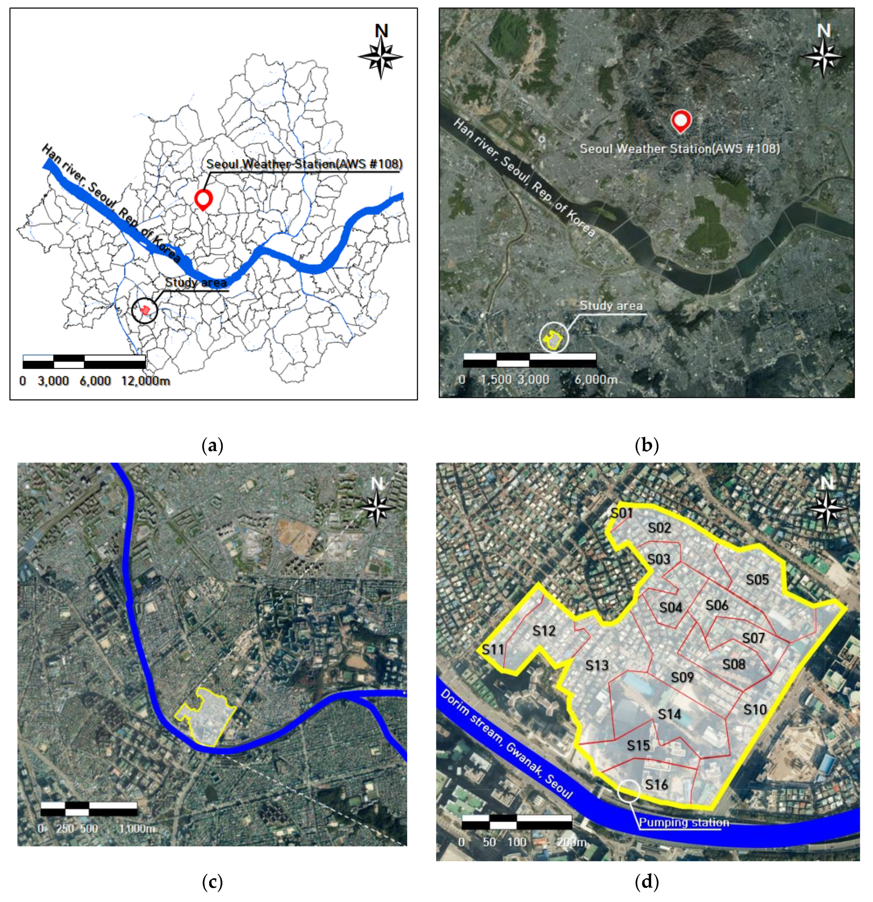
This study compared scenarios before and after installing LID facilities using synthetic rainfall at varying frequencies for an existing urban catchment sewer network system. The Daerim 2 rainwater pumping station catchment located near the Dorim Stream in Gwanak-gu, Seoul, was the target catchment in this study. Most of the catchment comprises densely populated urban residential areas. More detailed information on this catchment is listed in Figure 5 and

Table 4. Subcatchment Properties of the study area including the pumping station [58].

Category	Specification
Address	Dorimcheon-ro 21, Gwanak-gu, Seoul, Republic of Korea
Area (ha)	20.6
Number of nodes/links (EA)	34/34
Number of outlets (EA)	1
Watershed direction	The Dorim Stream of Korea
Pumping facilities	250 HP × 3 Pump (112 m3/min)
Pumping draining capacity(m3/min)	336

.

The runoff process of the urban catchment area varies depending on the land-use and several hydrological factors. Moreover, the runoff has a nonlinear rainfall–runoff relationship. An analysis model that accurately reflects the hydrologic parameters and the catchment situation is necessary to accurately simulate the change in the runoff quantity in urban catchments. This study applied the SWMM model commonly used worldwide for a detailed urban catchment analysis. The model parameters for the runoff quantity estimation of the catchment were selected based on the values presented in a 2010 report on the design and expansion of Daerim 3 pumping station [58]. Figure 6 shows the model construction.

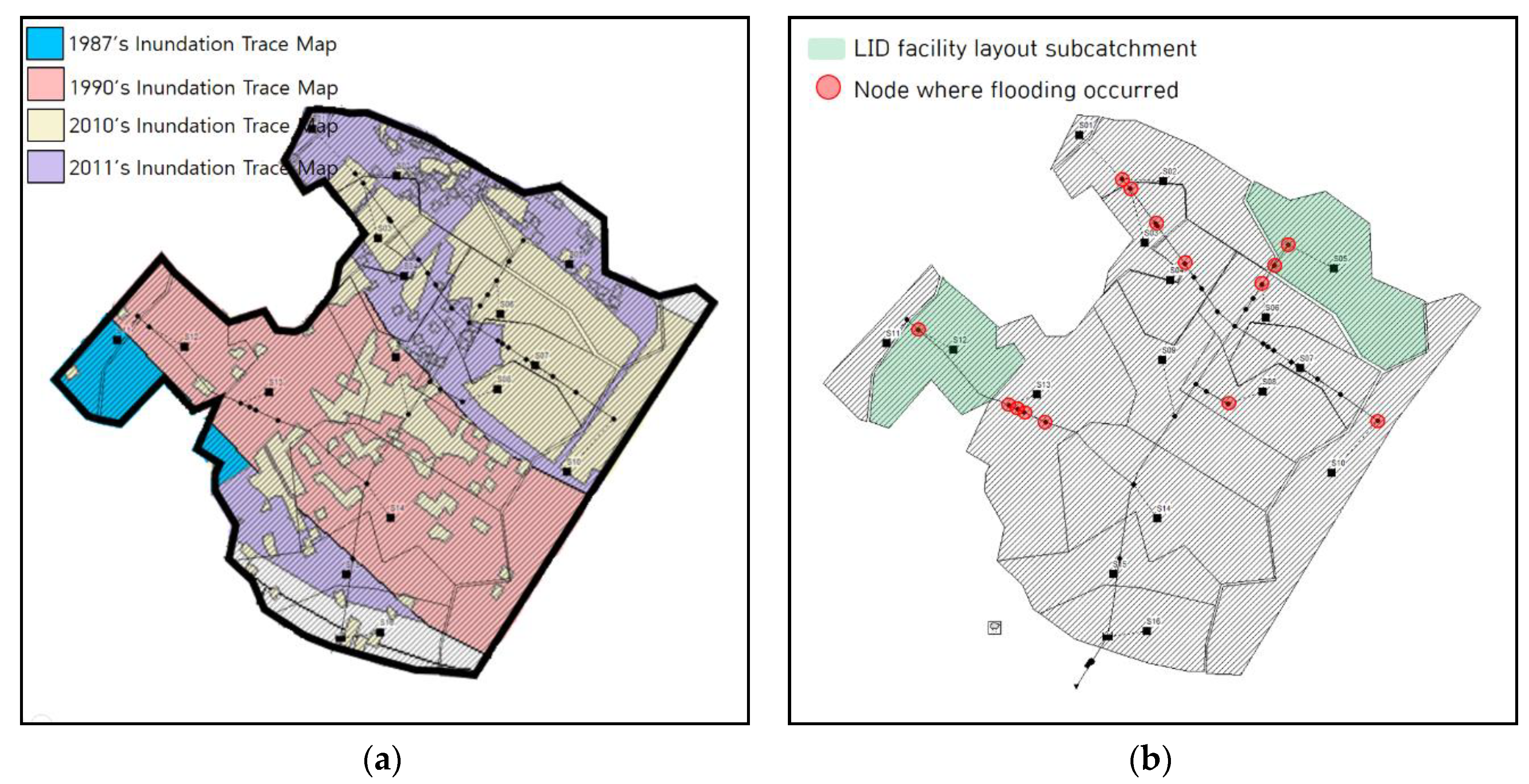
LID facilities were constructed for each catchment in the SWMM model. For the input, the number of applied LID facilities and the subcatchment area was divided and entered. Before classifying the number of applied LID facilities by subcatchment, subcatchments that required LID installation were examined. Initially, the inundation history in the catchment was reviewed using the Inundation Trace Map provided by the Seoul Information Communication Plaza (Figure 6a) [59]. Inundation Trace Map analysis confirmed inundation in subcatchment S05 in 2010 and 2011 and significant flood history. In the S12 subcatchment, overlaps occurred from the inundation trace maps in Seoul. The flood quantity simulation for each catchment was analyzed using the rainfall data in Table 1. This analysis revealed most of the flood quantity at the nodes near the S05 and S12 subcatchments. This result indicates the urgency of improving the subcatchment’s inundation and sewer networks. Figure 6b shows the results of flood occurrences considering rainfall events of 95.2 mm, with a design frequency of 70 years and a duration of 60 min. From this result, it is evident that most of the floods occur at the nodes near the S05 and S12 subcatchments. We also performed simulations for hypothetical scenarios assuming a single LID facility and 2–3 LID facilities.

2.8. Modeling Approach and Scenario

Seoul’s technical guidelines for the management of rainfall–runoff stipulate that districts with combined stormwater sewers must be treated using LID facilities by 2030 if one inch of the first flush occurs in approximately 10% of the impervious surface area [60]. The impervious areas for the 16 subcatchments considered in this study ranged from 900 to 1500 m². The LID facility area for each subcatchment was set to 1200 m², and eight scenarios were defined considering the existing sewer network system and three types of LID facilities. The details of these scenarios are outlined in

Table 5. Modeling approach and scenario conditions.

Scenario No.		Description (Combination of Facility)	Analysis Type
1	OG	Original Subcatchment Conditions	No LID
2	PP	Permeable Pavements (A = 1200 m2)	After LID (Type A)
3	GR	Green Roof (A = 1200 m2)
4	IT	Infiltration Trench (A = 1200 m2)
5	PP + GR	Permeable Pavements (A = 600 m2), Green Roof (A = 600 m2)	After LIDs (Type B)
6	PP + IT	Permeable Pavements (A = 600 m2), Infiltration Trench (A = 600 m2)
7	GR + IT	Green Roof (A = 600 m2), Infiltration Trench (A = 600 m2)
8	PP + GR + IT	Permeable Pavements (A = 400 m2), Green Roof (A = 400 m2), Infiltration Trench (A = 400 m2)

. Scenario 1 (OG) was analyzed based on the existing sewer network system configured for rainfall–runoff modeling. Scenario 2 (PP) reflected permeable pavements within the subcatchment. In this scenario, a single LID facility was assumed, and a facility area of 1200 m² per subcatchment was considered. Scenario 2 (GR) and Scenario 3 (IT) have the same assumptions as Scenario 1 and reflect green roofs and infiltration trenches in the LID facility areas. Scenario 5 (PP + GR), Scenario 6 (PP + IT), and Scenario 7 (GR + IT) assume multiple LID facilities, each with an area of 600 m². Scenario 8 (PP + GR + IT) includes all LID facilities considered in this study, with areas of 400 m².

3. Estimation of Reliability Index Factors

In this section, we describe the reliability calculation results of the sewer network system using DMM. We estimated the reliability of changes in the flood volume and flood nodes, BOD, and TSS. First, the results of R_V and R_N are described in

Table 6. Flood volume reliability calculations.

Flood Volume (Vi) (m3)
	Duration	Scenario 1 (OG)		Scenario 2 (PP)		Scenario 3 (GR)		Scenario 4 (IT)		Scenario 5 (PP + GR)		Scenario 6 (PP + IT)		Scenario 7 (GR + IT)		Scenario 8 (PP + GR + IT)
Frequency		30 min	60 min	30 min	60 min	30 min	60 min	30 min	60 min	30 min	60 min	30 min	60 min	30 min	60 min	30 min	60 min
30 years		4	0	4	0	4	0	4	0	4	0	4	0	4	0	4	0
50 years		22	0	18	0	18	0	18	0	18	0	18	0	18	0	18	0
70 years		98	271	49	39	49	42	56	102	49	39	54	82	54	84	53	61
80 years		136	468	87	277	87	280	97	318	87	280	95	311	95	312	96	301
100 years		230	734	181	578	179	582	188	623	180	578	185	602	185	604	183	600
Maximum Runoff Volume per minute (Ri × A) (m3)
	Duration	Scenario 1 (OG)		Scenario 2 (PP)		Scenario 3 (GR)		Scenario 4 (IT)		Scenario 5 (PP + GR)		Scenario 6 (PP + IT)		Scenario 7 (GR + IT)		Scenario 8 (PP + GR + IT)
Frequency		30 min	60 min	30 min	60 min	30 min	60 min	30 min	60 min	30 min	60 min	30 min	60 min	30 min	60 min	30 min	60 min
30 years		934.8	728.9	934.8	728.9	934.8	728.9	934.8	728.9	934.8	728.9	934.8	728.9	934.8	728.9	934.8	728.9
50 years		994.5	778.3	994.5	778.3	994.5	778.3	994.5	778.3	994.5	778.3	994.5	778.3	994.5	778.3	994.5	778.3
70 years		1034	809.2	1034	809.2	1034	809.2	1034	809.2	1034	809.2	1034	809.2	1034	809.2	1034	809.2
80 years		1046	821.5	1046	821.5	1046	821.5	1046	821.5	1046	821.5	1046	821.5	1046	821.5	1046	821.5
100 years		1073	842.1	1073	842.1	1073	842.1	1073	842.1	1073	842.1	1073	842.1	1073	842.1	1073	842.1
Vi/(Ri × A)
	Duration	Scenario 1 (OG)		Scenario 2 (PP)		Scenario 3 (GR)		Scenario 4 (IT)		Scenario 5 (PP + GR)		Scenario 6 (PP + IT)		Scenario 7 (GR + IT)		Scenario 8 (PP + GR + IT)
Frequency		30 min	60 min	30 min	60 min	30 min	60 min	30 min	60 min	30 min	60 min	30 min	60 min	30 min	60 min	30 min	60 min
30 years		0.004	0.000	0.004	0.000	0.004	0.000	0.004	0.000	0.004	0.000	0.004	0.000	0.004	0.000	0.004	0.000
50 years		0.022	0.000	0.018	0.000	0.018	0.000	0.018	0.000	0.018	0.000	0.018	0.000	0.018	0.000	0.018	0.000
70 years		0.095	0.335	0.047	0.048	0.047	0.052	0.054	0.126	0.047	0.048	0.052	0.101	0.052	0.104	0.051	0.075
80 years		0.130	0.570	0.083	0.337	0.083	0.341	0.093	0.387	0.083	0.341	0.091	0.379	0.091	0.380	0.092	0.366
100 years		0.214	0.872	0.169	0.686	0.167	0.691	0.175	0.740	0.168	0.686	0.172	0.715	0.172	0.717	0.171	0.712
{Vi/(Ri × A)}2
	Duration	Scenario 1 (OG)		Scenario 2 (PP)		Scenario 3 (GR)		Scenario 4 (IT)		Scenario 5 (PP + GR)		Scenario 6 (PP + IT)		Scenario 7 (GR + IT)		Scenario 8 (PP + GR + IT)
Frequency		30 min	60 min	30 min	60 min	30 min	60 min	30 min	60 min	30 min	60 min	30 min	60 min	30 min	60 min	30 min	60 min
30 years		0.000	0.000	0.000	0.000	0.000	0.000	0.000	0.000	0.000	0.000	0.000	0.000	0.000	0.000	0.000	0.000
50 years		0.000	0.000	0.000	0.000	0.000	0.000	0.000	0.000	0.000	0.000	0.000	0.000	0.000	0.000	0.000	0.000
70 years		0.009	0.112	0.002	0.002	0.002	0.003	0.003	0.016	0.002	0.002	0.003	0.010	0.003	0.011	0.003	0.006
80 years		0.017	0.325	0.007	0.114	0.007	0.116	0.009	0.150	0.007	0.116	0.008	0.143	0.008	0.144	0.008	0.134
100 years		0.046	0.760	0.028	0.471	0.028	0.478	0.031	0.547	0.028	0.471	0.030	0.511	0.030	0.514	0.029	0.508
Mean		0.127		0.062		0.063		0.076		0.063		0.071		0.071		0.069
SD		0.232		0.140		0.142		0.163		0.140		0.153		0.153		0.152
RV		0.873		0.937		0.937		0.924		0.937		0.929		0.929		0.931

and

Table 7. Flood node reliability calculations.

Flood Nodes (Ni)
	Duration	Scenario 1 (OG)		Scenario 2 (PP)		Scenario 3 (GR)		Scenario 4 (IT)		Scenario 5 (PP + GR)		Scenario 6 (PP + IT)		Scenario 7 (GR + IT)		Scenario 8 (PP + GR + IT)
Frequency		30 min	60 min	30 min	60 min	30 min	60 min	30 min	60 min	30 min	60 min	30 min	60 min	30 min	60 min	30 min	60 min
30 years		1	0	1	0	1	0	1	0	1	0	1	0	1	0	1	0
50 years		3	0	2	0	2	0	2	0	2	0	2	0	2	0	2	0
70 years		8	10	7	2	7	2	7	6	7	2	7	5	7	6	7	4
80 years		10	14	8	11	8	10	9	11	8	10	8	9	8	10	9	10
100 years		9	14	10	16	10	15	11	10	10	15	10	13	10	14	10	16
Total amount of rainfall (NT)
34 at all durations and frequencies
Ni/NT
	Duration	Scenario 1 (OG)		Scenario 2 (PP)		Scenario 3 (GR)		Scenario 4 (IT)		Scenario 5 (PP + GR)		Scenario 6 (PP + IT)		Scenario 7 (GR + IT)		Scenario 8 (PP + GR + IT)
Frequency		30 min	60 min	30 min	60 min	30 min	60 min	30 min	60 min	30 min	60 min	30 min	60 min	30 min	60 min	30 min	60 min
30 years		0.029	0.000	0.029	0.000	0.029	0.000	0.029	0.000	0.029	0.000	0.029	0.000	0.029	0.000	0.029	0.000
50 years		0.088	0.000	0.059	0.000	0.059	0.000	0.059	0.000	0.059	0.000	0.059	0.000	0.059	0.000	0.059	0.000
70 years		0.235	0.294	0.206	0.059	0.206	0.059	0.206	0.176	0.206	0.059	0.206	0.147	0.206	0.176	0.206	0.118
80 years		0.294	0.412	0.235	0.324	0.235	0.294	0.265	0.324	0.235	0.294	0.235	0.265	0.235	0.294	0.265	0.294
100 years		0.265	0.412	0.294	0.471	0.294	0.441	0.324	0.294	0.294	0.441	0.294	0.382	0.294	0.412	0.294	0.471
(Ni/NT)2
	Duration	Scenario 1 (OG)		Scenario 2 (PP)		Scenario 3 (GR)		Scenario 4 (IT)		Scenario 5 (PP + GR)		Scenario 6 (PP + IT)		Scenario 7 (GR + IT)		Scenario 8 (PP + GR + IT)
Frequency		30 min	60 min	30 min	60 min	30 min	60 min	30 min	60 min	30 min	60 min	30 min	60 min	30 min	60 min	30 min	60 min
30 years		0.001	0.000	0.001	0.000	0.001	0.000	0.001	0.000	0.001	0.000	0.001	0.000	0.001	0.000	0.001	0.000
50 years		0.008	0.000	0.003	0.000	0.003	0.000	0.003	0.000	0.003	0.000	0.003	0.000	0.003	0.000	0.003	0.000
70 years		0.055	0.087	0.042	0.003	0.042	0.003	0.042	0.031	0.042	0.003	0.042	0.022	0.042	0.031	0.042	0.014
80 years		0.087	0.170	0.055	0.105	0.055	0.087	0.070	0.105	0.055	0.087	0.055	0.070	0.055	0.087	0.070	0.087
100 years		0.070	0.170	0.087	0.221	0.087	0.195	0.105	0.087	0.087	0.195	0.087	0.146	0.087	0.170	0.087	0.221
Mean		0.065		0.052		0.047		0.044		0.047		0.043		0.048		0.053
SD		0.062		0.067		0.060		0.042		0.060		0.046		0.052		0.066
RN		0.935		0.948		0.953		0.956		0.953		0.957		0.952		0.947

. These results were calculated using synthetic rainfall events with a duration of 30 min and 60 min and five frequency types (30, 50, 70, 80, and 100 years) in the Daerim 2 rainwater pumping station catchment. An increase in rainfall increased the total flood quantity and total inflow to the sewer pipe network. Although overflow increased with the rise in rainfall event frequency, in the scenario considering LID facilities, reduced overflow risk is confirmed in Table 6 and Table 7.

The analysis results of synthetic rainfall events at a frequency of 30 and 50 years and a 60-min duration showed no overflow in the current sewer network system. Therefore, disaster risk was not represented in numbers in the reliability calculation process. The same finding applies to the results of flood volume and the number of flood nodes. However, the number of flood nodes decreased in Scenario 1 at a 100-year frequency because the sewer pipes’ design flow rate was exceeded, leading to a reduced burden on several nodes due to multiple overflow occurrences at the upstream nodes. This also resulted in the reduction of the reliability calculation to some extent. In the case of the overflow result, on average, in the installed scenario compared to Scenario 1 where the LID facility was not considered, the reduction effect of about 30% in the case of flood volume and about 18% in the case of the flood nodes occurrence was confirmed. The R_V and R_N values improved by 7% and 5%, respectively, according to the installation of the LID facility.

The reliability of R_V and R_N in Scenario 1, which did not consider LID facilities, was estimated at 0.873 and 0.935. For scenarios 2–8, which considered LID facilities, the reliability of R_V and R_N improved to 0.937 and 0.957. These results confirm the effect of inundation reduction for rainfall events exceeding design frequency through the implementation of LID facilities. When the R_V and R_N results were considered in combination, Scenario 4 was the most effective installation plan for flood disaster reduction. “Mean” and “SD” in Table 6, Table 7,

Table 8. BOD pollutant load reliability calculations.

BOD Pollutant Loads in Outfall (OB) (kg)
	Duration	Scenario 1 (OG)		Scenario 2 (PP)		Scenario 3 (GR)		Scenario 4 (IT)		Scenario 5 (PP + GR)		Scenario 6 (PP + IT)		Scenario 7 (GR + IT)		Scenario 8 (PP + GR + IT)
Frequency		30 min	60 min	30 min	60 min	30 min	60 min	30 min	60 min	30 min	60 min	30 min	60 min	30 min	60 min	30 min	60 min
30 years		0.020	0.017	0.016	0.014	0.016	0.014	0.015	0.014	0.016	0.014	0.015	0.014	0.015	0.014	0.015	0.014
50 years		0.020	0.017	0.016	0.014	0.016	0.014	0.016	0.014	0.016	0.014	0.016	0.014	0.016	0.014	0.016	0.014
70 years		0.021	0.017	0.016	0.014	0.016	0.014	0.016	0.014	0.016	0.014	0.016	0.014	0.016	0.014	0.016	0.014
80 years		0.021	0.017	0.016	0.014	0.016	0.014	0.016	0.014	0.016	0.014	0.016	0.014	0.016	0.014	0.016	0.014
100 years		0.021	0.017	0.016	0.014	0.016	0.014	0.016	0.014	0.016	0.014	0.016	0.014	0.016	0.014	0.016	0.014
BOD Pollutant Loads in the Total Subcatchment (LB) (kg)
	Duration	Scenario 1 (OG)		Scenario 2 (PP)		Scenario 3 (GR)		Scenario 4 (IT)		Scenario 5 (PP + GR)		Scenario 6 (PP + IT)		Scenario 7 (GR + IT)		Scenario 8 (PP + GR + IT)
Frequency		30 min	60 min	30 min	60 min	30 min	60 min	30 min	60 min	30 min	60 min	30 min	60 min	30 min	60 min	30 min	60 min
30 years		0.026	0.029	0.026	0.029	0.026	0.029	0.026	0.029	0.026	0.029	0.026	0.029	0.026	0.029	0.026	0.029
50 years		0.033	0.030	0.033	0.030	0.033	0.030	0.033	0.030	0.033	0.030	0.033	0.030	0.033	0.030	0.033	0.030
70 years		0.033	0.028	0.033	0.028	0.033	0.028	0.033	0.028	0.033	0.028	0.033	0.028	0.033	0.028	0.033	0.028
80 years		0.032	0.028	0.032	0.028	0.032	0.028	0.032	0.028	0.032	0.028	0.032	0.028	0.032	0.028	0.032	0.028
100 years		0.031	0.026	0.031	0.026	0.031	0.026	0.031	0.026	0.031	0.026	0.031	0.026	0.031	0.026	0.031	0.026
OB/LB
	Duration	Scenario 1 (OG)		Scenario 2 (PP)		Scenario 3 (GR)		Scenario 4 (IT)		Scenario 5 (PP + GR)		Scenario 6 (PP + IT)		Scenario 7 (GR + IT)		Scenario 8 (PP + GR + IT)
Frequency		30 min	60 min	30 min	60 min	30 min	60 min	30 min	60 min	30 min	60 min	30 min	60 min	30 min	60 min	30 min	60 min
30 years		0.770	0.583	0.616	0.480	0.616	0.480	0.577	0.480	0.616	0.480	0.577	0.480	0.577	0.480	0.577	0.480
50 years		0.604	0.569	0.483	0.469	0.483	0.469	0.483	0.469	0.483	0.469	0.483	0.469	0.483	0.469	0.483	0.469
70 years		0.644	0.606	0.490	0.499	0.490	0.499	0.490	0.499	0.490	0.499	0.490	0.499	0.490	0.499	0.490	0.499
80 years		0.660	0.617	0.503	0.508	0.503	0.508	0.503	0.508	0.503	0.508	0.503	0.508	0.503	0.508	0.503	0.508
100 years		0.676	0.645	0.515	0.531	0.515	0.531	0.515	0.531	0.515	0.531	0.515	0.531	0.515	0.531	0.515	0.531
(OB/LB)2
	Duration	Scenario 1 (OG)		Scenario 2 (PP)		Scenario 3 (GR)		Scenario 4 (IT)		Scenario 5 (PP + GR)		Scenario 6 (PP + IT)		Scenario 7 (GR + IT)		Scenario 8 (PP + GR + IT)
Frequency		30 min	60 min	30 min	60 min	30 min	60 min	30 min	60 min	30 min	60 min	30 min	60 min	30 min	60 min	30 min	60 min
30 years		0.000	0.000	0.000	0.000	0.000	0.000	0.000	0.000	0.000	0.000	0.000	0.000	0.000	0.000	0.000	0.000
50 years		0.000	0.000	0.000	0.000	0.000	0.000	0.000	0.000	0.000	0.000	0.000	0.000	0.000	0.000	0.000	0.000
70 years		0.009	0.112	0.002	0.002	0.002	0.003	0.003	0.016	0.002	0.002	0.003	0.010	0.003	0.011	0.003	0.006
80 years		0.017	0.325	0.007	0.114	0.007	0.116	0.009	0.150	0.007	0.116	0.008	0.143	0.008	0.144	0.008	0.134
100 years		0.046	0.760	0.028	0.471	0.028	0.478	0.031	0.547	0.028	0.471	0.030	0.511	0.030	0.514	0.029	0.508
Mean		0.127		0.062		0.063		0.076		0.063		0.071		0.071		0.069
SD		0.232		0.140		0.142		0.163		0.140		0.153		0.153		0.152
RB		0.798		0.838		0.838		0.840		0.838		0.840		0.840		0.840

and

Table 9. TSS pollutant load reliability calculations.

TSS Pollutant Loads in Outfall (OT) (kg)
	Duration	Scenario 1 (OG)		Scenario 2 (PP)		Scenario 3 (GR)		Scenario 4 (IT)		Scenario 5 (PP + GR)		Scenario 6 (PP + IT)		Scenario 7 (GR + IT)		Scenario 8 (PP + GR + IT)
Frequency		30 min	60 min	30 min	60 min	30 min	60 min	30 min	60 min	30 min	60 min	30 min	60 min	30 min	60 min	30 min	60 min
30 years		0.160	0.151	0.128	0.135	0.128	0.135	0.127	0.135	0.128	0.135	0.127	0.135	0.127	0.135	0.128	0.136
50 years		0.158	0.149	0.127	0.132	0.127	0.132	0.127	0.132	0.127	0.132	0.127	0.132	0.128	0.132	0.127	0.133
70 years		0.160	0.148	0.127	0.130	0.127	0.130	0.126	0.131	0.127	0.130	0.127	0.131	0.127	0.131	0.126	0.130
80 years		0.160	0.148	0.125	0.130	0.126	0.130	0.126	0.130	0.126	0.130	0.126	0.131	0.126	0.131	0.126	0.131
100 years		0.159	0.146	0.126	0.129	0.126	0.129	0.126	0.129	0.126	0.129	0.126	0.129	0.126	0.129	0.126	0.129
TSS Pollutant Loads in the Total Subcatchment (LT) (kg)
	Duration	Scenario 1 (OG)		Scenario 2 (PP)		Scenario 3 (GR)		Scenario 4 (IT)		Scenario 5 (PP + GR)		Scenario 6 (PP + IT)		Scenario 7 (GR + IT)		Scenario 8 (PP + GR + IT)
Frequency		30 min	60 min	30 min	60 min	30 min	60 min	30 min	60 min	30 min	60 min	30 min	60 min	30 min	60 min	30 min	60 min
30 years		0.215	0.224	0.215	0.224	0.215	0.224	0.215	0.224	0.215	0.224	0.215	0.224	0.215	0.224	0.215	0.224
50 years		0.243	0.231	0.243	0.231	0.243	0.231	0.243	0.231	0.243	0.231	0.243	0.231	0.243	0.231	0.243	0.231
70 years		0.244	0.223	0.244	0.223	0.244	0.223	0.244	0.223	0.244	0.223	0.244	0.223	0.244	0.223	0.244	0.223
80 years		0.240	0.220	0.240	0.220	0.240	0.220	0.240	0.220	0.240	0.220	0.240	0.220	0.240	0.220	0.240	0.220
100 years		0.232	0.210	0.232	0.210	0.232	0.210	0.232	0.210	0.232	0.210	0.232	0.210	0.232	0.210	0.232	0.210
OT/LT
	Duration	Scenario 1 (OG)		Scenario 2 (PP)		Scenario 3 (GR)		Scenario 4 (IT)		Scenario 5 (PP + GR)		Scenario 6 (PP + IT)		Scenario 7 (GR + IT)		Scenario 8 (PP + GR + IT)
Frequency		30 min	60 min	30 min	60 min	30 min	60 min	30 min	60 min	30 min	60 min	30 min	60 min	30 min	60 min	30 min	60 min
30 years		0.745	0.673	0.596	0.601	0.596	0.601	0.591	0.601	0.596	0.601	0.591	0.601	0.591	0.601	0.596	0.606
50 years		0.651	0.646	0.523	0.572	0.523	0.572	0.523	0.572	0.523	0.572	0.523	0.572	0.527	0.572	0.523	0.576
70 years		0.655	0.663	0.520	0.583	0.520	0.583	0.516	0.587	0.520	0.583	0.520	0.587	0.520	0.587	0.516	0.583
80 years		0.668	0.674	0.522	0.592	0.526	0.592	0.526	0.592	0.526	0.592	0.526	0.597	0.526	0.597	0.526	0.597
100 years		0.685	0.695	0.542	0.615	0.542	0.615	0.542	0.615	0.542	0.615	0.542	0.615	0.542	0.615	0.542	0.615
(OT/LT)2
	Duration	Scenario 1 (OG)		Scenario 2 (PP)		Scenario 3 (GR)		Scenario 4 (IT)		Scenario 5 (PP + GR)		Scenario 6 (PP + IT)		Scenario 7 (GR + IT)		Scenario 8 (PP + GR + IT)
Frequency		30 min	60 min	30 min	60 min	30 min	60 min	30 min	60 min	30 min	60 min	30 min	60 min	30 min	60 min	30 min	60 min
30 years		0.555	0.453	0.355	0.362	0.355	0.362	0.349	0.362	0.355	0.362	0.349	0.362	0.349	0.362	0.355	0.367
50 years		0.423	0.417	0.274	0.327	0.274	0.327	0.274	0.327	0.274	0.327	0.274	0.327	0.278	0.327	0.274	0.332
70 years		0.429	0.440	0.270	0.339	0.270	0.339	0.266	0.345	0.270	0.339	0.270	0.345	0.270	0.345	0.266	0.339
80 years		0.446	0.455	0.272	0.351	0.277	0.351	0.277	0.351	0.277	0.351	0.277	0.356	0.277	0.356	0.277	0.356
100 years		0.469	0.484	0.294	0.378	0.294	0.378	0.294	0.378	0.294	0.378	0.294	0.378	0.294	0.378	0.294	0.378
Mean		0.457		0.322		0.323		0.322		0.323		0.323		0.324		0.324
SD		0.038		0.039		0.038		0.039		0.038		0.039		0.038		0.040
RT		0.786		0.821		0.820		0.821		0.820		0.820		0.820		0.820

represents the average of reliability and standard deviation in 30 and 60 min, respectively.

Table 8 and Table 9 outlines the calculation results of R_B and R_T by analyzing the loads on water pollution. These results were calculated using synthetic rainfall events at 30 and 60 min and five frequency types (30, 50, 70, 80, and 100 years) in the Daerim 2 rainwater pumping station catchment. Evidently, the pollutant loads of BOD and TSS that occur in the catchment increase as the rainfall amount increases. Although the occurrence of pollutants increased with an increasing frequency of rainfall, the results of reducing the risk of water pollution in the scenario considering LID facilities are confirmed in Table 8 and Table 9.

The reason for the smaller result values of the BOD pollutant load in Table 8 compared to the TSS pollutant load values in Table 9 is possibly due to the dilution effect from the flow rate increase during transfer to the sewer pipes facility. For TSS, due to the characteristics of nonpoint source pollution in impervious areas during rainfall, pollutants scattered on the impervious surface during the non-rainfall period are introduced into sewer pipes at a high concentration by rainfall. The collected pollutants were discharged in proportion to the rainfall intensity, leading to a high cumulative pollutant load. This is possibly because the size of variation in the pollutant loads decreased with an increase in the rainfall amount. In the case of the water pollution result, on average, in the installed scenario compared to Scenario 1 where the LID facility was not considered, the reduction effect of about 20% in the case of BOD Pollutant Loads and about 16% in the case of the TSS Pollutant Loads occurrence was confirmed. The R_B and R_T values improved by 5% and 4%, respectively, according to the installation of the LID facility. The pollution load reduction pattern according to the change of the LID facility did not reach the flood reduction ratio. The sensitivity of the water pollution load according to the change of LID facilities did not change in proportion to the change of rainfall, and some facilities showed irregular patterns. In the case of LID facilities, the catchment area for each facility is the dominant function that determines the reduction rate of the pollution load rather than the difference in the diversity of facilities.

Pollutant loads were high before the overflow; however, the load values decreased following the typical pollutants’ concentration after the overflow. Therefore, the resultant values of the loads shown in this study do not vary significantly as the sewer flow rate increased rapidly following a sharp increase in surface water. Moreover, when analyzing the water pollution change using LID facilities, it is more typical to reflect long-term rainfall events based on time-series rainfall. However, in this study, the resultant values were small due to the consideration of short-duration rainfall with units in minutes. For identical values shown in Table 8 and Table 9, values may differ by decimal points. These differences can be observed in Table 9.

The reliability of R_B and R_T in Scenario 1, where LID facilities were not considered, was estimated at 0.798 and 0.786. In the results of scenarios 2–8, which consider LID facilities, the reliability of R_B and R_T improved to 0.840 and 0.821. These results confirm the effect of inundation reduction for rainfall events exceeding the design frequency through the implementation of LID facilities. When the results of R_B and R_T were considered in combination, Scenario 3 was the most effective installation plan for flood disaster reduction.

Table 10. Result of reliability index based on LID scenarios.

Result	Scenario 1 (OG)	Scenario 2 (PP)	Scenario 3 (GR)	Scenario 4 (IT)	Scenario 5 (PP + GR)	Scenario 6 (PP + IT)	Scenario 7 (GR + IT)	Scenario 8 (PP + GR + IT)
RV	0.8731	0.9375	0.9366	0.9244	0.9373	0.9294	0.9290	0.9312
RN	0.9354	0.9482	0.9527	0.9556	0.9527	0.9574	0.9524	0.9475
RB	0.7977	0.8384	0.8384	0.8399	0.8384	0.8399	0.8399	0.8399
RT	0.7862	0.8205	0.8204	0.8205	0.8204	0.8202	0.8201	0.8201
RFQD	0.8993	0.9426	0.9441	0.9380	0.9444	0.9417	0.9395	0.9388
RWQD	0.7919	0.8292	0.8292	0.8299	0.8292	0.8298	0.8297	0.8297
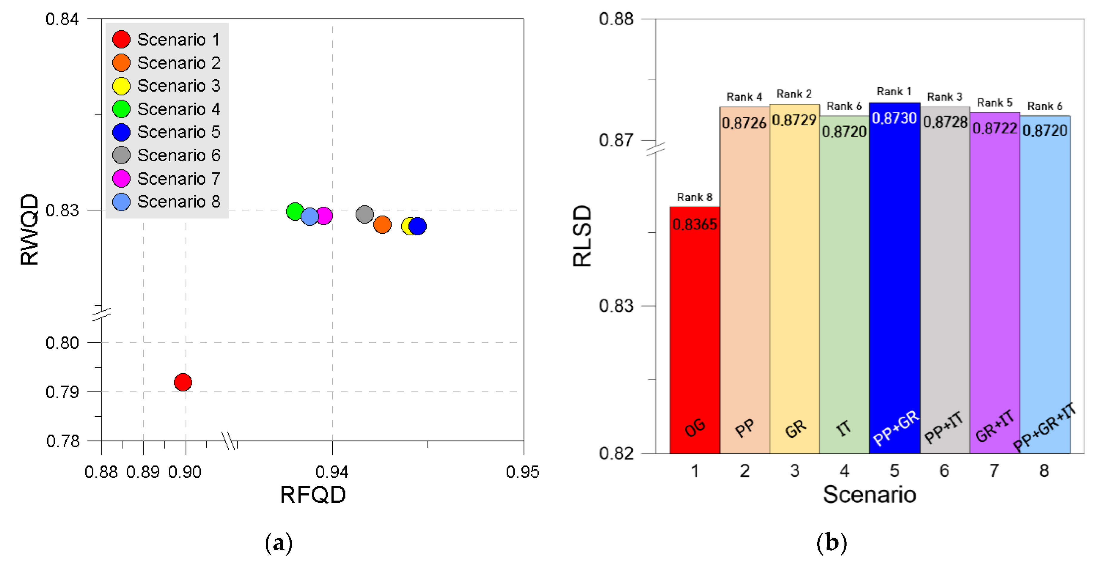
RLSD	0.8365	0.8726	0.8729	0.8720	0.8730	0.8728	0.8722	0.8720

is the calculation result of RLSD in combination with RFQS and RWQD. Figure 7 shows the results calculated per scenario. The RLSD value of the existing Daerim 2 rainwater pumping station catchment is 0.8365, and for scenario 5, in which LID facilities are reflected, we obtained an improved RLSD value of 0.8730 (+4.36%). This result indicates that applying a LID system reduced the existing flood quantity and the water pollution loads generated in the catchment.

Figure 7a demonstrates the reliability results of RFQD and RWQD. The graph indicates that the direct numbers could not have achieved the reliability improvement only because the variation in the improved reliability of the sewer network system in the various scenarios was small. However, evidently, as the risk of flood disaster and water pollution per scenario decreases, the reliability values gradually improve. For scenarios 4 and 8 in Table 10, although the evaluation index results for reliability evaluation items were the same, the different flood quantity and water pollution loads can be individually reflected, enabling a more quantitative reliability estimation of the sewer network system. Therefore, determining the reduction of overflow and pollutant loads confirmed the reduced values and established the actual phenomenon as a type of reliability through a quantitative number value of RLSD, as shown in Figure 7b.

In summary, the quantification of the reliability index in this study is theoretically significant and will help to minimize possible system function failures in the future. Moreover, the reliability indexing process plays an essential role in representing flood control performance and the current state of urban drainage systems The method proposed in this study can be used as a reference data and as a measurement tool for system quality in the risk assessment of urban inundation due to overflow occurrence and the quantification of the water pollution problem.

4. Conclusions

Frequent heavy rainfall events caused by climate change increase surface runoff quantity, leading to the degradation of the sewer network’s flood control function and efficiency. Furthermore, heavy rainfall exacerbates pollution problems from combined sewer overflows. Recently, the interest in managing nonpoint source pollution in urban catchments to improve the water quality of local rivers has increased. However, before this study, no research was conducted on a quantitative estimation method to facilitate flood disaster and nonpoint source pollution management. This study investigated the LID technique’s effectiveness in reducing inundation by improving the water cycle environment before urban development. Concerning the LID method, previous studies only considered the probability of system failure based on uncertainty analysis and did not examine system failure consequences.

In this study, the probability of failure for several scenarios was estimated using an evaluation method of the sewer network system and DMM as the reliability index. We defined the stormwater sewer system’s failure as the overflow and nonpoint source outflow due to synthetic rainfall. The flood volume and number of occurrence nodes for the sewer network system were used for overflow occurrence. For nonpoint source outflow, we used BOD and TSS pollutant loads to propose a reliability analysis method. We refer to this newly proposed index system as RLSD, and using DMM allows RLSD to comprehensively consider the reliability of flood disasters and water pollution, which have different dimensions.

However, depending on the difference in the return period of the applied rainfall events, rainfall duration, and rainfall distribution type, the pattern of overflow occurrence and the pollutant loads in the sewer network have different values. The different values cause a significant variation of the results. Therefore, assuming similar criteria, this study estimated the reliability by assigning the simulation results for each frequency and rainfall duration the same weight. However, the reliability result estimated by averaging may vary greatly depending on the criterion that reflects the amount of rainfall applied to the analysis. In this study, the degree of detail in the number and amount of rainfall to be considered was applied with limitations.

The RLSD proposed in this study can evaluate sewer pipe networks, but it is not sufficient for determining the absolute reliability of a single network. We recommend establishing a standard for a range of reliable values for a single pipe network, and further research on this topic is required. In addition, while RLSD can present the evaluation value for the entire system, it is impossible to evaluate maintenance holes and sewer pipes constituting the system, and further research in consideration of these elements is required. Besides, it is necessary to deal with a combination of system quantity and quality control performance measures. In this process, the model should be applied and verified using the actual official records as reference data. To increase the reliability of the study, we will consider a calculation-based approach to determine the cost of flood damage. To actively utilize this research method in the field, multi-purpose modeling considering various LID facilities and various results for it should be presented.

References

- IPCC. Synthesis Report. Contribution of Working Groups I, II and III to the Fifth Assessment Report of the Intergovernmental Panel on Climate Change; IPCC: Geneva, Switzerland, 2014; p. 151. [Google Scholar]
- Hirabayashi, Y.; Mahendran, R.; Koirala, S.; Konoshima, L.; Yamazaki, D.; Watanabe, S.; Kim, H.; Kanae, S. Global flood risk under climate change. Nat. Clim. Change 2013, 3, 816–821. [Google Scholar] [CrossRef]
- Rajapaksa, D.; Zhu, M.; Lee, B.; Hoang, V.N.; Wilson, C.; Managi, S. The impact of flood dynamics on property values. Land Use Policy 2017, 3, 317–325. [Google Scholar] [CrossRef]
- Alves, A.; Gersonius, B.; Kapelan, Z.; Vojinovic, Z.; Sanchez, A. Assessing the co-benefits of green-blue-grey infrastructure for sustainable urban flood risk management. J. Environ. Manag. 2019, 239, 244–254. [Google Scholar] [CrossRef] [PubMed]
- Ferguson, C.R.; Fenner, R.A. The potential for natural flood management to maintain free discharge at urban drainage outfalls. J. Flood Risk Manag. 2020, e2617. [Google Scholar] [CrossRef]
- Ebenstein, A. The consequences of industrialization: Evidence from water pollution and digestive cancers in China. Rev. Econ. Stat. 2012, 94, 186–201. [Google Scholar] [CrossRef] [Green Version]
- Elliott, A.H.; Trowsdale, S.A. A review of models for low impact urban stormwater drainage. Environ. Modell. Softw. 2007, 22, 394–405. [Google Scholar] [CrossRef]
- USEPA. Low Impact Development (LID), A Literature Review. USEPA Office of Water (4203), EPA-841-B-00-005, Washington, DC 20460. Available online: http://www.epa.gov/nps/lid/lidlit.html (accessed on 11 October 2019).
- Montalto, F.; Behr, C.; Alfredo, K.; Wolf, M.; Arye, M.; Walsh, M. Rapid Assessment of the Cost-Effectiveness of Low Impact Development for CSO Control. Landsc. Urban Plan. 2007, 82, 117–131. [Google Scholar] [CrossRef]
- National Stormwater Calculator User’s Guide; EPA/600/R-13/085; United States Environmental Protection Agency: Washington, DC, USA, 2013.
- Bouziotas, D.; van Duuren, D.; van Alphen, H.J.; Frijns, J.; Nikolopoulos, D.; Makropoulos, C. Towards circular water neighborhoods: Simulation-based decision support for integrated decentralized urban water systems. Water 2019, 11, 1227. [Google Scholar] [CrossRef] [Green Version]
- Madonsela, B.; Koop, S.; Van Leeuwen, K.; Carden, K. Evaluation of water governance processes required to transition towards water sensitive urban design—An indicator assessment approach for the City of Cape Town. Water 2019, 11, 292. [Google Scholar] [CrossRef] [Green Version]
- Fan, M.; Shibata, H.; Chen, L. Spatial priority conservation areas for water yield ecosystem service under climate changes in Teshio Watershed, Northernmost Japan. J. Water Clim. Chang. 2020, 11, 106–129. [Google Scholar] [CrossRef]
- Department of Environmental Resources. Programs, & Planning Division. In Low-Impact Development: An Integrated Design Approach; Department of Environmental Resource Programs and Planning Division: Prince George’s County, MD, USA, 1999. [Google Scholar]
- Wang, J.L.; Che, W.; Yi, H.X. Low impact development for urban stormwater and flood control and utilization. China Water Wastewater 2009, 16, 14. [Google Scholar]
- Zimmer, C.A.; Heathcote, I.W.; Whiteley, H.R.; Schroter, H. Low-Impact-Development Practices for Stormwater: Implications for Urban Hydrology. Can. Water Resour. J. 2007, 32, 193–212. [Google Scholar] [CrossRef]
- Hyland, S.E. Analysis of Sinkhole Susceptibility and Karst Distribution in the Northern Shenandoah Valley, Virginia: Implications for Low Impact Development (LID) Site Suitability Models. Ph.D. Thesis, Virginia Polytechnic Institute, Blacksburg, VA, USA, 2005. [Google Scholar]
- Dietz, M.E. Low impact development practices: A review of current research and recommendations for future directions. Water Air Soil Pollut. 2007, 186, 351–363. [Google Scholar] [CrossRef]
- Sadeghi, K.M.; Kharaghani, S.; Tam, W.; Gaerlan, N.; Loáiciga, H. Avalon green alley network: Low impact development (LID). In Proceedings of the World Environmental and Water Resources Congress, Los Angeles, CA, USA, 22–26 May 2016; pp. 205–214, Demonstration Project in Los Angeles. [Google Scholar]
- Ahiablame, L.M.; Engel, B.A.; Chaubey, I. Effectiveness of low impact development practices: Literature review and suggestions for future research. Water Air Soil Pollut. 2012, 223, 4253–4273. [Google Scholar] [CrossRef]
- Newman, G.; Sohn, W.M.; Li, M.H. Performance evaluation of low impact development: Groundwater infiltration in a drought prone landscape in Conroe, Texas. Landsc. Archit. Front. 2014, 2, 122–134. [Google Scholar]
- Guerra, H.B.; Kim, Y. Understanding the performance and applicability of low impact development structures under varying infiltration rates. KSCE J. Civ. Eng. 2020, 24, 1430–1438. [Google Scholar] [CrossRef]
- Ahiablame, L.M.; Engel, B.A.; Chaubey, I. Effectiveness of low impact development practices in two urbanized watersheds: Retrofitting with rain Barrel/Cistern and porous pavement. J. Environ. Manag. 2013, 119, 151–161. [Google Scholar] [CrossRef]
- Joksimovic, D.; Alam, Z. Cost efficiency of low impact development (LID) stormwater management practices. Procedia Eng. 2014, 89, 734–741. [Google Scholar] [CrossRef] [Green Version]
- Alfredo, K.; Montalto, F.; Goldstein, A. Observed and modeled performances of prototype green roof test plots subjected to simulated low- and high-intensity precipitations in a laboratory experiment. J. Hydrol. Eng. 2010, 15, 444–457. [Google Scholar] [CrossRef]
- Martin-Mikle, C.J.; de Beurs, K.M.; Julian, J.P.; Mayer, P.M. Identifying priority sites for low impact development (LID) in a mixed-use watershed. Landsc. Urban Plan. 2015, 140, 29–41. [Google Scholar] [CrossRef] [Green Version]
- Hatt, B.E.; Fletcher, T.D.; Deletic, A. Hydraulic and pollutant removal performance of fine media stormwater filtration systems. Environ. Sci. Technol. 2008, 42, 2535–2541. [Google Scholar] [CrossRef]
- Dietz, M.E.; Clausen, J.C. Stormwater runoff and export changes with development in a traditional and low impact subdivision. J. Environ. Manag. 2008, 87, 560–566. [Google Scholar] [CrossRef]
- Ahiablame, L.; Shakya, R. Modeling flood reduction effects of low impact development at a watershed scale. J. Environ. Manag. 2016, 171, 81–91. [Google Scholar] [CrossRef]
- Aerts, J.C.J.H.; Botzen, W.J.; Clarke, K.C.; Cutter, S.L.; Hall, J.W.; Merz, B.; Michel-Kerjan, E.; Mysiak, J.; Surminski, S.; Kunreuther, H. Integrating human behaviour dynamics into flood disaster risk assessment. Nat. Clim. Chang. 2018, 8, 193–199. [Google Scholar] [CrossRef] [Green Version]
- Schumann, G.J.; Brakenridge, G.R.; Kettner, A.J.; Kashif, R.; Niebuhr, E. Assisting flood disaster response with Earth observation data and products: A critical assessment. Remote Sens. 2018, 10, 1230. [Google Scholar] [CrossRef] [Green Version]
- Park, J.A. Risk Evaluation and Uncertainty Analysis in Urban Sewer System. Master’s Thesis, Daejin University, Pocheon, Korea, 2009. [Google Scholar]
- Campana, P.E.; Quan, S.J.; Robbio, F.I.; Lundblad, A.; Zhang, Y.; Ma, T.; Karlsson, B.; Yan, J. Optimization of a residential district with special consideration on energy and water reliability. Appl. Energy 2017, 194, 751–764. [Google Scholar] [CrossRef]
- Kowalski, D.; Kowalska, B.; Bławucki, T.; Suchorab, P.; Gaska, K. Impact assessment of distribution network layout on the reliability of water delivery. Water 2019, 11, 480. [Google Scholar] [CrossRef] [Green Version]
- Kumar, R.; Musuuza, J.L.; Van Loon, A.F.; Teuling, A.J.; Barthel, R.; Ten Broek, J.; Mai, J.; Samaniego, L.; Attinger, S. Multiscale Evaluation of the standardized precipitation index as a groundwater drought indicator. Hydrol. Earth Syst. Sci. 2016, 20, 1117–1131. [Google Scholar] [CrossRef] [Green Version]
- Sadeghfam, S.; Ehsanitabar, A.; Khatibi, R.; Daneshfaraz, R. Investigating ‘risk’ of groundwater drought occurrences by using reliability analysis. Ecol. Indic. 2018, 40, 170–184. [Google Scholar] [CrossRef]
- Lee, G.M. Water supply performance assessment of multipurpose dams using sustainability index. J. Korea Water Resour. Assoc. 2014, 47, 411–420. [Google Scholar] [CrossRef]
- Gouri, R.L.; Srinivas, V.V. A fuzzy approach to reliability based design of storm water drain network. Stoch. Environ. Res. Risk Assess. 2017, 31, 1091–1106. [Google Scholar] [CrossRef]
- Dauji, S. Reliability analysis for water supply distribution and storm water drainage systems: State of the art review. Clim. Chang. Environ. Sustain. 2019, 7, 3–13. [Google Scholar] [CrossRef]
- Lee, J.H. Development of a reliability estimation method for the storm sewer network. J. Korean Soc. Hazard Mitig. 2012, 12, 225–230. [Google Scholar] [CrossRef]
- Lee, J.H.; Park, M.J. A reliability evaluation method of storm sewer networks for excessive rainfall events. J. Korean Soc. Hazard Mitig. 2012, 12, 195–201. [Google Scholar]
- Lee, E.H.; Kim, J.H. Development of a reliability index considering flood damage for urban drainage systems. KSCE J. Civ. Eng. 2019, 23, 1872–1880. [Google Scholar] [CrossRef]
- Rossman, L.A.; Huber, W. Storm Water Management Model Reference Manual Volume I—Hydrology (Revised); United States Environmental Protection Agency: Cincinnati, OH, USA, 2016.
- Rossman, L.A.; Huber, W. Storm Water Management Model Reference Manual Volume II—Hydraulics; United States Environmental Protection Agency: Washington, DC, USA, 2017; 190p.
- USEPA. Storm Water Management Model User’s Manual Version 5.0; United States Environmental Protection Agency: Washington, DC, USA, 2010.
- Ministry of the Environment. Study on Appropriate Treatment & Management of the Public Sewage Treatment Works Entering the Industrial Wastewater; Ministry of the Environment: Sejong, Korea, 2011; Volume 50.
- Huff, F.A. Time distribution of rainfall in heavy storms. Water Resour. Res. 1967, 3, 1007–1019. [Google Scholar] [CrossRef]
- Korea Precipitation Frequency Data Server. Available online: www.k-idf.re.kr (accessed on 21 October 2020).
- Yoo, C.S.; and Na, W.Y. Analysis of a conventional Huff model at Seoul station and proposal of an improvisation method. J. Korean Soc. Hazard. Mitig 2019, 19, 43–55. [Google Scholar] [CrossRef]
- Rossman, L.A.; Huber, W.C. Storm Water Management Model Reference Manual Volume III—Water Quality; US Environmental Protection Agency: Wahshington, DC, USA; Office of Research and Development, National; Risk Book Company Management Laboratory: Cincinnati, OH, USA, 2016.
- Holzbauer-Schweitzer, B. Evaluating low impact development best management practices as an alternative to traditional urban stormwater management. Master’s Thesis, University of Oklahoma, Norman, OK, USA, 2016. [Google Scholar]
- Garsdal, H.; Mark, O.; Dørge, J.; Jepsen, S.E. Mousetrap: Modelling of water quality processes and the interaction of sediments and pollutants in sewers. Water Sci. Technol. 1995, 31, 33–41. [Google Scholar] [CrossRef]
- National Institute of Environment Research. Total Amount of Water Pollution Control Technology Guidelines; National Institute of Environment Research: Incheon, Korea, 2014.
- National Institute of Environment Research. Evaluation of Pollutants Reduction for Control of the Total Amount of Water Pollution; National Institute of Environment Research: Incheon, Korea, 2015.
- The Ministry of Environment of Korea. Sewage System Monitoring and Modeling Guidelines during Rainfall; Korea Environment Corporation: Incheon, Korea, 2018.
- Yeon, J.S.; Jang, Y.S.; Lee, J.H.; Shin, H.S.; Kim, E.S. Analysis of stormwater runoff characteristics for spatial distribution of LID element techniques Using SWMM. J. Korea Acad. Ind. Coop. Soc. 2014, 15, 3983–3989. [Google Scholar]
- Yeon, J.S. Estimation of Optimal Design Runoff Depth at Low Impact Development (LID) Facilities. Master’s Thesis, Department of Civil Engineering, Sun Moon University, Chungcheongnam-do, Korea, 2015. [Google Scholar]
- Seoul Metropolitan Government. Report on Design and Expansion of Daerim 3; Seoul Metropolitan Government: Seoul, Korea, 2010; pp. 54–58.
- Seoul Information Communication Plaza Data Server. Available online: http://opengov.seoul.go.kr (accessed on 24 August 2020).
- The Government of New York. Sustainable Stormwater Management Plan. Progress Report. Server. Available online: http://www.nyc.gov/html/planyc/downloads/pdf/publications/sustainable_stormwater_mgmt_plan_progress_report_october_2012.pdf (accessed on 24 August 2020).
Figure 1.
Research flowchart for runoff quantity and water quality reliability analysis of the low impact development (LID) system.
Figure 2.
Concept of LID construction based on catchment area.
Figure 3.
Concept of subcatchment classification according to LID facility application [45,46,47] (a) Before LID; (b) After LID (Type A); (c) After LIDs (Type B).
Figure 4.
Concept of utopian approach. (a) Utopian approach method using (b) the Euclidean distance of the two-vector concept [42].
Figure 5.
Basin and sewer network of Daerim2 pumping station. (a) GIS Map of the study area-Seoul, Rep. of Korea; (b) Map of the Seoul Weather Station (AWS #108); (c) Google Map Image of Daerim 2 Basin; (d) Its subcatchment Division (Map Data © 2020 Google, Imagery © 2020 CNES/Airbus, Maxar Technologies, NSPO 2020/Spot ImageMap Data © 2020 SK Telecom).
Figure 6.
Status of the two subcatchments reflecting LID facilities using the SWMM model: (a) Past flood plain maps of the study area; (b) Selection of subcatchments to install LID facilities.
Figure 7.
Result of reliability graph based on LID scenarios: (a) Reliability result points as a group of symbols scattered; (b) Reliability result points as a series of vertical bars.