Article

Real-Time Wave Excitation Forces Estimation: An Application on the ISWEC Device

1
Marine Offshore Renewable Energy Lab (MOREnergy Lab), DIMEAS, Politecnico di Torino, Corso Duca degli Abruzzi 24, 10129 Turin, Italy
2
Department of Mechanical Engineering, University of Bath, Bath 44210, UK
*
Author to whom correspondence should be addressed.
J. Mar. Sci. Eng. 2020, 8(10), 825; https://doi.org/10.3390/jmse8100825
Submission received: 3 October 2020 / Revised: 17 October 2020 / Accepted: 19 October 2020 / Published: 21 October 2020

Abstract

:
Optimal control strategies represent a widespread solution to increase the extracted energy of a Wave Energy Converter (WEC). The aim is to bring the WEC into resonance enhancing the produced power without compromising its reliability and durability. Most of the control algorithms proposed in literature require for the knowledge of the Wave Excitation Force (WEF) generated from the incoming wave field. In practice, WEFs are unknown, and an estimate must be used. This paper investigates the WEF estimation of a non-linear WEC. A model-based and a model-free approach are proposed. First, a Kalman Filter (KF) is implemented considering the WEC linear model and the WEF modelled as an unknown state to be estimated. Second, a feedforward Neural Network (NN) is applied to map the WEC dynamics to the WEF by training the network through a supervised learning algorithm. Both methods are tested for a wide range of irregular sea-states showing promising results in terms of estimation accuracy. Sensitivity and robustness analyses are performed to investigate the estimation error in presence of un-modelled phenomena, model errors and measurement noise.

1. Introduction

Among the different renewable sources, ocean waves represent one of the most powerful and in the last few decades have been widely investigated. Despite this, wave energy remains a relatively untapped resource. The application of Wave Energy Converter (WEC) systems to such irregular sources requires a robust control logic capable of maximizing the extracted energy with acceptable efficiencies. At present, the Optimal Control problem represents an active area of research. The work of [1] reports a comprehensive review of the advances in Optimal Control, Model Predictive Control (MPC) and MPC-like techniques applied to the wave energy field. Within the context of Optimal Control, accurate knowledge about the future Wave Excitation Force (WEF) is essential to compute the optimal control signal. In literature, several approaches have been proposed to address the problem of the WEF estimation with promising results. An exhaustive classification and comparison of several estimation techniques is presented in the work of [2]. Some examples are cited hereafter. In [3,4] a Kalman Filter (KF) observer is employed on a linear Point-Absorber (PA) WEC. It is assumed that the WEF can be modelled as a linear superposition of fixed and finite harmonic components. Similarly, In [5] the wave force estimation and prediction problem for arrays of WECs is approached, comparing both global and independent estimators and forecasters. In the work of [6] two approaches are presented: the first approach is based on a KF coupled with a random-walk model of the WEF; the second performs a receding horizon—unknown input estimation. In [7] a modified form of the well-known Fast Adaptive actuator Fault Estimation called Fast Adaptive Unknown Input Estimation (FAUIE) is applied to a non-linear PA. In [8] is studied a direct approach by measuring the pressures at discrete points on the buoy surface, in addition to the buoy heave position, to obtain the estimation of the WEF by an Extended Kalman Filter (EKF). Finally, In [9] studied the WEF estimation of WaveSub (by Marine Power Systems Ltd. (Swansea, England)), a multiple Degree of Freedom (DoF) non-linear WEC. The estimation problem is tackled with a stochastic and a periodic KF, using only quantities which are measurable in practice. A model-free approach is proposed by [10] emoploying a Neural Network (NN) framework to estimate the WEF on a PA. Similarly, In [11] is studied the estimation of the wave elevation using the measurements from a nearby buoy employing a Non-linear AutoRegressive with eXogenous input network (NARX). All the mentioned studies are promising in terms of estimation performances and robustness of the observer. However, most of the work cited refer to single Degree of Freedom (DoF) WECs and few studies on non-linear multiple DoF systems have been conduced so far.
The aim of this work is to estimate the WEFs on a non-linear three Degrees of Freedom (3-DoF) WEC using only readily measureable quantities to perform the estimation. The study is applied to the Inertial Sea Wave Energy Converter (ISWEC) device designed for the Mediterranean Sea. In this context, three different approaches have been applied to the ISWEC device in previous works. In [12] is built an unknown state observer with a second order augmented state space representation of the ISWEC for the estimation of the pitch excitation torque. The gain of the observer has been found with an LQR optimization. In [13] is presented a method to estimate the sea state Power Spectral Density (PSD) of the wave climate by using the device motion. The heave motion measurements are used to estimate the PSD of the incoming wave and the results compared with the wave PSD measured by a wave measurement system. Then, in [14] a feedforward NN is proposed to relate the ISWEC motion to the WEFs acting on surge, heave and pitch DoFs. In the current study two approaches are applied to the non-linear 3-DoF model of the ISWEC to estimate the WEFs acting on surge, heave and pitch DoFs:
  • Model-Based approach: a KF observer modelling the WEF as an unknown input with a harmonic nature. This estimation framework is studied in [3,4] and named Kalman Filter with Harmonic Oscillator (KFHO) in [2];
  • Model-Free approach: a feedforward NN to relate the ISWEC motion and gyroscopic reaction to the WEFs. The same approach reported in [14] is considered.
The main challenges lie in considering a non-linear 3-DoF model of the WEC and estimate the WEFs along three degrees of motion. In the KF context, tuning the system for the best performance in presence of measurement noise is crucial as well as identifying un-modelled phenomena and decoupling them from the signal to be estimated. Moreover, since the ISWEC device is slack-moored to the seabed, an accurate acquisition of the absolute displacements of the WEC is not trivial; in this context, measurement errors of the absolute diplacement could affect the estimation performances. For what concerns the NN, it is key to assess both the ability to estimate data that are not considered in the training process and the accuracy in presence of model uncertanities. The aim is to use the minimum amount of measurements to model the unknown exctitation forces in respect to the ISWEC kinematic. Outcomes of this investigation are the estimators performances in different irregular sea-states and different measurement frameworks in presence of sensors noises and plant uncertainties. The results of the 3-DoF KF estimator and the NN model are compared for different sensors framework in order to analyse the influence of the measurements available. Then, measurements noises and variations of the main plant parameters are introduced. Numerical simulations under different irregular sea conditions aim to compare the estimation results of the two approaches as well as the sensitivity to changes in the plant parameters relative to the case study presented. The novelty of this work is to perform an excitation force estimation for a 3-DoF non-linear WEC decoupling the mooring forces or, more in general, undesired phenomena that will appear in real operating condition. Moreover, the NN represents a novel framework to address the wave extitation force estimation problem, able to handle strong non-linearities. In the NN context, there are very few examples of application to a multi-DOF non-linear WEC system in literature. Finally, investigating the influence of available sensors constitutes a key aspect of this work, which aims to highlight the importance of having reliable measurements in the context of WEF estimation.
This paper is organized as follows. First, in 
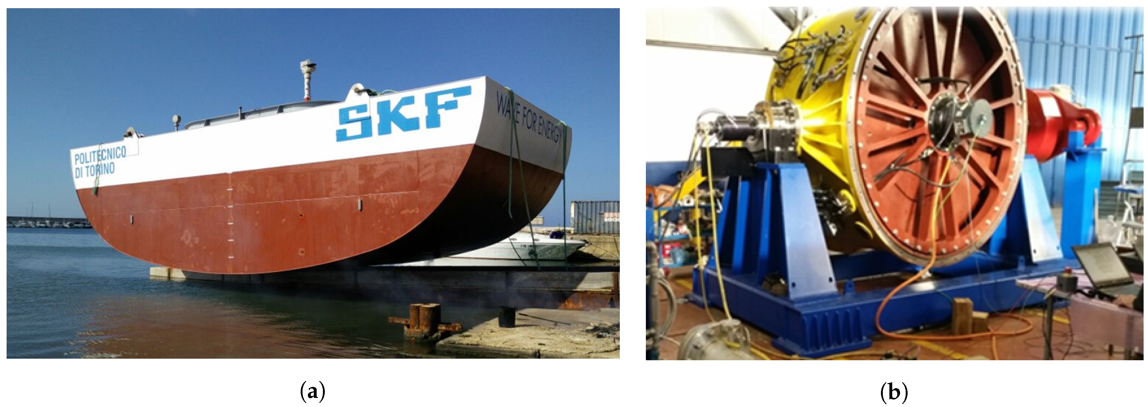
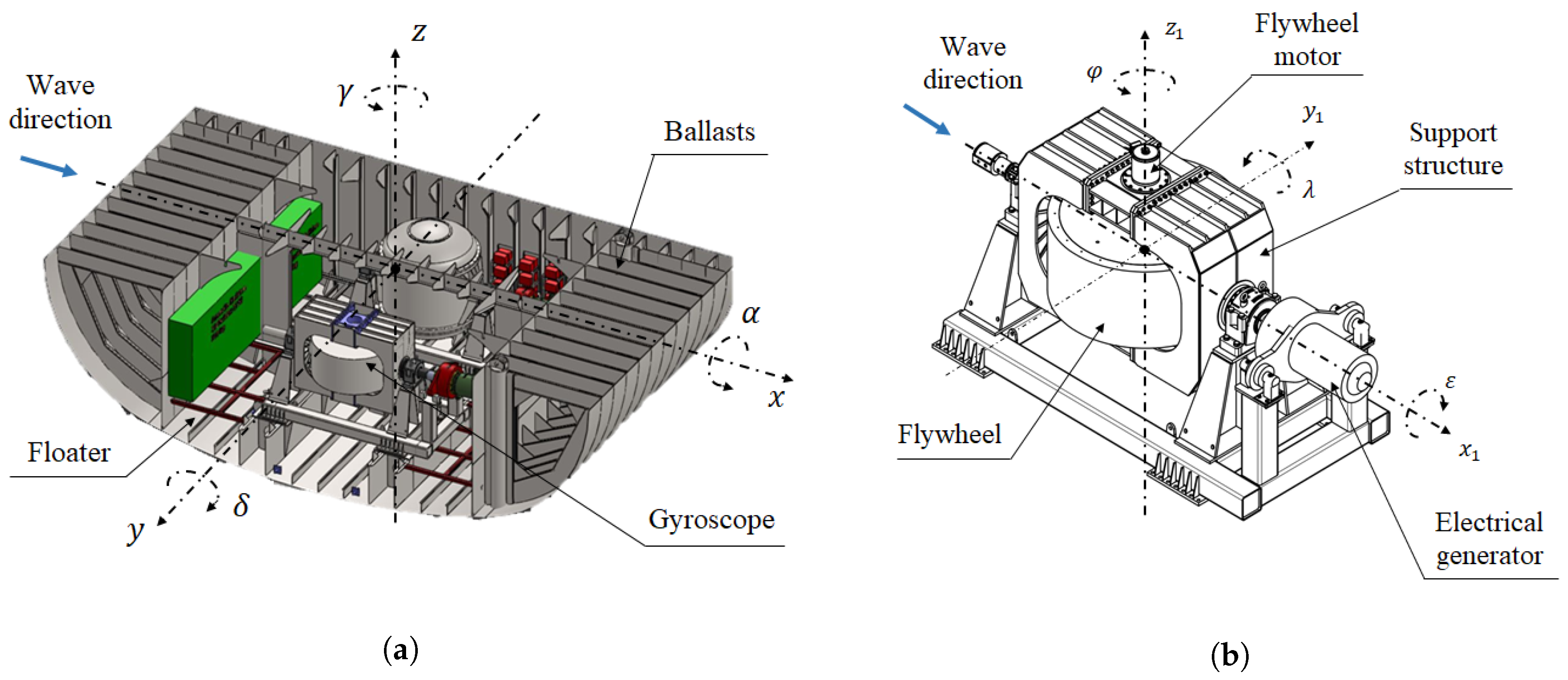
Section 2 the ISWEC architecture is described together with the non-linear 3-DoF time domain model. Second, Section 3 presents the linear 3-DoF ISWEC model in conjunction with the KF formulation used to estimate the WEFs. Section 4 describes the NN approach to estimate the WEFs as well as the network architecture. In Section 5 the parameters of both KF and NN are tuned considering the operating conditions of the ISWEC. Then, in Section 6, the numerical results are presented and discussed. Strengths and weaknesses of each method are compared and numerical experiments are used to assess estimation accuracy, robustness to different wave conditions, sensor noises and sensitivity to model errors. Finally, Section 7 presents conclusions and future works.

2. ISWEC Device

The ISWEC system has been considered as the case study in this paper. The first concept is dated 2005, conceived by the renewable group of the Department of Mechanical and Aerospace Engineering of the Politecnico di Torino (Italy). In 2012, a 1:8 prototype was realized and tested at INSEAN wave tank in Rome, crucial to draw the main guidelines for the ISWEC design. In 2012, the design of a 60 kW rated power ISWEC full-scale prototype (shown in Figure 1) started and the device has been installed in Pantelleria island (Sicily, Italy) in Summer 2015. The project aimed to evaluate the device energy production capabilities and efficiency. In 2018, a new collaboration with the Italian company Eni S.p.a. led to the construction of a second full-scale prototype in the early 2019, installed in the Adriatic Sea (Italy). This second full-scale prototype maintains the architecture and operating principle of the Pantelleria device. The development of more accurate numerical models together with ad hoc optimization algorithms validated and supported by the experimental data of the Pantelleria device enabled efficiency and reliability improvements to the overall device. In this section the device working principle and the non-linear 3-DoF numerical model refer to the prototype installed in Adriatic Sea.

2.1. ISWEC Working Principle

The major disadvantage of PA-like devices is that they harness wave energy damping directly from the motion of an oscillating buoy, exploiting the relative motion of mechanical parts in contact with the harsh marine environment. The idea of the ISWEC is to harvest wave energy damping from the floater motion through a gyroscope system which is protected within the hull, reducing the risk of corrosion and biofouling, with consequent increase of reliability. Morevoer, also the power conversion and conditioning systems are completely enclosed into the floater. The only part that have continuity from the inside out is the electric cable, following the idea of a “deploy and plug” device [15]. A schematic representation of the device concept is shown in Figure 2. It consists of a sealed hull carrying inside two gyroscopic units. The power conversion principle relies on the gyroscopic effect that converts the pitching angular motion of the hull into an inner precession oscillation of the gyroscopes. ISWEC is a directional WEC since, in normal working conditions, it is able to align itself with the wave direction. As shown in Figure 2b, the gyroscope is composed of a spinning flywheel that rotates around the z 1 axis with a speed φ ˙ . The flywheel is supported by a frame that allows the rotation of the gyroscope around its precession axis x 1 . The precession motion is excited through the dynamic coupling between the hull motion around the y 1 axis and the flywheel angular velocity around the z 1 axis. A mechanical gearbox and an electrical generator, connected to the gyroscopic frame, compose the electrical Power Take-Off (PTO). Two electrical generators extract electricity acting as a linear damper braking the precession motion of the gyroscope. Notwithstanding the energy required to keep the flywheel in rotation, the possibility to regulate its speed along with the tuning of the PTO torque allows the adaptation of the natural resonant frequency of the system to the incoming wave. An accurate description of the internal components and their working principle can be found in the works of [15,16,17].

2.2. ISWEC Non-Linear Time Domain Model

The ISWEC mathematical model is obtained by coupling the hull hydrodynamics and the gyroscope dynamics. The non-linear system equations have been implemented in the MATLAB®/Simulink® environment employing the Simscape™ Multibody™ toolbox, which is particularly suitable for multi-physics system modelling. The derivation and the experimental validation of the model equations of the complete system is not within the scope of this work and details can be found in the studies of [18,19,20,21].
WEC modelling is the major area of interest within the field of Wave Energy. Multitudes of WEC models are proposed in literature with different levels of confidence and uncertainties [22,23]. In this work, the fluid-structure interaction model is based on linear potential flow theory under the assumptions of irrotational flow, inviscid and incompressible fluid, harmonic oscillations of the hull for each DoF and zero-forward-speed conditions [24]. Then, according to the well-known Cummins’ equation [25], the dynamic behaviour of a floating body can be derived in the time domain. Some non-linear effects are considered: the non-linear viscous forces, the drift forces in the surge direction, the mooring action and the gyroscopic reaction on the hull. As stated in the previous paragraph, the ISWEC device extracts energy from the sea exploiting only the motion around the pitch axis. Moreover, the hull is symmetrical with respect to its longitudinal and transversal plane. Under these assumptions, a planar 3-DoF model of the hull has been considered in this work. The reference plane is identified by the vertical gravity axis z and the horizontal direction of the incoming wave x as shown in Figure 2a. Let X f ( t ) R n D be the vector containing the n D DoFs of the hull:
X f ( t ) = x ( t ) z ( t ) δ ( t ) T
Then, X ˙ f ( t ) R n D and X ¨ f ( t ) R n D are the first- and second-time derivative of X f respectively. In a planar reference frame, x ( t ) represents the surge motion, z ( t ) the heave motion and δ ( t ) the pitch motion. Following the notation of Equation (1), the time-domain equation of the hull dynamics can be written as follows:
M X ¨ f ( t ) + F r ( t ) + F β ( t ) + K X f ( t ) = F w ( t ) + F d ( t ) + F m ( t ) + F g ( t )
where M R n D × n D is the mass matrix including the added mass contribution evaluated for infinite oscillation frequency, F r ( t ) R n D are the radiation forces, F β ( t ) R n D the non-linear viscous forces, K R n D × n D the linear hydrostatic stiffness, F w ( t ) R n D the wave exctitation forces, F d ( t ) R n D the non-linear wave drift forces, F m ( t ) R n D the mooring line actions and F g ( t ) R n D the gyroscopic reactions on the hull. For the sake of clarity, the subscripts x, z and δ will be used in the next sections to specify the DoF to which the force or parameters refer and the subscript j to indicate the j-th DoF.

2.2.1. Radiation Convolution Term

The radiation forces arise from the motion of the hull through the water that results in inertia and friction components. These contributions can be obtained by solving the convolution integral of the impulse response function h r ( t ) [26]:
F r ( t ) = 0 t h r ( t τ ) X ˙ f ( τ ) d τ
As the computation of the convolution integral can be very time consuming, it is convenient to express this term with a state-space representation:
ζ ˙ ( t ) = A r ζ ( t ) + B r X ˙ f ( t ) F r ( t ) = C r ζ ( t ) + D r X ˙ f ( t )
The vector ζ ( t ) R n R represents the state vector that approximates the radiation force contributions and n R is the approximation order. The state space matrices A r R n R × n R , B r R n R × n D , C r R n D × n R and D r R n D × n D have been identified following the well-known Perez and Fossen and approach [26,27].

2.2.2. Non-Linear Viscous Forces

For evaluating the non-linear viscous forces F β , [28] proposed a method for the identification of the viscous force for the pitch DoF:
F β δ ( t ) = β δ ˙ ( t ) | δ ˙ ( t ) |
The method relies on a full CFD approach through which a pitch free decay test is simulated. Once the time series is obtained, it is possible to identify the viscous damping coefficient β with two different methodologies: computing the viscous damping coefficients through the logarithmic decrement method and/or integrating the Cummins’ equation of motion fitting the damping coefficients that minimize the difference with CFD results. In the surge direction, The work of [29] evaluated the viscous force according to the drag force contribution of the Morison equation, assuming the hypothesis of low forward speed:
F β x = 1 2 ρ C d A x ˙ ( t ) | x ˙ ( t ) |
In Equation (6), ρ represents the water density, C d the drag coefficient and A the wetted area of the hull. The drag coefficient formulation can be found in literature for simple geometries. The viscous damping in the heave direction is not considered since the hull motion along the vertical axis does not contribute to the power extraction in this WEC. Moreover, it is decoupled for the surge and pitch DoFs due to the symmetry of the hull on the transversal plane.

2.2.3. Drift Forces

The drift force is required in order to describe properly the hydrodynamic behaviour of the hull along the surge DoF. The derivation of this action for the ISWEC device can be found in the work of [29]. Here the time series of wave drift force for irregular sea state were derived through the Newman approximation [30]:
F d x ( t ) = 2 h = 1 W η h f d ( ω h ) c o s ( ω h t + θ h ) 2
where the subscript h indicates the h-th harmonic component of the wave spectrum, W is the number of frequencies of the spectrum discretization, η h the harmonic amplitude of the wave spectrum, f d ( ω h ) the drift force coefficient for each frequency component ω h of the wave spectrum and θ h the phase angle.

2.2.4. Mooring System

The mooring system is modelled through a quasi-static approach following the formulation proposed by [29]. The static equilibrium of the system is studied by varying the x coordinate and the z coordinate of the connection point of the mooring to the hull. Then, computing the equilibrium condition of the mooring line for all the different possible positions of the device, the mooring tensions are identified. In the numerical model, F m is obtained with MATLAB® look-up tables that map the mooring forces in respect to the hull planar motion. As shown in Figure 3, the ISWEC mooring system consists of a slack catenary type with multiple mooring lines, jumpers and clump-weights. Two bridles connect the hull to a central joint to prevent the roll motion of the device. To guarantee the weather-vaning of the device in respect to the wave direction, the mooring connection points are placed towards the bow, with respect to the centre of gravity of the device. On each catenary, a sub-surface buoy and clump-weight are installed to enhance the elastic recall of the system and avoid snatches [31].

2.2.5. Gyroscope Reactions

The gyroscope dynamics can be described through the Newton’s law and derived from the conservation of the flywheel angular momentum. The non-linear numerical model considers all the contributions of the gyroscope reaction along the x, z and δ DoFs. Through a linearization of the angular momentum of the gyroscope around the y 1 axis, the expression of the gyroscopic reaction discharged on the pitch DoF of the hull can be determined [32]:
F g δ ( t ) = J φ ˙ ε ˙ ( t ) c o s ( ε ( t ) )
where J is the flywheel moment of inertia, and ε ˙ ( t ) and ε ( t ) are the gyroscope speed and angular position around the precession axis y 1 , respectively. This torque acts on the pitch axis representing the third component of the F g term in Equation (2). In this work, the gyroscope reaction is considered as a known input of both KF and NN as it can be computed through the measurements of the gyroscope kinematics. The complete derivation of the gyroscope dynamic equation can be found in [32].

2.2.6. Wave Excitation Force Modelling

The linear wave theory describes the irregular water surface as superposition of harmonic waves with different frequencies, phases and directions [33,34]. In this work, only unidirectional waves are considered since the ISWEC device is described only in its longitudial plane. Then, the wave signal can be approximated through a Fourier series of any arbitrary number N of harmonic wave components [35]:
η ( t ) = n = 1 N A n c o s ( ω n t + α n )
where A n is the amplitude, ω n the angular frequency and α n the n-th phase associated with the n-th harmonic. Traditionally, Power Spectral Densities (PSD) of real waves are modelled analytically and parametrized according to their spectral properties. In literature, different analytical PSD functions are proposed. Given the wave spetrum, the amplitude of the sinusoidal n-th wave component of η ( t ) is obtained by the following relation [35]:
η n = 2 S η η ( ω n ) Δ ω
where Δ ω is the PSD frequency resolution and S η η is the value of spectral energy density. Therefore, the WEF associated to the j-th DoF can be calculated given the geometry of the floater and sea-state characteristics [36]:
F w j ( t ) = n = 1 N | f j ( ω n ) | η n c o s ( ω n t + θ n + f j ( ω n ) )
where f j ( ω n ) is the Froude-Krylov and diffraction coefficient associated to the j-th DoF and the n-th wave frequency. In this work, the Joint North Sea Wave Project (JONSWAP) spectrum [37] is considered to define 35 different irregular sea-states to evaluate the estimation performances. However, only four sea-states are employed to tune the KF and NN models according to the operating conditions of the ISWEC device. The JONSWAP spectrum can be identified using three parameters: Significant wave Height ( H s ), Energy Period ( T e ) and Peak Shape ( γ ). These spectral parameters are reported in Table 1 for each sea-states used for the tuning process, sorted in ascending order of wave Power density ( P d ).
Figure 4 gives a qualitative representation of annual wave energy of the sea-states considered. Data refer to a typical annual distribution of the wave energy in the Adriatic Sea (Italy) acquired during an experimental campaign started in 2018. The data are normalized on their maximum value. The squared blue marker represents the four waves used for the tuning process.

2.2.7. Sensor and Acquisition System Model

The ISWEC device installed in the Adriatic Sea is equipped with a Data AcQuisition (DAQ) system to record experimental signals of the physical quantities of interest. The motion of the three DoFs of interest of the hull has to be acquired. Moreover, to complete the estimation the precession motion of the gyroscope as well as the flywheel speed are required. The linear accelerations, angular orientations and rates of the hull are provided by an Inertial Unit of Measurement (IMU) Xsens MTi-30 AHRS [38] fixed inside the floater. The sensor is rigidly fixed inside the hull, appropriately oriented in respect to the hull reference system. An internal data processor uses the velocity and orientation increments and, through a strapdown integration algorithm, gives in output the orientations on the three rotational DoFs. The measurements considered from the IMU are: the linear acceleration along the surge and heave directions ( x ¨ ( t ) and z ¨ ( t ) ), the angular position and velocity of the hull ( δ ( t ) and δ ˙ ( t ) ). Two digital encoders Heidenhain Ecn 413 [39] are mounted on the gyroscope and flywheel shaft, respectively. The measurements available from the encoders used for computing the gyroscope reaction F g ( t ) are: the flywheel speed ( φ ˙ ( t ) ), the angular position and speed of the gyroscope ( ε ( t ) and ε ˙ ( t ) ). The data acquisition is managed by a National Instrument compactRIO NI cRIO-9030 [40] which is a dual core 1.33 GHz real time control unit. These sensors and hardware, together with temperature, umidity, voltage and current measurements compose the actual ISWEC DAQ.
Unlike the majority of PA type WECs, the ISWEC device is slack-moored to the seabed and a precise measure of its absolute position is not trivial. In this context, a Differencial GPS (DGPS) is considered to acquire the position and elevation of the WEC. The differential positioning technique enhance the GPS position accuracy of geo-location by comparing their data with those recorded in the same time interval by other multiple GPS receivers. The measurements given by the DGPS are: the position x ( t ) and the elevation z ( t ) . The measures of IMU and DGPS can be combined to perform the well-known sensor fusion technique [41,42]. Sensor fusion represents a foundamental part of localization and position tracking and can be applied to estimate the absolute positions and velocities with high accuracy. In this context, Motion Reference Units (MRU) are meant for measuring positions, velocities, accelerations, angular rates and orientations representing an all-in-one solution for acquiring the WEC motion. The MRU are more precise than IMU units and returns absolute positions and velocities relative to a specified equilibrium point. These sensors are employed in modern navigation systems and dynamic positioning applications. The measurements available from the MRU are: the positions ( x ( t ) and z ( t ) ), velocities ( x ˙ ( t ) and z ˙ ( t ) ) and acceleration ( x ¨ ( t ) and z ¨ ( t ) ) along the surge and heave directions, the angular position and velocity of the hull ( δ ( t ) and δ ˙ ( t ) ). Table 2 reasumes all the frameworks considered in this work and their noise standard deviations σ .
The Full Measurements (FM) configuration represent an ideal measurement framework in which all measures are available. Filled black dots in Table 2 indicates that the FM framework considers measurements without noise. This framework is the referance case where maximum estimation performances are expected. The angular acceleration along the pitch DoF δ ¨ ( t ) is not considered since none of the available sensors provide it. Encoders data are considered available for all the configurations. It is worth pointing out that missing measurements in IMU+DGPS and IMU frameworks can be obtained by numerical derivation/integration of position, velocity and acceleration signals. However, in this work, only raw measurements obtained directly from the sensors are considered.

2.3. ISWEC Model Block Diagram

The block diagram of the ISWEC plant is shown in Figure 5. The input of the system are the Wave Excitation Force F w ( t ) and the Wave Drift Fore F d ( t ) . First, the Equation (2) is integrated inside the block Hull. The output of this block are the hull positions X f ( t ) , velocities X ˙ f ( t ) and accelerations X ¨ f ( t ) that represent the input of the Gyroscope block. Here the dynamic equation of the gyroscope is solved computing the gyroscope motion ε ( t ) and ε ˙ ( t ) around the precession axis and the gyroscope reaction F g ( t ) that is feedback to the Hull. The Mooring block computes the recall F m ( t ) in respect to the hull position X f ( t ) . Then, the block Power Take-Off computes the generator torque T ε ( t ) and sends feedbacks back to the Gyroscope. The control algorithm implemented by the Power Take-Off is described in detail in [15]. The motion of the hull is acquired through the IMU [38] and the gyorscope and flywheel angular speeds with two Encoders [39]. The measurements are tainted with noise w I M U ( t ) and w E ( t ) and sampled at 10 Hz with the cRIO unit [40] to obtain the discrete data with pedix d.

3. Wave Excitation Force Estimation with Kalman Filter

One solution to estimate the WEF could be measuring directly the pressure acting on the wetted surface of the hull [8]. However, this method could be expensive as it requires a large number of sensors. Furthermore, since the pressure measured on the wetted surface is the combination of all the hydrodynamics forces it could be challenging to distinguish the contribution of the WEF. Another method relies on the measurement of the hull dynamics and an estimation is performed. The KF is ubiquitous in many applications to estimate the current state of a linear dynamic system from a set of measurements affected by uncorrelated Gaussian noise with known covariance. Under these assumptions, this estimator is defined as optimal because it estimates the system states minimizing the covariance of the estimation error. In this work, the estimation procedure is carried out by modelling the WEF as an unknown state to be estimated [4]. In order to obtain the KF formulation the Equation (2) is taken into account. First, the non-linear model is simplified considering the drift forces included into the F w x ( t ) contribution. The viscous damping along the pitch direction is linearized and the surge damping action is neglected in order to obtain a 3-DoF linear state space model. Then, the state space model of the ISWEC is discretized in the time domain to derive the KF formulation. The mooring forces are identified and the filter is designed to decouple them from the WEF. These steps are described in detail in the following sub-sections.

3.1. Linear 3-DoF ISWEC Model

The non-linear model described in the previous chapter is simplified to achieve a compromise between the computational effort required to solve the KF algorithm and the accuracy of the estimation. The non-linear viscous force along the pitch DoF defined by Equation (5) has to be linearized for inclusion in the estimation process. Four simulations are performed in four different sea-states using the non-linear 3-DoF numerical model and wave data of Table 1. The pitching rate amplitude time series is extracted and its mean is computed for each simulation. The mean is substituted into Equation (5) and β l i n is defined as the product between the viscous damping β and the mean pitching amplitude:
F β δ ( t ) β δ ¯ ˙ δ ˙ ( t ) = β l i n δ ˙ ( t )
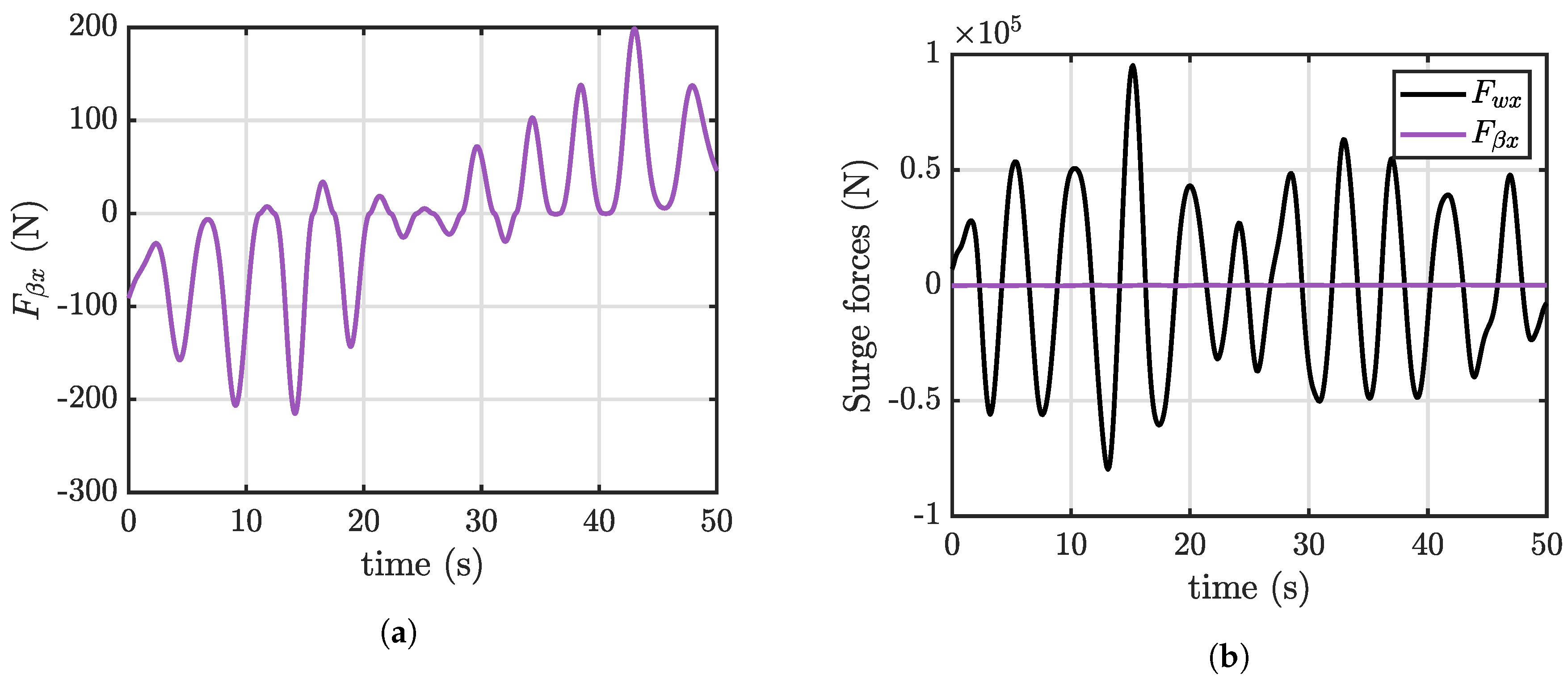
For the surge direction, Figure 6 demonstrates that the viscous force along the surge DoF can be neglected in respect to the WEF.
The term F β ( t ) can be rewritten as:
F β ( t ) 0 0 0 0 0 0 0 0 β l i n X ˙ f ( t ) = B v X ˙ f ( t )
Substituting the Equation (13) in (2), Equation (2) can be expressed by the following linear continuous-time state-space model:
X ˙ ( t ) = A X ( t ) + B F g ( t ) + B [ F w ( t ) + F m ( t ) ] Y ( t ) = C X ( t ) + D F g ( t ) + D [ F w ( t ) + F m ( t ) ]
where X ( t ) R n S and Y ( t ) R m S are the states and measurements vectors defined as:
X ( t ) = X f ( t ) X ˙ f ( t ) ζ T Y ( t ) = X f ( t ) X ˙ f ( t ) X ¨ f ( t ) T
A R n S × n S , B R n S × n D , C R m S × n S and D R m S × n D are given by:
A = 0 I 0 K M 1 B v M 1 C r M 1 0 B r A r , B = 0 M 1 0 C = I 0 0 0 I 0 K M 1 B v M 1 C r M 1 , D = 0 0 M 1
Here, n S = 2 n D + n R is the number of states, m S the number of outputs, I and 0 stands for identity and zero matrices according to the problem dimensions. The system (14) represents the most general framework for a linear multi-DoF WEC model. It can be noted that, without loss of generality, gyroscope reaction F g ( t ) is the controlled input (e.g., the PTO action), the WEFs F w ( t ) the exogenous input to be estimated and the mooring forces F m ( t ) could be interpreted as an unknown unmodelled phenomena to be decoupled from the F w ( t ) estimation. The outputs of the linear model (14) are position, velocity and acceleration of the WEC body resulting in a FM configuration. However, matrices C and D can be chosen according to the measurements available on the system as well as the requirements of the observer as defined in Table 2.

3.2. Kalman Filter Problem Statement

In this work it is assumed that the excitation force F w ( t ) has a harmonic nature and it can be described as a linear combination of different wave components with a finite number of frequencies n W [2,3,4]. In this form, the WEF can be included into the state vector as an unknown state. In Equation (
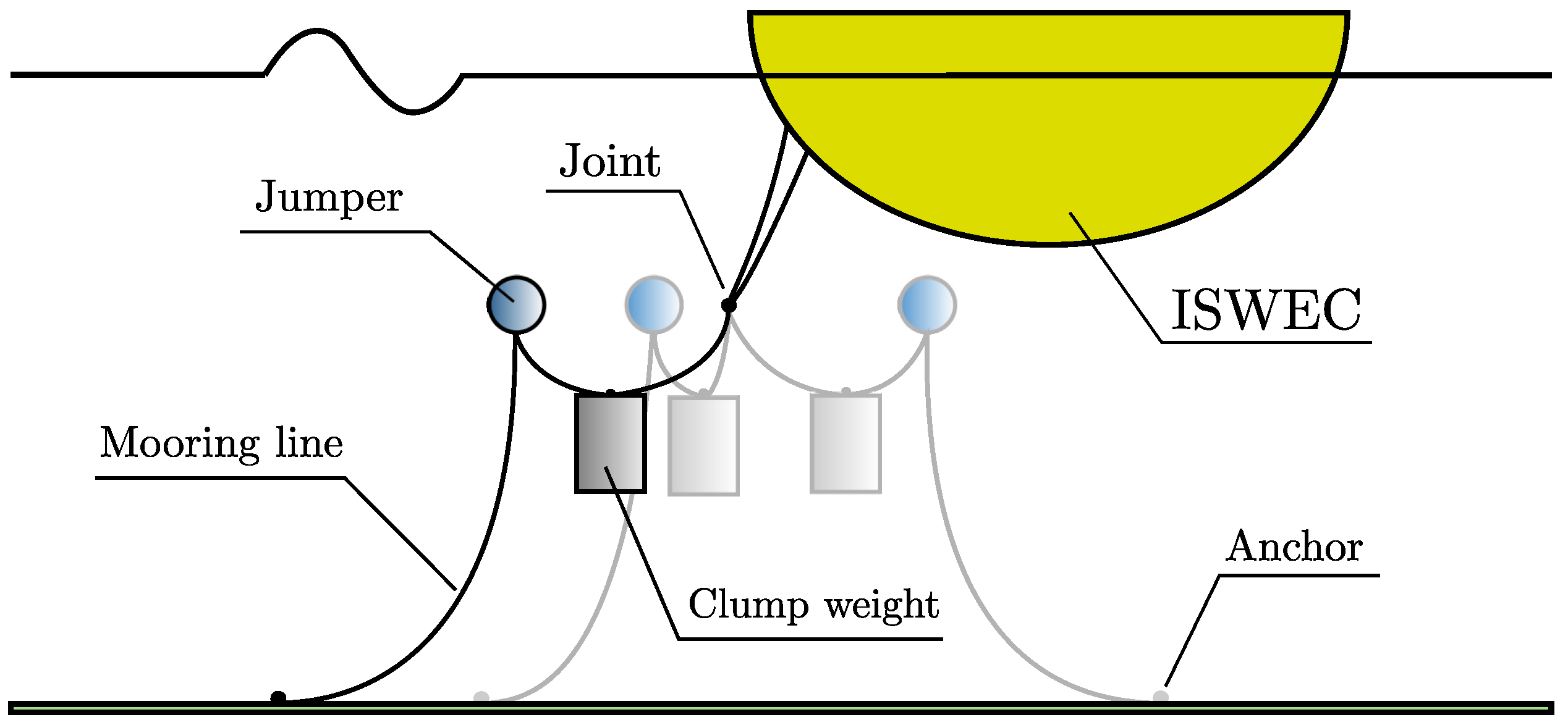
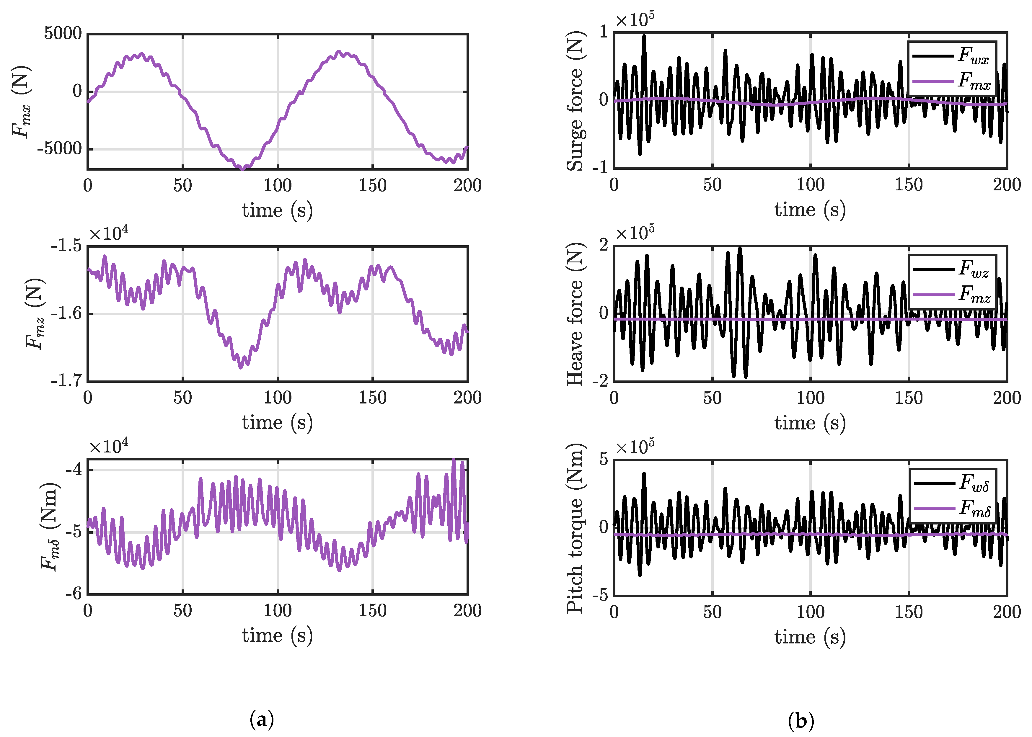
14) the mooring forces are considered as a unmodelled phenomena. In real applications, it would be difficult to directly measure the action of the moorings so they are included into the state vector as unknow states to be estimate. The ISWEC mooring system is designed to minimize the impact on the pitching motion of the device, appointed to the power conversion chain [31]. As demonstrated in Figure 7b, the mooring forces have a very slow dynamics such as the surge component and a constant load in heave and pitch directions compared to the WEF. In normal working conditions, snatch loads do not appear, and the mooring forces have mainly the behaviour as shown in Figure 7a. F m ( t ) is synthesised using the same method that was detailed for F w ( t ) , using a harmonic model to describe its behaviour. For the sake of simplicity, the mooring forces are modelled with only one frequency for each component representing their main spectral nature.
Under these assumptions the state vector X ( t ) is augmented including the estimation of F w ( t ) and F m ( t ) and the System (14) is re-written:
X ˙ a ( t ) = A a X a ( t ) + B a F g ( t ) Y ( t ) = C a X a ( t ) + D a F g ( t )
where X a ( t ) R n F is the augmented state vector defined as:
X a ( t ) = X ( t ) F ^ ( t ) F ^ ˙ ( t ) T
Here n F = n S + 2 n D ( n W + 1 ) is the augmented state vector dimension. F ^ R n D × ( n W + 1 ) is the unknown force to be estimated:
F ^ ( t ) = F ^ x ( t ) F ^ z ( t ) F ^ δ ( t ) T
The j-th compoenent of the estimated force is given by the WEF harmonics and the mooring force as follows:
F ^ j ( t ) = F ^ w j 1 ( t ) F ^ w j 2 ( t ) F ^ w j n W ( t ) F ^ m j ( t ) T
Therefore, the estimated F ^ w ( t ) is obtained by summing up all the harmonic contributions for each of its components:
F ^ w ( t ) = i = 1 n W F w x i ( t ) i = 1 n W F w z i ( t ) i = 1 n W F w δ i ( t ) T
The augmented matrices A a R n F × n F , B a R n F × n D , C a R m S × n F and D a R m S × n D are given by:
A a = 0 I 0 0 0 K M 1 B v M 1 C r M 1 M 1 N 0 0 B r A r 0 0 0 0 0 0 I 0 0 0 Ω 0 , B a = 0 M 1 0 0 0 C a = I 0 0 0 0 0 I 0 0 0 K M 1 B v M 1 C r M 1 M 1 N 0 , D a = 0 0 M 1
Again, I and 0 are identity and zero matrices according to the context. N R n D × ( n W + 1 ) is defined as:
N = I 1 , n W + 1 0 0 0 I 1 , n W + 1 0 0 0 I 1 , n W + 1
where I 1 , n W + 1 is a 1 × ( n W + 1 ) vector of ones. Ω R 3 ( n W + 1 ) × 3 ( n W + 1 ) is the diagonal matrix with the frequencies identified to approximate the unknown forces along the three DoFs:
Ω = Ω x 0 0 0 Ω z 0 0 0 Ω δ
In Equation (24), Ω x R ( n W + 1 ) × ( n W + 1 ) , Ω z R ( n W + 1 ) × ( n W + 1 ) and Ω δ R ( n W + 1 ) × ( n W + 1 ) are diagonal matrices containing the frequencies for unknown force components:
Ω j = d i a g ( ω w j ) 0 0 ω m j
where ω w j R n W stores the n W harmonics to model the WEF components. The number of frequencies in Ω , have to be chosen in order to have a compromise between the accuracy of the estimation for each excitation force component and the computational effort. The matrices (25) include a term at low frequency to represent the contribution of the mooring forces for each DoF.
Let us consider the following linear time-invariant stochastic discrete model representing the discrete-time version of the augmented System (17):
X ^ a d ( k + 1 ) = A a d X ^ a d ( k ) + B a d F g ( k ) + Γ w ( k ) Y d ( k ) = C a d X ^ a d ( k ) + D a d F g ( k ) + v ( k ) w ( k ) N ( 0 , Q ) v ( k ) N ( 0 , R )
where X ^ a d ( k ) represents the system estimated states, F g ( k ) is the known input and Y d ( k ) contains the measurements of the system dynamics. w ( k ) and v ( k ) are zero mean white noise sequences with known covariance, uncorrelated with each other and with the initial state of the system. A a d , B a d , C a d and D a d stand for the discretised versions of the matrices A a , B a , C a and D a . Γ is the weighting matrix for the process disturbances. Q and R are the covariance matrices of the process and measurements noise. The KF algorithm performs the estimation in the form of a feedback control: the filter estimates the process state at some time and then obtains feedback in the form of (noisy) measurements. As such, the equations for the KF fall into two groups: time-update equations and measurement-update equations [43]:
Time Update:
P ( k ) = A a d P ( k 1 ) A a d T + Γ Q Γ T X ^ a ( k ) = A a d X ^ a ( k 1 ) + B a d F g ( k 1 )
Measurement Update:
K ( k ) = P k C T C a d P ( k ) C a d T + R 1 P ( k ) = I + K ( k ) C a d P ( k ) X ^ a d ( k ) = X ^ a d ( k ) + K ( k ) Y ( k ) C a d X ^ a d ( k ) D a d F g ( k )
The time update equations can also be thought of as predictor equations, while the measurement update equations can be thought of as corrector equations. In this framework, the KF algorithm can be implemented to estimate the unknown WEF vector F ^ w ( k ) by measured system dynamics Y d ( k ) and known input F g ( k ) at any instant k.

4. Wave Excitation Force Estimation with Neural Network

Despite its simplicity and efficacy, the KF filter observer may suffer from several drawbacks: the non-linear effects emerging in sever sea-states conditions as well as the reliabiliy of the WEC model could negatively affect the estimation performances. For example, the slack-mooring of the ISWEC is modelled with a quasi-static approach (developed in-house). The main advantage consists in reducing the computational burden of the simulation at the expense of model accuracy. More accurate mooring models are presented in [44] considering two dynamic lumped-mass approaches (the open source MoorDyn [45] and the commercial OrcaFlex 11.0e [46]) where mooring actions are resolved coupling both the hydrodynamics and gyroscope model of the WEC in the MoorDyn and Orcaflex enviorments. When the system model is not reducible to a series of analytical equations or, even more, is based only on observed data the implementation KF model is not trivial. This argument can be extended to any other complex aspect of WEC modelling that cannot be analytically formulated with acceptable accuracy. In this context, artifical NNs represents powerful tools to map the non-linear relations from sets of input-output data. In NN models the parameters are tuned to fit the input-output data, without reference to the physical background and no information about the model architecture.
In general mathematical terms, WEFs acting on the ISWEC can be expressed as a non-linear function f ( ) of the system known inputs and measurements as follows [14]:
F ^ w ( k ) = f ( F g ( k ) , , F g ( k k N + 1 ) , Y d ( k ) , , Y d ( k k N + 1 ) )
Equation (29) shows that the estimation of the WEF at instant k is, at least in principle, addressed combining a series of known system inputs and measurements collected from discrete time k k N + 1 to k where k N represents the delay steps of the available data. More in detail, the WEF could be obtained from the set of WEC motion measurements from the ISWEC on-board sensors and the gyroscopic reaction. In [14] the same approach is considered including the measures provided by the IMU and encoders mounted on the ISWEC adding the velocity z ˙ d ( k ) and position z d ( k ) obtained by numerical integration of the acceleration z ¨ d ( k ) . These two inputs were included to improve the estimation accuracy. However, this measurements framework does not consider the effect of the sensor noise: in practice, accelerometer signals are often very noisy, hence velocity and position integration from acceleration are likely to be unreliable, resulting in unreliable estimations in practice. In this work, the NN is evaluated for all the configurations of 
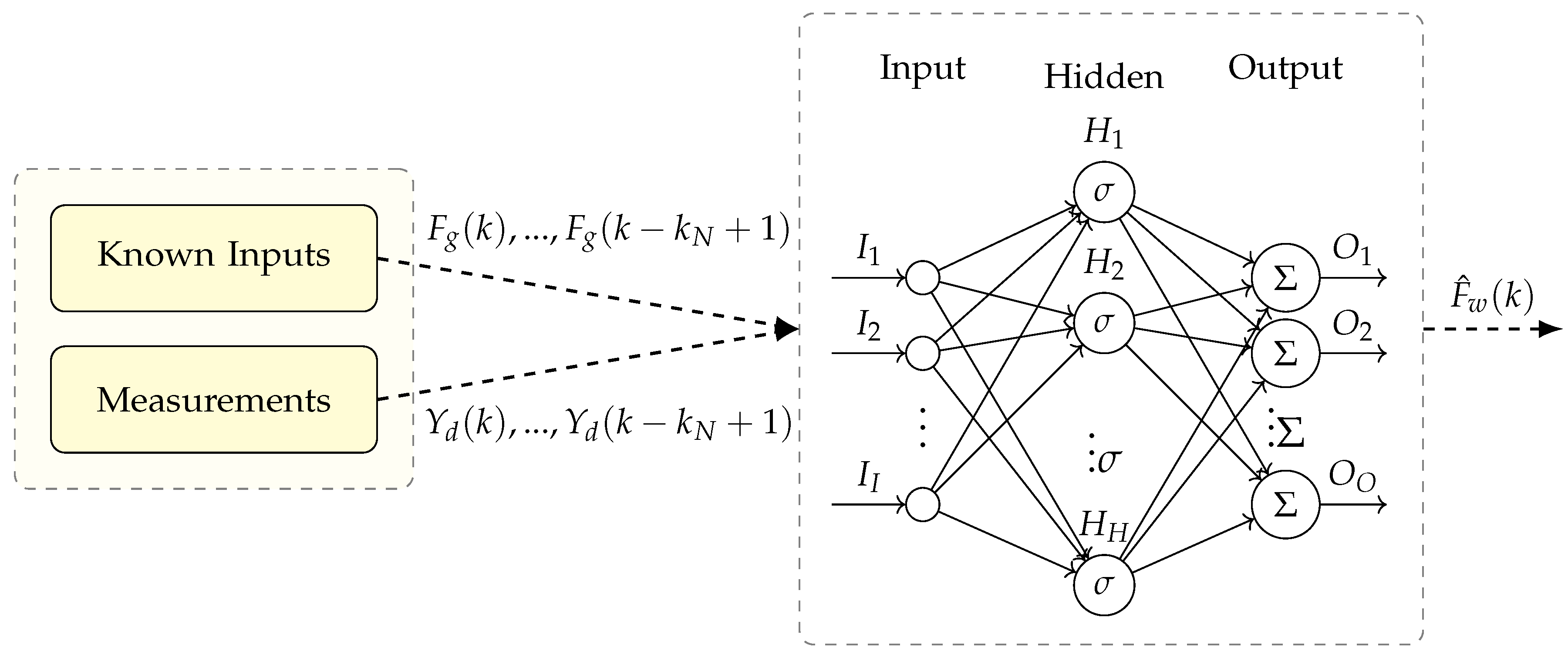
Table 2 and the sensitiveness and roubustness analysis is extended to all the wave domain of the installation site. The input-output architecture of the NN is shown in Figure 8. The feedforward NN is composed of linked neurons arranged in three layers. The input layer collects a set of inputs I I multiplying them by a set of weights, assigned to the data on the basis of their relative importance to other inputs. The hidden neurons apply a non-linear activation function σ to the weighted sum of their inputs. Then, the outputs of each hidden neuron are linearly combined by the output functions Σ to produce the network outputs O O . The use of delays in the input variables is considered to increase the reliability of the estimate. For a generic dynamic system, one way to consider its dynamic behaviour using static neurons is to employ past values of the inputs [47], resulting in good performances in term of estimation accuracy and robustness to different wave conditions as demonstrated in [14].

5. Kalman Filter and Neural Network Tuning

The matrix Ω containing the frequencies to model the WEFs as well as Q and R are tuned for the system under study. A sensitivity analysis has been performed to tune the number of frequencies. Then, through an iterative process the diagonal coefficients of Q and R are identified in order to have the best estimation performances for each measurement framework considered. Numerical experiments are conduced considering the four wave profiles of Table 1. The estimation performances are valuated considering the Goodness-of-Fit ( G o F ) proposed by [48]:
G o F j = 1 k = 1 T s F w j ( k ) F ^ w j ( k ) 2 k = 1 T s F w j ( k ) 2
In Equation (30), F w j ( k ) and F ^ w j ( k ) are the true and estimated WEF for the j-th DoF at discrete time instant k, respectively. T s is the total number of samples.

5.1. Kalman Filter Parameters

For the presented case, 1, 3, 6 and 9 frequencies are tested in order to find a compromise between the accuracy of the estimation process and the KF complexity. The interval is chosen between period 3 s and period 9 s, linearly spaced. Each point refers to the mean of each G o F j obtained from four tuning sea-states. The mooring components are modelled with only one period: 100 s for F m x ( t ) and 2000 s for F m z ( t ) and F m δ ( t ) , considered as low frequency contributions (Figure 7). The FM framework has been considered for this tuning process. Table 3 sets out the results obtained from each tuning wave gruped in respect to the number of frequencies n W .
Increasing the number of harmonics from n W = 1 to n W = 3 leads to a significant improvement of all G o F . On average, an advance of 0.162 is obtained for G o F x , 0.138 for G o F z and 0.228 for G o F δ . Passing from n W = 3 to n W = 6 shows a slight increase of G o F x and G o F z , enchancing the quality of the F ^ w x ( t ) and F ^ w z ( t ) estimation of 0.011 and 0.021, respectively. Further enlarge of n W results in a minimal or null upgrade of any G o F . In this regard, n W = 6 is considered a good trade-off between accuracy and complexity of the observer.
For what concerns the covariance matrices, repeated simulations are conduced to tune the diagonal elements of Q and R for each mesurement framework. They are chosen to guarantee an accurate estimation of the unknown states without amplifying the noise level. 
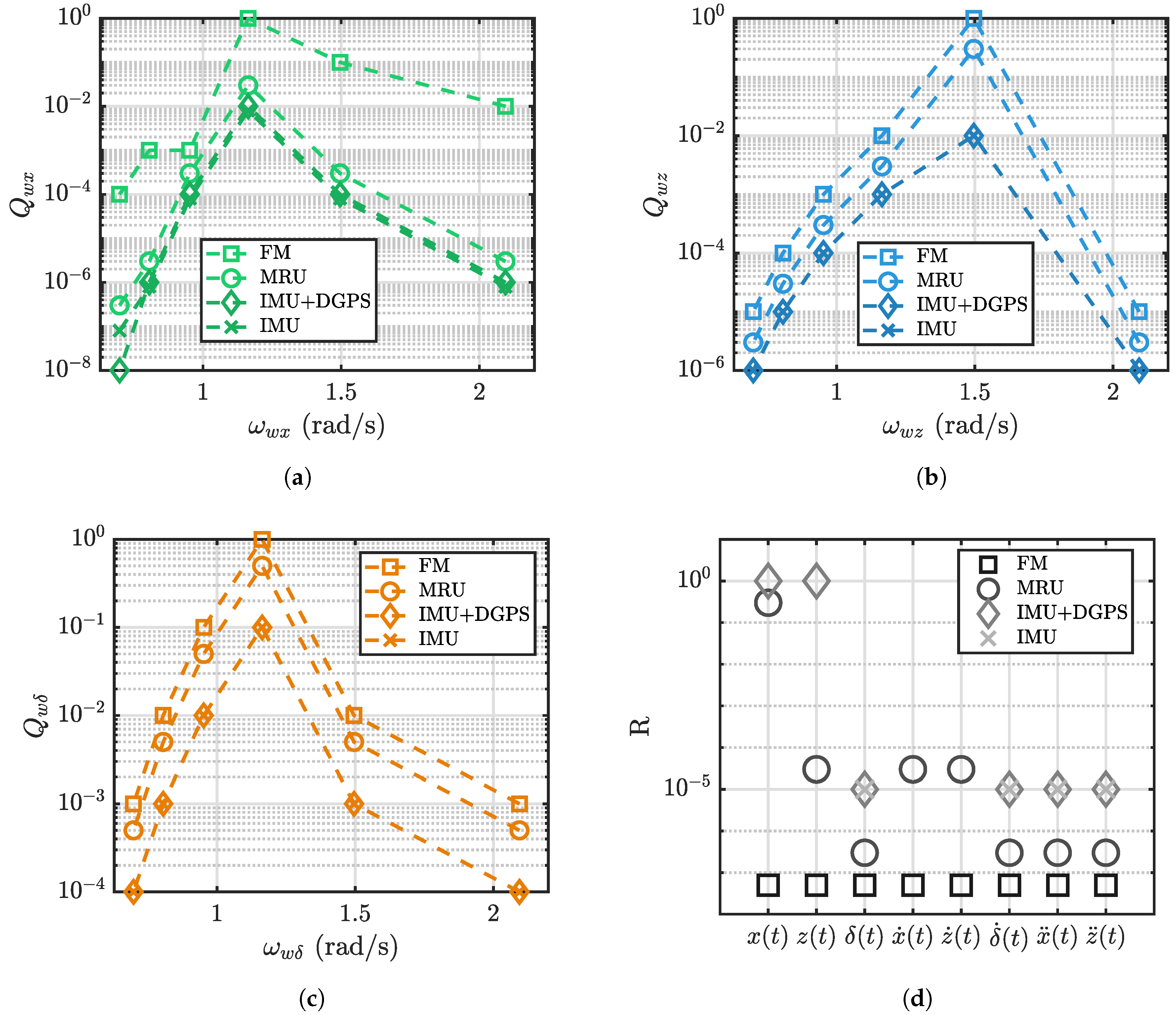
Figure 9a–c compare the Q coeffcients relative to the WEF components for each measurement framework. From the chart, it can be seen that the Q coeffcients are reduced as the magnitude of the noise increases and are tuned in respect to the energy content of the WEF. In this way, the most relevant frequency components are amplified more than the others, resulting in a more accurate estimation. Figure 9d provides the R coefficients, balanced in order to penalize the most inaccurate measurements (e.g., DGPS positions) giving less importance to the related signals. Data indicate that the R coefficients grow as the noise magnitudes increase. Missing markers mean that the measurements are not available for that framework.

5.2. Neural Network Parameters

The NN training aims to obtain the weights and bias of the network evaluating the sensitivity of the model to both the delay steps k N and neurons n N . The four wave profiles of Table 1 are used to obtain the training data for each measurement framework. The time-series of the WEFs are concatenated to generate a long training set applied to the ISWEC numerical model obtaining the WEC motion measurements. Then, all the time-series are normalized in the [ 1 , 1 ] range to avoid problems due to different magnitude between input-output signals. Since the system is non-linear, the data normalization could negatively affect the trainign process if, for example, saturations of the PTO appear. To avoid saturations, the training data are chosen to cover the operating range of the ISWEC. However, in sever sea-states the WEC motion could overcome the normalization range causing estimation errors but, in such extreme conditions, the WEC is shut-down for safety purposes and no control is applied. In order to address over-fitting problem the data are randomly divided into three parts: 50% for training purposes, 30% for validation and 20% for performance evaluation. The performance function is the Mean Squared Error (MSE) normalized between −1 and 1, ensuring that the relative accuracy of output elements of different magnitude are treated as equally important. Then, 1, 3, 5, and 7 delay steps are tested while the number of neurons is fixed to 10; 5, 10, 15 and 20 neurons are evaluated with 3 delay steps. Specific tuning processes are applied for each framework with the same number of delay steps and neurons, considering noisy signals. The FM framework has been considered for tuning the network hyperparameters.
The sensitivity analysis on the delay steps is reported in Table 4. The mean value of each G o F reveals that increasing the number of delay steps from k N = 1 to k N = 3 results in a revelant increase of estimation accuracy, expecially for the G o F δ that passes from 0.880 to 0.977. A similar behaviour is obtained for the G o F x , where the mean estimation performance grows of 0.053 points. On the other hand, no relevant improvements are obtained for the G o F z as well as for the other DoFs employing 5 and 7 delay steps. In this regard, 3 unit delays are chosen for the NN architecture.
Table 5 reports the estimation results obtained for different values of neurons. 10 neurons represents the best choise ensuring the good estimation performances with acceptable network complexity. Surprisingly, increasing the number of neurons over 10 leads to a slight degradation of performances, suggesting that the learning algorithm is not able to converge properly during the learning process over-fitting noisy data.

6. Numerical Results and Discussions

In this section, several results are carried out for a comprehensive analysis of the KF and NN performances. An exhaustive evaluation in different wave conditions as well as a robustness evaluation to different measurements and plant inaccuracies is provided. Both the KF and NN are tested and compared extending the wave domain to the 35 waves represented in Figure 4. Each G o F j is weighted on the annual energy of the specific site in analysis:
G o F ¯ j = v = 1 V G o F j ( v ) E ( v ) v = 1 V E ( v )
In Equation (31), E ( v ) is the annual energy associated to v-th wave and V the total number of waves considered. Then, the percentage difference between the KF and NN results is defined as follows:
Δ G o F ¯ j = G o F ¯ j | N N G o F ¯ j | K F G o F ¯ j | K F 100
where G o F ¯ j | K F and G o F ¯ j | N N are the weighted G o F obtained with KF and NN, respectively.

6.1. Influence of the Measurement Framework

The available measurements and their accuracy play an important role in the estimation process. The main question concerns the influence of the available signals and how missing data can affect the estimation performances. The three measurement configurations MRU, IMU+DGPS and IMU are compared considering noisless data. In order to improve readability, some of the bulky figures are placed in the Appendix A.
Focusing on the KF results, Figure A1 is quite revealing in several ways. Overrall, maximum estiamtion performances are found near the tuning waves (marked with black squares) except for the G o F z provided by the IMU framework. In particular, best performances are achieved in the range [ 4 , 8 ] seconds as the period interval is chosen between 3 s and 9 s. In a practical setup, an accurate analysis the dominant periods is crucial to achieve the best performances from the KF. Moreover, promising results are obtained in all the sea-states considered, suggesting a good versatility of the observer where the system is not tuned. The accuracy is almost the same for the force components in surge and pitch directions. Despite the configuration IMU+DGPS does not provide the x ˙ ( t ) signal, the IMU+DGPS equipment is able to estimate the F ^ w x ( t ) component with the same accuracy as the MRU one. The same argument can be applied considering the IMU results. In spite of the IMU does not provide both x ( t ) and x ˙ ( t ) , its accuracy of the pitch force estimation equals the MRU and IMU+DGPS one. Since surge and pitch DoFs are coupled due to the device geometry, the surge force can be succesfully estimated from the pitching motion of the device (available in all the frameworks). Morevoer, the effect of the damping is negligible and the hydrostatic stiffness is null in the surge direction, not affecting the estimate of F ^ w x ( t ) . For what concern the heave component, there is a significant difference between the G o F z of the IMU and the other two frameworks. The absence of both z ( t ) and z ˙ ( t ) leads a decrease of performances since, as illustrated in Figure 10, the KF is not able to estimate correctly the position z ( t ) resulting in a loss of estimation accuracy.
Considering the NN, Figure A2 demonstrates that the NN performance is maximized with a MRU measurement framework and near the tuning waves. In agreement with the KF, removing the absolute velocities x ˙ ( t ) and z ˙ ( t ) leads to a minimal decrease in estimation accuracy for all the DoFs. This finding is expected for both surge and pitch DoFs since the measurements that influence the F ^ w x ( t ) and F ^ w δ ( t ) estimation ( δ ( t ) , δ ˙ ( t ) and x ¨ ( t ) ) are provided both in MRU and IMU+DGPS configurations. The lack of performance increase for the IMU framework, especially for the heave DoF where the goodness of estimation significantly reduces for all the waves, suggesting that the NN is not able to obtain an appropriate fit of the F w z ( t ) if a full measurement framework is not provided. On the other hand, δ ( t ) , δ ˙ ( t ) and x ¨ ( t ) are adequate to succesfully estimate the F ^ w x ( t ) and F ^ w δ ( t ) components, as demonstrated for the KF observer.

6.2. Sensor Noise Effect

Once the influence of the available measurements is evaluated, realistic data are applied both to the KF and NN to assess the effect of the sensor disturbances. Starting with the KF observer, Figure A3 highlights that the MRU framework gives almost the same precision compared to the noiseless case, especially for the surge and pitch excitation forces. MRU units are affected by minimal disturbances and offer an accurate measures of angular rates, orientations, accelerations, velocities and positions. The use of IMU+DGPS intruduces higher estimation errors due to the increase of noise. In particular, the positions are the most polluted due to a noise RMS equal to 0.5 m (Table 2) as depicted in Figure 11. The errors introduced by the DGPS are the same order of manitude of the heave motion z ( t ) providing a significant decrease in performance of the F ^ w z ( t ) estimation. The performances of the IMU framework almost equalize the IMU+DGPS one for all the DoF. As demonstrated for the noiseless case, it is apparent that removing the DPGS noisy measurements does not affect the quality of the estimation. Having a good quality in δ ( t ) , δ ˙ ( t ) and x ¨ ( t ) acquisitions allows to effectively handle the estimation of the coupled DoF since they mutually influence each other. For what concern the G o F z value, the error introduced by the DGPS forces to increase R coefficient associated to z ( t ) to such an extent that its measurements are not taken into account. This demonstrate why IMU+DGPS and IMU have similar performances for the heave component.
As shown in Figure A4, the introduction of noisy measurements negatively affects the estimation accuracy of the NN, expecially for the heave DoF. A relevant degradation of performance is shown for the IMU+DGPS and IMU framework estimating the wave exctitation force along the heave direction. As demostrated in Figure 11, the heave motion provided by the DGPS is heavily polluted by sensor noise making the NN unable to estimate the heave component with acceptable accuracy. In this context, the KF implementing the IMU+DGPS or IMU unit exploits the heave acceleration to estimate the F ^ w z ( t ) component with almost double precision than the NN.

6.3. Sensitivity to Plant Variations

In order to evaluate the effectiveness of KF and NN, the architectures are tested considering a typical case may happen in practice: variation of the physical properties of the floater. In fact, the WEC model may differ from its built version passing from the theoretical design to its construction in the shipyard and, even more, during its life cycle due to wear and biofouling. A further analysis is performed, testing the behavior of the frameworks modifying the mass matrix M and stiffness matrix K. An iterative method is proposed varying both the mass and stiffness matrix in respect to the nominal value as follows:
M c = M ¯ M K c = K ¯ K
where M ¯ and K ¯ are the correction coefficients and M c and K c the corrected values. M ¯ and K ¯ span from 0.85 to 1.15. At this point, the performances of the KF are shown in Figure 12 in term of G o F ¯ . The decrease of performances is limited for the surge component. The variation of the mass matrix results in a decay of almost 0.1 of G o F ¯ x for all the measurement frameworks. The stiffness matrix does not influence the estimation of the F ^ w x ( t ) since the hydrostatic stiffness is null in the x direction. In this regard, no variation of G o F ¯ x is detected in Figure 12d. The degradation of performance is quite sensitive to the mass and the stiffness variation for heave and pitch DoFs. As to the mass matrix, the G o F ¯ d e l t a in Figure 12c shows an higher decrease since pitch-surge modes are coupled and the estimation is influenced both by the diagonal and off-diagonal terms of M; as demonstrated in [14], the pitch force estimation is more influenced than the heave one because more terms of M are modified at once. The K variation results in a decay of almost 0.2 in both G o F ¯ z and G o F ¯ δ for all the measurement frameworks as depicted in Figure 12e,f.
Figure 13 illustrates the influence of M ¯ and K ¯ for the NN framework.
A mean decrease of 0.1 is shown for all the measurement frameworks in presence of mass matrix variations, except for a high reduction of G o F δ with the MRU configuration. The NN is merely a non-linear function that maps a serie of input-output arguments regardless of any phisical background. The training algorithm considers all the measurements available from the MRU to train the NN and a variation of the mass matrix influences all the measurements data provided to the network leading to a lower estimation accuracy. On the other hand, IMU+DGPS and IMU consider few measurements and appear to be less sensitive to plant variations. In particular, the G o F δ suffers of a decrease up to 0.3 for a K ¯ of 0.85 and almost 0.25 for a K ¯ equal to 1.15, suggesting again that the MRU framework is less robust in presence of plant variations with the NN model. Likewise, a stiffness matrix variation negatively affects the estimation accuracy of F ^ w x despite its estimation is influenced only by δ ( t ) , δ ˙ ( t ) and x ¨ ( t ) acquisitions as demostrated for the KF observer.

6.4. Comparison and Summary

The weighted GoFs and percentage differences of the KF and NN results are summarized in Table 6. The apex * means that no disturbances are considered. Starting from noiseless results, the G o F x ¯ and G o F δ ¯ values confirm that the measurements of an IMU * unit are sufficient to estimate the surge and pitch components with acceptable accuracy. In detail, excluding absolute displacements and velocity measurements the G o F ¯ x | K F decreases from 0.910 to 0.893, the G o F ¯ δ | K F from 0.901 to 0.899, the G o F ¯ x | N N from 0.951 to 0.931 and the G o F ¯ δ | K F from 0.961 to 0.940. G o F ¯ z follows the same behaviour, especially from the IMU+DGPS* to IMU* framework where a decrease of 0.229 and 0.397 appear for the KF and NN, respectively. Comparing the two techniques, the performance of the NN model surpasses the KF perfromance for surge and pitch DoFs, especially for the pitch DoF where an increment of 6.65%, 6.31% and 5.73% is achieved. However, the estimation of the heave force is not reliable with the NN, where a difference of −28.5% is obtained. Interestingly, the NN is able to handle noisy data better than the KF for both surge and pitch DoF, except for the IMU case. Specifically, a minimal difference of 2.73% is obtained with the IMU framework in surge direction. The NN always overcomes the G o F ¯ δ of the KF with a peak of 6.70% with a MRU unit. On the other hand, poor performances are carried out for the heave DoF with the NN, obtaining a weighted GoF almost equal to 0.3 for both IMU+DGPS and IMU.
Surprisingly, the sensitivity of the KF in presence of plant inaccuracies is evident compared to the NN. In particular, Figure 14 highlight a relevant decrease in performance for F ^ w δ ( t ) estimation with a M ¯ and K ¯ variation when the KF is employed (IMU framework). Using the KF, the results show a decrease of performances up to 0.18 points varying M ¯ and 0.20 varying K ¯ . In contrast, the NN guarantee a weighted G o F ¯ δ always greater than 0.77 suggesting low sensitivity when plant variations appear. In all likelihood, the sensitivity of the KF could be diminished tuning the matrix Q in order to give less importance to the model in favor of measurements. However, more research on this topic needs to be undertaken before the association between Q and KF sensitivity is more clearly understood.
The real ISWEC system is equipped with the MTi unit presented in Section 2.2.7. Unlike the MRU, the IMU unit does not provide positioning data and the measurement noise are one order of magnitude higher than the MRU ones. Although more information are available with the MRU, the IMU framework provide acceptable accuracy for both surge and pitch wave forces, directly involved in the power extraction. In detail, in case of noisy measurements and KF observer, the weighted accuracy approaches 0.88 and 0.82 for G o F ¯ x and G o F ¯ δ , respectively; with the NN the accuracy is about 0.85 and 0.84 for G o F ¯ x and G o F ¯ δ , respectively. Moreover, the MRU units are (usually) one order of magnitude more expensive than the IMU ones, and the precision provided does not justify the little increase of performances, expecially in the KF case. Despite the low performances obtained for the WEF in heave direction (not directly involted in the power extraction), the IMU sensor is considered reliable for the estimation.

7. Conclusions

The purpose of this work is to estimate the WEFs of a non-linear WEC employing a KF observer and a NN model. This study proposes a methodology for tuning both estimators and compares them for a wide range of sea-states in presence of noise disturbances and plant variations. Four different measurement frameworks are proposed, one ideal (full measurements available without noise) and three real frameworks composed by three different sensors commercially available. The main aim is to assess the estimation performances in term of GoF for different sensor equipments in all the operating conditions of the ISWEC device. The non-linear 3-DoF model of the ISWEC is considered as the plant of reference. A linear 3-DoF hydrodynamic model is used in the KF assuming linear wave theory and linear viscous damping along the pitch DoF. Moreover, the filter model assumes no viscous damping in both surge and heave directions and the mooring forces are considered as an unknow state to be estimated. The key of the KF is to approximate the expression of the WEFs as a linear superposition of finite harmonic components with variable amplitudes and fixed frequencies. Hence, it is possible to include the excitation forces into the state vector of the system model and perform an unknown state estimation. This method restricts the bandwidth of the estimated disturbance as it can only estimate at the specified discrete frequencies. This makes it more robust to other external disturbances such as unmodelled hydrodynamic forces outside from the frequency range considered. The feedforeward NN is designed according to the hydrodynamic equation of the ISWEC. The WEFs are expressed as a function of the system dynamics at current and past time instants taking into account the dynamic memory of the plant using static neurons with no feedback data.
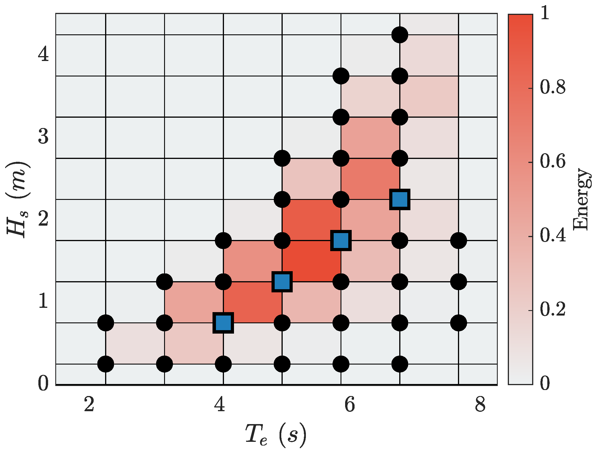
First, the KF parameters are tuned according to the frequency range, stating the WEF frequencies and the mooring frequencies. The wave energy matrix of the sea-site of interest has been considered to identify the principal wave periods of the incoming sea-states to decouple them from the mooring actions. Moreover, according to the noise magnitudes of the sensors, matrices Q and 
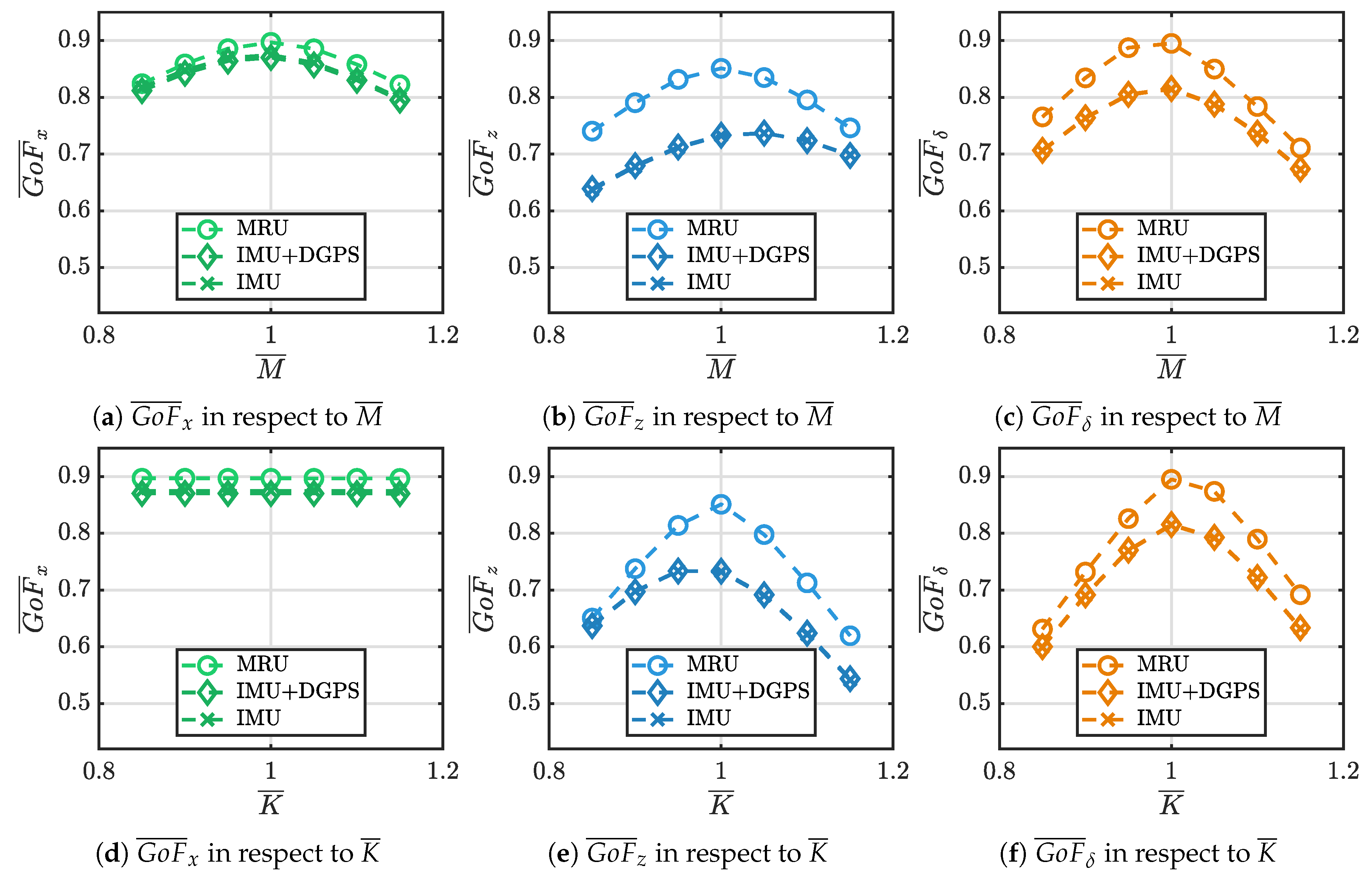
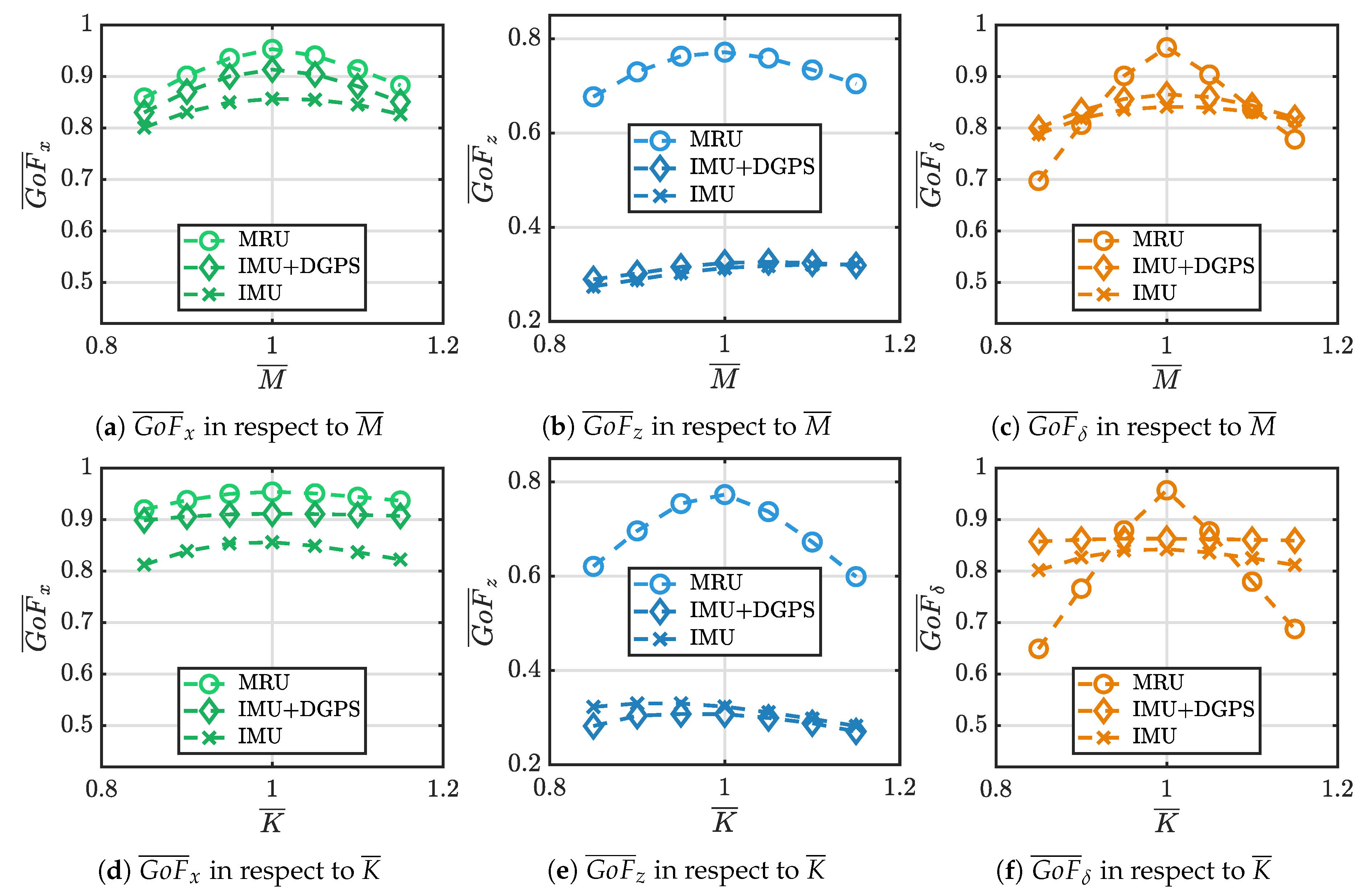
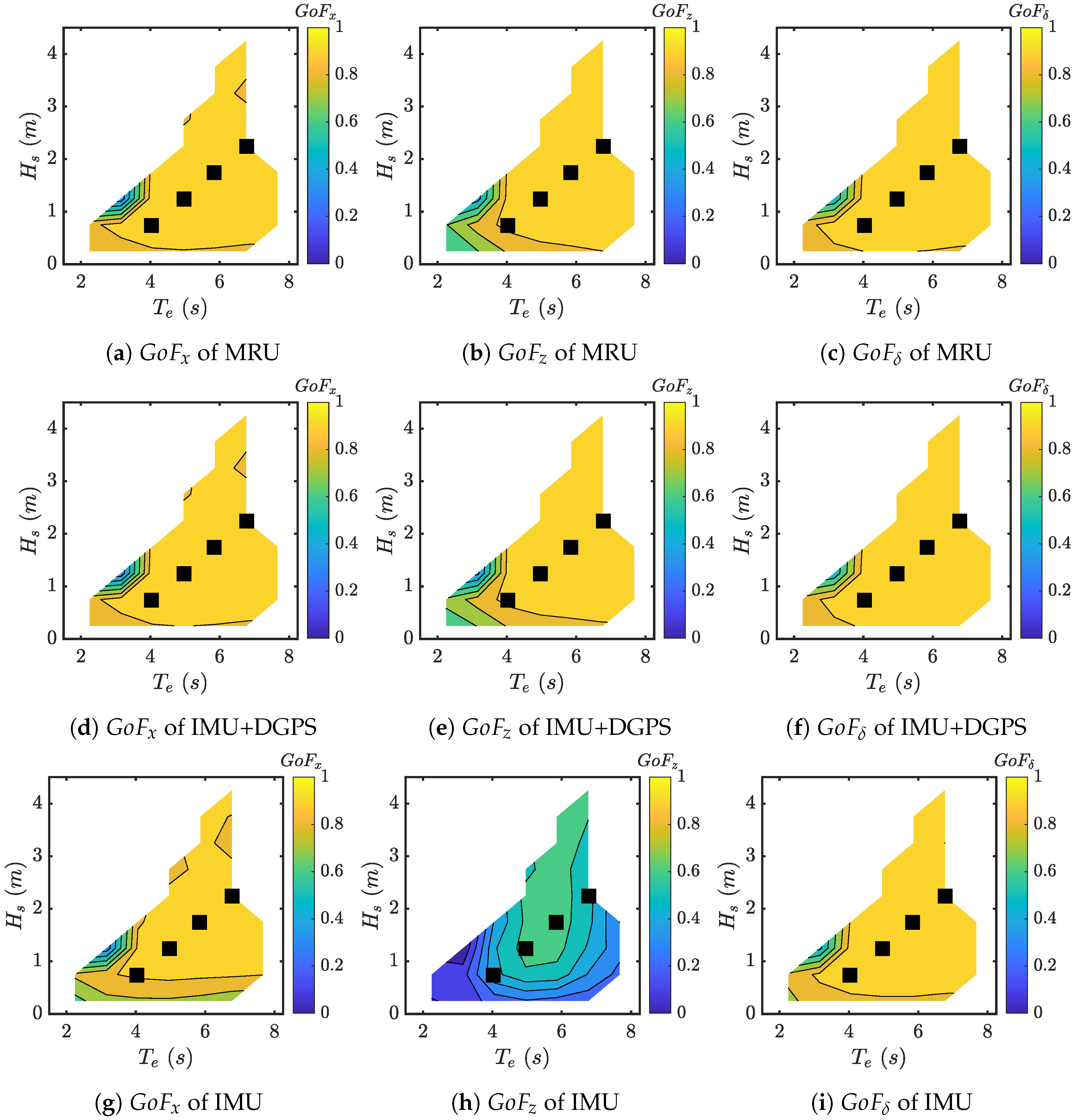
R have been balanced to obtain the best GoF from each measurement framework. The NN has been tuned with the same intent, chosing both delay steps and number of neurons guaranteeing the best compromise between network complexity and estimation accuracy. Second, numerical simulations are performed to investigate the influence of the measurement framework and sensors accuracy. Overrall, it is demonstrated that the 3-DoF KF performs well when applied to a non-linear WEC model. The KF shows best performances with the MRU* and IMU+DGPS* frameworks, expecially in surge and pitch directions where a G o F ¯ x and G o F ¯ δ greater than 0.9 are guaranteed. The IMU* framework gives the worst performances along the heave direction performing a G o F ¯ z 
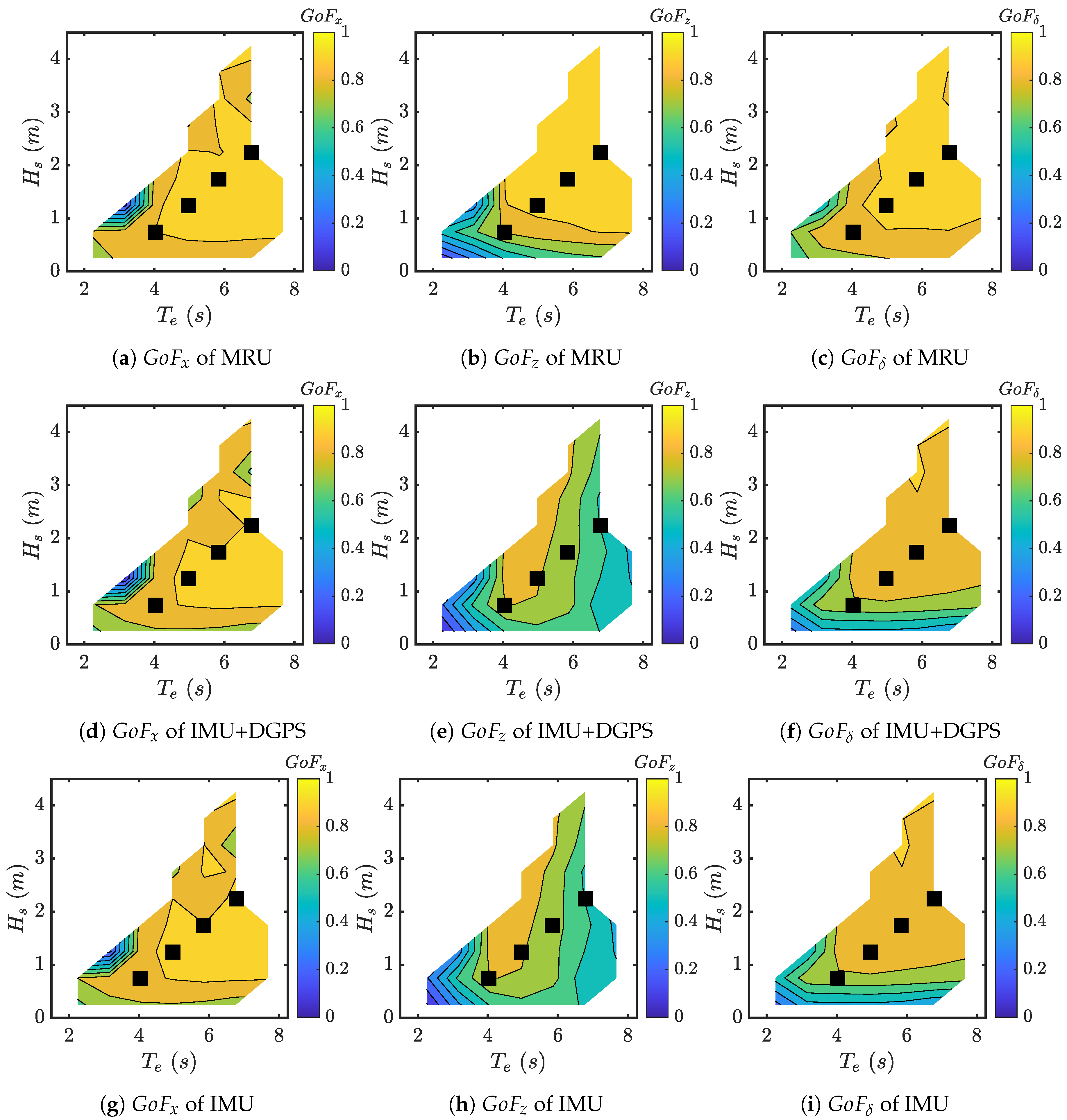
almost equal to 0.75. The same argument applies for the NN, where the estimation performances are maximized in surge and pitch. Adding noisy measurements results in an acceptable decrease of accuracy for G o F ¯ x and G o F ¯ δ . In detail, the comparison shows that the estimation accuracies of NN and KF are approximately the same and a
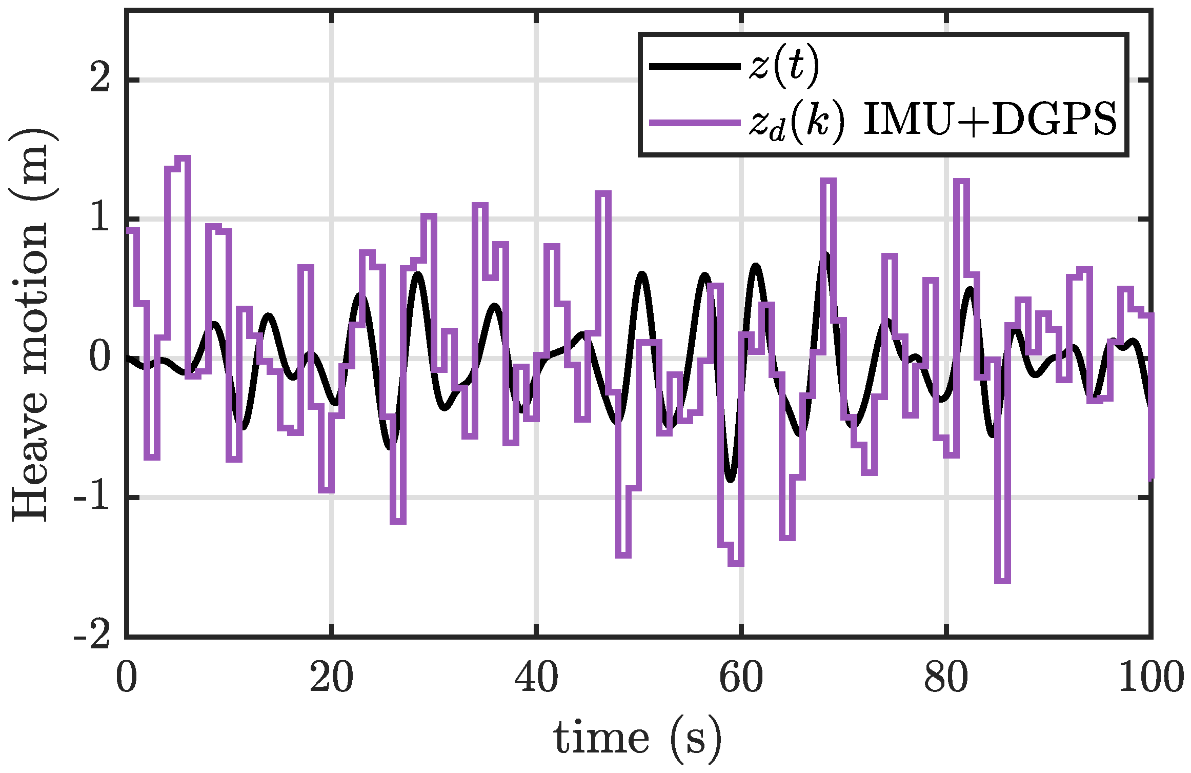
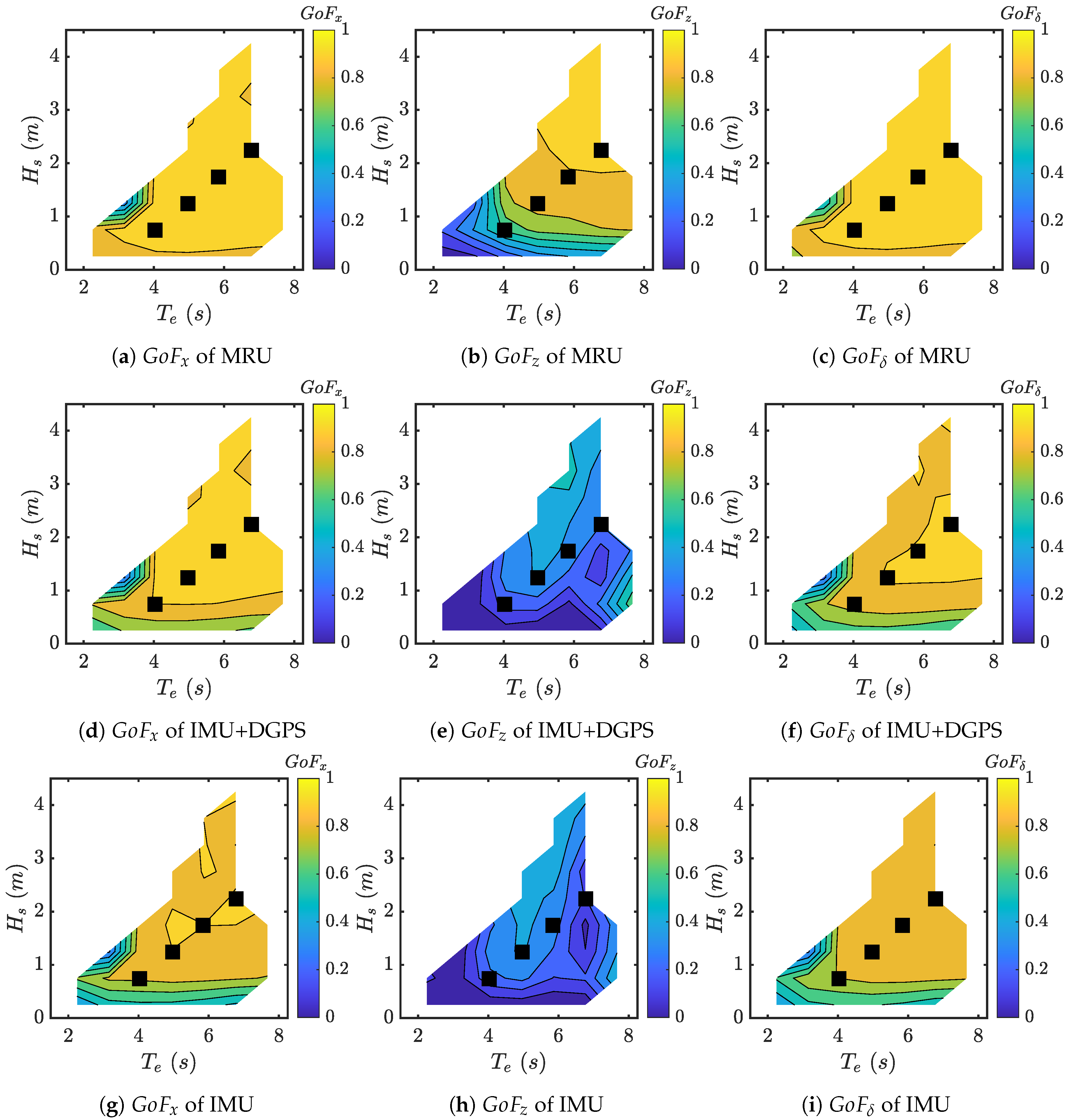
 G o F ¯ x and G o F ¯ δ 
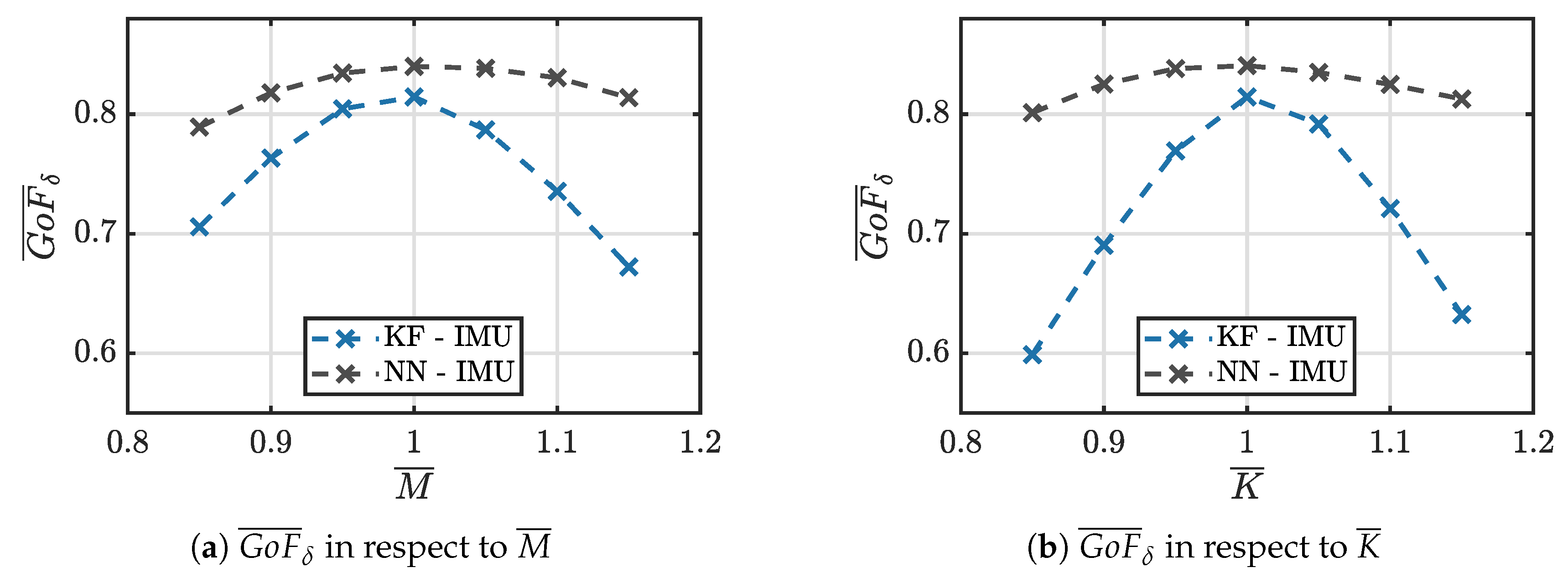
greater than 0.83 is obtained. However, both the KF and NN are considered not reliable for the WEF estimation along the heave DoF if DGPS and IMU are employed. Then, intersting results are obtained comparing the estimation performances under plant variations. Contrary to expectations, the KF is affected by plant variations more than the NN. Despite the KF can handle inaccuracies of the numerical model tuning on the Q matrix, the NN shows good performances when these inaccuracies become relevant. Further work is required to establish the underlying cause of this outcome, acting on the Q matrix to improve the mean performances of the KF observer.
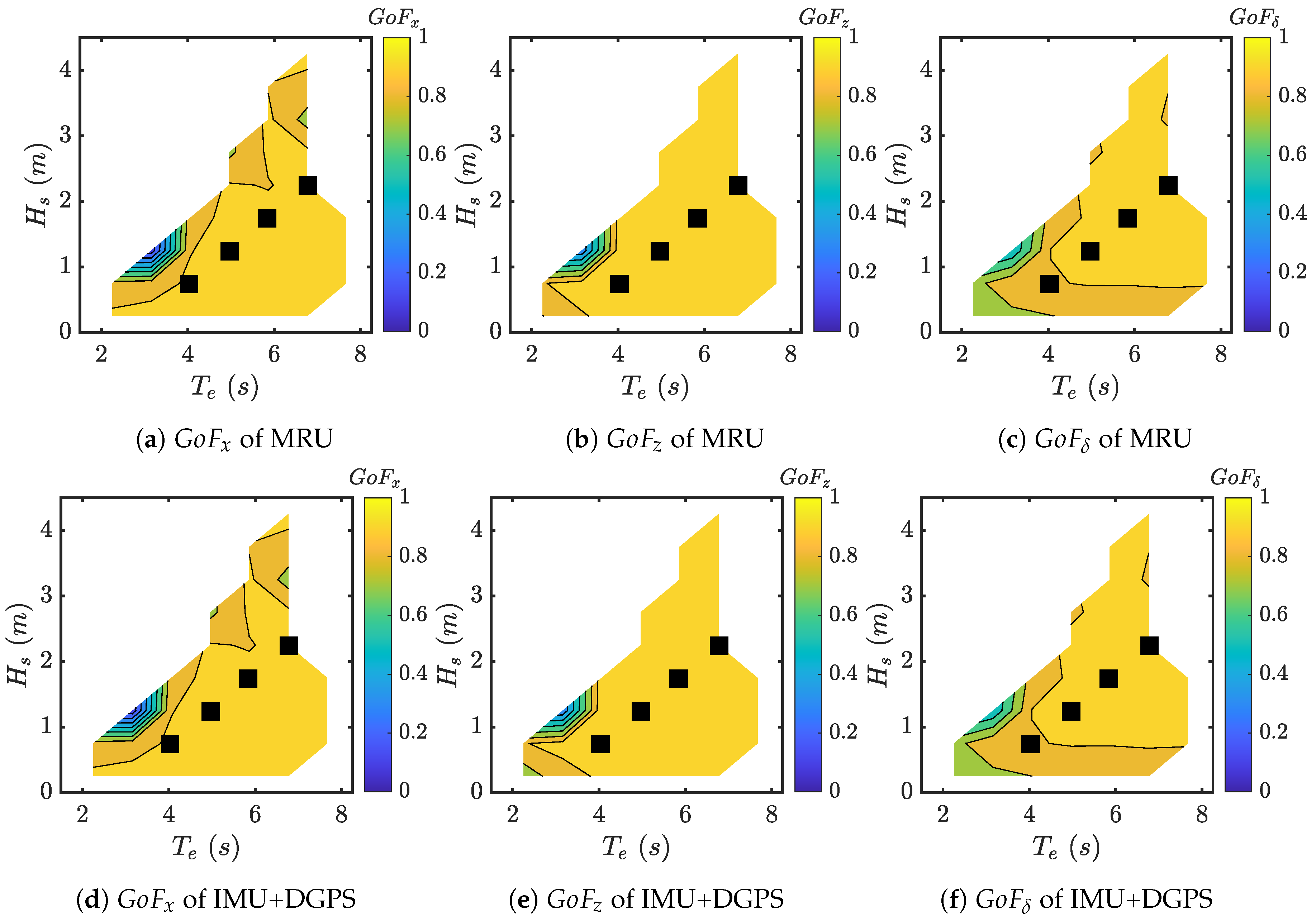
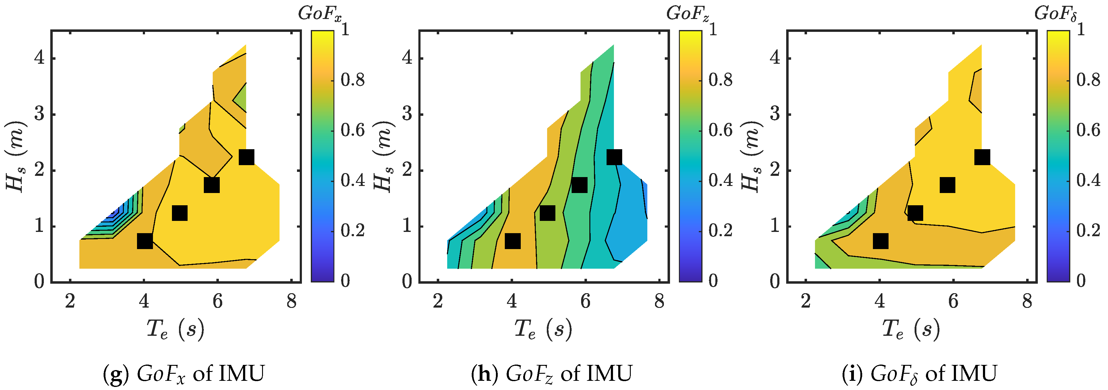
 Section 6.1, Section 6.2 and 
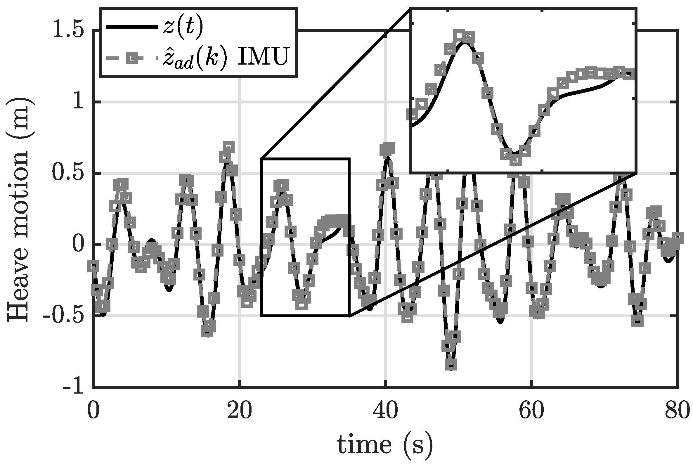
Section 6.3 demonstrated the good reliability of the IMU framework for the WEF estimation in surge and pitch directions for both KF and NN. However, it is evident how the estimation of the heave component is affected by the absence of the heave motion in the KF and both heave motion and velocity in NN. Despite this outcome, the use of the IMU unit is encourageed since the F ^ w z ( t ) is not directly involved in the power extraction of the ISWEC.
In conclusion, the main advantage of the model-based approach is that in presence of a real plant, it is possible to tune the observer on a small number of waves to obtain accurate estimation performances for a large number of sea states. The main strength of the KFHO is to consider only the frequency bandwidth specified; the knowlegde of the spectral properties of the signal to estimate allow to exclude all the undesired components and disturbance from the estimation (e.g., Mooring forces). On the other hand, a model-free non-linear approach should be more suitable to model complex hydrodynamic phenomena when their analytical expression are not available. Future work will approach the problem of the WEF estimation using more non-linear approaches (e.g., Recurrent Neural Networks and Extended Kalman Filter). The non-linear approach is expected to be more accurate in presence of strong non-linearity (e.g., PTO saturations and non-linear mooring models) in respect to a linear model-based observer. The aim will be elaborate on the estimation results between a model-based and model-free approach in term of estimation performances for a broad range of sea states. The best estimation approach will be used for the implementation of the MPC strategy on ISWEC.

Author Contributions

Conceptualization, M.B., A.H., S.A.S., P.D., G.B., G.M. and A.P.; methodology, M.B., A.H., S.A.S., P.D., G.B., G.M. and A.P.; software, M.B. and A.H.; validation, M.B., A.H., S.A.S. and P.D.; formal analysis, M.B., A.H., S.A.S., P.D. and G.B.; investigation, M.B. and A.H.; resources, G.B., G.M. and A.P.; data curation, M.B. and A.H.; writing—original draft preparation, M.B. and A.H.; writing—review and editing, M.B., A.H., S.A.S., P.D. and G.B.; visualization, M.B., A.H., S.A.S. and G.B.; supervision, G.M. and A.P.; project administration, G.M. and A.P.; funding acquisition, G.B. and G.M. All authors have read and agreed to the published version of the manuscript.

Funding

This research received no external funding.

Conflicts of Interest

The authors declare no conflict of interest.

Appendix A Figures

Appendix A.1. GoF with Noiseless Data and KF Observer

Figure A1. G o F results with noisless measurements for each measurement framework obtained with the KF. The first row refers to the MRU framework (ac), the second to the IMU+DGPS framework (df), the thrid to the IMU framework (gi).
Jmse 08 00825 g0a1aJmse 08 00825 g0a1b

Appendix A.2. GoF with Noiseless Data and NN Model

Figure A2. G o F results with noisless measurements for each measurement framework obtained with the NN. The first row refers to the MRU framework (ac), the second to the IMU+DGPS framework (df), the thrid to the IMU framework (bi).
Jmse 08 00825 g0a2

Appendix A.3. GoF with Noisy Data and KF Observer

Figure A3. G o F results with noisy measurements for each measurement framework obtained with the KF. The first row refers to the MRU framework (ac), the second to the IMU+DGPS framework (df), the thrid to the IMU framework (gi).
Jmse 08 00825 g0a3

Appendix A.4. GoF with Noisy Data and NN Model

Figure A4. G o F results with noisy measurements for each measurement framework obtained with the NN. The first row refers to the MRU framework (ac), the second to the IMU+DGPS framework (df), the thrid to the IMU framework (gi).
Jmse 08 00825 g0a4

References

  1. Faedo, N.; Olaya, S.; Ringwood, J.V. Optimal control, MPC and MPC-like algorithms for wave energy systems: An overview. IFAC J. Syst. Control 2017, 1, 37–56. [Google Scholar] [CrossRef] [Green Version]
  2. Pena-Sanchez, Y.; Windt, C.; Davidson, J.; Ringwood, J.V. A Critical Comparison of Excitation Force Estimators for Wave-Energy Devices. IEEE Trans. Control Syst. Technol. 2019, 1–13. [Google Scholar] [CrossRef]
  3. Ling, B.A.; Batten, B.A. Real Time Estimation and Prediction of Wave Excitation Forces on a Heaving Body. In Proceedings of the International Conference on Offshore Mechanics and Arctic Engineering, St. John’s, NL, Canada, 31 May–5 June 2015. [Google Scholar]
  4. Garcia-Abril, M.; Paparella, F.; Ringwood, J.V. Excitation force estimation and forecasting for wave energy applications. IFAC Pap. 2017, 50, 14692–14697. [Google Scholar] [CrossRef]
  5. Pena-Sanchez, Y.; Garcia-Abril, M.; Paparella, F.; Ringwood, J.V. Estimation and Forecasting of Excitation Force for Arrays of Wave Energy Devices. IEEE Trans. Sustain. Energy 2018, 9, 1672–1680. [Google Scholar] [CrossRef] [Green Version]
  6. Nguyen, H.N.; Tona, P. Wave Excitation Force Estimation for Wave Energy Converters of the Point-Absorber Type. IEEE Trans. Control Syst. Technol. 2018, 26, 2173–2181. [Google Scholar] [CrossRef] [Green Version]
  7. Abdelrahman, M.; Patton, R.; Guo, B.; Lan, J. Estimation of wave excitation force for wave energy converters. In Proceedings of the 2016 3rd Conference on Control and Fault-Tolerant Systems (SysTol), Barcelona, Spain, 7–9 September 2016; pp. 654–659. [Google Scholar]
  8. Abdelkhalik, O.; Zou, S.; Robinett, R.; Bacelli, G.; Wilson, D. Estimation of excitation forces for wave energy converters control using pressure measurements. Int. J. Control 2017, 90, 1793–1805. [Google Scholar] [CrossRef]
  9. Hillis, A.J.; Brask, A.; Whitlam, C. Real-time wave excitation force estimation for an experimental multi-DOF WEC. Ocean Eng. 2020, 213, 107788. [Google Scholar] [CrossRef]
  10. Li, L.; Gao, Z.; Yuan, Z.M. On the sensitivity and uncertainty of wave energy conversion with an artificial neural-network-based controller. Ocean Eng. 2019. [Google Scholar] [CrossRef]
  11. Desouky, M.A.A.; Abdelkhalik, O. Wave prediction using wave rider position measurements and NARX network in wave energy conversion. Appl. Ocean Res. 2019, 82, 10–21. [Google Scholar] [CrossRef]
  12. Genuardi, L.; Bracco, G.; Sirigu, S.; Bonfanti, M.; Paduano, B.; Dafnakis, P.; Mattiazzo, G. An application of model predictive control logic to inertial sea wave energy converter. Adv. Mech. Mach. Sci. 2019. [Google Scholar] [CrossRef]
  13. Sirigu, S.A.; Bracco, G.; Bonfanti, M.; Dafnakis, P.; Mattiazzo, G. On-board sea state estimation method validation based on measured floater motion. In Proceedings of the 11th IFAC Conference on Control Applications in Marine Systems, Robotics, and Vehicles CAMS 2018, Opatija, Croatia, 10–12 September 2018. [Google Scholar]
  14. Bonfanti, M.; Carapellese, F.; Sirigu, S.A.; Bracco, G.; Mattiazzo, G. Excitation Forces Estimation for Non-linear Wave Energy Converters: A Neural Network Approach. Unpublished work.
  15. Vissio, G. ISWEC toward the Sea-Development, Optimization and Testing of the Device Control Architecture. Ph.D. Thesis, Politecnico di Torino, Torino, Italy, 2018. [Google Scholar]
  16. Bracco, G.; Casassa, M.; Giorcelli, E.; Giorgi, G.; Martini, M.; Mattiazzo, G.; Passione, B.; Raffero, M.; Vissio, G. Application of sub-optimal control techniques to a gyroscopic Wave Energy Converter. Renew. Energies Offshore 2014, 265–269. [Google Scholar] [CrossRef]
  17. Bonfanti, M.; Bracco, G.; Dafnakis, P.; Giorcelli, E.; Passione, B.; Pozzi, N.; Sirigu, S.; Mattiazzo, G. Application of a passive control technique to the ISWEC: Experimental tests on a 1:8 test rig. In Proceedings of the NAV International Conference on Ship and Shipping Research, Trieste, Italy, 20–22 June 2018. [Google Scholar]
  18. Bracco, G.; Giorcelli, E.; Giorgi, G.; Mattiazzo, G.; Passione, B.; Raffero, M.; Vissio, G. Performance assessment of the full scale ISWEC system. In Proceedings of the 2015 IEEE International Conference on Industrial Technology (ICIT), Seville, Spain, 17–19 March 2015; pp. 2499–2505. [Google Scholar]
  19. Bracco, G.; Cagninei, A.; Giorcelli, E.; Mattiazzo, G.; Poggi, D.; Raffero, M. Experimental validation of the ISWEC wave to PTO model. Ocean. Eng. 2016, 120, 40–51. [Google Scholar] [CrossRef]
  20. Cagninei, A.; Raffero, M.; Bracco, G.; Giorcelli, E.; Mattiazzo, G.; Poggi, D. Productivity analysis of the full scale inertial sea wave energy converter prototype: A test case in Pantelleria Island. J. Renew. Sustain. Energy 2015, 7, 61703. [Google Scholar] [CrossRef]
  21. Raffero, M.; Martini, M.; Passione, B.; Mattiazzo, G.; Giorcelli, E.; Bracco, G. Stochastic control of inertial sea wave energy converter. Sci. World J. 2015, 2015. [Google Scholar] [CrossRef]
  22. Wendt, F.; Nielsen, K.; Yu, Y.H.; Bingham, H.; Eskilsson, C.; Kramer, M.; Babarit, A.; Bunnik, T.; Costello, R.; Crowley, S.; et al. Ocean energy systemswave energy modelling task: Modelling, verification and validation ofwave energy converters. J. Mar. Sci. Eng. 2019, 7, 379. [Google Scholar] [CrossRef] [Green Version]
  23. Ransley, E.; Yan, S.; Brown, S.; Hann, M.; Graham, D.; Windt, C.; Schmitt, P.; Davidson, J.; Ringwood, J.; Musiedlak, P.H.; et al. A blind comparative study of focused wave interactions with floating structures (CCP-WSI blind test series 3). Int. J. Offshore Polar Eng. 2020, 30, 1–10. [Google Scholar] [CrossRef] [Green Version]
  24. Faltinsen, O.M. Sea Loads on Ships and Offshore Structures; Cambridge University Press: Cambridge, UK, 1993. [Google Scholar]
  25. Cummins, W.E. The Impulse Response Function and Ship Motions; Technical Report 1661; Department of the Navy: Port Hueneme, CA, USA, 1962. [Google Scholar]
  26. Perez, T.; Fossen, T.I. Joint identification of infinite-frequency added mass and fluid-memory models of marine structures. Model. Identif. Control 2008, 29, 93–102. [Google Scholar] [CrossRef] [Green Version]
  27. Pérez, T.; Fossen, T.I. Time-vs. frequency-domain Identification of parametric radiation force models for marine structures at zero speed. Model. Identif. Control 2008, 29, 1–19. [Google Scholar] [CrossRef] [Green Version]
  28. Fontana, M.; Casalone, P.; Sirigu, S.A.; Giorgi, G. Viscous Damping Identification for a Wave Energy Converter Using CFD-URANS Simulations. J. Mar. Sci. Eng. 2020, 8, 355. [Google Scholar] [CrossRef]
  29. Pozzi, N.; Bracco, G.; Passione, B.; Sirigu, S.A.; Mattiazzo, G. PeWEC: Experimental validation of wave to PTO numerical model. Ocean. Eng. 2018, 167, 114–129. [Google Scholar] [CrossRef]
  30. Newman, J.N. Second-order, slowly-varying Forces on Vessels in Irregular Waves. In International Symposium on the Dynamics of Marine Vehicles and Structures in Waves; IME: London, UK, 1974; pp. 182–186. [Google Scholar]
  31. Sirigu, S.A.; Bonfanti, M.; Begovic, E.; Bertorello, C.; Dafnakis, P.; Giorgi, G.; Bracco, G.; Mattiazzo, G. Experimental investigation of the mooring system of a wave energy converter in operating and extreme wave conditions. J. Mar. Sci. Eng. 2020, 8, 180. [Google Scholar] [CrossRef] [Green Version]
  32. Pozzi, N.; Bonfanti, M.; Mattiazzo, G. Mathematical Modeling and Scaling of the Friction Losses of a Mechanical Gyroscope. Int. J. Appl. Mech. 2018, 10, 1–21. [Google Scholar] [CrossRef]
  33. Ochi, M.K. Ocean Waves: The Stochastic Approach; Cambridge Ocean Technology Series; Cambridge University Press: Cambridge, UK, 1998. [Google Scholar]
  34. Mei, C.; Stiassnie, M.; Yue, D. Theory and Applications of Ocean Surface Waves; Technion-Israel Institute of Technology: Haifa, Israel, 2005; Volume 23, p. 503. [Google Scholar]
  35. Merigaud, A. A Harmonic Balance Framework for the Numerical Simulation of Non-Linear Wave Energy Converter Models in Random Seas. Ph.D. Thesis, National University of Ireland Maynooth, Kildare, Ireland, 2018. [Google Scholar]
  36. Sirigu, S.A. Development of A Resonance-Tunable Wave Energy Converter. Ph.D. Thesis, Politecnico di Torino, Torino, Italy, 2019. [Google Scholar]
  37. Hasselmann, K.; Barnett, T.; Bouws, E.; Carlson, H.; Cartwright, D.; Enke, K.; Ewing, J.; Gienapp, H.; Hasselmann, D.; Kruseman, P.; et al. Measurements of wind-wave growth and swell decay during the Joint North Sea Wave Project (JONSWAP). Deut. Hydrogr. Z. 1973, 8, 1–95. [Google Scholar]
  38. MTi User Manual. 2020. Available online: https://www.xsens.com/hubfs/Downloads/usermanual/MTi_usermanual.pdf (accessed on 20 October 2020).
  39. ECN 413, ECN 425, ERN 487, Product Information ECN; HEIDENHAIN: Traunreut, Germany, 2017.
  40. NI cRIO-9030 User Manual. 2020. Available online: https://www.ni.com/pdf/manuals/376260a_02.pdf (accessed on 20 October 2020).
  41. Khaleghi, B.; Khamis, A.; Karray, F.O.; Razavi, S.N. Multisensor data fusion: A review of the state-of-the-art. Inf. Fusion 2013, 14, 28–44. [Google Scholar] [CrossRef]
  42. Fung, M.L.; Chen, M.Z.; Chen, Y.H. Sensor fusion: A review of methods and applications. In Proceedings of the 29th Chinese Control and Decision Conference, Chongqing, China, 28–30 May 2017; pp. 3853–3860. [Google Scholar]
  43. Crassidis, J.L.; Junkins, J.L. Optimal Estimation of Dynamic Systems (Chapman & Hall/CRC Applied Mathematics & Nonlinear Science), 2nd ed.; Chapman & Hall/CRC: Boca Raton, FL, USA, 2011. [Google Scholar]
  44. Paduano, B.; Giorgi, G.; Gomes, R.P.; Pasta, E.; Henriques, J.C.; Gato, L.M.; Mattiazzo, G. Experimental validation and comparison of numerical models for the mooring system of a floating wave energy converter. J. Mar. Sci. Eng. 2020, 8, 565. [Google Scholar] [CrossRef]
  45. Hall, M. MoorDyn User’s Guide. 2015. Available online: http://www.matt-hall.ca/ (accessed on 20 October 2020).
  46. Orcina-Ltd. OrcaFlex Software. 2014. Available online: http://orcina.com/ (accessed on 20 October 2020).
  47. Ablameyko, S.; Goras, L.; Gori, M.; Piuri, V. Neural Networks for Instrumentation, Measurement and Related Industrial Applications; IOS Press: Amsterdam, The Netherlands, 2003. [Google Scholar]
  48. Laurent, Q. Estimation and Prediction of Wave Input and System States Based on Local Hydropressure and Machinery Response Measurements. Ph.D. Thesis, KTH, Optimization and Systems Theory, Stockholm, Sweden, 2016. Available online: http://urn.kb.se/resolve?urn=urn:nbn:se:kth:diva-191995 (accessed on 20 October 2020).
Figure 1. ISWEC device installed in Pantelleria island (Sicily, Italy): (a) ISWEC Pantelleria hull; (b) ISWEC Pantelleria gyroscope.
Jmse 08 00825 g001
Figure 2. ISWEC device: architectures. (a) ISWEC hull; (b) ISWEC gyroscope.
Jmse 08 00825 g002
Figure 3. ISWEC mooring system.
Jmse 08 00825 g003
Figure 4. Normalized annual wave energy of the 35 irregular sea-states, indicated with black dots and squares.
Jmse 08 00825 g004
Figure 5. ISWEC device block diagram. Forces and motions in continuos line, signals and disturbances in dashed line.
Jmse 08 00825 g005
Figure 6. Viscous damping in surge direction magnitude (a) and comparison with WEF (b) (Wave Id 2). (a) Viscous damping in surge direction; (b) WEF and viscous damping in surge direction comparison.
Jmse 08 00825 g006
Figure 7. Mooring forces magnitude (a) and comparison with WEFs (b) (Wave Id 2). (a) Mooring forces; (b) WEFs and mooring forces comparison.
Jmse 08 00825 g007
Figure 8. Neural Network architecture for ISWEC.
Jmse 08 00825 g008
Figure 9. Q and R coefficients for each measurement framework and WEF compoenents: Q values for F ^ w x (a), Q values for F ^ w z (b), Q values for F ^ w δ (c) and R values. (a) Q coefficients of surge components; (b) Q coefficients of heave components; (c) Q coefficients of pitch components; (d) R coefficients.
Jmse 08 00825 g009
Figure 10. Heave motion compared with its estimation obtained with the IMU framework (Wave Id 2).
Jmse 08 00825 g010
Figure 11. Heave motion compared with its DGPS acquired signal (Wave Id 2).
Jmse 08 00825 g011
Figure 12. G o F ¯ results obtained with the KF varying M ¯ and K ¯ . The first column refers to the x DoF (a,d), the second to the z DoF (b,e) and the third to the δ DoF (c,f).
Jmse 08 00825 g012
Figure 13. G o F ¯ results obtained with the NN varying M ¯ and K ¯ . The first column refers to the x DoF (a,d), the second to the z DoF (b,e) and the third to the δ DoF (c,f).
Jmse 08 00825 g013
Figure 14. G o F ¯ δ comparison varying M ¯ (a) and K ¯ (b) for the IMU framworks.
Jmse 08 00825 g014
Table 1. Tuning wave data.
Id T e ( s ) H s ( m ) γ P d ( kW / m )
14.000.753.301.10
25.001.253.303.83
35.851.753.308.87
46.752.253.3016.74
Table 2. Measurement frameworks available. Four cases are considered: Full Measurement (FM), Motion Reference Unit (MRU), Inertial Measurement Unit with Differencial GPS (IMU+DGPS) and Inertial Measurement Unit (IMU).
MeasuresFMMRUIMU+DGPSIMU
DataData σ Data σ Data σ
x (m)0.050.5
x ˙ (m/s)0.03
x ¨ (m/s2)0.0010.010.01
z (m)0.050.5
z ˙ (m/s)0.03
z ¨ (m/s2)0.0010.010.01
δ (rad)5 × 10−40.010.01
δ ˙ (rad/s) 10 4 0.0020.002
ε (rad)0.020.020.02
ε ˙ (rad/s)0.0010.0010.001
φ ˙ (rad/s)0.0010.0010.001
Table 3. G o F results of the KF observer for each tuning wave for different number of frequencies n W . The last row stores the mean values.
Id n W = 1 n W = 3 n W = 6 n W = 9
GoF x GoF z GoF δ GoF x GoF z GoF δ GoF x GoF z GoF δ GoF x GoF z GoF δ
10.6650.6400.6750.9010.9560.8980.9170.9620.8940.9170.9650.899
20.7470.8460.7060.9310.9680.9190.9420.9860.9190.9430.9870.925
30.7710.8990.6420.9110.9740.9270.9240.9880.9270.9250.9880.930
40.7850.9330.5370.9140.9700.9250.9300.9900.9270.9300.9910.928
0.7550.8240.6850.9170.9620.9130.9280.9810.9170.9280.9820.921
Table 4. G o F results of the NN model for each tuning wave for different delay steps k N . The number of neurons are fixed to 10. The last row stores the mean values.
Id k N = 1 k N = 3 k N = 5 k N = 7
GoF x GoF z GoF δ GoF x GoF z GoF δ GoF x GoF z GoF δ GoF x GoF z GoF δ
10.9000.9350.8390.9630.9380.9660.9690.9390.9660.9780.9510.973
20.9220.9670.8910.9770.9700.9800.9800.9720.9780.9850.9780.978
30.9270.9690.8890.9790.9760.9800.9800.9770.9780.9850.9820.982
40.9330.9680.9030.9790.9780.9810.9780.9770.9780.9850.9850.982
0.9210.9600.8800.9740.9650.9770.9770.9660.9750.9830.9740.980
Table 5. G o F results of the NN model for each tuning wave for different neurons n N . The delay steps are fixed to 3. The last row stores the mean values.
Id n N = 5 n N = 10 n N = 15 n N = 20
GoF x GoF z GoF δ GoF x GoF z GoF δ GoF x GoF z GoF δ GoF x GoF z GoF δ
10.9520.9290.9470.9630.9380.9660.9580.9370.9640.9560.9340.964
20.9690.9670.9640.9770.9700.9800.9720.9710.9800.9720.9690.978
30.9680.9720.9640.9790.9760.9800.9740.9760.9800.9720.9750.979
40.9700.9740.9630.9790.9780.9810.9760.9760.9810.9730.9760.981
0.9650.9610.9590.9740.9650.9770.9700.9650.9760.9700.9640.975
Table 6. G o F ¯ and Δ G o F ¯ results of the KF observer and NN model for each measurement frameworks. The measurements are considered with and without noise.
Kalman FilterNeural Network
FrameworkNoise GoF x ¯ GoF z ¯ GoF δ ¯ GoF x ¯ GoF z ¯ GoF δ ¯ Δ GoF ¯ x (%) Δ GoF ¯ z (%) Δ GoF ¯ δ (%)
MRU*×0.9100.9710.9010.9510.9410.9614.50−3.086.65
IMU+DGPS*×0.9100.9670.9020.9500.9390.9594.39−2.896.31
IMU*×0.8930.7580.8890.9130.5420.9402.23−28.55.73
MRU0.8980.8730.8950.9500.7710.9555.79−11.66.70
IMU+DGPS0.8750.7440.8240.9120.3270.8634.22−56.14.73
IMU0.8780.7440.8190.8540.3220.839−2.73−56.71.82
Publisher’s Note: MDPI stays neutral with regard to jurisdictional claims in published maps and institutional affiliations.

