Simplified Numerical Models to Simulate Hollow Monopile Wind Turbine Foundations


1
Department of Civil, Environmental and Geomatic Engineering, University College London, London WC1E 6BT, UK
2
Department of Civil and Environmental Engineering, Brunel University, London UB8 3PH, UK
3
School of Engineering, Department of Construction, University of Extremadura, 10003 Caceres, Spain
*
Author to whom correspondence should be addressed.
J. Mar. Sci. Eng. 2020, 8(11), 837; https://doi.org/10.3390/jmse8110837
Submission received: 15 September 2020
/
Revised: 15 October 2020
/
Accepted: 20 October 2020
/
Published: 24 October 2020
(This article belongs to the Special Issue Analysis and Design of Offshore Wind Turbine Support Structures)
Abstract
:The majority of wind turbine foundations consist of hollow monopiles inserted in the soil, requiring high computational effort to be numerically simulated. Alternative simplified models are very often employed instead. Three-dimensional solid models, in which the hollow structure and pile are substituted by solid cylinders with equivalent properties, are the most extended simplifications. Very few 2D models can be found in the literature due to the challenge of finding suitable equivalent properties and loads to fully represent the 3D nature of the problem. So far, very limited attention has been devoted to the accuracy of both 3D and 2D simplified models under dynamic and even static actions. Thus, in this paper, simplified 3D and 2D solid models are proposed and justified. An elasto-plastic constitutive model with accumulative degradation is used to simulate the soil behaviour, and frictional contact elements are implemented between the soil and pile to model their interaction. These simplified approaches are compared with the full 3D hollow model, under static and cyclic loads. The results demonstrate that the proposed simplified approaches are a reasonable alternative to the 3D hollow model, which allows researchers and designers to drastically reduce the computational effort in the simulations under long term conditions.
1. Introduction
Due to the depletion of fossil-fuel-based energy resources and the need to minimise climate change, renewable energies are rapidly developing nowadays, as a feasible and sustainable alternative to provide energy for the world. Renewable energies are a way of producing resources while minimizing emissions and using sources which will not be depleted. Among this kind of energy, wind power is a very promising sector, which is planned to play an increasingly important role in the worldwide energy production within the following decades. As wind in open sea is more stable than on the mainland, and the visual impact of the wind turbines is minimised, offshore wind farms have expanded exponentially since their first installation, in Denmark, back in 1991 [1].
The dynamic behaviour of offshore wind turbines is more complicated than in onshore wind farms and also more than in offshore oil and gas industry platforms. This is due to the combination of constant movement of the turbine blades, the persistent winds and the action of sea waves, which can reach several meters high under extreme storm conditions. These forces pose new challenges for turbine foundation design due to the high ratio between lateral and vertical loads. Other characteristic aspects of this type of infrastructure, like their intrinsic nature, large pile diameters and reduced slenderness in comparison with other offshore structures, also contribute to these challenges [2]. The first modal frequencies of these infrastructures are often very close to those of the excitation loads, and long-term changes in soil stiffness can significantly contribute to increasing the risk of resonance [3].
Nowadays, monopile wind turbine foundations are normally designed using pseudo-static approaches, which have been usually extracted from other design procedures with different settings, such as static analysis and degradation of the soil properties, independently of the magnitude or nature of cyclic loading. Therefore, these methods are quite inaccurate and might be overly conservative. Despite those limitations, these design procedures are included in many standards, such as ISO 19900 series [4] and DNV-OS-J101 [5]. Other semi-empirical approaches, supported by results from laboratory tests, have been proposed, although they have not been validated for the particular parameters of offshore wind turbines.
The extensive construction of wind turbine farms in the near future makes mandatory the revision and optimization of the existing design procedures through the development of new numerical tools, to take into account all effects currently under consideration. Special attention should be paid to the foundation design criteria, since up to 35% of the cost of these projects is attributed to the foundation. Despite some attempts having been done to extend the time of simulation with increasing sophistication in the models (like Cuellar et al. [6], using the Pastor–Zienkiewicz generalized plasticity law for soils, considering the development of excess pore water pressure, or Achmus et al. [7], who implemented a degradation model), the fact is that this analysis is still limited to very few days of the wind turbine performance only, far insufficient to represent their expected life period. Simplified models to allow us to reduce the computational effort can be a way to extend the analysis of the predicted behaviour in time, provided that they are accurate enough. These efficient models would allow us to perform a more optimised design and have a better insight into maintenance decision making, potentially reducing the costs of these projects.
It is well-established that the behaviour of large-diameter piles supporting offshore wind turbines is different from the behaviour of typical piles. The small aspect ratio of monopiles prefigures a rigid behaviour where its flexural stiffness is of minor importance. This can be easily predicted by the well-known formulae [8,9] as a function of the elastic properties of pile and soil. However, the soil properties around the pile continuously change due to the lateral pressures that take place in the offshore environment. The research focus of such a phenomenon is numerically based, besides for the experimental work, with the ultimate objective being the improvement of the state-of-practice methods. To analyse the nonlinear behaviour of soil in the long term, researchers expressed the constitutive equations in regards to the number of cycles (by accounting for the change in the soil properties as the number of cycles increases [7], or by the application of semi-empirical laws based on cyclic tests with a very high number of cycles [10]). This results in reduced computational time, as this simplified analysis requires a smaller number of substeps in the calculation. Independently of the constitutive equations that describe the behaviour of the soil, some researchers have made attempts to analyse the response of piles with 2D models. Bransby [11] applied load transfer-curve approaches; Chen and Martin [12] analysed arching effects in groups of piles with numerical simulation of horizontal planes; Hazzar et al. [13] explored the validity of Broms’ method using FLAC 2D; and more recently, Hazzar et al. [14] compared 2D and 3D simulations for cohesive soils with FLAC and proposed a corrective approach for the 2D models. Although such simplified models reduce significantly the computational cost, making them a competitive tool in the long-term analysis, they are still far from being of general application, and thus researchers extensively employ 3D models [2,7,15,16,17] in order to avoid errors and get more accurate results in the stress level of the soil mass and pile–soil interface.
Therefore, this paper aims at proposing and exploring the suitability of generalized simplified numerical models to predict the long-term behaviour of wind turbine monopile foundations. Both static and dynamic simulations of a full 3D finite element model of hollow, steel, monopiles are compared with the corresponding simplified 3D and 2D solid models, the properties of which are derived and justified based on a perfect plugging assumption between pile and soil under the mudline (i.e., neglecting the installation effects). Far from trying to validate the presented simplifications against experimental or field data, firstly, the models are compared for very simple and theoretical situations, under static loads, and considering ideal homogeneous soil properties. Then, the dynamic analyses for different frequencies of external loads are presented and compared, concluding the range of frequencies for which simplified models are expected to yield an acceptable accuracy when compared with the full hollow pile simulations. Finally, the performance of all numerical models with heterogeneous soil, considering also its degradation due to the accumulation of cyclic loads, is also shown and discussed. The possible development of excess pore water pressures in the soil in offshore installations due to the repetition of loads [6], is not considered in this paper, as the resulting reduction of effective stresses would represent an extra source of soil degradation, already accounted for with the considered degradation model. Therefore, the conclusions from this research would still be valid in such cases.
The paper is organised as follows: An analysis of the state of the art on different design and numerical modelling approaches is summarized, followed by the description of the proposed simplified models and details on the numerical simulations carried out, including the justification of the equivalent properties and loads. After that, the results obtained with the different models, under both static and dynamic actions, are presented and compared, and the agreement between them is discussed based on the dynamic features of the models under free vibrations. The conclusions derived from this research are presented at the end of the paper.
2. State of the Art: Numerical Simulations of Wind Turbine Foundations
As previously mentioned, the majority of existing wind turbine foundations are monopiles. There are some analytical or semi-analytical procedures for their design, the most extended one being the so-called p–y method. This procedure is attributed to McClelland and Focht [18] and Reese and Matlock [19] but improved much later by Reese et al. [20]. Its fundamental derivation is based on the theory of subgrade reaction modulus, applied through non-linear springs with uncoupled stiffnesses laterally distributed along with the monopile depth, as an evolution of the classical beam on an elastic foundation [21]. This approach allows us to estimate the response of the pile when it is laterally loaded. The p–y method is quite extended due to its simplicity and has been adopted as a fundamental procedure in many design standards [5,22]. Det Norske Veritas (DNV) stresses that the adoption of the p–y method is generally not valid for monopiles [22]. Only if such analysis is validated against finite element (FE) analysis, it can be employed for the design of monopile foundations [5]. Moreover, this method presents plenty of limitations, because it was initially derived for small pile diameters and large aspect ratios, in the range of 1 m wide, while offshore wind turbine monopile foundations nowadays have diameters in the range of 8 m or even wider [23,24]. In addition, the frictional reaction between the pile and soil is neglected by the p–y methodology. The flexibility of the pile, which affects the soil–structure interaction, is not considered either. Moreover, the dynamic behaviour is almost completely neglected through this approach, with only a few recommendations found in the standards to account for the possible degradation effects due to the accumulation of dynamic loads, which are scarcely underpinned by either experimental or long numerical simulations [2].
Due to the complexity of the problem, numerical models arise as a logical and feasible alternative to the analytical methodologies, to overcome the previously mentioned very restrictive required assumptions. Among all the possible options, the finite element method (FEM) is the most extended approach, since different geometries, types of soils and constitutive models, input loads and interfaces between soils and piles can be simulated. Randolph [9,25] analysed the response of laterally loaded piles using elastic analysis using 3D FEM models. From this analysis, the so-called critical length was derived as a function of the flexural stiffness of the pile and the depth-dependent soil properties; piles with length greater than the critical one can be assumed as piles with infinite length as well as flexible piles. Trochanis et al. [26] presented one of the first FEM models on a laterally loaded monopile foundation, under monotonic and dynamic loading. They employed solid piles with a square cross-section, and the effect of different interfaces between soil and pile was explored. Some years later, Achmus et al. [7] developed a 3D numerical model, using Mohr–Coulomb criteria to define the soil strength, but including a degradation model for its stiffness, the variation of the soil elastic modulus being exponentially correlated with the rate of deformation and the number of load cycles. This research highlighted a great disagreement between numerical simulations and p–y methods for piles wider than 3 m. More recently, Burgeois et al. [15] presented a 3D simulation of solid piles using a hardening law for the soil behaviour, showing good agreement between centrifuge test results and numerical simulations. The development of excess pore water pressure caused by the accumulation of dynamic loads in saturated granular soils was investigated by Cuéllar et al. [6] who developed a 3D simulation of a hollow pile (neglecting installation effects) subject to transient horizontal loading and using the Pastor–Zienkiewicz generalised plasticity constitutive law. This analysis, although very complete and elegant, only lasted for 600 s, representing one-year return period storm loading, which is a very limited time in the life of a wind turbine.
Although wind turbine monopiles are hollow cylinders driven into the soil, 3D solid pile numerical models have been extensively employed to simulate them in a simplified way in most of the previously mentioned numerical simulations. However, scarce analyses of the suitability of this simplification can be found in the literature. No significant differences between 3D hollow and 3D solid pile simulations have been reported, although these statements are usually underpinned by merely static considerations [7]. Apart from 3D solid simplified models, other attempts to further simplify the problem have been done by using equivalent 2D models, which are extremely more efficient from a numerical point of view, but with questionable accuracy. These solid models require equivalent properties to fairly reproduce the bending behaviour of the hollow pile. An example of this approach was presented by Damgaard et at. [27], who developed a 2D, FE, coupled model, simulating a cross-section of the pile in plan view, to investigate the effect of the accumulation of pore water pressures due to the cyclic loading. In such models, a rigid pile with infinite length is considered [11]. Ong [28] reported the simulation of piles using a 2D FEM in-plane strain condition, for which equivalent axial and bending properties of the 2D pile were obtained employing equal contact area consideration between pile and soil in the 3D and 2D models. Then, the results of the model in terms of bending moments and forces had to be converted to 3D after the simulation was completed. This procedure lacks accuracy in cases of high non-linearity in the system, as the response of the pile is mainly governed by the range of stresses in the surrounding soil, which indicates that an equivalent 2D lateral input load needs to be determined instead. This could be the reason for the high disagreement of the obtained response on top of the pile between 3D and 2D models, which is also consistent with the results achieved by Sidali [29], who followed a similar approach.
It can be concluded that although some research has been done to find suitable simplified models for 3D hollow monopile foundations, more needs to be conducted, particularly under dynamic loading, as only scarce research can be found about the main dynamic features of vibrating soil–pile systems, exploring the accuracy achieved with different equivalent properties, amplitudes and frequencies of the input loads. This idea underpins the research presented next.
3. Methodology
In this section, the set of numerical FE models developed to simulate wind turbine monopile foundations with ANSYS 2020 R1 [30], analysed under static and dynamic horizontal loading conditions, are presented and justified. A total of three numerical models were created, which are labelled hereinafter as 3D hollow, 3D solid and 2D solid models.
3.1. Geometry of the Models
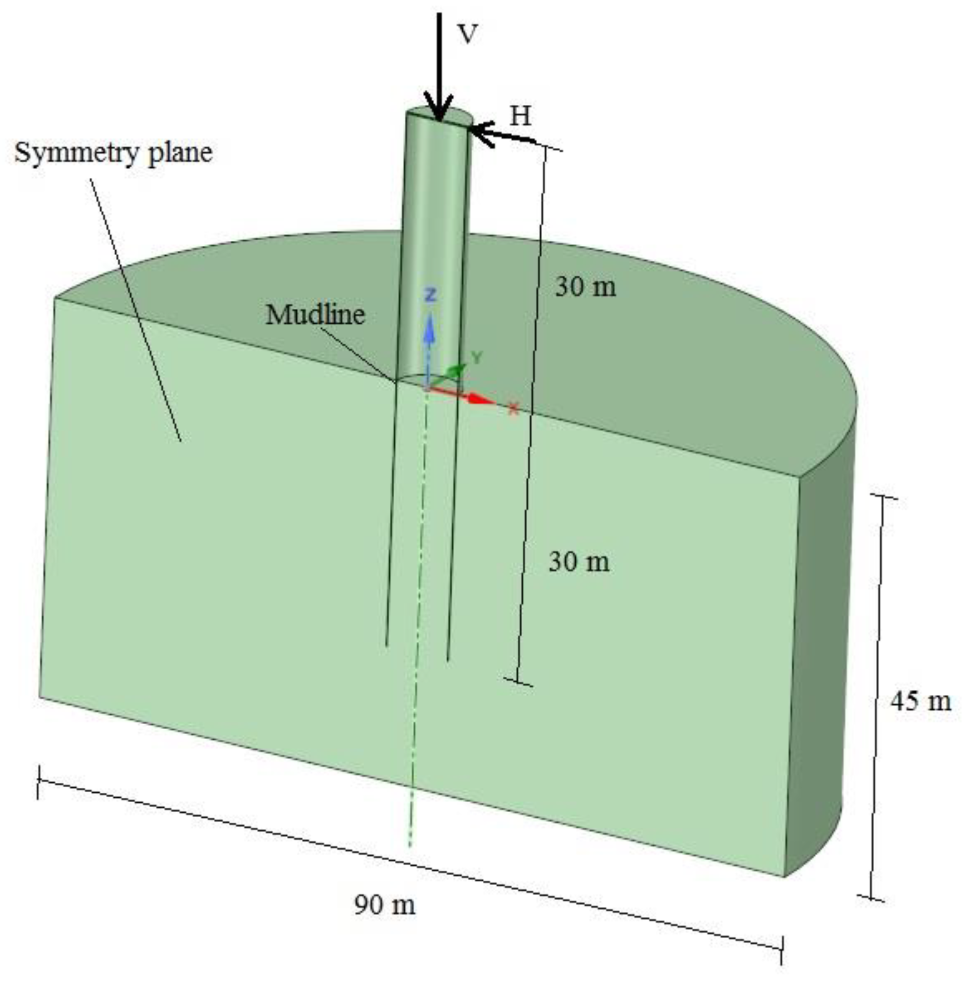
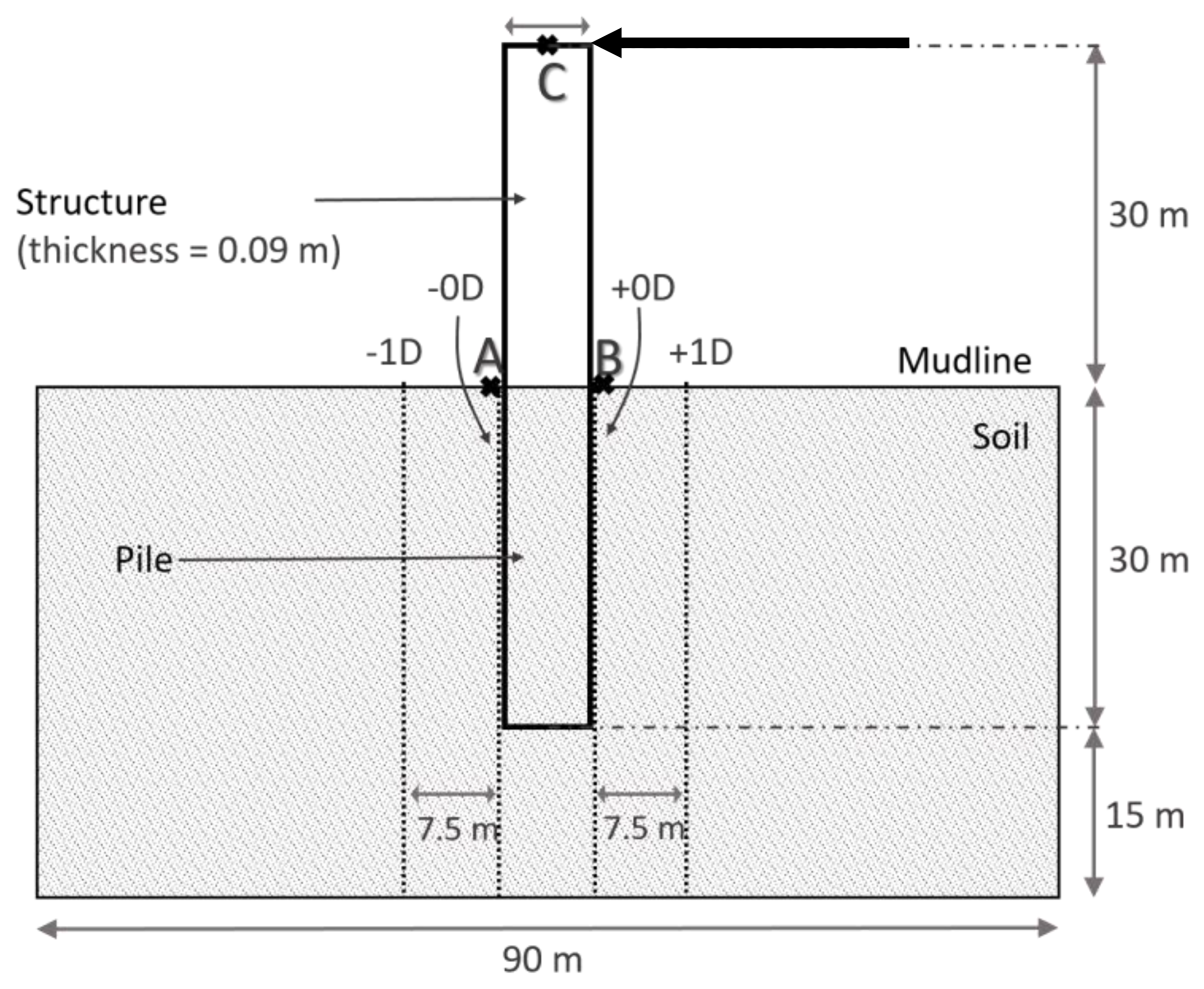
The full 3D hollow model consists of a hollow cylinder perfectly plugged, considering 30 m of elevation over the mudline and 30 m embedded in the soil, similar to the one analysed in [6]. The dimensions of this problem can be seen in Figure 1.
The static vertical load (to represent the weight of the turbine and remaining structure over 30 m) and the horizontal load (static or dynamic) are applied on top of the structure (i.e., 30 m above the mudline, which is assumed as the elevation where the resultant of the dynamic loads is applied). The application of loads at this point of the structure, instead of at the mudline, allows stresses to fully develop throughout the structure until the mudline, where the foundation starts. This aspect is very important to the development of equivalent models, for which equivalent stress levels will be targeted in the soil; the application of equivalent loads at the mudline level, instead of on top of the structure, might yield to different distributions for the lateral stresses throughout the pile in the different models. The possible oscillations in the radial orientation of this horizontal load (like the case reported in [31]) are neglected in this case, following the approach adopted by most existing FE simulations [6,7,15,32,33], and therefore, the problem is symmetric, and the symmetry plane is aligned with the applied horizontal load, as schematized in Figure 1. It is worth pointing out here that this 3D hollow model has been extensively validated against experiments, which demonstrates its goodness and validity [34,35,36]. Thus, in this paper, this model is considered as the best possible and most accurate option, and the developed simplified models are compared with it to assess their accuracy.
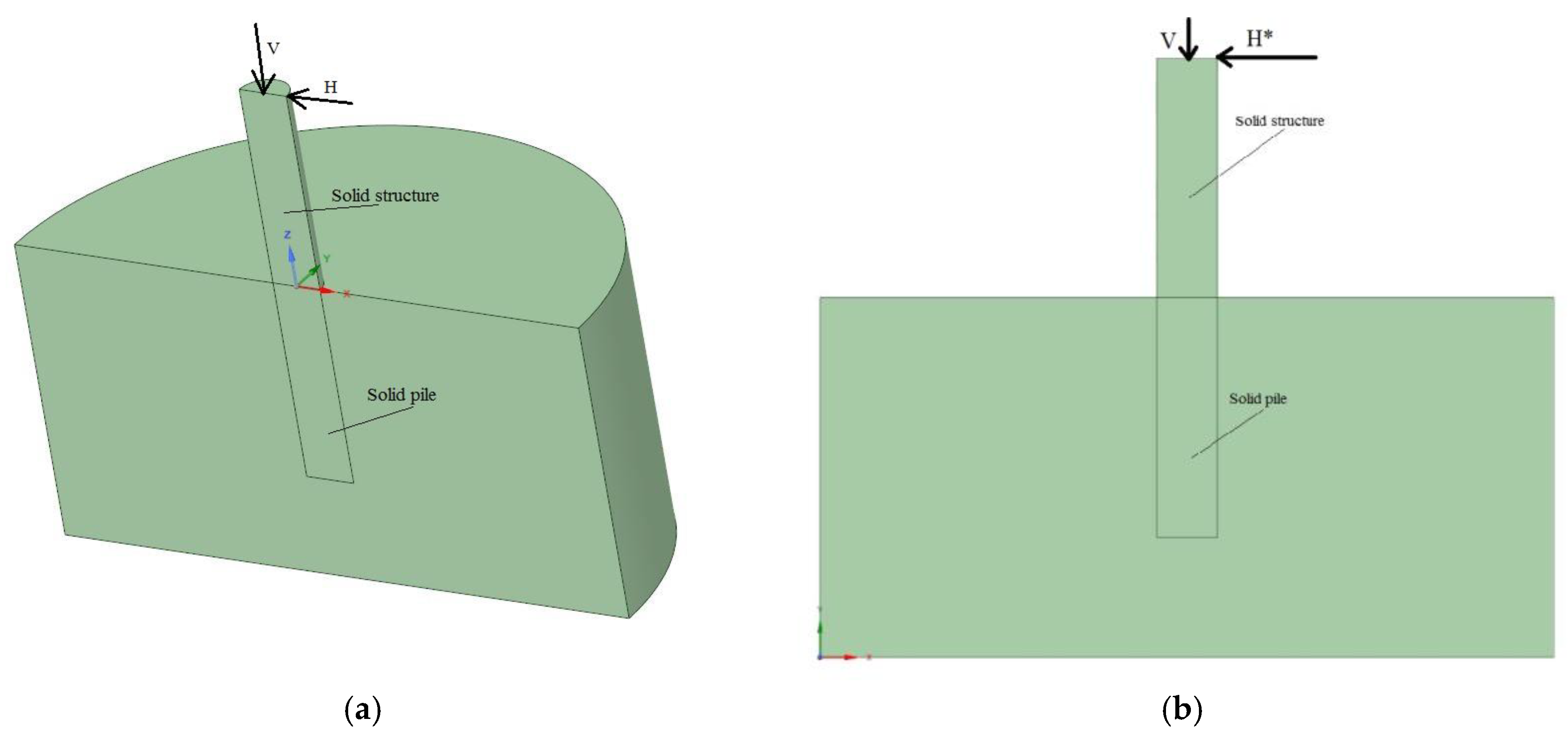
As previously mentioned, two simplified models, trying to replicate the previous one, were developed. The first one consists of a 3D solid structure (above the mudline) and a homogeneous solid pile (at the foundation level), with different properties to replicate the hollow steel part for the structure (above the mudline) and the embedded hollow pile at the foundation (below the mudline and assuming perfect plugging). The soil properties remain the same as in the original 3D hollow model.
The second simplified model is 2D, plane strain and solid, representing the symmetry plane of the 3D solid model only, where the higher stress and strain levels in the soil are expected to occur, i.e., those driving higher degradations in the long-term response of the infrastructure. The 2D model also consists of a solid structure over the mudline and a homogeneous solid pile below, both with equivalent properties as in the 3D solid model. The soil properties are again the same as in the 3D hollow model. The geometry of both simplified models can be seen in Figure 2.
3.2. Material Properties
Two types of soils have been considered in this research, a homogeneous soil and a heterogeneous soil (with depth-dependent elastic properties) with degradation. In the first case, the soil is assumed as isotropic and modelled with the elasto-plastic Mohr–Coulomb model [30]. Although this is a very simplified approach, it is suitable only for comparison purposes between the full and the simplified models at this first stage, which aims at understanding the suitability of simplified approaches under static and dynamic loads. The heterogeneous model, considering the degradation of the soil, accounts for more realistic conditions and is explored later in the paper. In all cases, the soil density has been assumed as saturated, neglecting pore water pressures. This approach is valid for comparison of the three models, and represents onshore conditions, but would be valid for offshore installations too by only replacing this value by the submerged density. As the soil properties are the same in all three models, the conclusions obtained from the comparisons remain valid.
As said, the homogeneous soil properties are the same in all three models and are those listed in Table 1.
The structure and pile are modelled as isotropic, linear elastic in all cases. In the first model, both pile and structure are assumed as a hollow steel cylinder, 0.09 m thick. For the simplified 3D solid model, the equivalent densities have been determined for both parts (structure and foundation—above and below the mudline, respectively) replicating the same weight as in the full model. The same equivalent densities are adopted in the 2D simplified model, which, as stated, represents the symmetry plane of the 3D problem (as sketched in Figure 2b).
The equivalent elastic moduli of structure and pile in both simplified models have been determined in order the keep the same flexural rigidity (EI) as in the structure and perfectly plugged foundation of the hollow pile, respectively. For the hollow structure, the flexural moment of inertia, I, is calculated for the hollow cylindrical shape (with the outer and inner radius), and E is the elastic modulus of the steel (given in Table 1). For the equivalent solid structure, I is obtained for a solid cylinder of 7.5 m of diameter (only the outer dimension matters in this case), and the equivalent elastic modulus is obtained in a way that EI remains as in the original hollow structure. The same procedure applies for the foundation part, below the mudline, where the perfectly plugged soil also has a flexural contribution. Again, in the case of the 2D solid model, the value has been adopted as the same as for the 3D solid simplified model to represent the central section of the wide pile.
The equivalent properties of the structure and pile parts in the simplified models are given in Table 1.
3.3. Input Loads
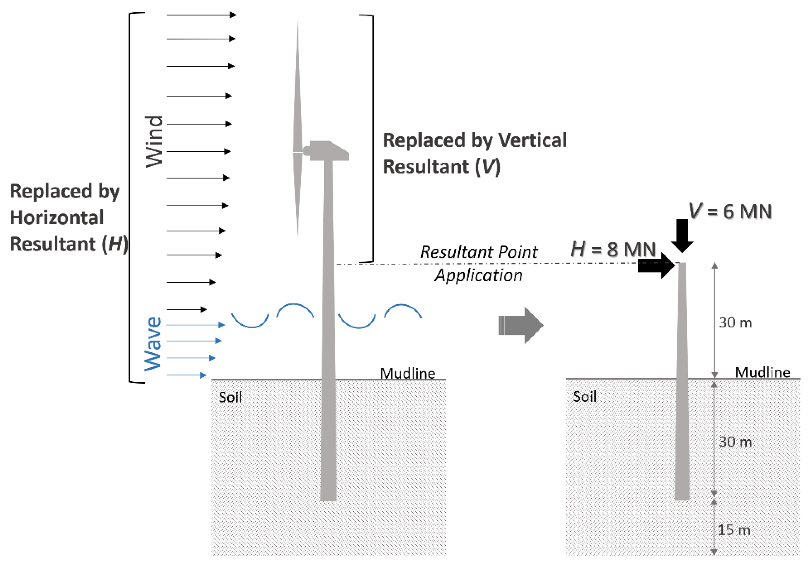
All models are initially subject to gravity load, to get initial stress conditions. After that, vertical and horizontal loads, as sketched in Figure 3, are applied on the resultant point, 30 m above the mudline. The vertical load corresponds to the weight of the turbine and the structure above that elevation, which are not included in the geometry of the model. The horizontal load, applied at the same point, represents the result of wind and, eventually, sea waves in the case of offshore locations.
The total vertical load is taken as 6 MN, while the peak value of the horizontal one is 8 MN. These values represent standard loads for 5 MW wind turbines. Due to the symmetry of the problem, both 3D models (hollow and solid) represent only half of the problem, and therefore the loads applied in the models are half of the total ones, i.e., V = 3 MN and H = 4 MN.
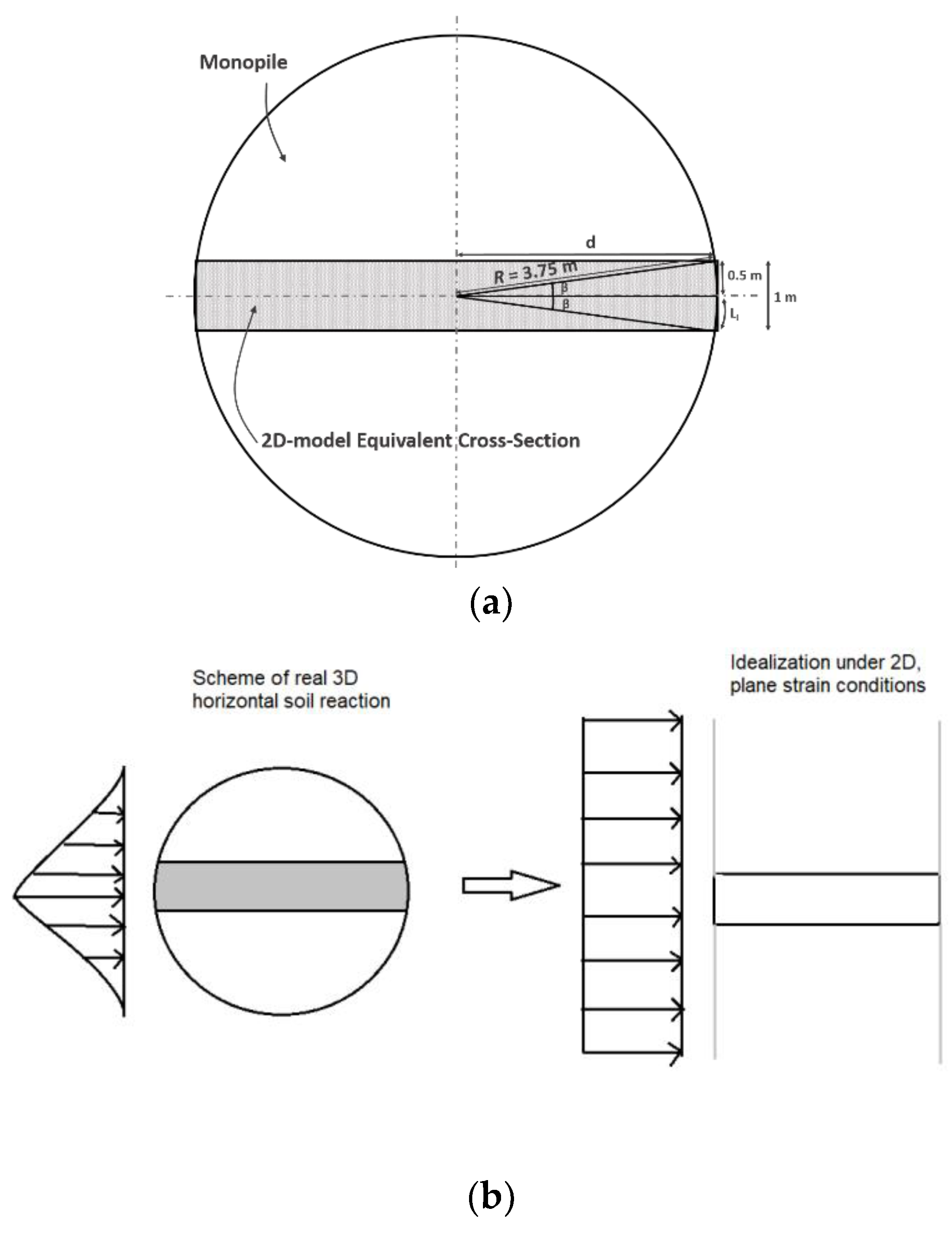
It is worth noting that this 2D model represents a great simplification of the problem, as it neglects the real 3D distribution of stresses in the soil–pile system (Figure 4b). The soil reaction under 2D conditions is overestimated, as illustrated in Figure 4b. Therefore, to properly represent the response of the pile, there are two options: either reducing the input load (to account only for the stresses in the central metre of the pile) or increasing the soil stiffness. The adopted approach is the first one, obtaining the equivalent load in the central metre of the pile, which is expected to represent fairly accurately the problem in the case of wide piles (as those usually employed in wind turbines). The stresses obtained with this model are given by metre of the problem in the dimension perpendicular to the geometry, and therefore the 2D equivalent vertical and horizontal loads represent the central metre of the problem (Figure 4). To determine the equivalent vertical load, a total 6 MN is assumed to be homogenously distributed over the circular cross-section of the structure, and then the total load in the central metre only is determined by proportionality of the areas of both cross-sections (see Figure 4a). For the equivalent horizontal load, it is assumed to be homogenously distributed throughout the length of the circumference (cross-section of the structure), and again, the resultant load only in the central metre of the problem is considered. Working along those paths, both values of equivalent loads for the 2D models are obtained (V* = 1.015 MN; H* = 0.681 MN).
Two types of simulations were conducted. The first one was static, while in the second one, the horizontal load was harmonic. In the latter, three load frequencies were considered (0.1, 1.0 and 2.0 Hz), aiming at exploring the effects of the frequency and its relationship with the natural frequencies of the models on the agreement between them. In all cases, both vertical (static in all cases) and horizontal loads were homogenously distributed on a thin, rigid plate on top of the structure to avoid localization of loads, particularly relevant in the case of the hollow model. In the case of harmonic loads, initially, two way loads were considered, following the next expression:
where h(t) represents the value of the horizontal load as a function of time, H (for the 3D models, or H* for the 2D model) is the amplitude of the horizontal load, as previously discussed, f is the frequency of the external load (in Hz) and t is the time.
3.4. Details of the Finite Element Model
Quadratic solid elements were adopted throughout the whole model to simulate both soil and pile-structure domains. In the case of the 3D models, the elements were tetrahedra for the soil and hexahedra for the pile. In the 2D model, both soil and structure–pile elements were triangles. The mesh was refined around the contact elements between soil and pile. Fixed support was assigned to the bottom boundary, while lateral horizontal constraints were applied to the exterior lateral sides of the soil. Gravity load was first applied to the model to obtain initial stress conditions, and then vertical and horizontal loads were applied on top of the structure, homogeneously distributed in a horizontal thin, rigid and weightless plate on top, to allow for a perfect stress distribution on the top cross-section.
The contact between soil and pile was modelled, in all cases, as frictional [30], with a friction coefficient of 0.4 [7]. In the case of the hollow model, this type of interface was also assumed in the inner part of the pile, while in the case of 3D and 2D solid models, it was only laterally considered.
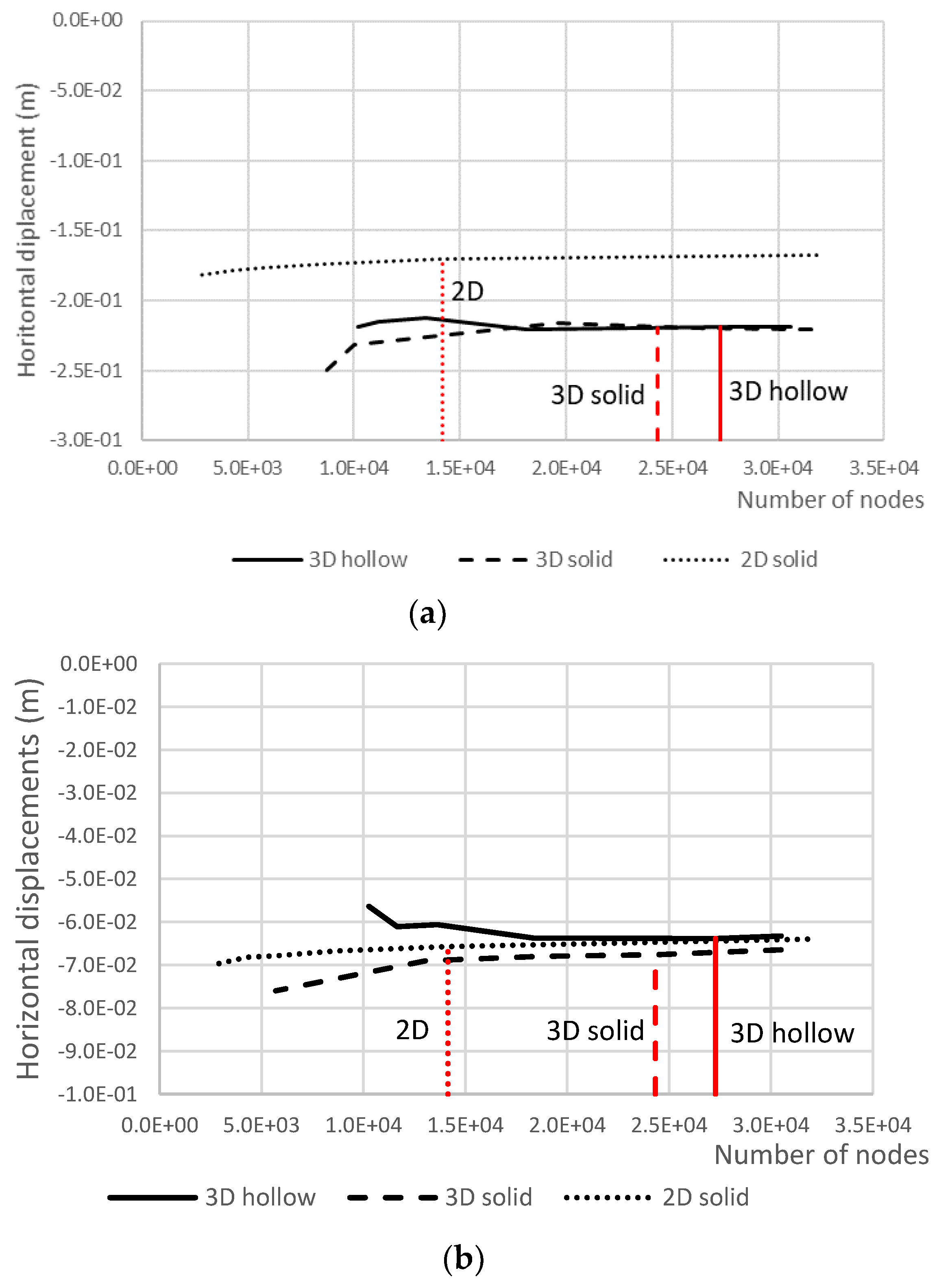
In order to select an accurate enough mesh for each model, a sensitivity analysis was undertaken, exploring the influence of different mesh densities. All three models were subjected to gravity, vertical and static horizontal loads. The horizontal displacements calculated on top of the structure and on point A of the soil (as indicated in Figure 5) for the models against the number of nodes are represented in Figure 6, from which the minimum mesh to guarantee an accurate enough solution could be justified. Based on this analysis, the models selected for the undertaken simulations were as follows: for the 3D hollow, 27,274 nodes; for the 3D solid, 24,396 nodes; for the 2D solid, 14,145 nodes. As can be seen in Figure 6, very little changes in the results were obtained for denser meshes in all cases. It is also worth noting that for the selected mesh densities, the solutions in terms of deformations and stresses were smooth, with no bubbles or sharp changes in the contours of solutions, as will be presented later. These meshes also allowed the convergence of the models under static and dynamic simulations.
4. Results and Discussion
4.1. Static Analysis
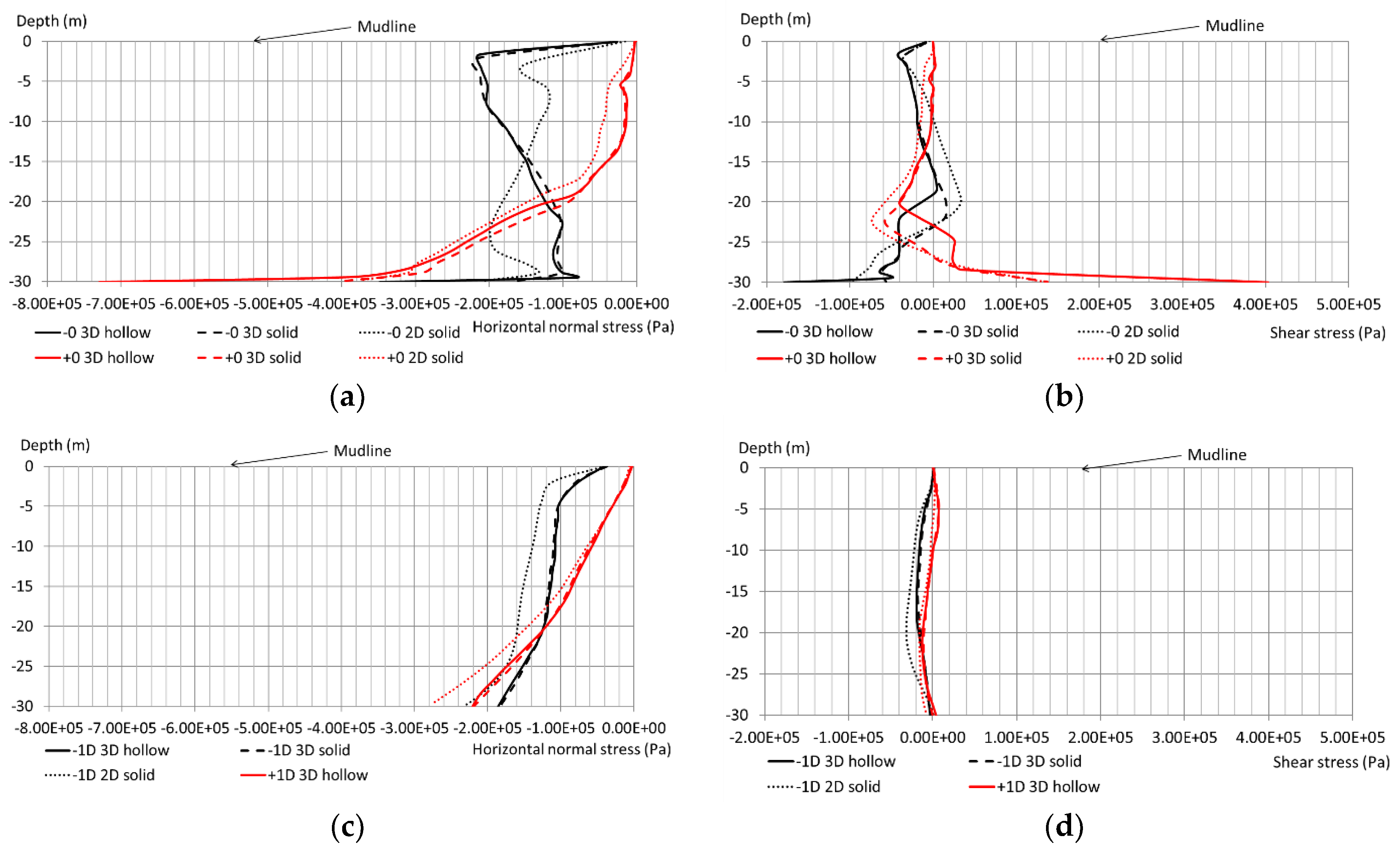
The comparison between solutions from all the above models under static loads, in terms of displacements (horizontal and vertical) and stresses (horizontal normal and shear), is presented next. In the 3D models, these solutions were obtained in the symmetry plane to allow for comparison with the 2D simulation. All these results are presented in vertical profiles. In what follows, −0 and +0 denote the profiles immediately on the left and the right-hand side of the pile (in the interface between soil and pile), respectively, while −1D and +1D refer to vertical profiles at 1 pile diameter (7.5 m) on the left and on the right of the pile, respectively (see Figure 5, where the direction of the horizontal load is also depicted).
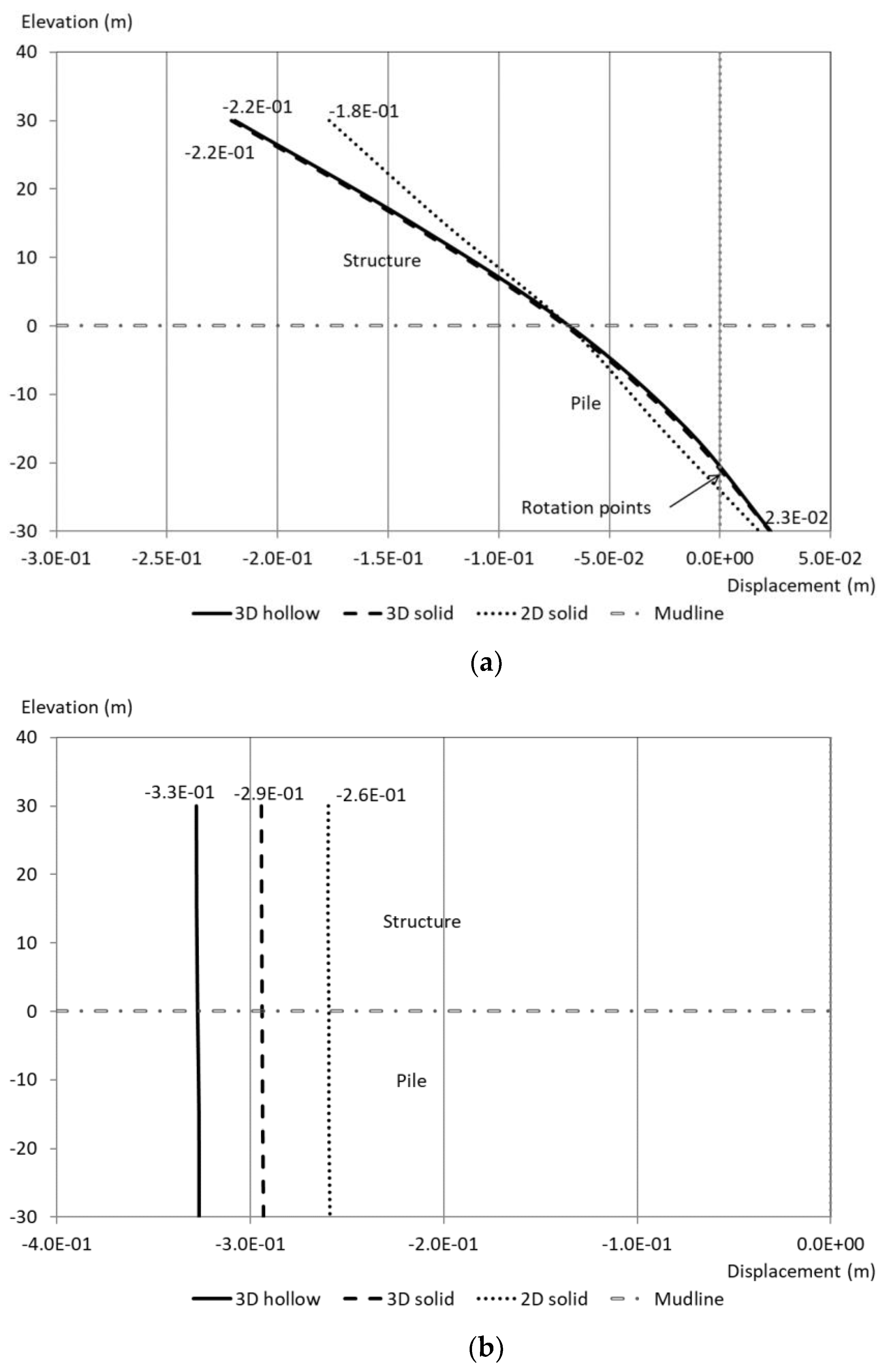
In Figure 7, the horizontal and vertical displacements in the central axis of structure and pile against depth, obtained with all three models, are represented and compared. For the horizontal displacements (Figure 7a) it can be concluded that the results obtained with 3D hollow and 3D solid models were almost identical at both structure and pile levels, while the 2D model slightly underestimated the displacements in the structure (with 0.18 m on top, while both 3D models yielded 0.22 m), but gave reasonably good agreement at the pile level, though displaying a more rigid behaviour (with less curvature). Regarding the vertical displacements in the structure-pile (Figure 7b), all three models predicted an almost constant settlement across the whole length of pile and structure (as the horizontal load had very little impact on the settlement), the solutions provided by both simplified models being smaller than for the 3D hollow model (settlements of 0.29 m and 0.26 m in the 3D solid and 2D), underestimating by 12% and 21%, respectively, the result of the 3D hollow model (which was 0.33 m). It can be therefore concluded that the simplified models yielded similar and moderately accurate results in terms of displacements in the structure-pile.
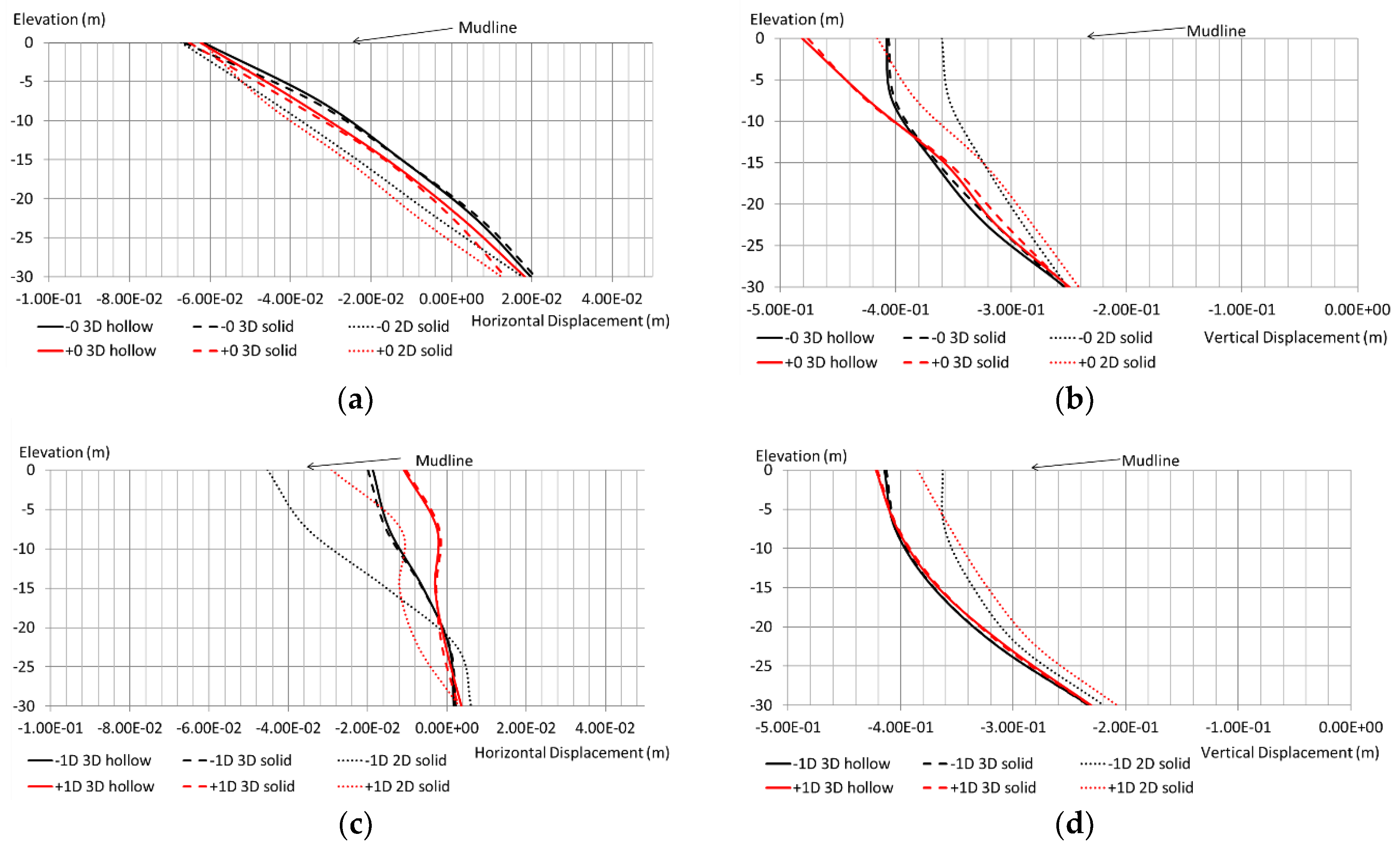
The horizontal and vertical displacements predicted by all models in the soil profiles (below the mudline) in −0, +0, −1D and +1D are represented in Figure 8. From these results, it can be concluded that the 3D solid model results were in almost perfect agreement with the 3D hollow, while the 2D simplified model gave moderately close results for horizontal and vertical displacements in the proximity of the pile (−0 and +0 profiles), while it slightly overestimated the horizontal displacements at −1D and +1D. It is remarkable that in all cases the 3D solid model provided highly accurate results.
The comparison between all static models in terms of horizontal normal and shear stresses is presented in Figure 9. The 3D solid model yielded very accurate results along with the pile for both normal and shear stresses, while the 2D solid model provided reasonably accurate solutions for shear stresses in all cases, as well as for normal horizontal stresses at +0 and +1D profiles, but it displayed worse agreements for the horizontal normal stress at −0 and −1D profiles, although these values were in the same range as for both 3D models. This is a logical result of the disparity previously discussed for the horizontal displacements at the same profiles obtained with the 2D model.
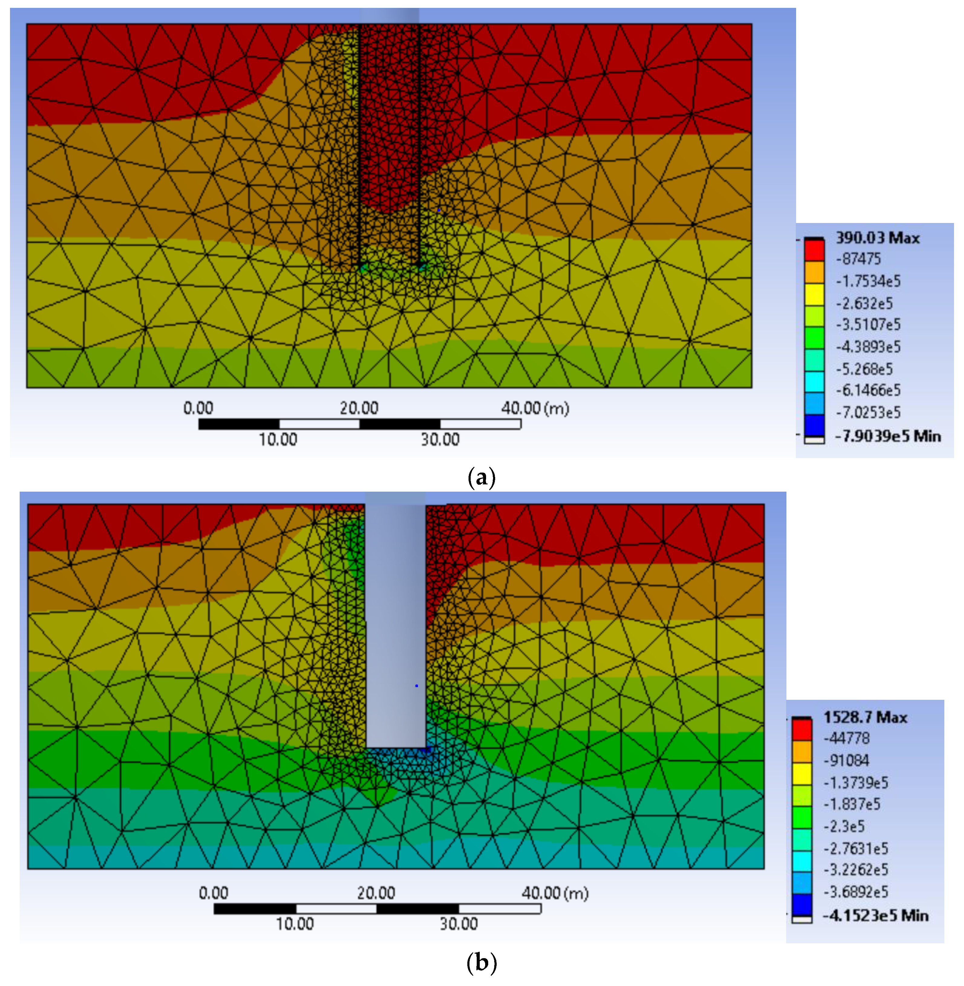
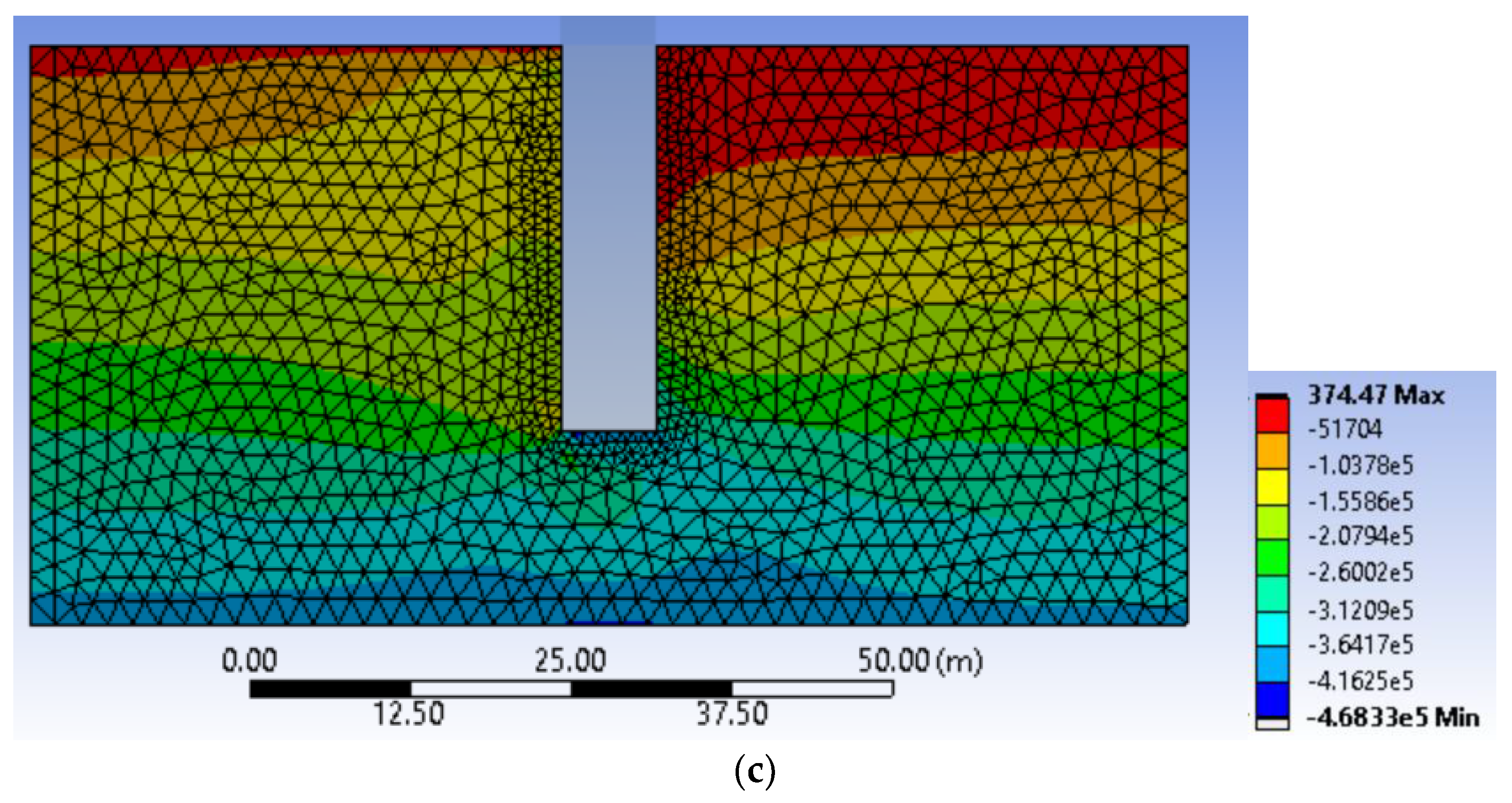
Some different local effects obtained with the 3D hollow model at the tip of the pile can be more clearly noted in Figure 10, where the horizontal normal stresses (i.e., in the direction perpendicular to the soil–pile vertical interface) are represented for the three models. It is worth noting that these figures represent the results only in the soil domain, which in the case of the 3D hollow model (Figure 10a) includes the inner part of the pile, while in the other two cases this is not included. In the figure, it can be seen that, despite the localised differences at the bottom of the pile, the three contours of solutions have similar appearance and values. We can therefore conclude that both simplified models were good enough to fairly represent the response of this soil–pile system under the static horizontal load applied in the symmetry plane of the model.
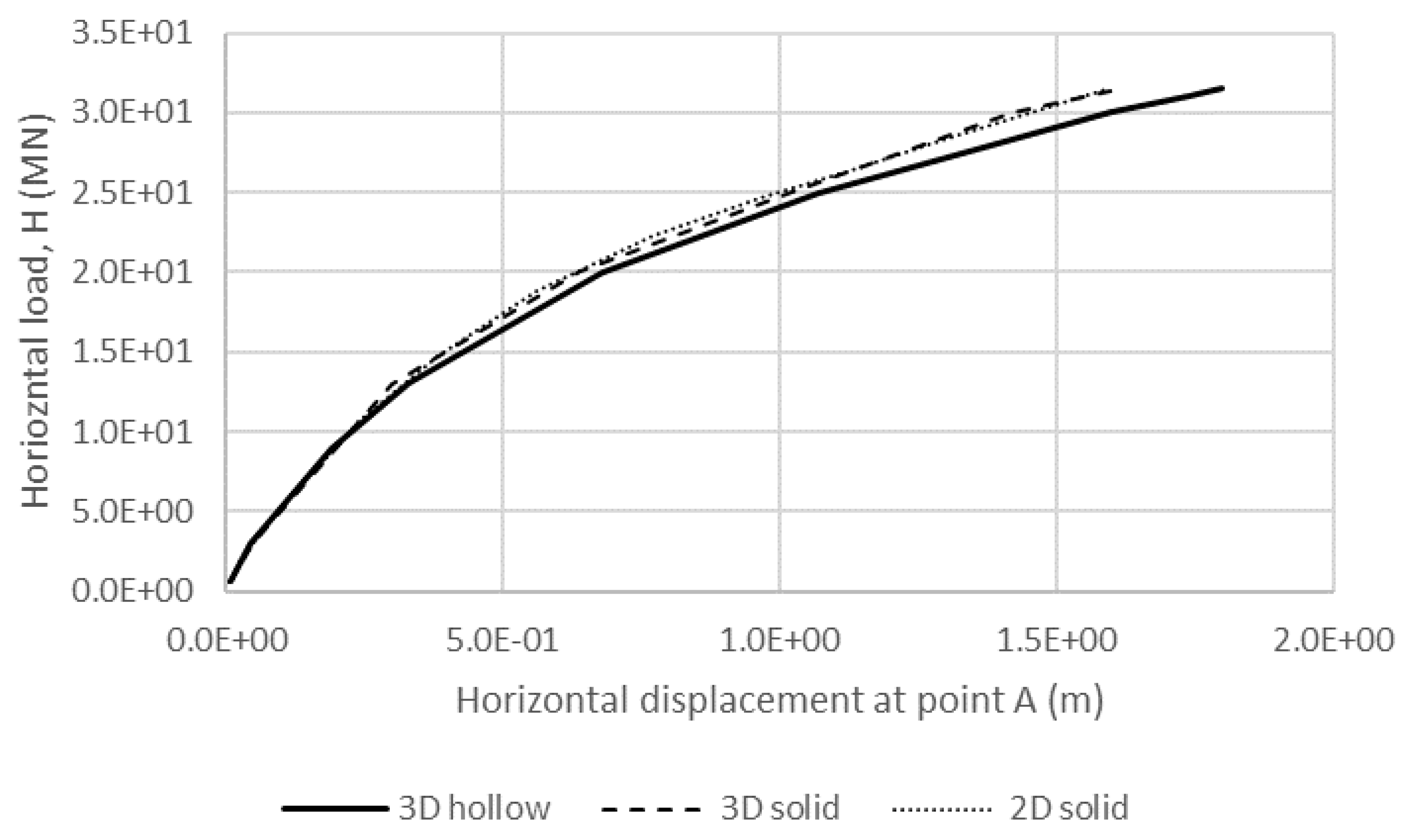
To explore the accuracy of the simplified approaches under a wider range of horizontal load values, the horizontal load–displacement curves (at point A of the soil—see Figure 5) were obtained for all three models and are represented in Figure 11.
It is important to explain herein that in the case of the 2D simplified model the load presented in the graph was the one for the full structure (H), while the numerical calculations for this model were made for the corresponding 2D equivalent values (H*), as worked out in Figure 4. The results demonstrate that the values obtained with both simplified models were accurate for the whole range of simulated horizontal loads, underestimating by around 10% the displacement of the full 3D hollow model in the case of the highest load (3.15 MN), which might be considered close to the ultimate lateral capacity of the pile. However, in the serviceability range of loads, the agreement was almost perfect. Therefore, quite remarkably, it is worth highlighting here that the initial stiffnesses obtained with all simulations were almost identical. This demonstrates that although the mechanisms for the soil–pile structure in the 2D simplified model were different than for the hollow or 3D solid pile, the behaviour in the symmetry plane of the problem was fairly well simulated, even under extreme load conditions.
4.2. Dynamic Analyses
In this section, the results obtained with all three models under dynamic loadings are presented and compared. As previously said, the vertical loads were the same as in the static simulations in all three models, but the horizontal loading on top of the structure was purely harmonic in this case (two ways in the case of the homogeneous soil—i.e., with positive and negative values—and one way in the stiffness degradation model), with an amplitude equal to the one employed in the static analyses. Firstly, and to evaluate the dynamic characteristics of the three models, their responses under free vibrations were investigated and compared. After this analysis, forced vibrations (with three different frequencies of the harmonic loading) were investigated, compared and discussed, based on the results obtained under free vibrations.
4.2.1. Free Vibration
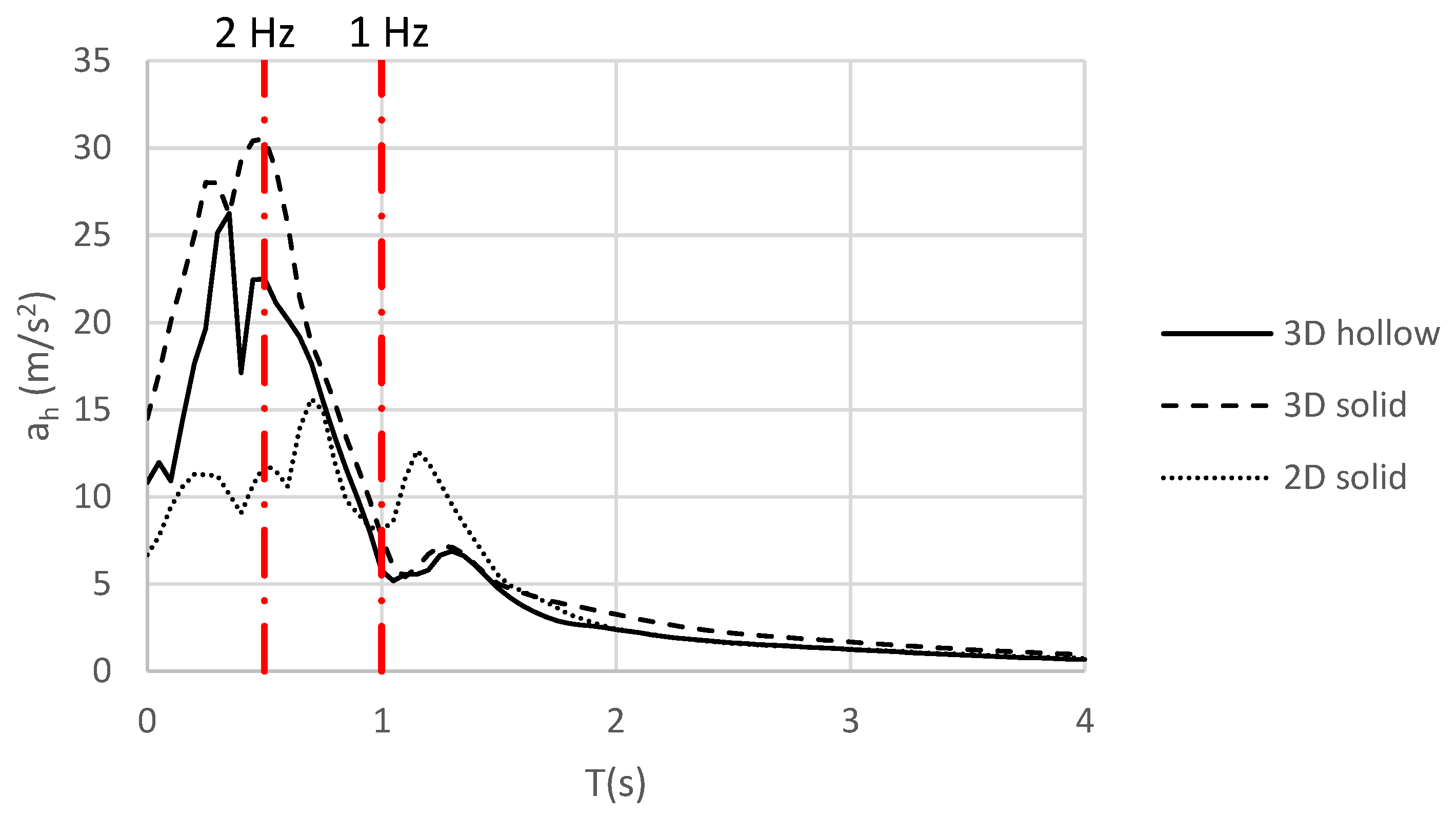
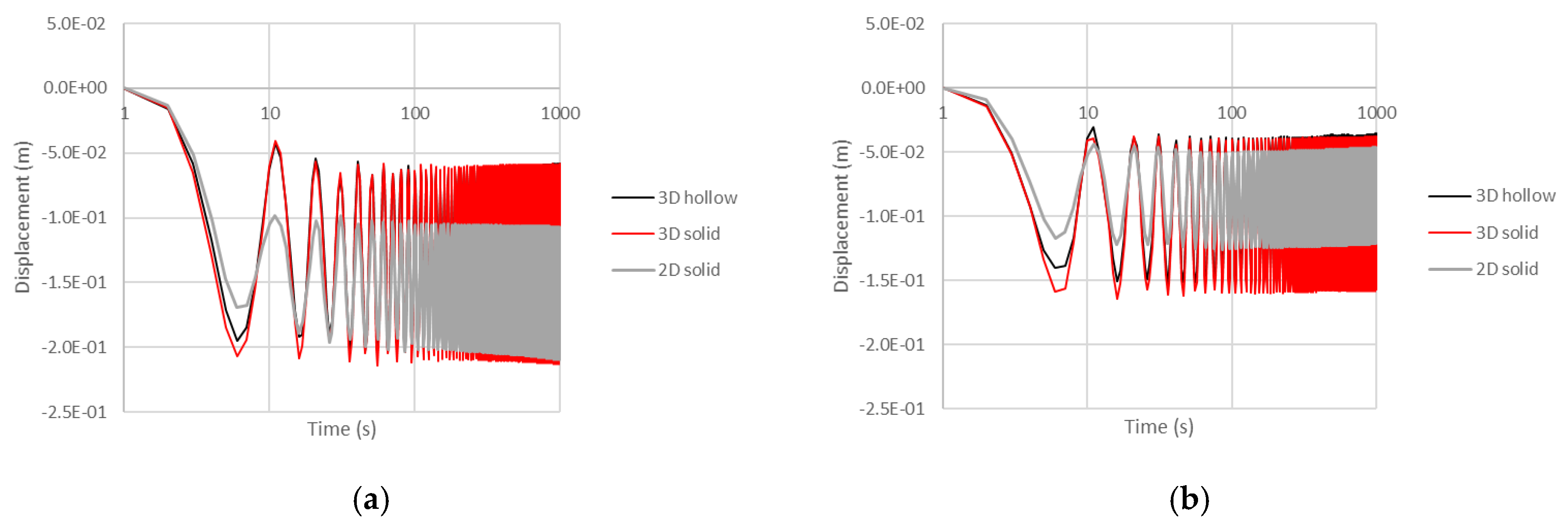
In this section, the same horizontal load previously employed for the static analysis was now slowly applied on top of the structure in each model and then suddenly released, so the systems were allowed to freely vibrate for 40 s. It is worth highlighting herein that the geometry, material properties and contact between the pile and soil were the same as for the static models. The time histories of horizontal accelerations on top of the structure during the free vibrations were recorded and employed to determine the elastic response spectra of accelerations (with 5% damping), which are represented in Figure 12.
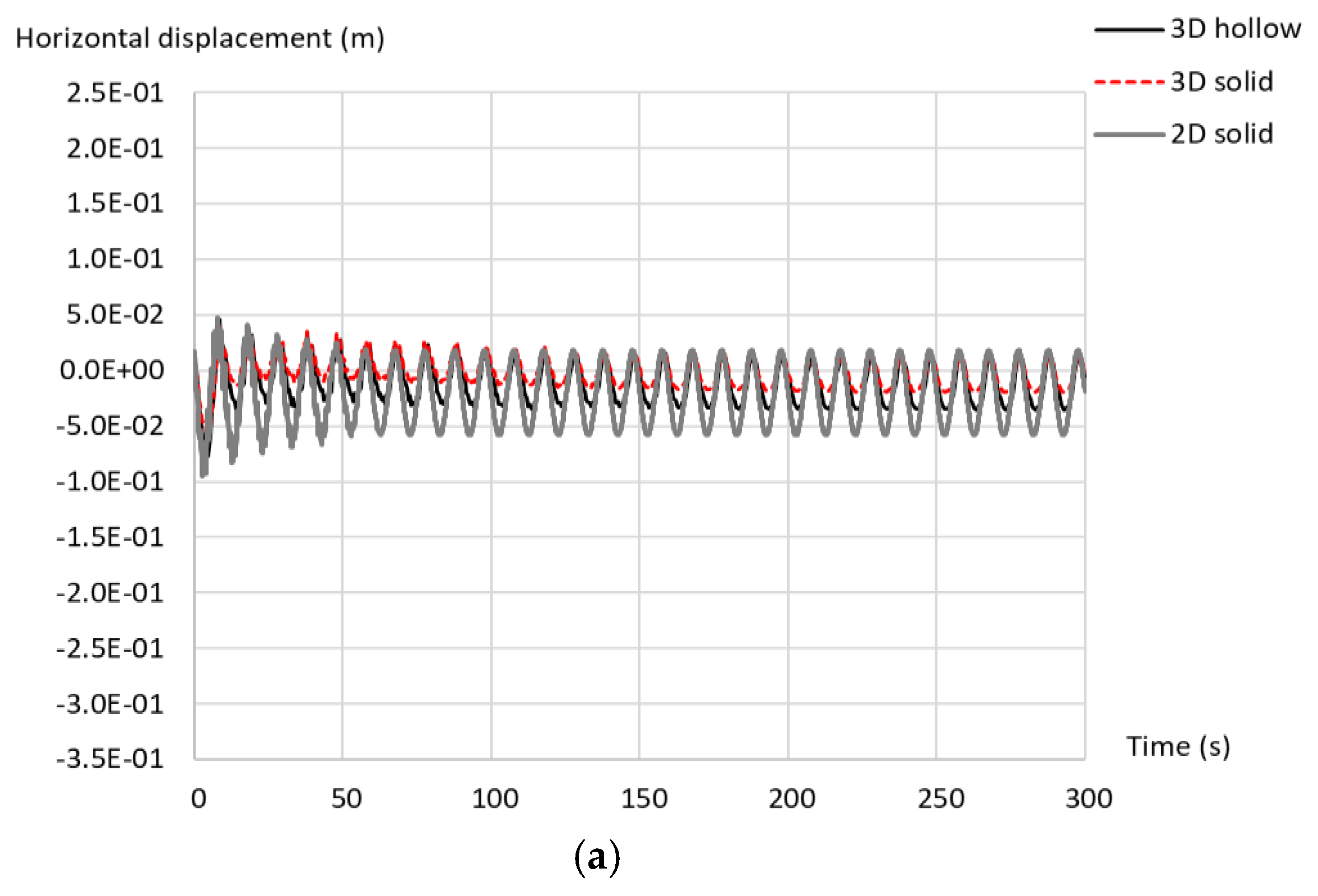
This comparison was undertaken on top of the structure (i.e., point C in Figure 5) as it was considered the most representative location to jointly evaluate and compare the vibration features for all three models. The figure highlights very similar dynamic responses on top of the structure in both 3D models (hollow and solid), showing only small differences between them for the lower periods, up to 1 s (i.e., frequencies higher than 1 Hz). Both models yielded to a peak value in response at around 0.5 s (slightly lower for the 3D hollow model) and a second and lower peak at T=1.35 s, values which can be interpreted as main response periods of these systems. The 2D simplified model, however, yielded to a significantly different dynamic performance, with the main peak value shifted to higher period with respect to the 3D models (at around 0.75 s) and a second peak found for T=1.15 s. It is worth noting that based on this comparison, for external cyclic loads with periods lower than 1 s (i.e., frequencies higher than 1 Hz), 3D models are expected to yield different responses compared to 2D models, at least for the peak values of the response, with the 3D solid being expected to reach higher amplitudes than the 3D hollow for this range of higher frequencies. On the contrary, it can be expected that all three models would result in similar peak responses for external loads with periods higher than or equal to 1.5 s (lower frequencies), for which all three spectra are almost coincident.
The different computational efforts for the three models are explored herein, based on the computational time taken by these free vibration models. The analyses were undertaken with a standard laptop, the same one in all cases. While the 3D hollow model took 371 min to conclude the analysis, the 3D solid model ended after 148 min (which represents a reduction of 60% of the time), and the 2D model finished in 21 min (which means a reduction of the 94%). These numbers are self-explanatory and highlight the relevance of a successful simplified simulation to save computational resources and to extend the time of simulation for dynamic events.
4.2.2. Forced Vibration in Homogeneous Soil
In this section, the three models were subjected to harmonic horizontal loading on top of the structure. Three different frequencies for the horizontal harmonic load (i.e., 0.1 Hz, 1.0 Hz and 2.0 Hz) were explored.
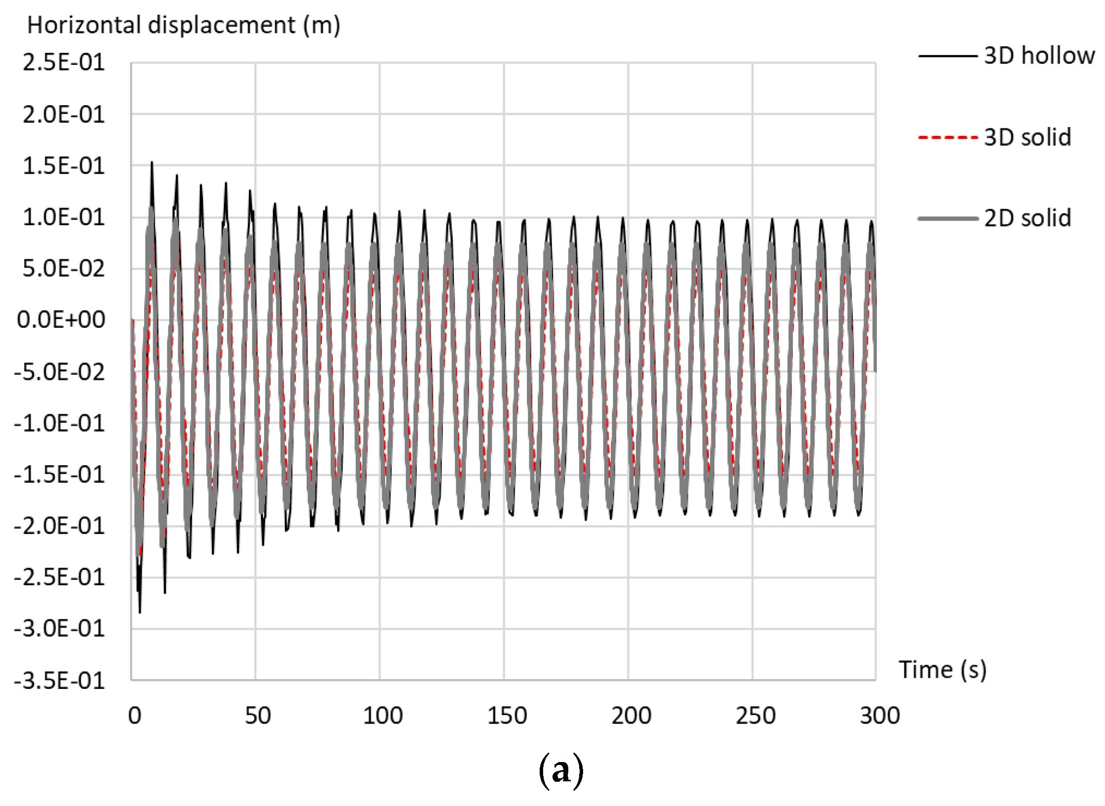
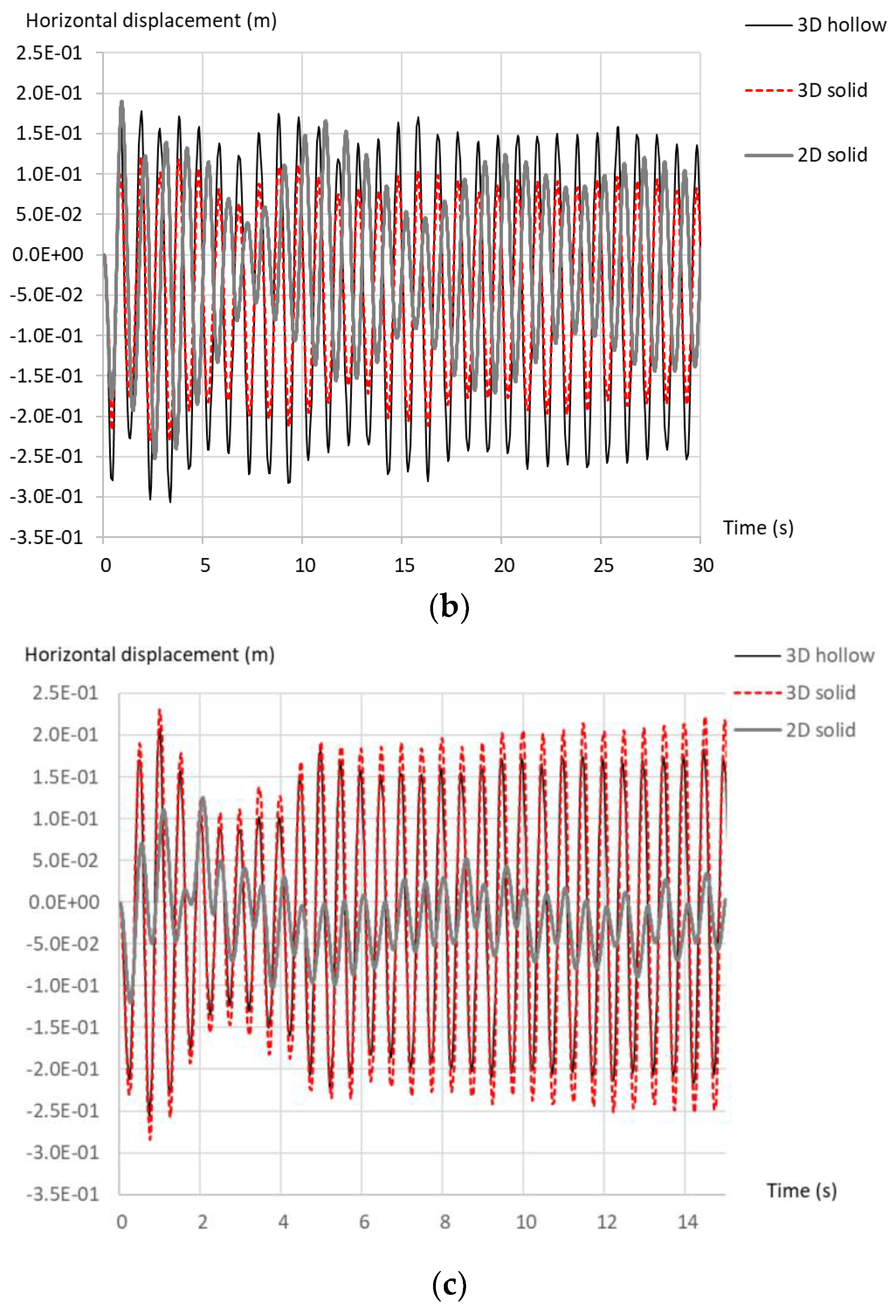
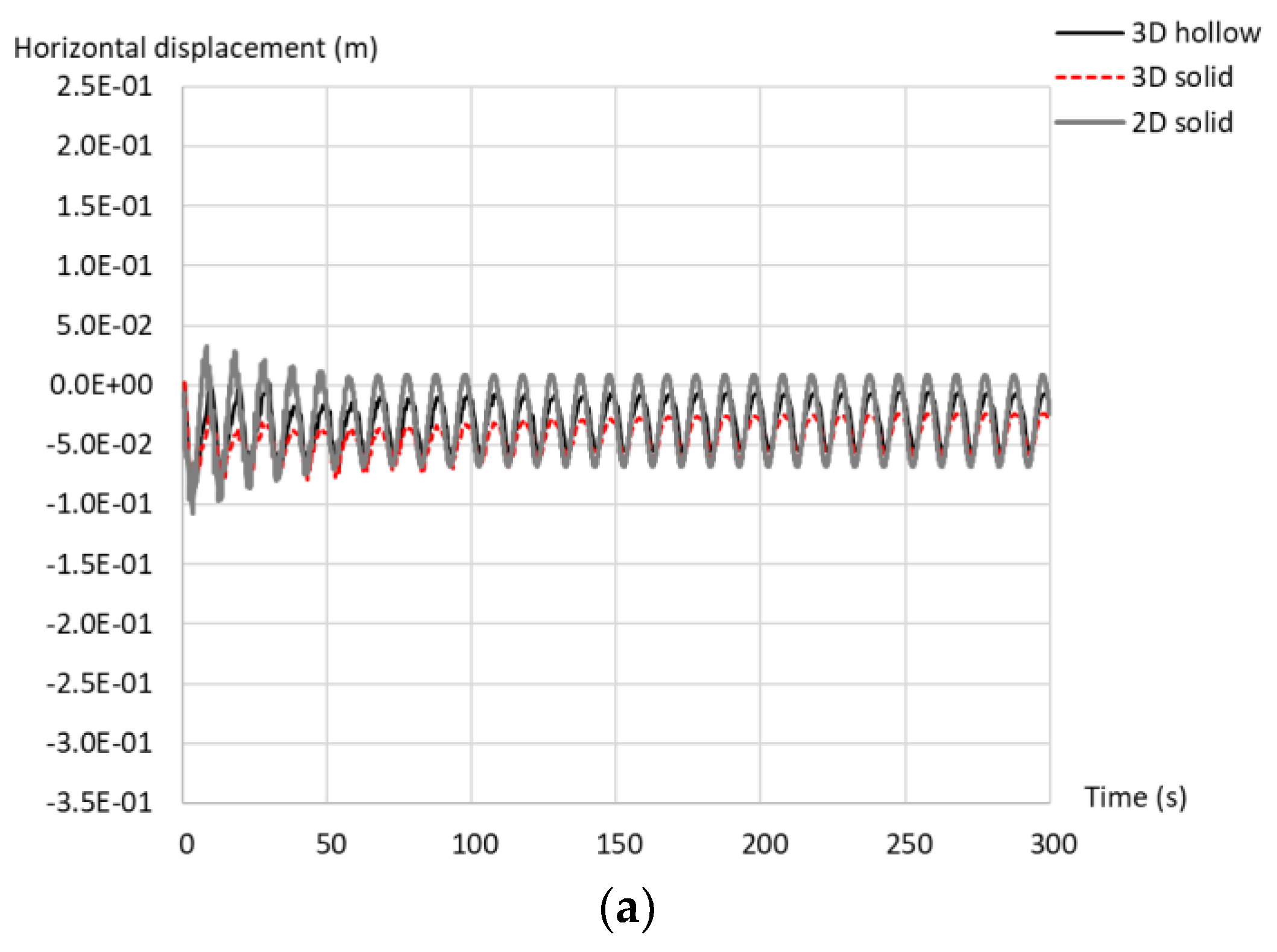
The history of horizontal displacements on top of the structure (point C in Figure 5) for the first 30 cycles and the three frequencies are presented in Figure 13. From this analysis, it can be concluded that the 3D solid model represented fairly well the dynamic behaviour of the 3D hollow system for all frequencies, particularly for 0.1 Hz (Figure 13a), slightly underestimating the amplitude of the response for 1 Hz and overestimating it for 2 Hz (by around 10% in both cases—see Figure 13b,c). In the case of the 2D model, it represented fairly well the dynamic behaviour for the lower frequencies (particularly for 0.1 Hz, and a bit worse for 1 Hz) and hugely underestimated it for the highest one. These results agree with the elastic response spectra presented in Figure 12, where it is clear that the spectrum for the 2D model at 2 Hz (period of 0.5 s) lay well below those of both 3D models. Moreover, although the peak values of the time history of displacements obtained with the 2D model for 1 Hz (Figure 13b) were in the same range of those obtained with both 3D models, it displayed a completely different pattern in the initial transient part, with a combination of the frequency of the external load and a slower response period of around 7 s. The amplitude of the response for this case, however, was in the same range as for the 3D models, which agreed with the elastic response spectra previously presented and discussed in Figure 12.
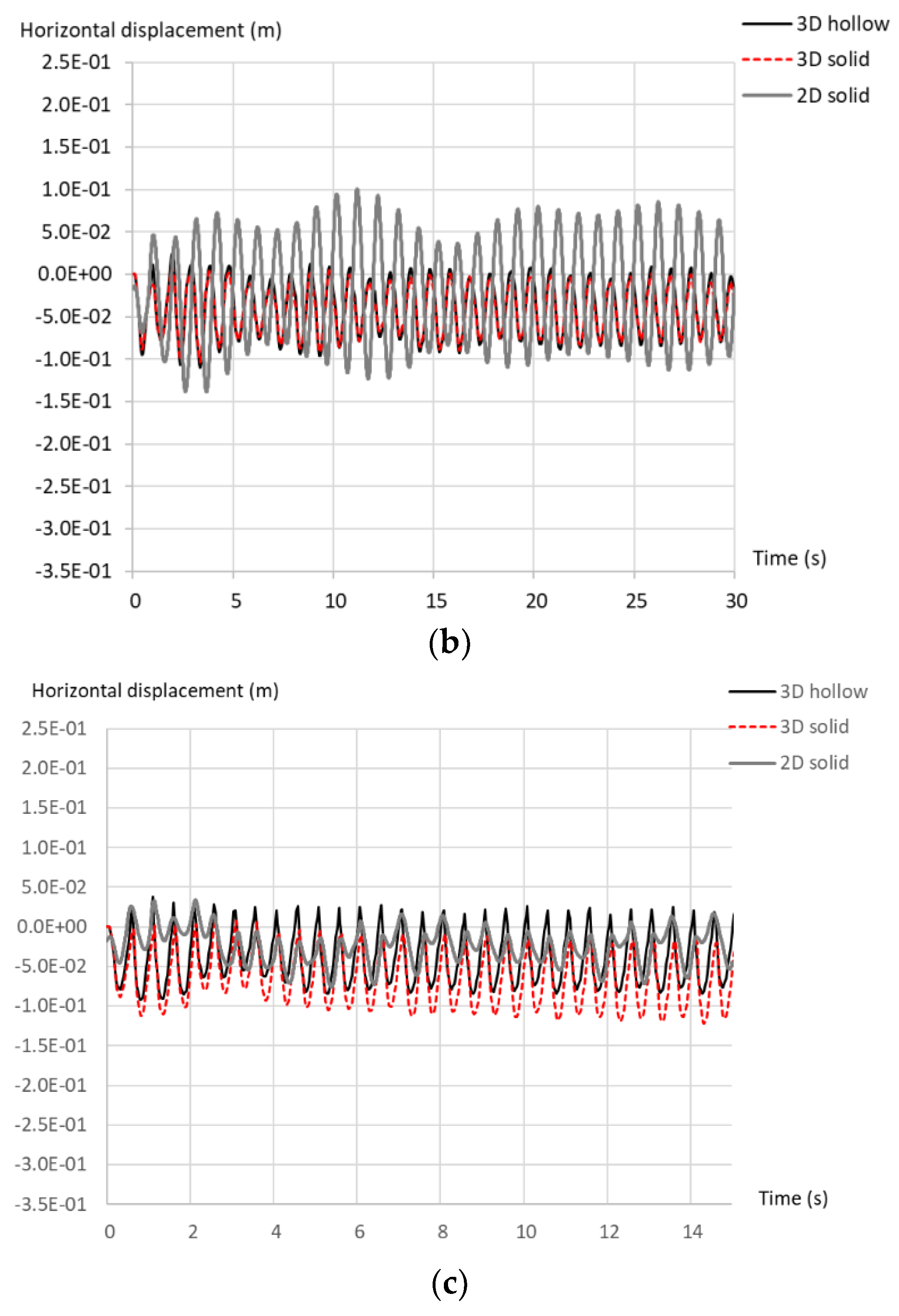
Similarly, Figure 14 and Figure 15 present the time history of horizontal displacements at points A and B in the soil (Figure 5), respectively. While the 3D solid model captured very well the dynamic response at those locations for all frequencies, the 2D model overpredicted the response for 1 Hz and underpredicted it for 2 Hz. The agreement for the lowest frequency in all cases was, however, remarkably good (as can be seen in Figure 14a and Figure 15a).
It can be therefore concluded that the simplified models provide reasonable solutions in terms of the amplitude of horizontal displacements, the results obtained with the 3D solid model being accurate for all frequencies, while the 2D model gives fairly accurate solutions for external loads with low frequencies. It is also interesting to note that, in general, the agreement is better at those locations in the soil rather than in the structure.
4.2.3. Forced Vibration in Depth-Dependent Stiffness Soil with Degradation
The approach presented by Achmus et al. [7] to consider heterogeneous soil profiles and degradation due to the accumulation of dynamic loads was adopted hereinafter. In this model, the elastic modulus of the soil, E, increased with depth according to the following expression:
where σat and σm, respectively, denote atmospheric pressure and mean principal stress, and and λ are model parameters. The soil degrades with the accumulation of cycles of loading, N. After the first cycle, the degradation rate of the secant stiffness, E1, is related to the value after N cycles, EN, as follows:
where is the plastic axial strain after N cycles, and denotes the plastic axial strain in the first cycle of load; b1 and b2 are model parameters, and X is the cyclic stress ratio, defined as
where is the major principal stress at failure under static conditions, and represents the major principal cyclic stress.
Two different soils were considered in these simulations: medium dense and dense sands. The elastic, nonlinear properties of these materials and the heterogeneity-degradation model parameters are listed in Table 2. The rest of properties required for modelling both sands (i.e., density, Poisson’s ratio, friction and dilatancy) were coincident for both soils and the same as in the homogeneous soil, for the sake of simplicity (Table 1).
In this case, and due to the nature of the model for the soil, one-way cyclic load was applied only (i.e., only positive values of the harmonic load), following the next expression:
A total of 100 cycles, with the same amplitudes (H for the 3D models, and H* for the 2D model) as in the previous simulations, and frequency f of 0.1 Hz, were applied in the three models.
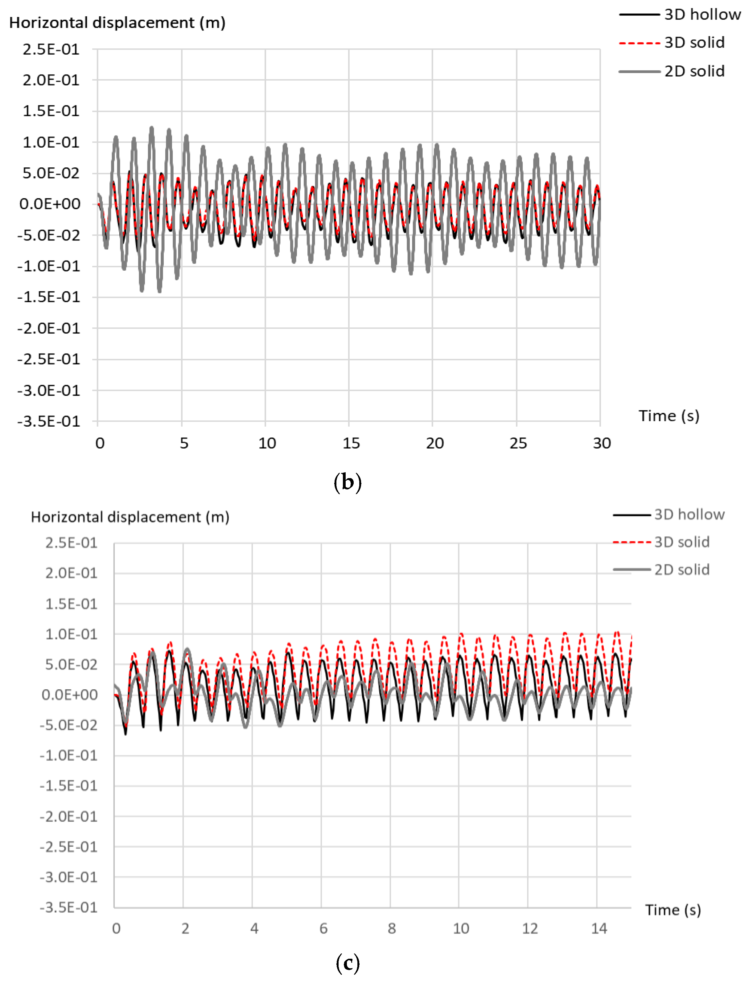
Figure 16 shows the displacements on top of the structure (point C in Figure 5) for all models and both materials. Figure 16a shows the results for medium dense sand, while those for dense sand can be seen in Figure 16b. These time history displacements demonstrated that both simplified models yielded very similar responses, with the 3D solid one closely replicating the response obtained with the 3D hollow, and the 2D model underestimating the amplitude of the oscillations, but capturing fairly precisely the maximum values for the medium dense material and the trends for both materials.
Finally, the comparison of the distribution of the horizontal normal and shear stresses in the first and 100th cycles are respectively presented in Figure 17 and Figure 18 for the three models and both types of soil in the −0 and +0 profiles. In these figures, apart from the comparison between the results obtained with all models, the effect of the degradation of the soil due to the repetition of loads can be quantified as the difference between the solutions at 1st and 100th cycles.
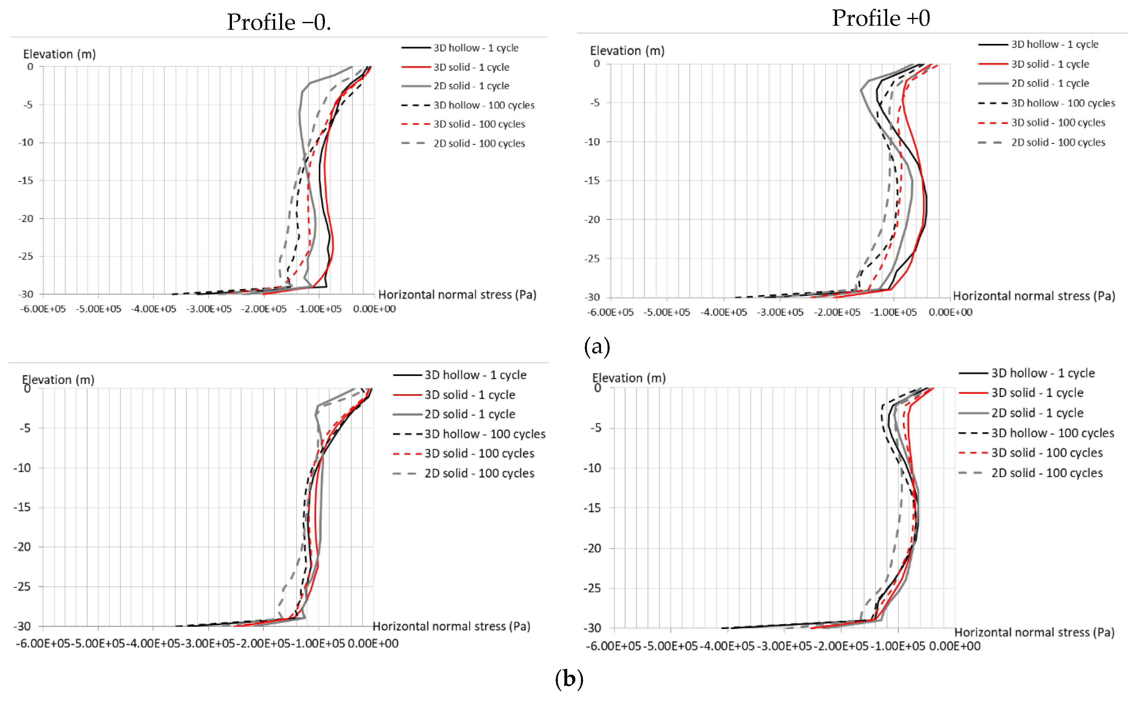
The comparison of horizontal normal stresses (Figure 17) highlights good agreement for all the models, particularly for the 3D solid compared to the full 3D hollow model, although the 2D model also yielded a reasonable accuracy, particularly at the +0 profile (similarly as in the case of the homogeneous soil) and for 100 cycles. This agreement was also better for the dense sand than for the medium dense material. From these figures, we can also conclude that the degradation effects, captured through the differences between the solutions for the 1st and 100th cycles, had a moderate effect, particularly for the dense sand, as expected. Interestingly, this effect was captured by the 2D solid model as well as by the 3D solid. Moreover, comparing these results with the distribution of the horizontal normal stress in the profiles nearby the pile, under static loads, for homogeneous soil (Figure 9a), we can conclude that the heterogeneity of soil had the effect of reducing the peaks in the solutions for all models, narrowing the differences between them and improving the agreement of the simplified models. It can also be concluded that the degradation of the soil, in terms of normal horizontal stresses, was only moderate.
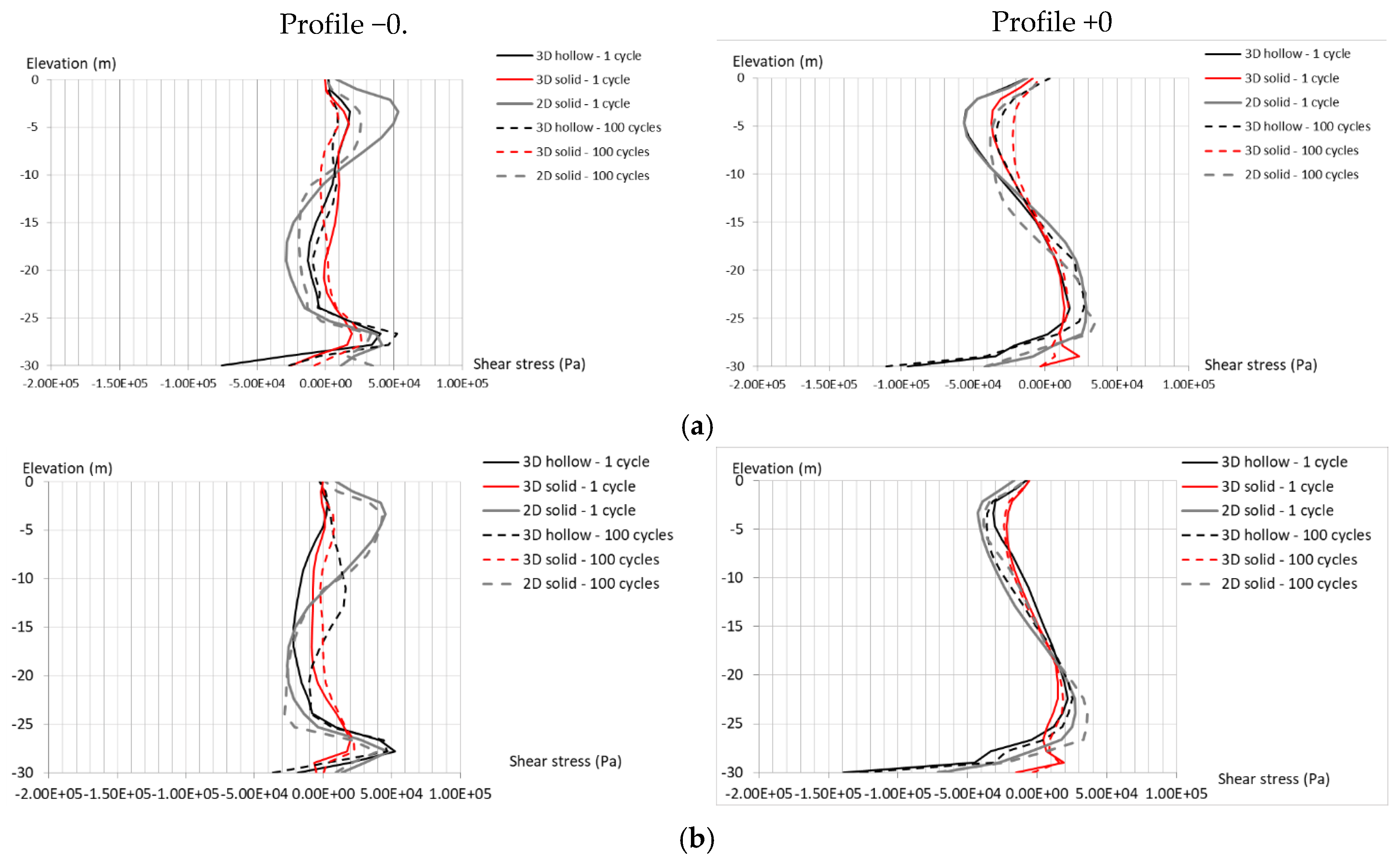
From the comparison in terms of vertical profiles −0 and +0 of shear stresses (Figure 18), it can be seen that the accuracy of the simplified models, when compared with the full 3D hollow, was reasonable, once again much better for the 3D solid than for the 2D, and yielding better overall results in the +0 profile. In all cases, the agreement was also better for the dense sand rather than for the medium dense (despite the local differences at the bottom of the pile, previously identified and discussed in the paper). As previously concluded, the differences between the 1st and 100th cycle were not substantial, and the agreement between the 2D model with the 3D hollow model improved with the number of cycles. As in the case of the normal stresses, in this case, also the effect of the degradation was seen as a reduction of the peak values as the number of cycles increased.
From the previously presented results, it can be concluded that the depth-dependent elastic properties, due to the relationship between stiffness and normal vertical stress, and the consideration of degradation effects, substantially improve the agreement between both simplified and 3D hollow models, particularly for the normal and shear stress distributions in depth. The degradation can be considered as an extra source of damping in the vibrating systems, thus making them less dynamic and more dissipative. This can also explain the better agreement in these cases.
5. Conclusions
This paper presents the derivation of two simplified numerical models, aiming at accurately replicating the response of a hollow wind turbine foundation to reduce the computational efforts for long term simulations. The first simplified model consists of a 3D solid structure and pile, while the second one is a 2D model which represents the central vertical section of the geometry. The equivalent properties of the solid equivalent geometries are justified using equivalent static flexure, while equivalent loads for the 2D model, which represents the symmetry plane of the problem only, are also determined. Static and dynamic simulations are presented and compared in the case of homogeneous, non-degraded soil, to explore their accuracy as well as the main dynamic features of all the models. The paper concludes with the consideration of heterogeneous material (with depth-dependent elastic properties) and soil degradation due to the accumulation of cycles of load. The main conclusions of this paper are as follows:
In the case analysed in this research, both simplified models provide accurate enough results under static conditions compared with the 3D hollow model; the agreement of the 3D solid model is almost perfect. The solutions, presented in terms of normal and shear stresses in the symmetry plane of the problem, are very similar in all simulations, apart from a local effect at the bottom of the pile in the hollow geometry caused by the much thinner connection between pile and soil in this area for this model compared with the simplified ones. Some differences are also observed in terms of horizontal displacements and normal stresses in the active side (left profile) of the soil for the 2D model. The comparison of the horizontal load–displacement curves for all models demonstrates that all of them yield identical initial stiffnesses, while the simplified models slightly underestimate the displacements for loads close to the ultimate lateral capacity of the pile.
The comparison of the free vibration of the three models (3D hollow, 3D solid and 2D solid), including the elasto-plastic soil behaviour and the frictional interfaces between soil and pile, highlights similar dynamic features of both 3D models for the whole range of periods, but a different response for the 2D model, with lower amplitude than for the 3D models for frequencies higher than 1 Hz, and very similar to those for slower external loads (i.e., lower frequencies), has been found.
The analyses of the forced response of the three models ratify the conclusions from the free vibrations, as the responses (in terms of displacements) obtained for both 3D models are very similar for all frequencies, while for those ranging between 1 and 2 Hz, the amplitude of the response obtained with the 2D model is much lower. The agreement obtained with all three models for the lowest frequency (0.1 Hz) is very good for the 2D model and excellent for the 3D solid.
The computational effort required for both simplified models is very much less than that for the 3D hollow approach, with reductions as large as of 60% and 94% for the 3D solid and 2D models, respectively.
When the soil is modelled as heterogeneous and its degradation (due to accumulation strains caused by repeated cycles of load) is considered, the agreement between simplified and full hollow models becomes much better, both in terms of displacements and stress distributions along with the pile. This agreement is excellent in the case of dense soil. The degradation of the soil, when 100 cycles are analysed, is proven to be very limited, particularly for the denser material.
This research demonstrates that simplified models can be employed as a suitable tool to balance accuracy and computational effort under the conditions presented in the paper and using the derived equivalent structure–pile properties and loads. This achievement will allow us to extend the time of analysis for wind turbine foundations, aiming at predicting their long-term response.
Author Contributions
Conceptualization, S.L.-Q. and M.S.; Literature review, P.J.M.M. and M.S.; Simulations: S.L.-Q., M.S. and J.A.-T.; Discussion and conclusions: all authors. All authors have read and agreed to the published version of the manuscript.
Funding
This research received no external funding.
Acknowledgments
The authors want the thank to the UK Engineering and Physical Sciences Research Council (EPSRC), Doctoral Training Partnership (DTP) grant EP/R513143/1 for University College London, for the financial support received by the second author, and to Comunidad Autonoma de Extremadura for the postdoctoral research international mobility grant covered by Decreto 200/2018-BOE, and to Fondo Europeo de Desarrollo Regional (FEDER) and Junta de Extremadura for funding granted to MATERIA research group (GR18122), received by the fourth author.
Conflicts of Interest
The authors declare no conflict of interest.
References
- Esteban, M.; Leary, D. Current developments and future prospects of offshore wind and ocean energy. Appl. Energy 2012, 90, 128–136. [Google Scholar] [CrossRef]
- Cuéllar, P. Pile Foundations for Offshore Wind Turbines: Numerical and Experimental Investigations on the Behaviour under Short-Term and Long-Term Cyclic Loading. Ph.D. Thesis, Technical University of Berlin, Berlin, Germany, 2011. [Google Scholar]
- Bhattacharya, S.; Nikitas, N.; Garnsey, J.; Alexander, N.; Cox, J.; Lombardi, D.; Wood, D.M.; Nash, D. Observed dynamic soil–structure interaction in scale testing of offshore wind turbine foundations. Soil Dyn. Earthq. Eng. 2013, 54, 47–60. [Google Scholar] [CrossRef]
- ISO. Petroleum and Natural Gas. Industries—Fixed Steel Offshore Structures; ISO: Geneva, Switzerland, 2007. [Google Scholar]
- DNV. Offshore Standard-Design of Offshore Wind Turbine Structures, DNV-OS-J101; Det Norske Veritas AS.: Oslo, Norway, 2014. [Google Scholar]
- Cuéllar, P.; Mira, P.; Pastor, M.; Fernández-Merodo, J.; Baeßler, M.; Rücker, W. A numerical model for the transient analysis of offshore foundations under cyclic loading. Comput. Geotech. 2014, 59, 75–86. [Google Scholar] [CrossRef]
- Achmus, M.; Kuo, Y.-S.; Abdel-Rahman, K. Behavior of monopile foundations under cyclic lateral load. Comput. Geotech. 2009, 36, 725–735. [Google Scholar] [CrossRef]
- Poulos, H.G.; Hull, T.S. The Role of Analytical Geomechanics. In Foundation Engineering: Current Principles and Practices; American Society of Civil Engineers: New York, NY, USA, 1989; Volume 2, pp. 1578–1606. Available online: https://cedb.asce.org/CEDBsearch/record.jsp?dockey=0063226 (accessed on 24 October 2020).
- Randolph, M.F. The response of flexible piles to lateral loading. Géotechnique 1981, 31, 247–259. [Google Scholar] [CrossRef]
- Niemunis, A.; Wichtmann, T.; Triantafyllidis, T. A high-cycle accumulation model for sand. Comput. Geotech. 2005, 32, 245–263. [Google Scholar] [CrossRef]
- Bransby, F. Difference between Load-Transfer Relationships for Laterally Loaded Pile Groups: Active p-y or Passive p -? J. Geotech. Eng. 1996, 122, 1015–1018. [Google Scholar] [CrossRef]
- Chen, C.-Y.; Martin, G. Soil–structure interaction for landslide stabilizing piles. Comput. Geotech. 2002, 29, 363–386. [Google Scholar] [CrossRef]
- Hazzar, L.; Karray, M.; Bouassida, M.; Hussien, M.N. Ultimate Lateral Resistance of Piles in Cohesive Soil. DFI J. J. Deep. Found. Inst. 2013, 7, 59–68. [Google Scholar] [CrossRef]
- Hazzar, L.; Hussien, M.N.; Karray, M. Two-dimensional modelling evaluation of laterally loaded piles based on three-dimensional analyses. Géoméch. Geoengin. 2019, 1–18. [Google Scholar] [CrossRef]
- Bourgeois, E.; Rakotonindriana, M.; Le Kouby, A.; Mestat, P.; Serratrice, J. Three-dimensional numerical modelling of the behaviour of a pile subjected to cyclic lateral loading. Comput. Geotech. 2010, 37, 999–1007. [Google Scholar] [CrossRef]
- López-Querol, S.; Cui, L.; Bhattacharya, S. Numerical Methods for SSI Analysis of Offshore Wind Turbine Foundations. In Wind Energy Engineering; Elsevier: Amsterdam, The Netherlands, 2017; pp. 275–297. [Google Scholar]
- Zdravkovic, L.; Taborda, D.M.G.; Potts, D.; Jardine, R.; Sideri, M.; Schroeder, F.; Byrne, B.; McAdam, R.; Burd, H.; Houlsby, G.; et al. Numerical modelling of large diameter piles under lateral loading for offshore wind applications. In Frontiers in Offshore Geotechnics III; Informa UK Limited: London, UK, 2015; pp. 759–764. [Google Scholar]
- McClelland, B.; Focht, J. Soil modulus for laterally loaded piles. J. Soil Mech. Found. Div. 1956, 82, 1–22. [Google Scholar]
- Reese, L.C.; Matlock, H. Non-dimensional Solutions for Laterally Loaded Piles with Soil Modulus Assumed Proportional to Depth. In Proceedings of the 8th Texas Conference on Soil Mechanics and Foundation Engineering, Austin, TX, USA, 14–15 September 1956. [Google Scholar]
- Reese, L.C.; Cox, W.R.; Koop, F.D. Analysis of Laterally Loaded Piles in Sand. In Proceedings of the Offshore Technology Conference, Society of Petroleum Engineers (SPE), Houston, TX, USA, 6–8 May 1974; Volume 2. [Google Scholar]
- Winkler, E. Die Lehre Von Elasticzitat Und Festigkeit; Scientific Research Publishing Inc.: Prague, Czech Republic, 1867; Available online: https://www.scirp.org/(S(vtj3fa45qm1ean45vvffcz55))/reference/ReferencesPapers.aspx?ReferenceID=2521358 (accessed on 24 October 2020).
- API. Planning, Designing, and Constructing Fixed Offshore Platforms, 22nd ed.; RP 2A-WSD.; American Petroleum Institute: Washington, DC, USA, 2014; Available online: https://infostore.saiglobal.com/en-us/Standards/API-2A-WSD-2014-98372_SAIG_API_API_206553/ (accessed on 24 October 2020).
- Achmus, M.; Albiker, J.; Peralta, P.; tom Wörden, F. Scale Effects in the Design of Large Diameter Monopoles; EWEA: Brussels, Belgium, 2011; pp. 326–328. [Google Scholar]
- Jardine, R.J. Geotechnics, energy and climate change: The 56th Rankine Lecture. Géotechnique 2020, 70, 3–59. [Google Scholar] [CrossRef] [Green Version]
- Randolph, M.F.; Dolwin, J.; Beck, R. Design of driven piles in sand. Géotechnique 1994, 44, 427–448. [Google Scholar] [CrossRef]
- Trochanis, A.; Bielak, J.; Christiano, P. Three-dimensional nonlinear study of piles. J. Geotech. Eng. ASCE. 1991, 117, 429–447. [Google Scholar] [CrossRef]
- Damgaard, M.; Bayat, M.; Andersen, L.V.; Ibsen, L.B. Assessment of the dynamic behaviour of saturated soil subjected to cyclic loading from offshore monopile wind turbine foundations. Comput. Geotech. 2014, 61, 116–126. [Google Scholar] [CrossRef]
- Ong, D. Benchmarking of FEM technique involving deep excavation, pile-soil interaction and embankment construction. In Proceedings of the 12th International Conference of International Association for Computer Methods and Advanced in Geomechanics (IACMAG), Goa, India, 1–6 October 2008. [Google Scholar]
- Sidali, R. Comparison between 2D and 3D analysis of mono-pile under lateral cyclic load. In Proceedings of the 5th Maghreb Conference in Geotechnical Engineering, Marrakech, Morocco, 26–27 October 2016. [Google Scholar]
- ANSYS. Available online: https://ec.europa.eu/eurostat/statistics-explained/index.php/Construction_production_(volume)_index_overview (accessed on 15 July 2020).
- Page, A.M.; Grimstad, G.; Eiksund, G.R.; Jostad, H.P. A macro-element model for multidirectional cyclic lateral loading of monopiles in clay. Comput. Geotech. 2019, 106, 314–326. [Google Scholar] [CrossRef]
- Page, A.M.; Skau, K.S.; Jostad, H.P.; Eiksund, G.R. A new foundations model for integrated analyses of monopile-based offshore wind turbines. In Proceedings of the 14th Deep Sea Offshore R&D Conference (EERA DeepWind’2017), Thondheim, Norway, 18–20 January 2017. [Google Scholar]
- Gelagoti, F.M.; Kourkoulis, R.S.; Georgiou, I.A.; Karamanos, S.A. Soil–Structure Interaction Effects in Offshore Wind Support Structures under Seismic Loading. J. Offshore Mech. Arct. Eng. 2019, 141, 061903-39. [Google Scholar] [CrossRef]
- Murphy, G.; Igoe, D.; Doherty, P.; Gavin, K. 3D FEM approach for laterally loaded monopile design. Comput. Geotech. 2018, 100, 76–83. [Google Scholar] [CrossRef] [Green Version]
- Shao, W.; Yang, N.; Shi, D.; Liu, Y. Degradation of lateral bearing capacity of piles in soft clay subjected to cyclic lateral loading. Mar. Georesources Geotechnol. 2019, 37, 999–1006. [Google Scholar] [CrossRef]
- Taborda, D.M.G.; Zdravković, L.; Potts, D.M.; Burd, H.J.; Byrne, B.; Gavin, K.G.; Houlsby, G.T.; Jardine, R.J.; Liu, T.; Martin, C.M.; et al. Finite-element modelling of laterally loaded piles in a dense marine sand at Dunkirk. Géotechnique 2020, 70, 1024–1029. [Google Scholar] [CrossRef] [Green Version]
Figure 1.
Geometry and dimensions of the 3D hollow model in the numerical simulations (V and H denote for vertical and horizontal loads applied on top of the structure).
Figure 1.
Geometry and dimensions of the 3D hollow model in the numerical simulations (V and H denote for vertical and horizontal loads applied on top of the structure).

Figure 2.
Geometry of the simplified equivalent models. (a) 3D solid model. (b) 2D solid model.

Figure 3.
Resultant vertical and horizontal loads on the resultant point application.

Figure 4.
Equivalent cross-section and resultant horizontal and vertical loads for the 2D-solid model. (a) Cross-section of 3D section and central metre of the pile (represented by the 2D model). (b) Idealization of the central metre of the pile under 2D, plane strain conditions and a sketch of horizontal soil reactions in both models.

Figure 5.
Vertical profiles and reference points employed in the comparison of the results between different models.
Figure 5.
Vertical profiles and reference points employed in the comparison of the results between different models.

Figure 6.
Sensitivity analysis of the mesh density for the different models. (a) Horizontal displacement on top of the structure; (b) horizontal displacement in point A (see Figure 5).
Figure 6.
Sensitivity analysis of the mesh density for the different models. (a) Horizontal displacement on top of the structure; (b) horizontal displacement in point A (see Figure 5).

Figure 7.
Displacements in the axis of structure and pile for the static problem obtained with the 3D hollow, 3D solid and 2D solid static models. (a) Horizontal displacements; (b) vertical displacements.
Figure 7.
Displacements in the axis of structure and pile for the static problem obtained with the 3D hollow, 3D solid and 2D solid static models. (a) Horizontal displacements; (b) vertical displacements.

Figure 8.
Displacements in the soil at the foundation level (below the mudline) obtained with 3D hollow and both simplified models, under static loading. (a) Horizontal displacements at −0 and +0; (b) vertical displacements at −0 and +0; (c) horizontal displacements at −1D and 1D; (d) vertical displacements at −1D and +1D.

Figure 9.
Stresses in the soil at the foundation level (below the mudline) obtained with 3D hollow and simplified models, under static loading. (a) Horizontal normal stress at −0 and +0; (b) shear stress at −0 and +0; (c) horizontal normal stress at −1D and 1D; (d) shear stress at −1D and +1D.
Figure 9.
Stresses in the soil at the foundation level (below the mudline) obtained with 3D hollow and simplified models, under static loading. (a) Horizontal normal stress at −0 and +0; (b) shear stress at −0 and +0; (c) horizontal normal stress at −1D and 1D; (d) shear stress at −1D and +1D.

Figure 10.
Horizontal normal stress (Pa) obtained in the plane of comparison with all three models under static conditions. (a) 3D hollow; (b) 3D solid, (c) 2D solid.
Figure 10.
Horizontal normal stress (Pa) obtained in the plane of comparison with all three models under static conditions. (a) 3D hollow; (b) 3D solid, (c) 2D solid.


Figure 11.
Horizontal load-displacement curves (at point A–see Figure 5) for the three models.
Figure 11.
Horizontal load-displacement curves (at point A–see Figure 5) for the three models.

Figure 12.
Comparison of elastic response spectra (5% damping) of accelerations for the models under free vibration on top of the structure.
Figure 12.
Comparison of elastic response spectra (5% damping) of accelerations for the models under free vibration on top of the structure.

Figure 13.
Comparison of horizontal displacements on top of the structure (point C in Figure 5) for different frequencies of external harmonic load: (a) 0.1 Hz, (b) 1.0 Hz, (c) 2.0 Hz.
Figure 13.
Comparison of horizontal displacements on top of the structure (point C in Figure 5) for different frequencies of external harmonic load: (a) 0.1 Hz, (b) 1.0 Hz, (c) 2.0 Hz.


Figure 14.
Comparison of horizontal displacements on top of the soil on the left side of the pile (point A in Figure 5) for the three frequencies: (a) 0.1 Hz, (b) 1.0 Hz, (c) 2.0 Hz.
Figure 14.
Comparison of horizontal displacements on top of the soil on the left side of the pile (point A in Figure 5) for the three frequencies: (a) 0.1 Hz, (b) 1.0 Hz, (c) 2.0 Hz.


Figure 15.
Comparison of horizontal displacements on top of the soil on the right side of the pile (point B in Figure 5) for the three frequencies: (a) 0.1 Hz, (b) 1.0 Hz, (c) 2.0 Hz.
Figure 15.
Comparison of horizontal displacements on top of the soil on the right side of the pile (point B in Figure 5) for the three frequencies: (a) 0.1 Hz, (b) 1.0 Hz, (c) 2.0 Hz.


Figure 16.
Comparison of histories of horizontal displacements in the heterogeneous, degradation model on top of the structure. (a) Medium dense sand; (b) dense sand.
Figure 16.
Comparison of histories of horizontal displacements in the heterogeneous, degradation model on top of the structure. (a) Medium dense sand; (b) dense sand.

Figure 17.
Profiles of horizontal normal stresses in the 1st and 100th cycles of load obtained with the three models at profiles −0 (left column) and +0 (right column). (a) Medium dense sand; (b) dense sand.
Figure 17.
Profiles of horizontal normal stresses in the 1st and 100th cycles of load obtained with the three models at profiles −0 (left column) and +0 (right column). (a) Medium dense sand; (b) dense sand.

Figure 18.
Profiles of shear stress in the 1st and 100th cycles of load obtained with the three models at profiles −0 (left column) and +0 (right column). (a) Medium dense sand; (b) dense sand.
Figure 18.
Profiles of shear stress in the 1st and 100th cycles of load obtained with the three models at profiles −0 (left column) and +0 (right column). (a) Medium dense sand; (b) dense sand.


Table 1.
Properties for the materials in the 3D hollow and both simplified models.
| Material | Young Modulus, E (MPa) | Poisson’s Ratio, ν | Density, ρ (Kg/m3) | Friction Angle, φ (o) | Dilatancy, δ (o) | Cohesion, c (kPa) |
|---|---|---|---|---|---|---|
| Soil (Mohr–Coulomb) | 40.0 | 0.25 | 2000.0 | 35 | 5 | 1 |
| Steel (elastic) | 2.1 × 10⁵ | 0.30 | 7850.0 | - | - | - |
| Structure (elastic—simplified models) | 1.94 × 10⁴ | 0.30 | 372.2 | - | - | - |
| Pile (elastic—simplified models) | 1.95 × 10⁴ | 0.30 | 2277.43 | - | - | - |
Table 2.
Model parameters for Achmus’ soil model.
| Type of Sand | Oedometric Stiffness Parameter, κ | Oedometer Stiffness Parameter, λ | Degradation Parameter, b1 | Degradation Parameter, b2 |
|---|---|---|---|---|
| Medium dense | 400 | 0.60 | 0.16 | 0.38 |
| Dense | 600 | 0.55 | 0.2 | 5.76 |
Publisher’s Note: MDPI stays neutral with regard to jurisdictional claims in published maps and institutional affiliations. |
© 2020 by the authors. Licensee MDPI, Basel, Switzerland. This article is an open access article distributed under the terms and conditions of the Creative Commons Attribution (CC BY) license (http://creativecommons.org/licenses/by/4.0/).
Share and Cite
MDPI and ACS Style
Lopez-Querol, S.; Spyridis, M.; Moreta, P.J.M.; Arias-Trujillo, J. Simplified Numerical Models to Simulate Hollow Monopile Wind Turbine Foundations. J. Mar. Sci. Eng. 2020, 8, 837. https://doi.org/10.3390/jmse8110837
AMA Style
Lopez-Querol S, Spyridis M, Moreta PJM, Arias-Trujillo J. Simplified Numerical Models to Simulate Hollow Monopile Wind Turbine Foundations. Journal of Marine Science and Engineering. 2020; 8(11):837. https://doi.org/10.3390/jmse8110837
Chicago/Turabian StyleLopez-Querol, Susana, Michail Spyridis, Pedro J. M. Moreta, and Juana Arias-Trujillo. 2020. "Simplified Numerical Models to Simulate Hollow Monopile Wind Turbine Foundations" Journal of Marine Science and Engineering 8, no. 11: 837. https://doi.org/10.3390/jmse8110837
Note that from the first issue of 2016, this journal uses article numbers instead of page numbers. See further details here.