Critical Water Depth and Installation Curves for Submarine Cable Deployment Process

Abstract

The purpose of the present paper is to propose installation curves for submarine cable deployment process for different water depths and tension deployment, emphasizing on the importance of modelling the “out of water” cable segment and the friction force between cable and overboard chute of the installation vessel. A custom-made analysis tool has been further expanded and used for the calculation of the cable hydraulic critical responses. Moreover, the concept of the critical water depth is proposed analytically for first time to define the cases in which the “out of water” cable segment can be ignored without denoting the accuracy of the minimum bending radius calculation. In addition, correction factors are proposed in relation to water depth and bottom tension values in order to eliminate the error of the safety factor calculation. Numerical formulation of the friction has been incorporated in the custom-made analysis tool as a further development. The analysis of various cable deployment cases proves that the inclusion of the “out of water” segment in the analysis is critical in shallow water areas. In contradiction, the modelling of the friction force is critical in deep water areas. However, both parameters are potential causes of important analysis errors.

1. Introduction

Submarine cable systems are a vital and expanding part of the worldwide power supply and telecommunication networks. The installation of a submarine cable system is a demanding and complex task [1]. Factors such as cable mechanical properties, route irregularities and characteristics, available equipment and capacities of the cable installer are taken into consideration during the planning phase by the cable route planning and installation analysis [2]. Some of the most critical and influential parameters for a cable S-lay installation are presented in Figure 1 and briefly discussed in [3]. A cable installation curve is defined by the following parameters: Exit angle (θ) is the angle defined between the horizontal axis X and the axis of the cable at the overboard chute of the Cable Lay Vessel (CLV). Top tension (T_tensioner) is the tension applied along the axis X to the cable using the onboard constant tension machine, just before the overboard chute. Friction (Fr) at the cable chute is the resistant force created due to the contact between the cable and the overboard chute of the CLV. Layback (LB) is the horizontal distance between the last point of cable touching on the overboard chute and the touch down point (TDP) on the seabed. Catenary length (CL) is the length along the deformed axis of the cable between the cable exit point from the CLV and the TDP on the seafloor. Bend radius is the actual cable radius of curvature which should be maintained within the allowable limits recommended by the cable manufacturer. Minimum bending radius (MBR) is the actual minimum bend radius along the combined catenary curve during the laying process. Bottom tension (H) is the residual internal force of the cable at the TDP, crucial parameter during a cable S-lay installation.

Cable handling and monitoring is important during the cable laying process as the cable can be damaged if the minimum bending radius, actual strain, or other limits are not respected during installation. The use of the state-of-the-art cable lay analysis tools allow the effective control of the vessel and the cable handling systems available onboard and provide the cable installer with the most thorough and accurate information possible on cable conditions during the laying process such as: accurate cable touch down location (for future reference, recoveries and repair), cable bottom tension (to minimize unwanted cable suspensions on uneven seafloors), and cable loads (to properly handle the low tensile strength of the new generation cables or avoid cable compression loads on the seabed).

Numerous theories and analysis approaches have been developed, based on different assumptions, for the static and dynamic response of a submarine cable during installation in an S-lay configuration. One of the first theories describing the cable laying problem developed by Zajac [4], using a steady-state theory in which the cable was modelled as a straight line excluded any effect of transient motions. Specifically addressing the issue of cable dynamics, Walton and Polachek [5] presented a two-dimensional solution for the transient analysis of towed marine cables using a finite element model utilizing finite difference methods. Few years later, an analytical theory for tension analysis of cables without considering the tangential drag forces presented by Yoshizawa and Yabuta [6]. A prediction model for the 2D cable transient behavior taking into consideration external hydrodynamic loads was developed and presented by Vaz and Patel [7] and recently by Abidin et al. [8,9]. Following their previous work, Vaz et al. [10] developed a numerical model for the cable 3D transient analysis during laying operations in an S-lay configuration. Later on, Vaz and Patel [11] analyzed the 3D behavior of subsea cables which are subjected to arbitrary currents developing the formulation and solution of governing equations. A comparison of the numerical and experimental results of the subsea cable dynamic behavior have been presented in [12,13] in which subsea cable bending stiffness was calculated using the cable shape to determine where the cable experienced the greatest stress from the laying ship. A variational approach for a three-dimensional model of extensible marine cables with specified top tension was presented by Chucheepsakul et al. [14]. The vertical movement of the cable ship caused by wave-induced vessel motion adds a non-ignorable tension force at the laying cable. For that reason, Prpic J. and Nabergoj R. [15,16] presented a two-dimensional model of cable dynamic accounting for effects of head sea conditions. Similarly, Wang et al. [17] presented an efficient numerical schemes-boundary condition transformed into a set of nonlinear governing equations with initial values investigating the influence of the cable laying ship movement on cable tension. A semi-analytical approximation for a two-dimensional tension analysis of submarine cables during laying operation was developed by Yang N. et al. [18] considering effects of ocean currents, cable ship motion and cable pay-out rate. A dynamic simulation and tension compensation research on subsea cable laying system was conducted by Bi G. et al. [19] using the rigid finite element method to discrete and transform the system into a rigid-flexible coupling multi-body system.

However, none of the papers mentioned above took into consideration the existence of the “out of water” cable segment which significantly affects the cable configuration during laying operations, especially in shallow water areas. The catenary theory model both in static [20,21] and dynamic [22,23] conditions was adopted and extended by Mamatsopoulos et al. [24] to support the analytical equations of the proposed analysis method using an additional iterative procedure to combine at the sea surface the submerged catenary configuration together with the catenary curve created by the “out of water” cable part. Moreover, the friction exerted by the contact between cable and overboard chute is numerically defined [25,26,27] and incorporated in the analysis tool formulation, getting for the first time the attention it deserves during a cable lay simulation.

The scope of the present paper is to highlight the importance of the Water Depth (WD) and bottom tension (H) combined effects during the S-lay installation of submarine cables by proposing installation curves that can be generic used by industry and related research groups. Effect of variations in WD and H values in the most crucial installation parameters (MBR, θ, LB and CL) are thoroughly examined and presented providing valuable instructions and guidelines for all the cable installers. An equation for the calculation of the “critical water depth” (CWD) is proposed to define the installation cases in which the cable can be modelled as fully submerged. A CWD value can be numerically defined for a specific bottom tension value for which the MBR is derived from the submerged part of cable, remains constant for every deeper area than the critical depth and unaffected from the “out of water” cable segment modelling. Furthermore, correction factor expressions in relation to the actual WD and H values have been developed and presented in order to improve the accuracy of the MBR calculation in case of not modelling the “out of water” cable segment. Utilizing the proposed correction factors, analysis errors up to 59% can be remarkably eliminated to even less than 1%.

Finally, the present study will prove that both the modelling and the correct quantification of the actual friction force between cable and overboard chute should be further investigated since they can provide positive and negative effects during cable laying and recovery activities. A negative effect is the overestimation of the actual friction coefficient that can cause a buckling cable failure due to an unsatisfactory top tension during a cable deployment in deep water. Contrarywise, a positive effect is to take advantage of a desirable high friction coefficient at the overboard chute in order to minimize the required capacity of the onboard tensioning machine, eliminating the cost and increasing the availability of the said equipment. For that reason, the inclusion of the friction force numerical modelling has been adopted and incorporated in the in-house cable analysis tool as a further development.

The modelling of the “out of water” cable segment is critical in shallow water and the modelling of the friction force between cable and overboard chute is critical in deep water. The proposed analysis tool can handle both of the cases providing reliable results and serving a broad application for other similar cases. All the analysis results that are presented in the present paper have been derived using inextensible cable elements with elastic bending behavior providing the ability to understand in depth the major outcomes of this study before the appliance into more complicated numerical models. Appliance of the presented results can be conducted to in-situ calm sea weather window conditions, where the complicated transient effects play a minor role to the cable configuration during the deployment process.

2. Description of the Numerical Tool

The in-house numerical tool that is used in the present study has been presented in [24]. Details about the mathematical model description, analysis assumptions, loads, boundaries, and cable properties are briefly described hereafter as an easy reference.

The custom-made cable analysis tool during an S-lay installation is established using one main component, the cable, and three boundary units: (a) the seabed, (b) the sea surface and (c) the CLV. The cable elements are the main component that will undertake the external loads (gravity, buoyancy, any point and/or distributed load, etc.) and will be stressed and deformed to the equilibrium position which is the requested S-curve configuration. Regarding the boundary units, the seabed and the CLV are the boundary conditions for the translational degrees of freedom and the sea-surface sets the boundary elevation where the self-weight of the cable is changing from q1 to q2. The developed numerical model utilizes analytical equations of a catenary type structure, extended to account for varying cross sections with different properties like weight, stiffness, etc. The cable is assumed to be continuous and inextensible with negligible bending stiffness. The reference configuration is assumed to be created by n straight linear elastic beams with a total length equal to the cable initial length. The term “elastic” refers to the bending/flexural behavior of the cable elements, thus the model does not consider any bending failure due to material yielding. Failure investigation is carried out during the post-processing of the analysis results. This approach is well known in the analysis of slender marine structures such as cables. The axial force on the cable is applied in horizontal direction (T_tensioner) through the tension machine onboard the cable laying vessel, just before the overboard chute. Friction (Fr) created by the contact between cable and the chute is calculated and taken into account in the force governing equation. The seabed is modelled as a fixed vertical and horizontal support; thus, no sliding can occur. The cable lay vessel provides a vertical support allowing free movements in horizontal direction for the establishment of the catenary configuration in steady state conditions. The input parameters required by the proposed analysis tool are: (a) the water depth “WD”, (b) the bottom tension at the touch down point “H”, (c) the distance between the sea surface and the overboard chute “c”, (d) the cable weight in water “q1” and (e) the cable weight in air “q2”. Both input parameters and symbols used for the numerical modelling are presented in Figure 2.

For the numerical solution, the suspended cable is divided into n straight elastic cable elements connected by pin-nodes. This multiple cable element model allows the combination of two or more catenary type curves of different cross section properties utilizing an iterative procedure. The procedural flowchart for the computation of the combined catenary curve is presented in Figure 3. This procedure can be further developed to combine 3 or more segments of different cross sections in order to analyze various case studies of the oil and gas and wind power industry like installation of umbilical, pipelines, anchor lines, etc. Connection between the two or more different curves is achieved through the determination of a local dummy equilibrium node where the components of the internal forces are equal at the connected curves with different properties. It should be reminded that the cable elements are connected by pin-nodes and hence the bending moments are zero at all nodes. Position of the local dummy node for our study is at the sea surface elevation, air/water interface level, as illustrated in Figure 2. Horizontal component of the internal force H along the cable configuration is constant and equal to the bottom tension at the TDP, as governed by the equilibrium equation in X axis, since for our study in the present paper the transient effects and induced loads are excluded. Thus, equilibrium in Y axis using the vertical component V’ determines accurately the dummy equilibrium node.

The flowchart presented in Figure 3, illustrates the main operations involved in the computation of the combined cable catenary curve considering the “out of water” cable segment. Initially, the model input parameters are defined. In the next step, the submerged catenary curve is calculated between seabed and sea surface and the vertical internal force V’ is determined at the air/water interface level. It should be noted that an “inverse” technique of calculation is utilized by establishing initially the submerged catenary curve starting from the sea bottom, excluding this part from the iterative procedure in order to minimize the computational time. Right after, the force convergence threshold is defined in terms of force units and the depth rectification parameter in terms of distance units. These two parameters will affect the accuracy and the computational effort required to satisfy the convergence criteria. Catenary curve in air between sea surface and overboard chute at CLV and the vertical internal force V’ at the air/water interface level are calculated using as input at each iteration a different value for y2 parameter (Figure 2). The initial value of y2 is the water depth WD which is rectified at each iteration using the depth rectification parameter. At each step of iteration, the parameter y2 is calculated by abstracting the depth rectification parameter from the value of y2 at the previous step. The parameters x2 and x2′ are variables that are measured in distance units using a temporary local coordinate system (X’, Y’) which takes a new position at each different iteration. The iterative procedure is continued until the convergence criteria are satisfied in terms of force units. Once y2 is determined and the vertical internal force is almost equal at the node connecting the two curves with the different properties, the catenary curve in air can be calculated with accuracy. The part of the curve below the sea surface will be completely ignored and the part above the sea level will be combined with the relevant submerged S-curve configuration as calculated in the initial step of analysis process. Lastly, the post processing procedure will follow to determine the critical responses of the combined catenary curve required for the analysis of a cable deployment process.

3. Results

The custom-made analysis tool that briefly described above is utilized for the simulation of various installation scenarios during a submarine cable deployment process. Effect of variations in water depth and bottom tension values in the most crucial installation parameters (minimum actual bending radius, cable exit angle, layback distance and catenary length) during cable deployment are examined. Special attention has been given on the influence of the “out of water” cable segment and the friction exerted by the contact between cable and overboard chute on the critical responses of the cable laying process.

The submarine cable is simulated using the mechanical parameters provided by the cable manufacturer Prysmian Group [26], which are presented in

Table 1. Cable mechanical properties.

Parameter	Unit of Measure	Value
Outer diameter	mm	144
Approximate weight (in air)	kg/m	37
Approximate weight (in water)	kg/m	23
Max straight pulling tension	kN	176
Max sidewall pressure	kN/m	40
Flexural stiffness [26]	Nm2	10,000
Minimum allowable bending radius	m	2.2

.

3.1. Water Depth and Bottom Tension Combined Effects

Multiple case studies of a submarine cable deployment process have been modelled and analyzed considering varying water depth values (between 2 m and 200 m) and varying bottom tension values (between 500 kgf and 8000 kgf). Specific bottom tension H values were chosen for the parametric studies because the relevant force that needs to be applied by the onboard tensioning machine (T_tensioner) that all the cable vessels are equipped with is in the capacity range of the available machines in the cable industry for a submarine cable installation up to 200 m water depth. The friction force between cable and overboard chute is calculated using the capstan equation [25] and the friction coefficient is assumed equal to μ = 0.5. The original capstan equation has been used and modified to fit for the purpose of our problem and presented later on in equation package (8a)–(8d). Relevant results calculated by the custom-made analysis tool are indicatively presented for the lowest value of bottom tension 500 kgf in

Table 2. Water depth and bottom tension combined effects—Constant bottom tension at 500 kgf VS Different water depth values.

Bottom Tension = 500 kgf
Water Depth (m)	Layback Distance (m)	Catenary Length (m)	Exit Angle θ (degs)	MBR (m)	T_tensioner (kgf)
2	14.295	15.586	41.548	16.113	429
4	17.015	18.995	45.555	18.94	429
6	19.227	21.993	48.866	21.739	429
8	21.136	24.768	51.665	21.739	429
10	22.836	27.399	54.069	21.739	428
12	24.374	29.927	56.17	21.739	426
14	25.786	32.378	58.022	21.739	424
16	27.093	34.77	59.669	21.739	422
18	28.312	37.114	61.147	21.739	419
20	29.456	39.419	62.481	21.739	415
30	34.329	50.552	67.601	21.739	391
40	38.237	61.292	71.081	21.739	359
60	44.346	82.211	75.538	21.739	289
80	49.069	102.764	78.283	21.739	221
100	52.931	123.135	80.148	21.739	165
120	56.201	143.401	81.499	21.739	120
140	59.038	163.601	82.523	21.739	86
160	61.545	183.758	83.326	21.739	60
180	63.79	203.884	83.973	21.739	42
200	65.824	223.987	84.506	21.739	29

and for the highest value of bottom tension 8000 kgf in

Table 3. Water depth and bottom tension combined effects—Constant bottom tension at 8000 kgf VS Different water depth values.

Bottom Tension = 8000 kgf
Water Depth (m)	Layback Distance (m)	Catenary Length (m)	Exit Angle θ (degs)	MBR (m)	T_tensioner (kgf)
2	58.355	58.692	11.644	218.709	7369
4	69.856	70.377	13.109	221.214	7312
6	79.399	80.134	14.416	223.738	7264
8	87.797	88.771	15.604	226.276	7224
10	95.402	96.638	16.695	228.824	7189
12	102.405	103.923	17.712	231.391	7159
14	108.932	110.752	18.666	233.972	7132
16	115.071	117.21	19.564	236.565	7109
18	120.88	123.356	20.415	239.175	7087
20	126.41	129.237	21.225	241.797	7068
30	150.894	155.693	24.792	255.122	6995
40	171.725	178.805	27.779	268.803	6949
60	206.741	219.146	32.657	297.243	6897
80	236.131	254.705	36.579	327.111	6875
100	261.82	287.267	39.862	347.826	6863
120	284.829	317.756	42.681	347.826	6863
140	305.776	346.721	45.144	347.826	6863
160	325.074	374.515	47.325	347.826	6862
180	343.011	401.382	49.276	347.826	6860
200	359.8	427.496	51.037	347.826	6856

.

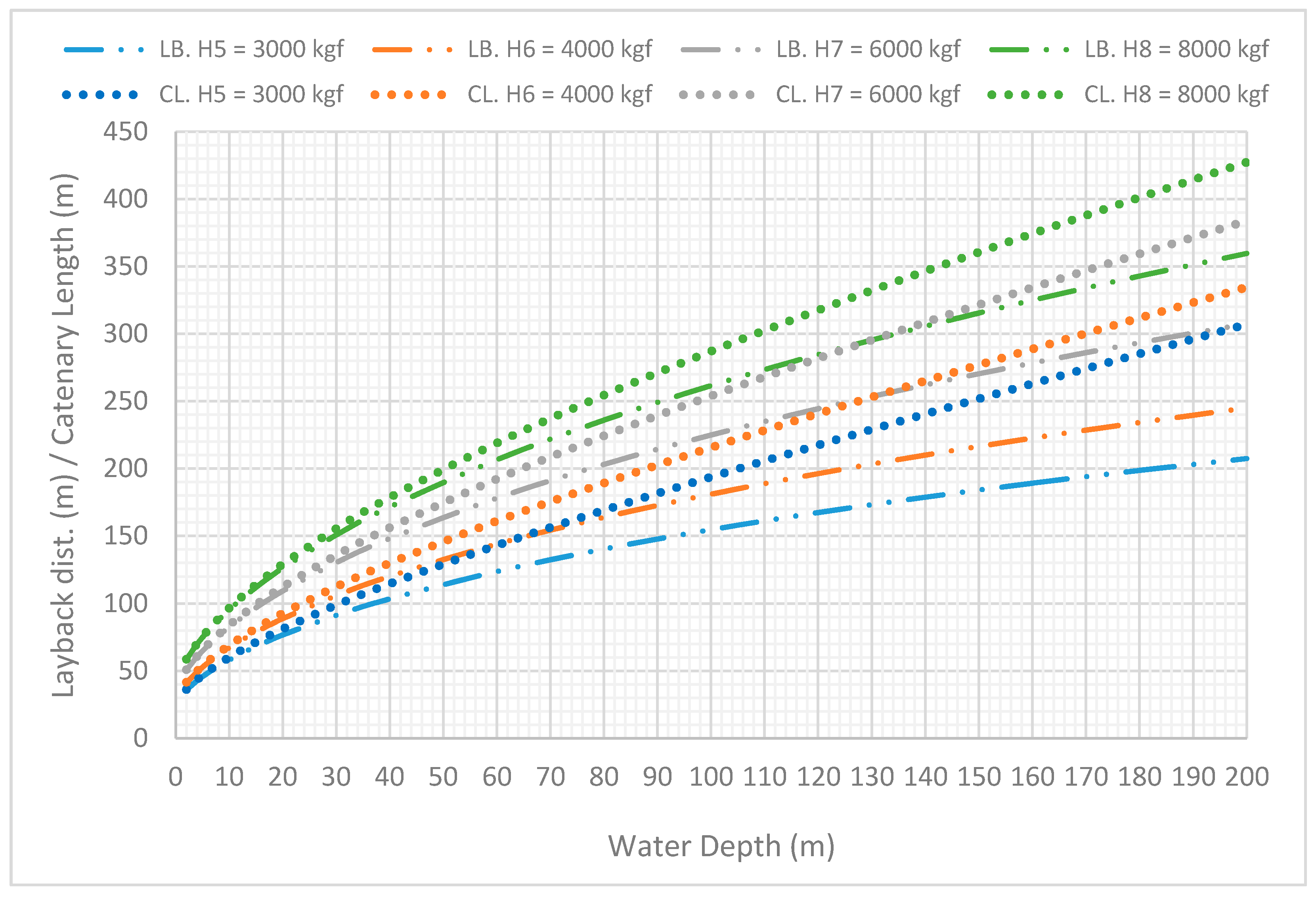
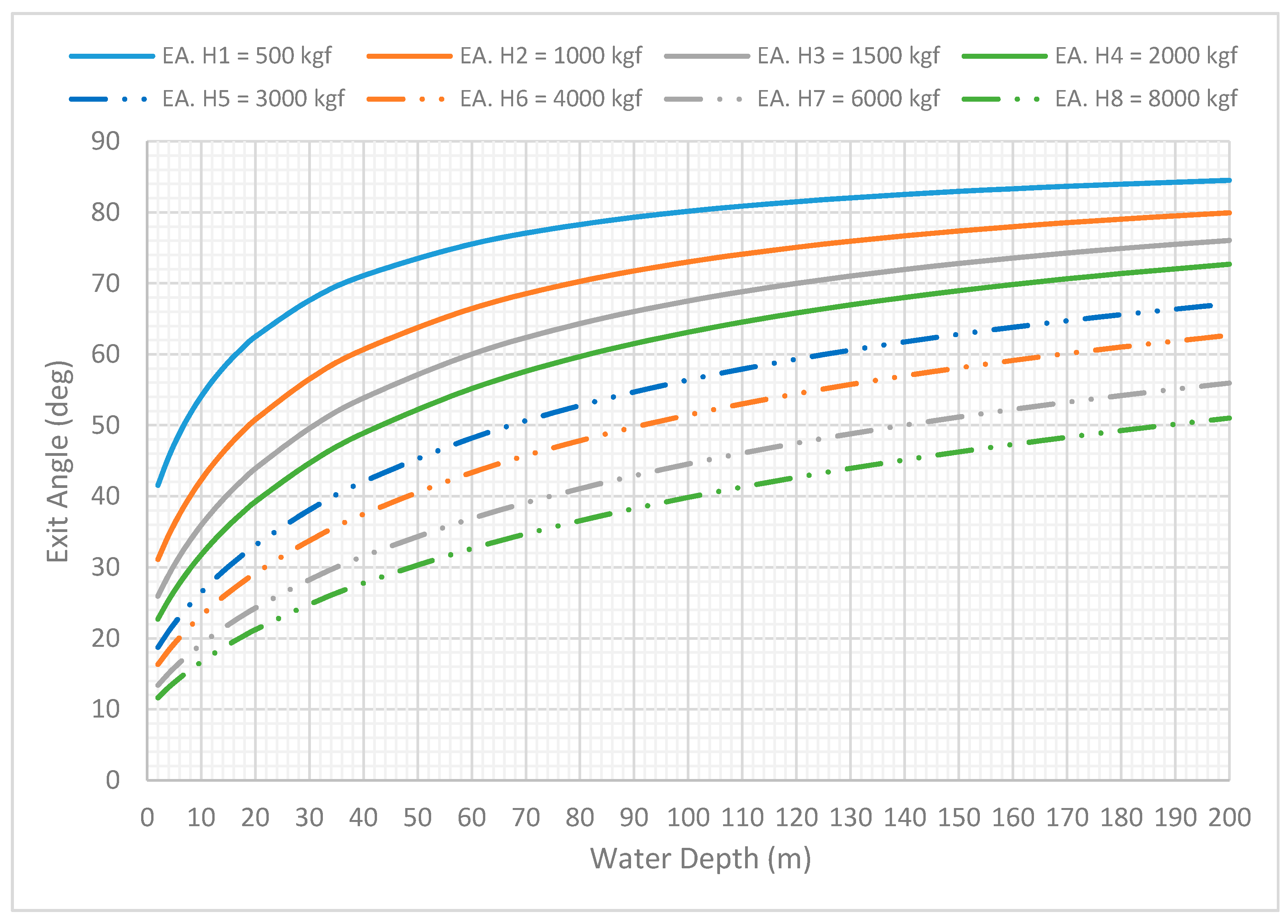
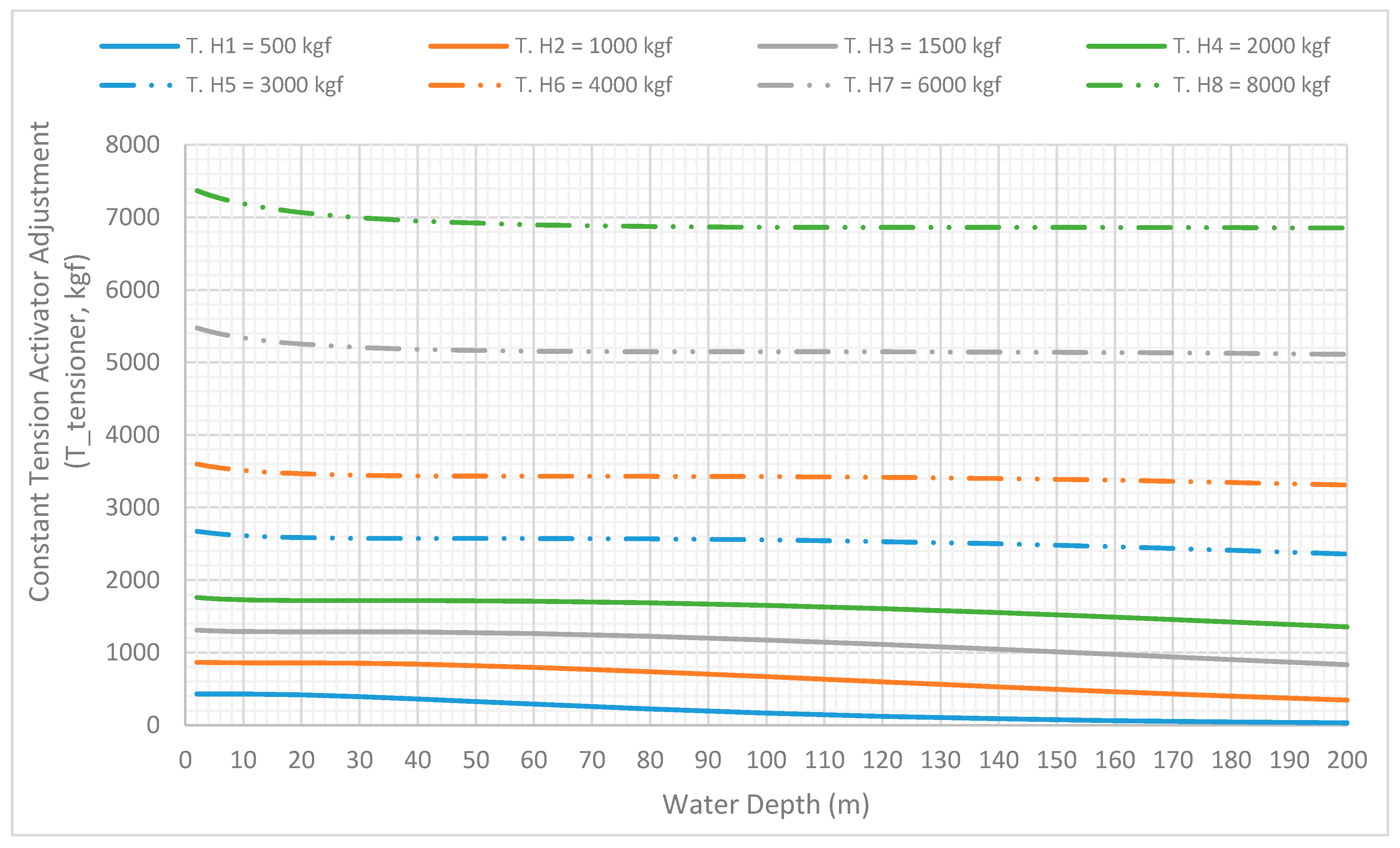
Analyzing different cable lay installation scenarios using a constant bottom tension varying between 500 kgf and 8000 kgf at different water depths, the main findings can be briefly concluded as follows. Layback distance (LB) and catenary length (CL) are increased as the water depth is increased. As the bottom tension is increased, the difference between the layback and catenary length for a specific water depth is decreased because the sag curve of the catenary configuration is becoming smoother. Exit angle (θ) is increased as the water depth is increased, meaning that the exit of the cable from the overboard chute is becoming steeper as the water depth is increased. Constant tension adjustment (T_tensioner) is decreased slightly as the water depth is increased. 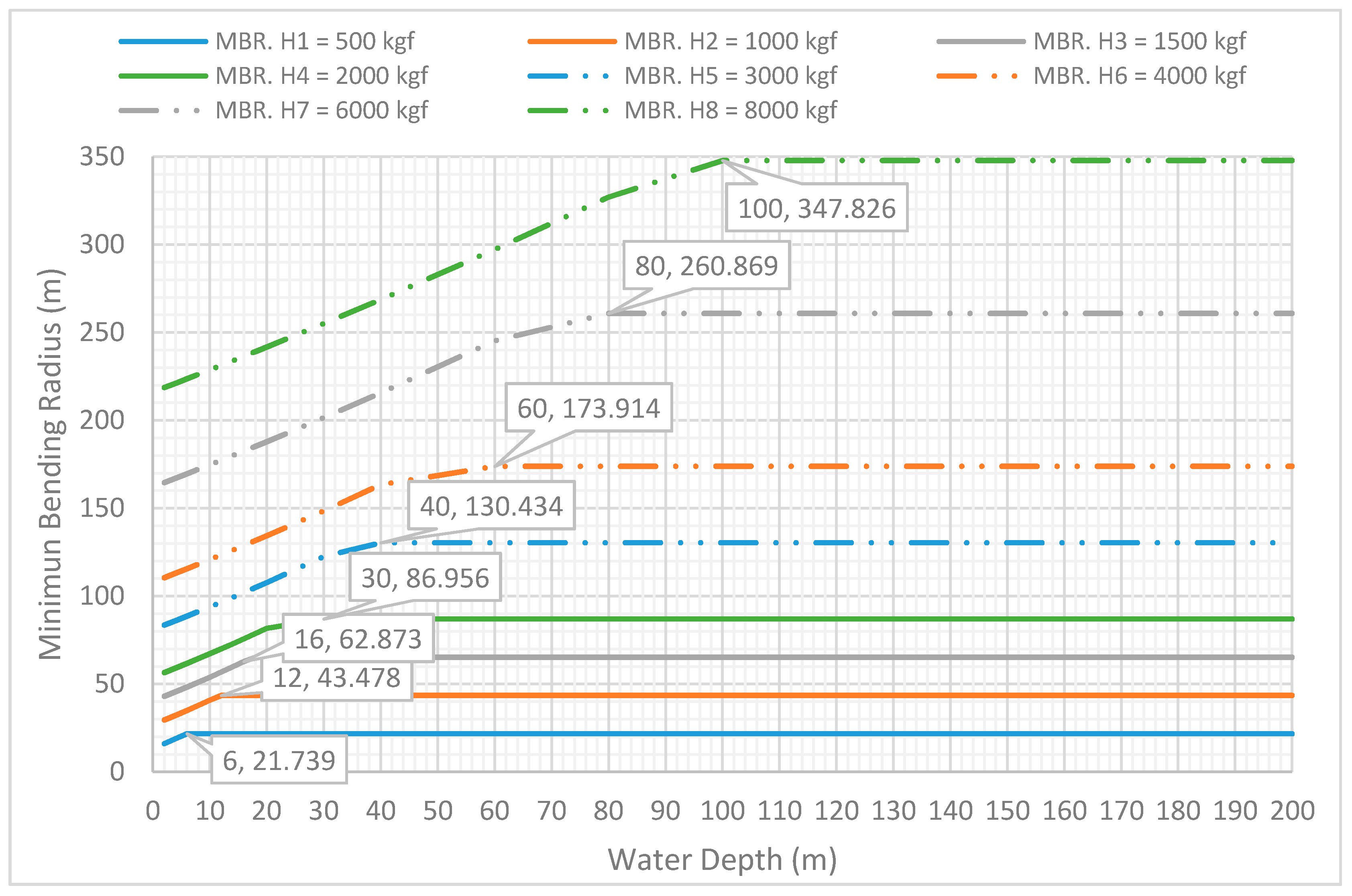The reason is that due to the increased exit angle, the friction forces [25] created by the contact between cable and overboard chute are increased and this results to less tension requirement by the tension machine to achieve the desired bottom tension. Minimum bending radius (= safety factor during installation) is increased as the water depth is increased up to the depth of 6 m (for 500 kgf) and 100 m (for 8000 kgf). After this depth, the minimum bending radius remains constant. The reason of this observation can be explained by analysing the actual bending radius Equation (1).

$$R=\frac{{[1+{(\sinh \left(\frac{q\ast x}{H}\right))}^2]}^{\frac{3}{2}}}{\frac{q}{H}\ast \cosh \left(\frac{q\ast x}{H}\right)},$$

(1)

For the submerged catenary curve, the minimum bending radius is located at the touch down point where x = 0 and the relevant Equation (1) can be expressed as (2). Therefore, for a specific bottom tension value, the minimum bending radius is constant if the minimum bending radius is located at the submerged part of the combined catenary curve.

$$MB{R}_{sub}=\frac{H}{q1},$$

(2)

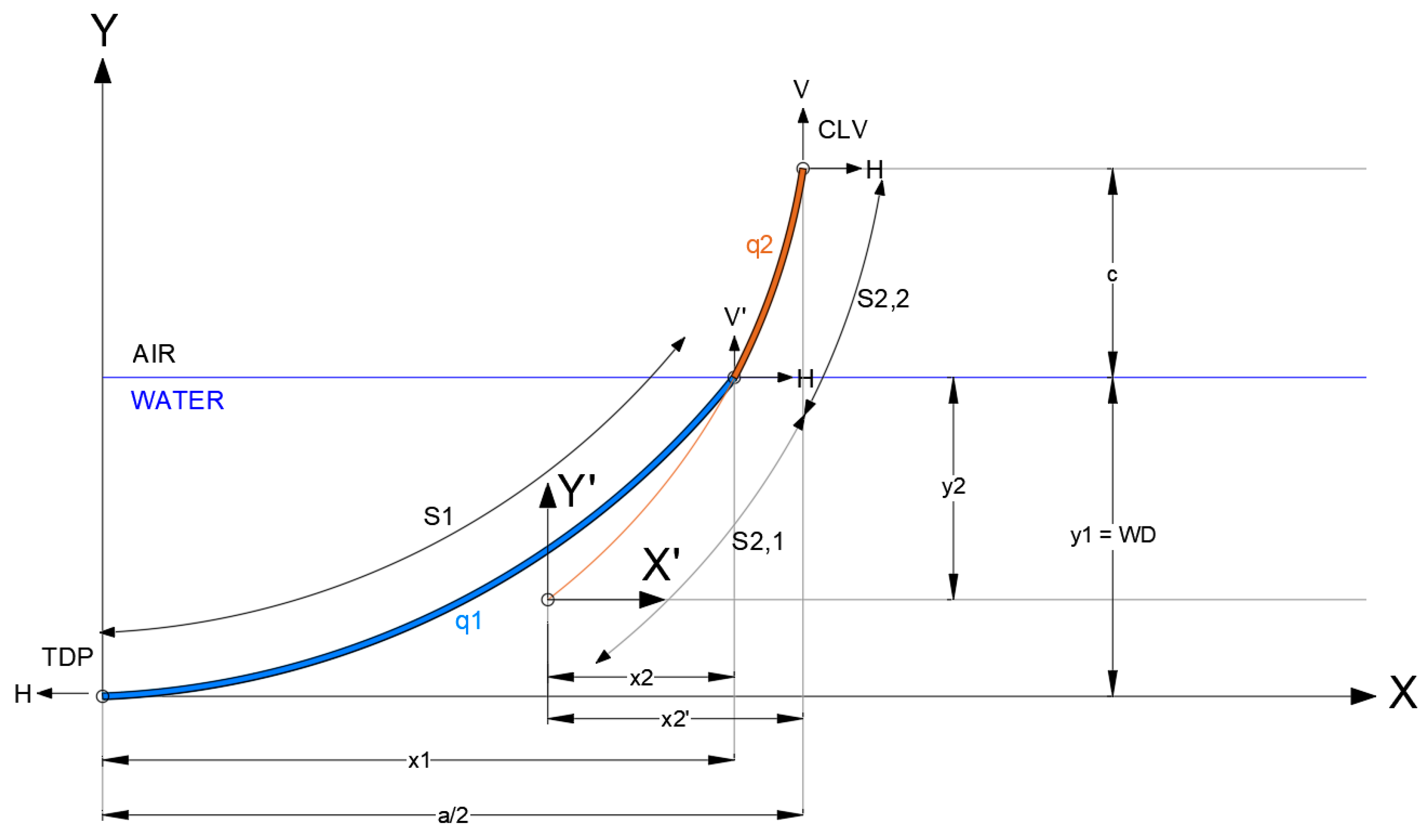
For the catenary curve in air, the minimum bending radius is located at the sea surface (air/water interface) where x = x2 (Figure 2). This location is varying depending on the specific (a) water depth and (b) bottom tension value. In order to determine how the actual bending radius for the catenary curve in air is varying, the Equation (1) will be expressed in a simpler way as (3).

$$MB{R}_{air}=\frac{H}{q2}\ast (\frac{TERM 1}{TERM 2}),$$

(3)

$$TERM 1={[1+{(\sinh \left(\frac{q2\ast x2}{H}\right))}^2]}^{\frac{3}{2}},$$

$$TERM 2=\cosh (\frac{q2\ast x2}{H}),$$

The value of x2 is increased as the water depth is increased. The quotient (TERM 1/TERM 2) is increased as the water depth is increased for a specific bottom tension value. Therefore, for a specific bottom tension value, the minimum bending radius is variable and increased as the water depth is increased if the minimum bending radius is located at the part in air of the combined catenary curve. In conclusion, the minimum bending radius is variable with the water depth in case it is located at the catenary curve in air (minimum value at the air/water interface) and in contrast the minimum bending radius is constant in case it is located at the submerged part (minimum value at the TDP). Thus, as per Table 2 and Table 3 results, the water depth of 6 m and 100 m is the critical water depth for the bottom tension of 500 kgf and 8000 kgf respectively where the minimum bending radius is defined by the submerged part (located at the TDP) and becomes constant for deeper areas assuming the specific bottom tension.

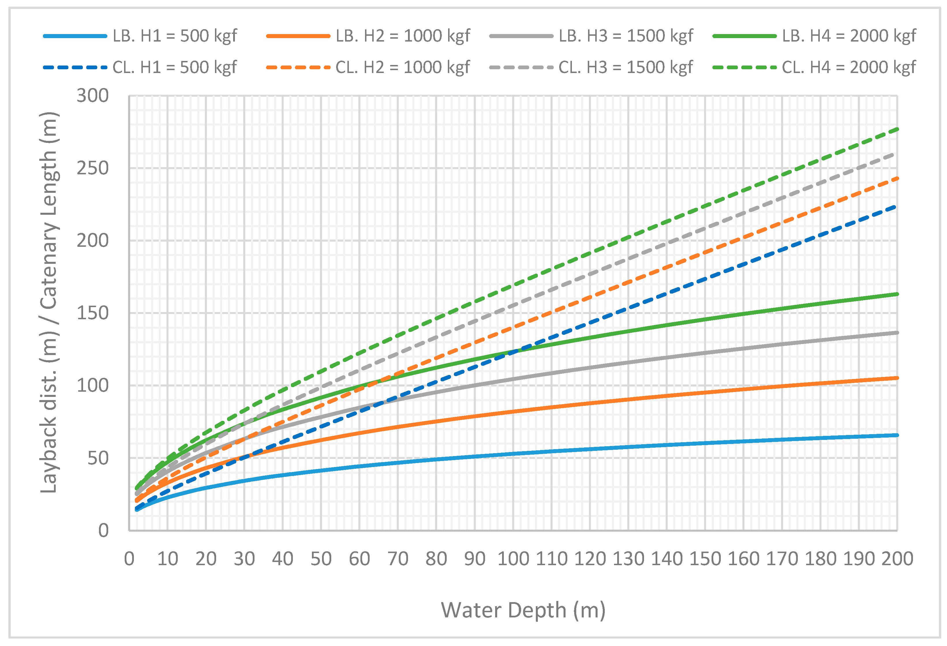
Different installation parameters during a cable deployment process using various bottom tension values and water depths are illustrated in Figure 4, Figure 5, Figure 6, Figure 7 and Figure 8. The layback distance (LB) and catenary length (CL) are presented in Figure 4 and Figure 5 for bottom tensions 500 kgf–2000 kgf and 3000 kgf–8000 kgf, respectively. The exit angle (θ), minimum bending radius (MBR) and the constant tension activator adjustment (T_tensioner) are presented in Figure 6, Figure 7 and Figure 8, respectively.

The parametric study presented above can be summarized by pointing out the following key rules. Layback distance (LB) and catenary length (CL) are increased as the water depth is increased (assuming constant bottom tension). Layback distance (LB) and catenary length (CL) are increased as the bottom tension is increased (assuming constant water depth). Difference between layback distance (LB) and catenary length (CL) at the same water depth is decreasing progressively as the bottom tension value is increasing, since the catenary curve due to the increased axial tension tends to become a straight line minimizing the sag of the curve. Exit angle (θ) is increased as the water depth is increased (assuming constant bottom tension). Exit angle (θ) is decreased as the bottom tension is increased (assuming constant water depth). It should be noted that as the exit angle is increased, the length of the cable in contact with the overboard chute is increased and therefore the friction created is increased as well. Constant tension adjustment on the tension machine (T_tensioner) is decreased slightly as the water depth is increased. This is quite strange since the weight of the suspended cable during laying is increased as the water depth is increased and therefore the force required to be provided by the tensioner should have been increased as well to compensate the extra weight of the cable. However, the reason explaining this phenomenon is that due to the increased exit angle, the friction forces created by the contact between cable and overboard chute are increased and this results to less tension requirement by the tension machine to achieve the desired bottom tension. For the sake of installation easiness, the adjustment on the tension machine can be ignored if the water depth variation along the cable route is not so much, since the friction between cable and overboard chute is acting as a natural compensation of the cable suspended weight as the water depth is increased. Minimum bending radius (safety factor during laying) is increased as the bottom tension is increased and there is no upper limit (assuming constant water depth), as described by Equations (2) and (3). It must be reminded here that high bottom tension values increase the safety factor, however, special attention should be paid because this creates cable suspensions along uneven sea floors as a result of the restrained tension created by the friction between seabed and cable. Minimum bending radius (safety factor during laying) is increased as the water depth is increased and remains constant after a specific depth value according to the bottom tension (assuming constant bottom tension). As explained above, for each specific bottom tension value, a critical water depth can be numerically defined for which the minimum bending radius is derived by the submerged part and remains constant for every deeper area than the critical depth.

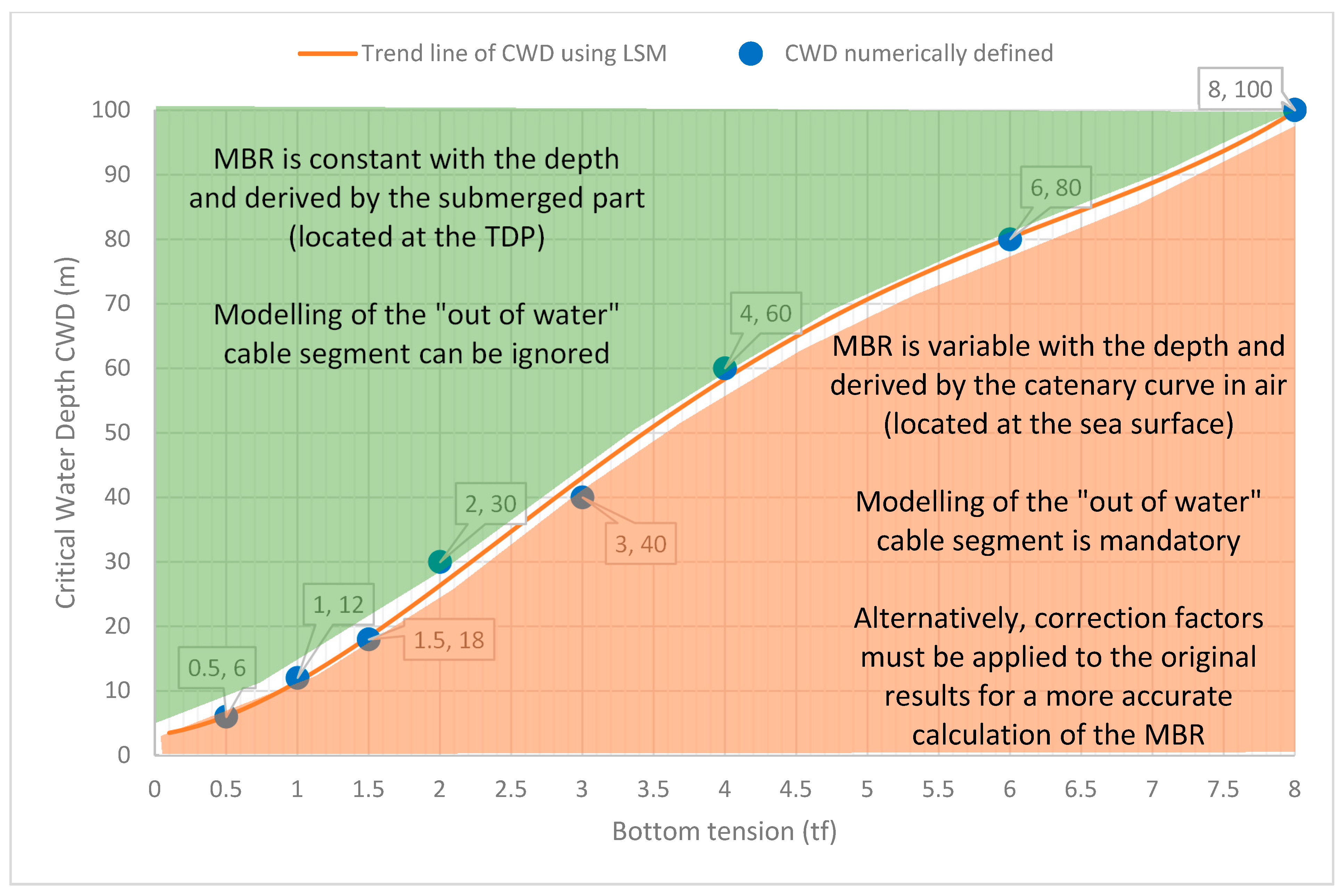
The critical water depth (CWD), numerically defined at the points where the combination of bottom tension and water depth is marked, is presented in Figure 9 using the blue scatters. The trend line of the CWD is numerically approximated using the least square method (LSM) and presented using the orange line. A fourth-degree polynomial equation is utilized in order to minimize the error of approximation for the numerical expression of the CWD and provided here below.

$$CWD=0.0698\ast H^4-1.2321\ast H^3+6.5376\ast H^2+2.9029\ast H+3.1488,$$

(4)

The Figure 9 in conjunction with Equation (4) can be used as guidance for all the cable installers in order to determine the cases which are critical for the modelling of the “out of water” cable segment. The combinations of bottom tension (H) and water depth (WD) that are located into the green area at the left-top part of the graph are those in which the MBR is constant as the water depth is further increased and is derived by the submerged part of the catenary curve. For these installation cases, the “out of water” cable segment can be ignored without denoting the accuracy of the MBR calculation. In contrast, the combinations of bottom tension (H) and water depth (WD) that are located into the red area at the right-bottom part of the graph are those in which the MBR is variable as the water depth is further decreased and is derived by the part of catenary curve in air. For these installation cases, the combined catenary curve must be calculated as described in the present paper. Alternatively, the cable installers should apply the correction factors which are proposed in the next section to the original results in order to improve the accuracy of the actual MBR calculation.

3.2. Influence for the Modelling of the “Out of Water” Cable Segment

The effect of the “out of water” cable segment, the part of cable between the sea surface and the cable ship overboard chute, has been investigated especially for shallow water applications. Utilizing the installation curves and the correction factors provided in the present paper, corrections can be conducted when cable responses do not include the “out of water” cable segment.

Evaluation of the influence for the modelling of the cable part in air will be conducted comparing two different case studies (CS). The modelling of the combined catenary curve, assuming “submerged” the part between the touch down point to the sea surface and “in air” the part between the sea surface and the last point touching the overboard chute on the cable lay vessel, is named as CS1. In contrary, the modelling of the submerged catenary curve, assuming “submerged” the whole length of the suspended cable between the touch down point and the last point on the overboard chute, is named as CS2. Both the case studies have been analyzed assuming different water depth values starting from 2 m water depth and ending at 20 m water. Furthermore, as bottom tension input, two different set of 4 runs were conducted assuming as first set the values of 500/1000/1500/2000 kgf and as second set the values of 3000/4000/6000/8000 kgf. The friction force between cable and overboard chute is calculated for both case studies using the capstan equation [25] and the friction coefficient is assumed equal to μ = 0.5.

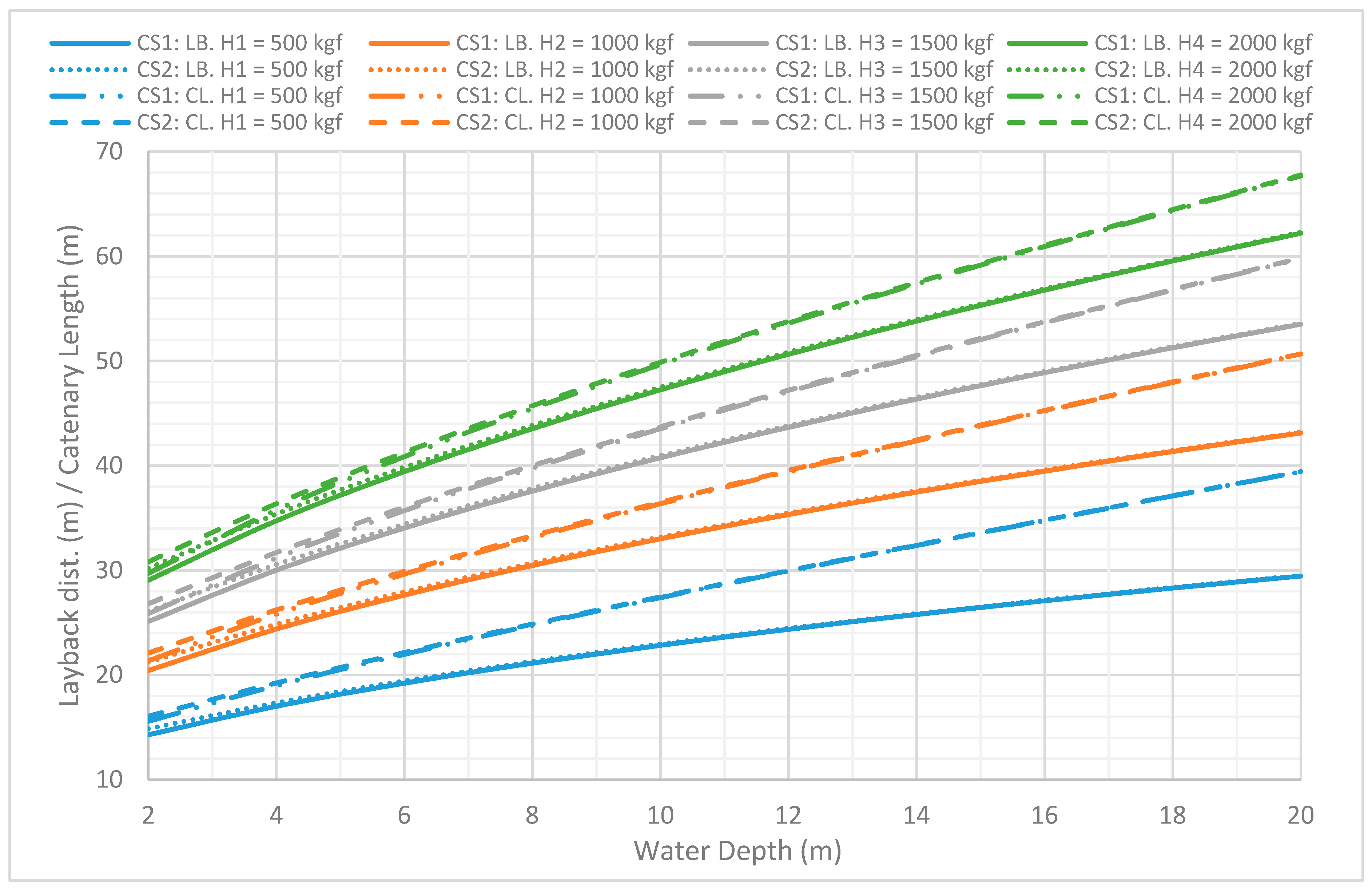
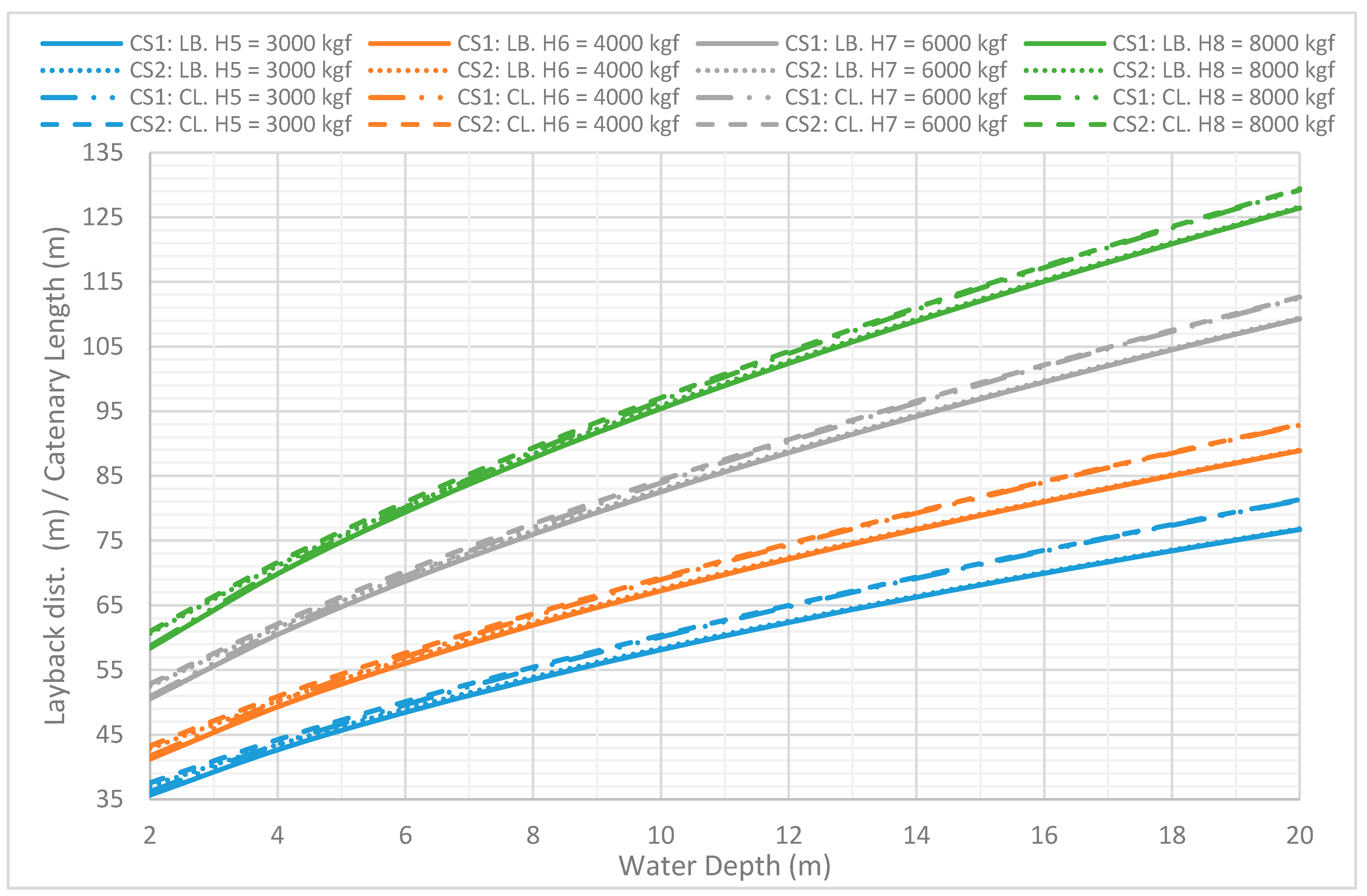
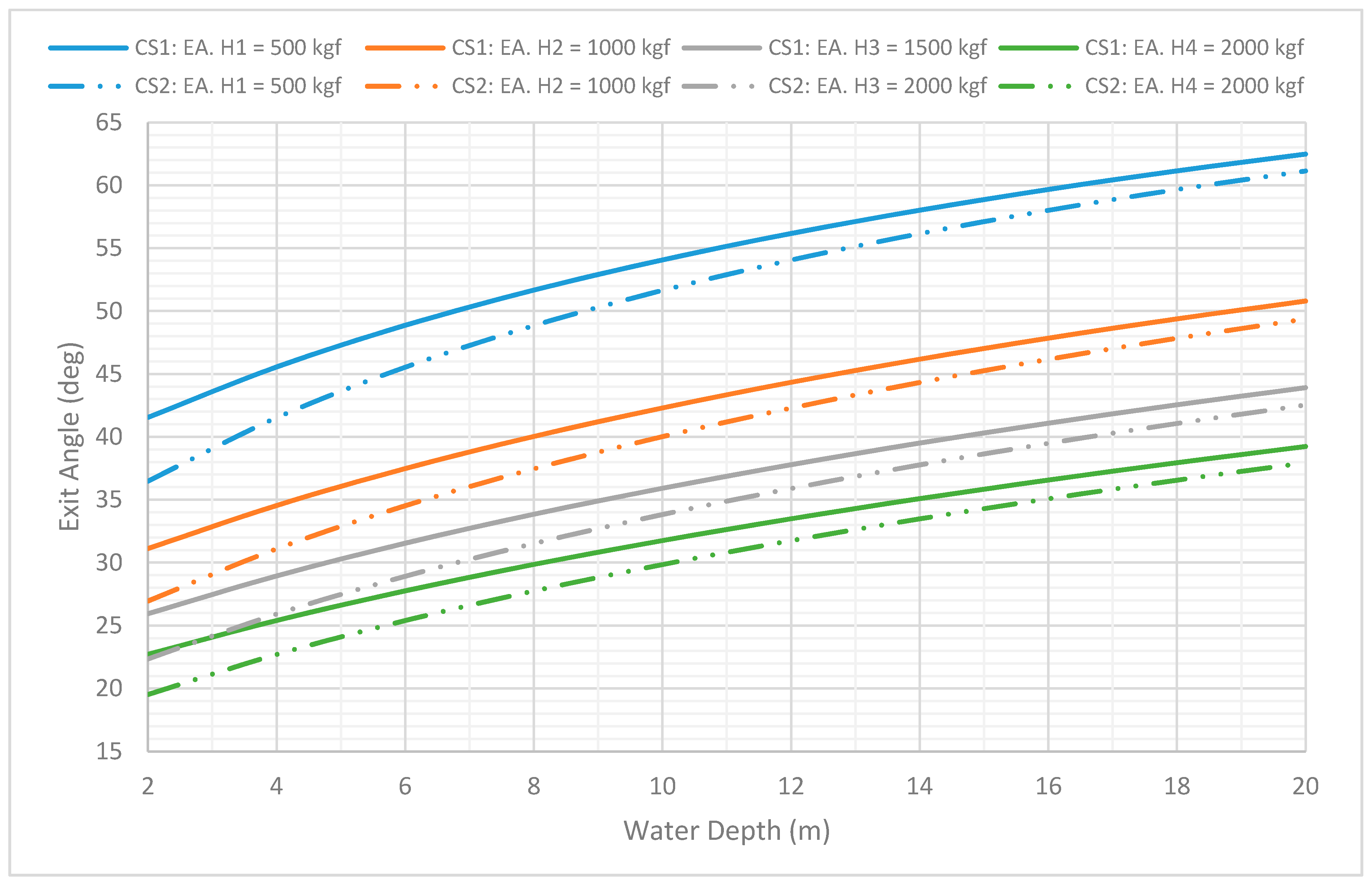
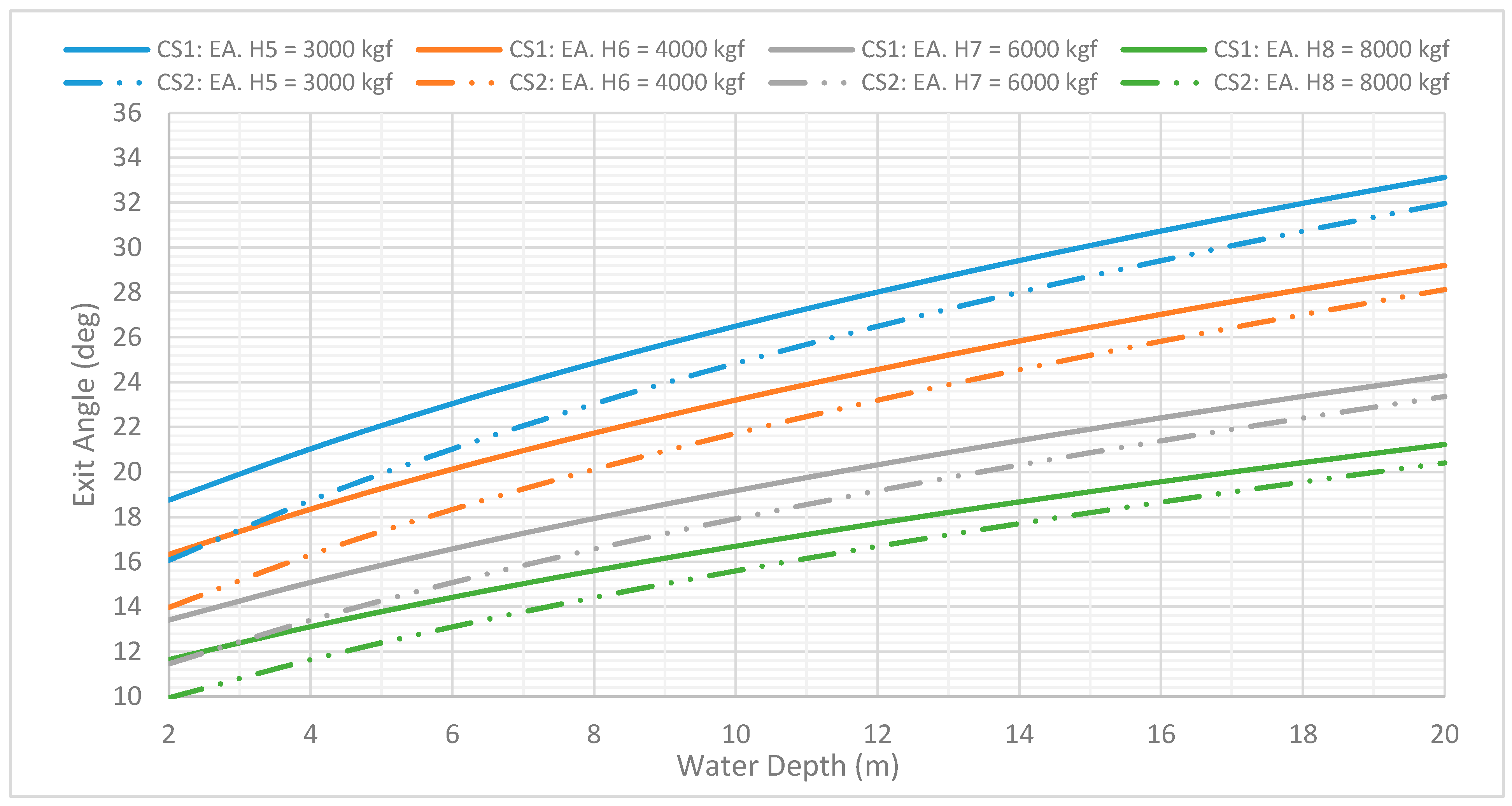
Different cable critical responses during a cable deployment process using various bottom tension values and water depths are illustrated in Figure 10, Figure 11, Figure 12, Figure 13, Figure 14 and Figure 15 for both case studies CS1 and CS2. The layback distance (LB) and catenary length (CL) are presented in Figure 10 and Figure 11 for bottom tensions 500 kgf–2000 kgf and 3000 kgf–8000 kgf, respectively. 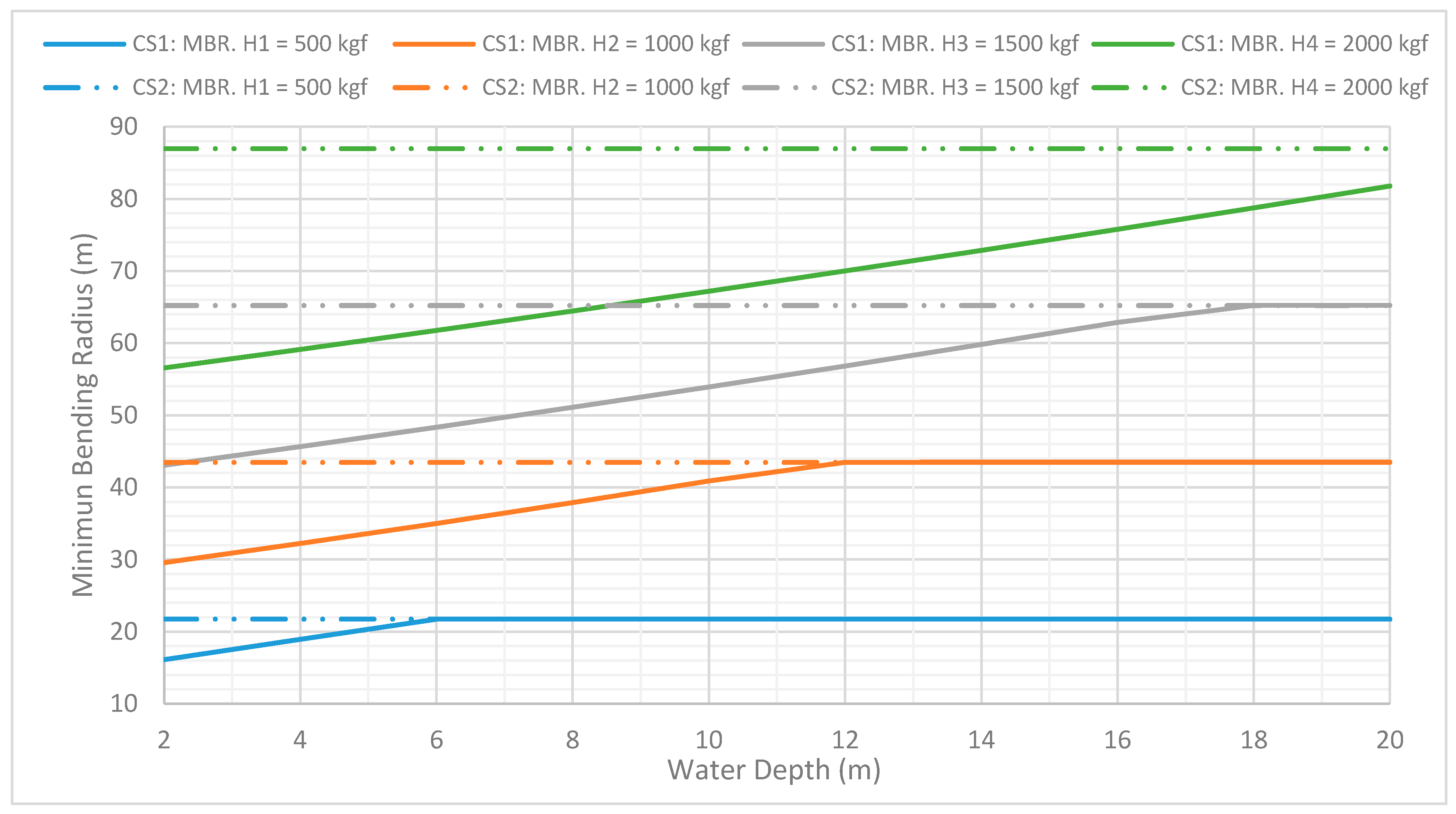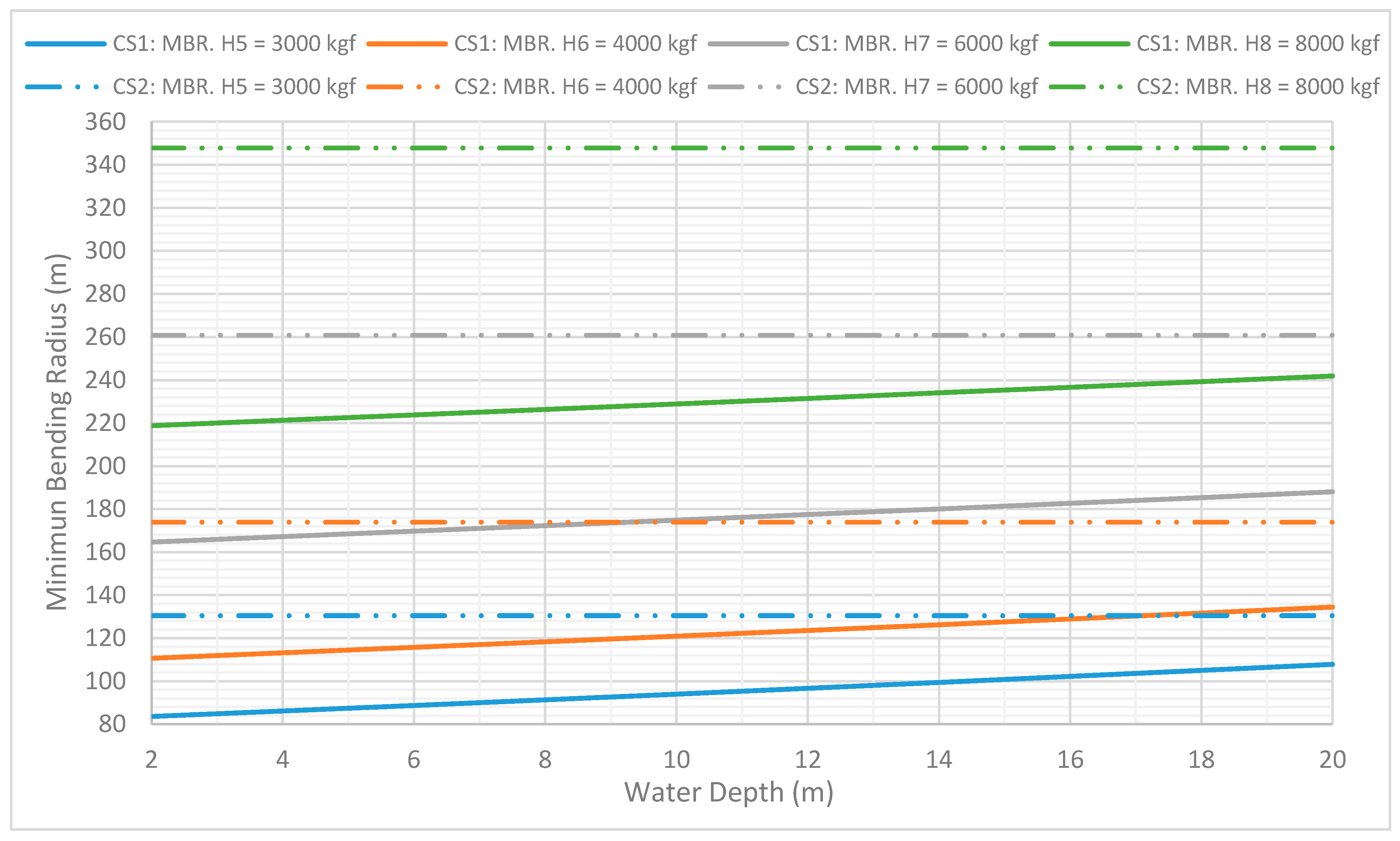The exit angle (θ) is presented in Figure 12 and Figure 13 for bottom tensions 500 kgf–2000 kgf and 3000 kgf–8000 kgf, respectively. The minimum bending radius (MBR) is presented in Figure 14 and Figure 15 for bottom tensions 500 kgf–2000 kgf and 3000 kgf–8000 kgf, respectively.

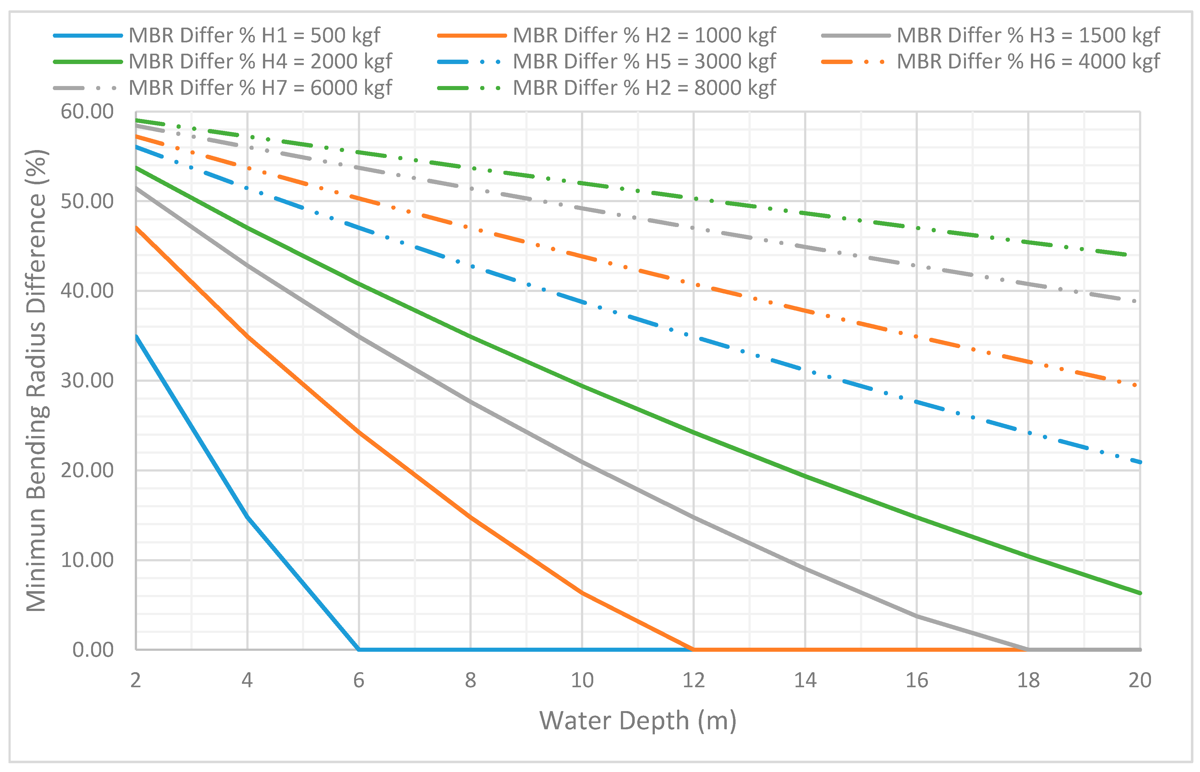
The study presented above for the evaluation of the influence for the modelling of the “out of water” cable segment can be summarized by pointing out the following key rules. Layback distance (LB) is not influenced significantly by the modelling or not of the “out of water” cable segment. The maximum difference between CS1 and CS2 is presented in shallow waters and is equal to 4.15%. The variation of the difference between the two case studies when the bottom tension is varying between 500 kgf–8000 kgf is ignorable and equal to 4.15–3.92% respectively. This difference is decreased as the water depth is increased. Catenary length (CL) is not influenced significantly by the modelling or not of the “out of water” cable segment. The maximum difference is presented in shallow waters and is equal to 3.85%. The variation of the difference between the two case studies when the bottom tension is varying between 500 kgf–8000 kgf is ignorable and equal to 3.16–3.85% respectively. This difference is decreased as the water depth is increased. Cable exit angle (θ) is influenced by the modelling of the “out of water” cable segment. The maximum difference is presented in shallow waters and is equal to 14.63%. The variation of the difference between the two case studies when the bottom tension is varying between 500 kgf–8000 kgf is equal to 12.18–14.63% respectively. This difference is decreased as the water depth is increased. At the maximum water depth (20 m) that the present study was conducted, the difference is almost ignorable and equal to 3.84%. Minimum bending radius (safety factor during cable laying operation) is significantly influenced by the modelling of the “out of water” cable segment as the bottom tension value is increased. As the bottom tension value is increased, the cable exit angle is decreased and the length of the cable segment which is “out of water” is longer, thus the influence of this part is becoming more significant to the system response. The maximum difference is present in shallow water area and is equal to 59.04% at the maximum bottom tension value of 8000 kgf. The variation of the difference between the two case studies when the bottom tension is varying between 500 kgf–8000 kgf is equal to 34.92–59.04% respectively. This difference is decreased as the water depth is increased. At the maximum water depth (20 m) that the present study was conducted, the difference between the two case studies when the bottom tension is varying between 500 kgf–8000 kgf is equal to 0.00–43.85% respectively. It should be noted that for the low values of bottom tension (500 kgf–1500 kgf), there is no difference between the CS1 and CS2 for water depths deeper than the relevant critical water depth. This proves the theory of the critical water depth as presented and described in Figure 9. Minimum bending radius difference (%) between the two case studies is presented in

Table 4. MBR difference (%) comparing CS1 & CS2 using different bottom tensions (500 kgf–8000 kgf) and water depths (2 m–20 m).

Water Depth (m)	MBR Difference %
	H1 500 kgf	H2 1000 kgf	H3 1500 kgf	H4 2000 kgf	H5 3000 kgf	H6 4000 kgf	H7 6000 kgf	H8 8000 kgf
2	34.92	47.03	51.44	53.72	56.05	57.23	58.43	59.04
4	14.78	34.92	42.82	47.04	51.44	53.72	56.05	57.24
6	0	24.23	34.91	40.78	47.03	50.32	53.72	55.46
8	0	14.75	27.64	34.91	42.81	47.03	51.44	53.72
10	0	6.34	20.94	29.40	38.78	43.85	49.21	52.01
12	0	0	14.76	24.22	34.91	40.77	47.03	50.32
14	0	0	9.03	19.35	31.19	37.79	44.90	48.66
16	0	0	3.73	14.75	27.63	34.90	42.81	47.03
18	0	0	0	10.42	24.22	32.11	40.77	45.43
20	0	0	0	6.33	20.94	29.40	38.77	43.85

and illustrated in Figure 16 because is the most crucial parameter for the cable integrity during the deployment process. It should be noted that the minimum bending radius for the specific subsea cable that is used in this study is much bigger than the minimum allowable recommended by the manufacturer (MBR_actual = 16.11 m >> MBR_{min.allowable} = 2.2 m) even if the “out of water” cable segment has been taken into consideration. However, the 59% analysis error on the MBR quantification deserves attention to be get for the deployment cases of more sensitive in bending stresses cables and pipelines.

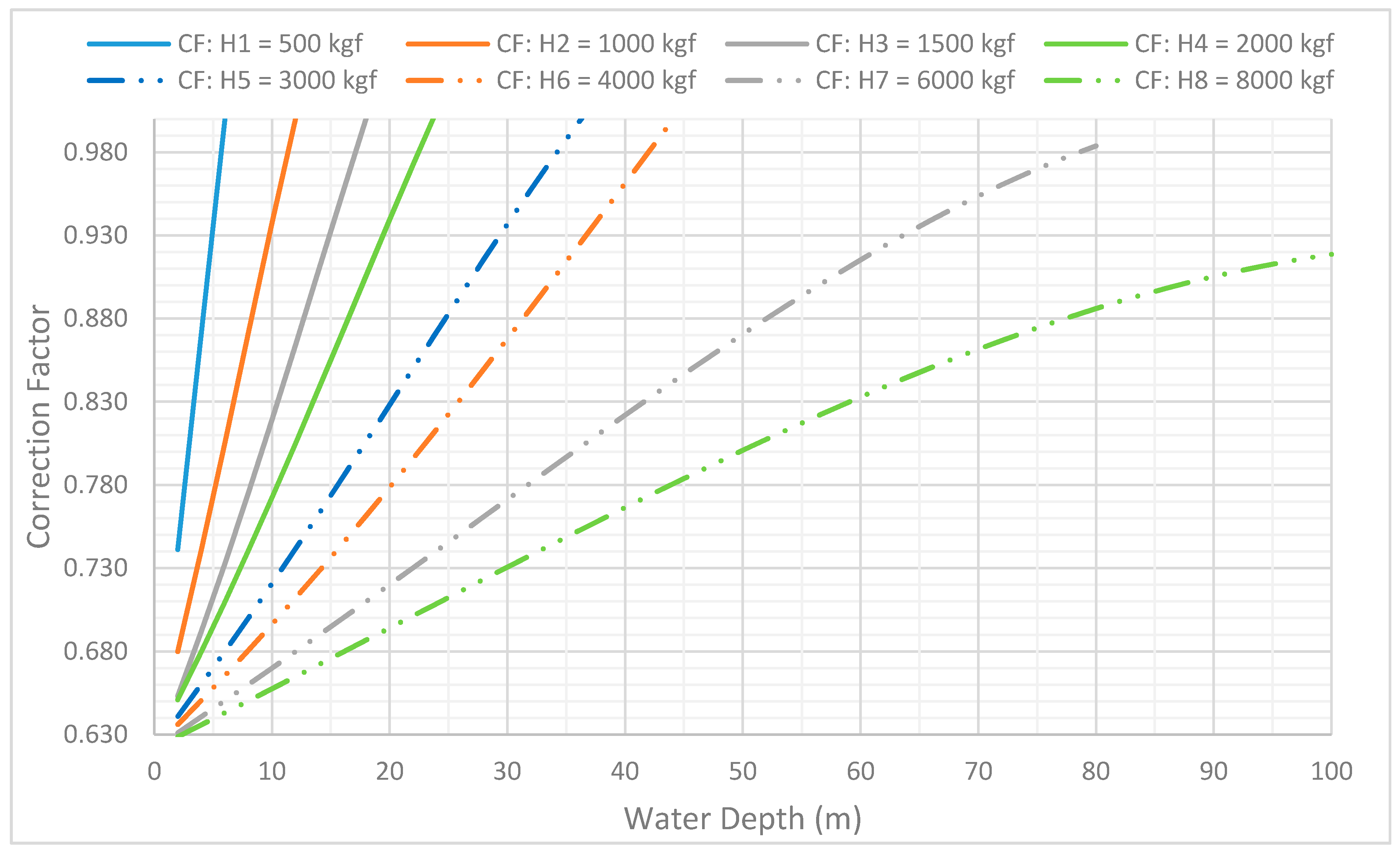
Processing the results of the above presented study, multiplying correction factors (CF) are proposed for various bottom tension (H) and water depth (WD) combinations in order to allow the cable installers to improve the calculation accuracy of the minimum bending radius in case of not modelling the “out of water” cable segment. Analytical expressions of correction factors for different values of bottom tensions (H) are presented here after. Correction factors are valid only for combinations of bottom tension and water depth which are laid into the red area of Figure 9.

$$CF=\{\begin{array}{cc}\frac{1}{E{q}_H+1},& WD<CWD\\ 1 ,& WD\ge CWD\end{array} ,$$

(5)

$$E{q}_H=0.0067\ast W{D}^2-0.1409\ast WD+0.6041 , for H=500 kgf$$

$$E{q}_H=0.0017\ast W{D}^2-0.0709\ast WD+0.6058 , for H=1000 kgf$$

$$E{q}_H=0.0007\ast W{D}^2-0.0472\ast WD+0.6057 , for H=1500 kgf$$

$$E{q}_H=0.0004\ast W{D}^2-0.035\ast WD+0.6046 , for H=2000 kgf$$

$$E{q}_H=0.0002\ast W{D}^2-0.024\ast WD+0.6073 , for H=3000 kgf$$

$$E{q}_H=0.0001\ast W{D}^2-0.0182\ast WD+0.6081 , for H=4000 kgf$$

$$E{q}_H=0.00006\ast W{D}^2-0.0122\ast WD+0.6085 , for H=6000 kgf$$

$$E{q}_H=0.00004\ast W{D}^2-0.0092\ast WD+0.6086 , for H=8000 kgf$$

As illustrated in Figure 17, multiplying correction factors are varying between 0.629 and 1.0. For intermediate values of bottom tension (H), linear interpolation can be applied to estimate the correction factor. For example, a cable laying operation is taken place at a water depth of 10 m with a bottom tension of 2000 kgf. The minimum bending radius calculated by the analysis tool ignoring the “out of water” cable segment is 86.96 m. As per Figure 17, the corrective factor corresponds to this combination is 0.772. Thus, multiplying the original value of 86.96 m with the corrective factor of 0.772, the corrected value of the MBR is 67.13 m. It should be noted that the relevant value of the MBR analysing the combined catenary curve is 67.19 m. Therefore, even if the cable installers are not able to analyse a combined catenary curve, now they are able to use the proposed correction factors in order to improve the accuracy of the MBR calculation.

3.3. Overboard Cable Chute Friction Modelling Effects

When the submarine cables are laid from the overboard chute of a cable laying vessel, there are the following components that contribute to the axial forces along the submarine cable. Gravity forces by the submarine cable self-weight, buoyancy forces, residual desired bottom tension on the seabed, drag and inertia forces due to the hydrodynamic loads created by currents, waves, and cable ship motions. Thus, as already presented in [4,6,8,9,10,11,14,15,16,17,18], practical cable tension at ship “T_tensioner” can be written, after a slight modification to include the “out of water” cable segment, as:

$$T_{tensioner}=\left(q1\ast WD+q2\ast c\right)+H\pm T_{dyn}$$

(6)

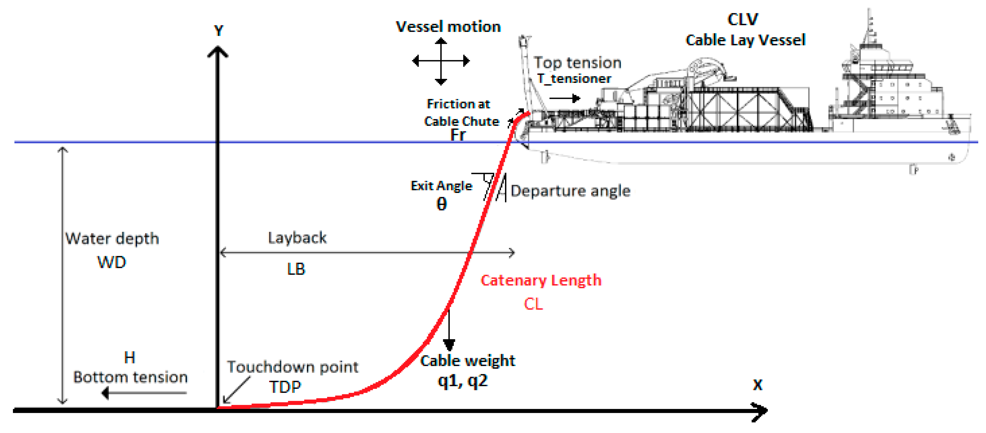
“T_tensioner” is the tension machine adjustment in terms of force units onboard the cable laying vessel. This is the only parameter that can be monitored real time by the cable installers with the common available equipment nowadays in the cable industry. The cable self-weight is expressed as “q1” for the submerged part and as “q2” for the “out of water” cable segment. “WD” is the water depth at the touch down point and “c” is the vertical distance between the sea surface and the last touching point of the cable on the overboard chute. “H” is the desired residual bottom tension of the cable on the seabed. “T_dyn” is the effect of the hydrodynamic loads due to currents, wave, cable ship motions and asynchronization between cable ship velocity and cable pay-out rate on the axial force along the cable. However, there is one more component that is hidden in this equation and can play a major role in the cable laying analysis. This component is the friction force created by the contact between the cable and the overboard chute and can change dramatically the equilibrium of the forces acting on the cable having positive or negative consequences in case of inaccurate modelling. The in-house cable analysis model is further developed using analytical equations for the calculation of the friction force introduced by the contact between cable and chute. Therefore, the equation that is used by the proposed analysis tool and describes the practical cable tension at ship “T_tensioner” has been extended to account for the friction forces on the cable chute as follows:

$$T_{tensioner}=\left(q1\ast WD+q2\ast c\right)+H\pm T_{dyn}\pm \mathrm{Fr}$$

(7)

The “Fr” is the friction forces created by the contact between cable and overboard chute of the cable ship. Sign “+” is valid for the cable recovery operations and sign “−“ is valid for the laying operations. Cable recovery is a critical operation in that tension requirements by the onboard tensioners can be significantly higher than those encountered during installation.

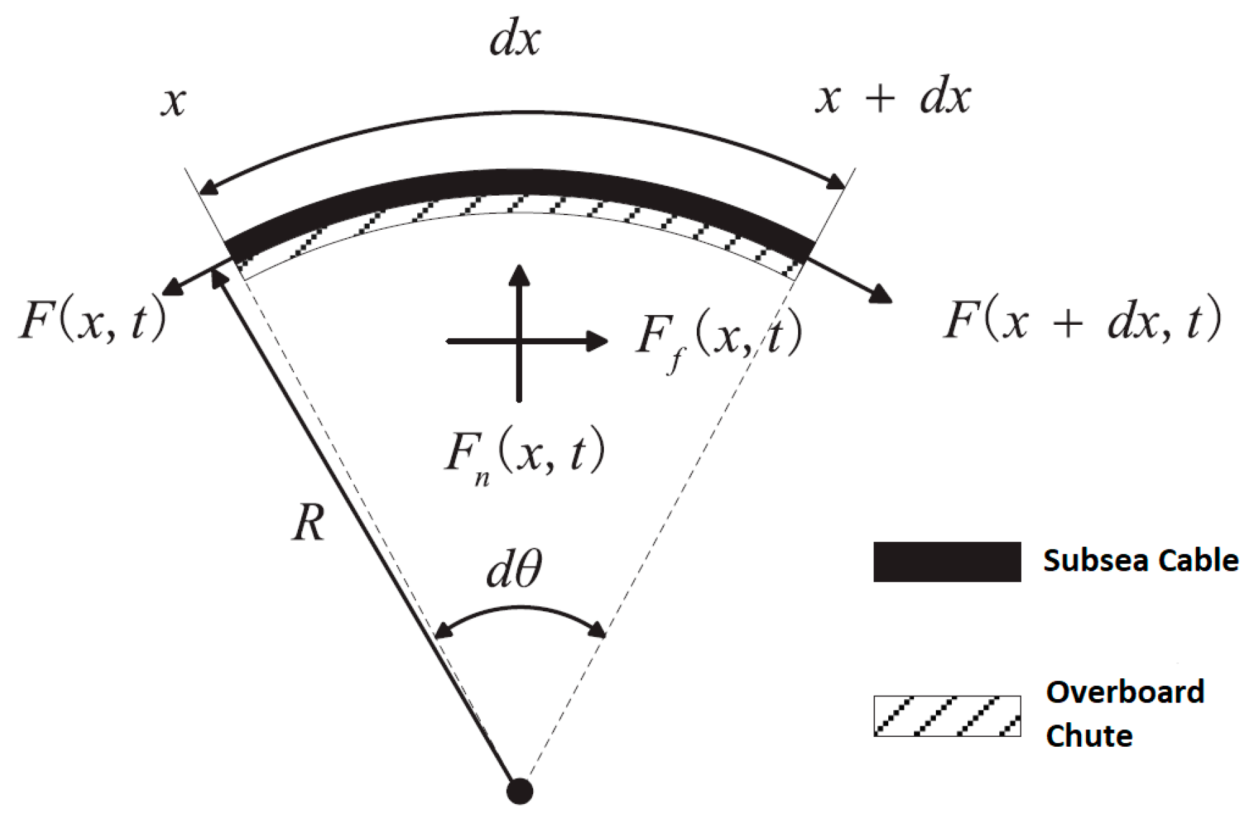
The friction between cable and sliding surface of the overboard chute is mainly due to the tension exerted on both ends of cable, just before the chute by the tensioner and after the chute by the suspended part of cable. The force analysis of cable infinitesimal is about to be described [27]. As shown in Figure 18, the direction of force transferring is left-to-right along the overboard chute sliding surface of the radius R. The relative sliding happens between cable and sliding surface, and the stress analysis of the cable infinitesimal is carried out as follows:

$$F_n\left(x,t\right)=F\left(x,t\right)\ast \sin \left(\frac{d\theta }{2}\right)+F\left(x+dx, t\right)\ast \sin \left(\frac{d\theta }{2}\right)$$

(8a)

$$sign\left(v\right)\ast F_f\left(x,t\right)=F\left(x,t\right)\ast \cos \left(\frac{d\theta }{2}\right)-F\left(x+dx, t\right)\ast \cos \left(\frac{d\theta }{2}\right)$$

(8b)

$$dF\left(x,t\right)=F\left(x+dx,t\right)-F\left(x, t\right)$$

(8c)

$$F_f\left(x,t\right)=\mu \ast F_n\left(x,t\right)$$

(8d)

where “dθ” is the wrap angle between the cable infinitesimal element and the sliding surface of the overboard chute, “dx” is the arc length of the cable infinitesimal element, “F(x, t)”, “F(x + dx, t)” are the tension of the cable infinitesimal element initiator and terminal at time t. For typical cable laying activities, initiator is the tensioner side and terminal is the suspended cable side (out of the vessel) and vice versa for a cable recovery operation. “dF(x, t)” is the tension difference between the initiator and the terminal of the cable infinitesimal element at time t, “v” is the cable velocity along the overboard chute, “F_n(x, t)” is the normal support force of the cable from the overboard chute at the time t, and “F_f(x, t)” is the Coulomb friction resulting from the relative motion between the cable and the sliding chute at the time t. Therefore, the friction model for the calculation of the friction force created by the contact between cable and overboard chute can be expressed as:

$$F\left(x,t\right)=F\left(0,t\right)\ast e^{\left[-sign\left(v\right)\ast \mu \ast \theta \right]}$$

(9a)

$$Fr=F\left(x,t\right)-F\left(0,t\right)=e^{\left[-sign\left(v\right)\ast \mu \ast \theta \right]}$$

(9b)

where “θ” is the wrap angle between the cable and the sliding surface of the overboard chute, “μ” is the friction coefficient, “F(0, t)” is the tension of cable initiator at time t, “F(x, t)” is the cable tension at the x away from the initiator at time t, sign(v) is the sign of the cable velocity for which the sign “−“ is assumed for typical cable laying activities and sign “+” for cable recovery activities and “Fr” is the tension difference between initiator and terminal which is inserted as the friction component in Equation (7). From Equation (9a) is proven that the friction between cable and the overboard chute just depends on the friction coefficient “μ” and the wrap angle “θ” and is irrelevant to the routing radius “R” of the cable along the sliding surface of the cable chute or the area of contact.

The friction model presented above has been incorporated in the custom-made cable analysis tool [24] and the extended Equation (7), proposed in the present paper, is adopted for the calculation of the cable tension at ship (T_tensioner). A brief presentation of the core equations is provided to explain how the proposed friction model has been accounted for in the in-house analysis tool. Further details about the full numerical model can been found in the reference paper [24].

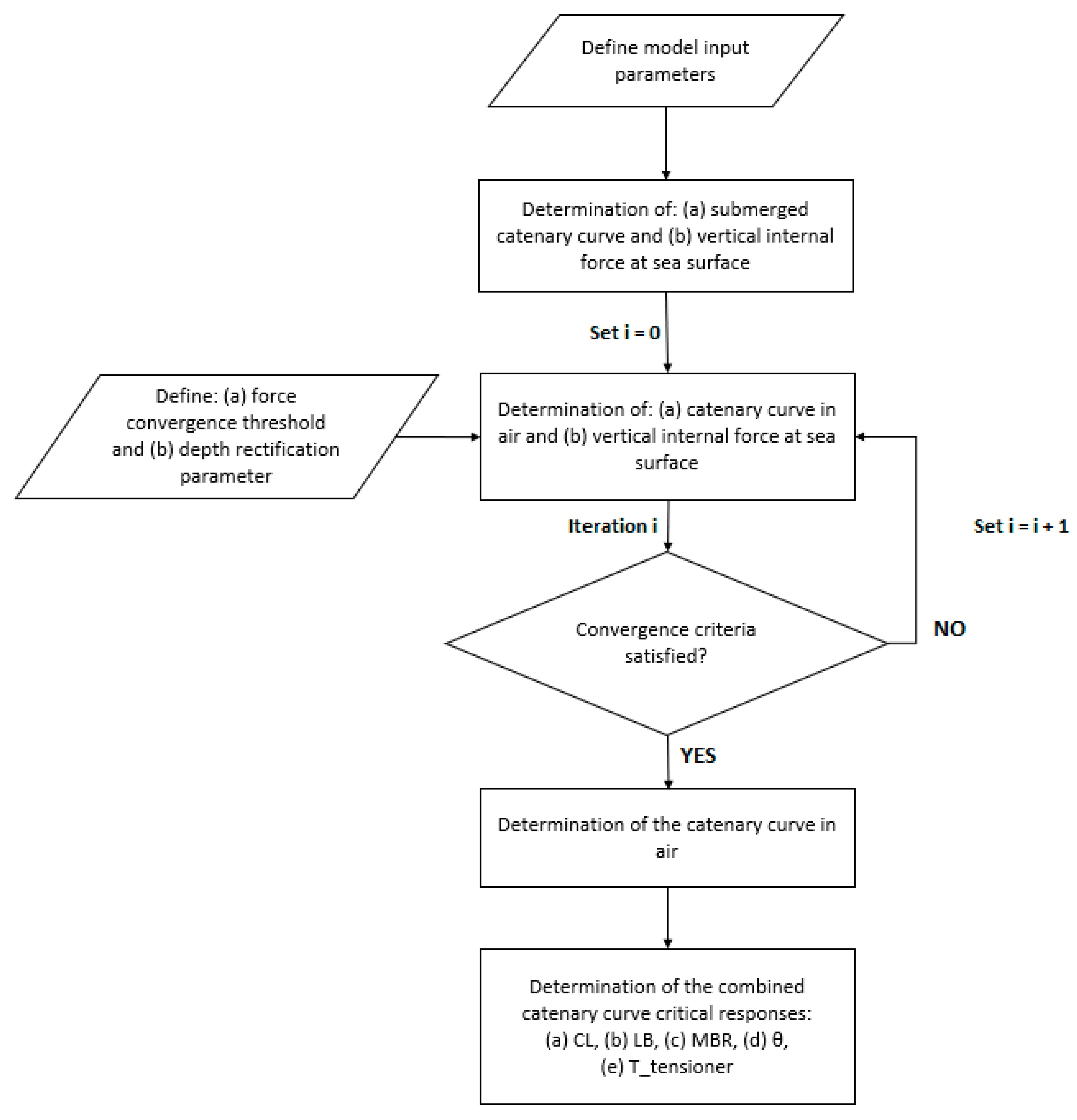
Initially, the submerged catenary curve will be determined using Equation (10). For y = y1 =WD and q = q1, x1 can be calculated assuming a desired bottom tension H.

$$x=\frac{H}{q1}\mathrm{arccosh}\left(\frac{y1\ast q1}{H}+1\right),$$

(10)

For x = x1, the vertical component of the internal force V′ at the dummy node located at the sea surface can be determined using Equation (11).

$$V^{\prime }=\mathrm{H}\ast \sinh \left(\frac{q1\ast x1}{H}\right),$$

(11)

The iterative procedure to define the catenary curve in air, will follow. For the first iteration, we set y = y2 = WD and q = q2, and then x2 is determined using Equation (10) and V″ using Equation (11). The iterative procedure will continue until V″ is almost equal to V′, assuming a difference less than the force convergence threshold as defined by the user. At each iteration, the y is rectified by the depth rectification factor until the convergence has been achieved. At the end of the iterative procedure, the x2 and y2 parameters of the catenary curve in air have been determined.

For y = y2 + c and q = q2, x2′ can be defined using Equation (10). For x = x2′, q = q2 and H_out = H, the vertical force component V_out at the exit point of the overboard chute can be calculated using Equation (12).

$$V_{out}={\mathrm{H}}_{out}\ast \sinh \left(\frac{q2\ast x{2}^{\prime }}{H}\right),$$

(12)

The tangential cable internal force at the overboard chute exit point can be calculated using Equation (13) and the exit angle θ using Equation (14).

$$T_{out}=\sqrt{H_{out}{}^2+V_{out}{}^2},$$

(13)

$$\theta =arctan\left(\frac{V_{out}}{H_{out}}\right),$$

(14)

Therefore, Equation (9b) can be transformed into Equation (15) in order to be integrated into the in-house analysis tool’s numerical formulation.

$$Fr=T_{out}-T_{tensioner}=e^{\left[-sign\left(v\right)\ast \mu \ast \theta \right]}$$

(15)

$$T_{tensioner}=\frac{T_{out}}{e^{\left[-sign\left(v\right)\ast \mu \ast \theta \right]}}$$

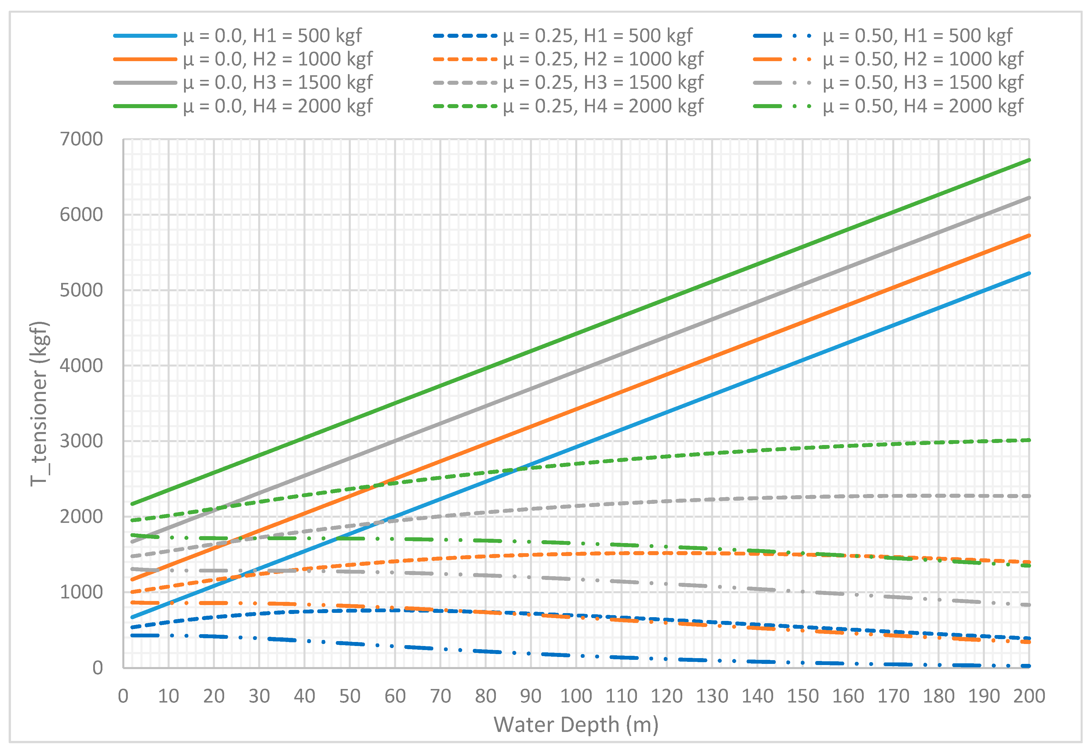
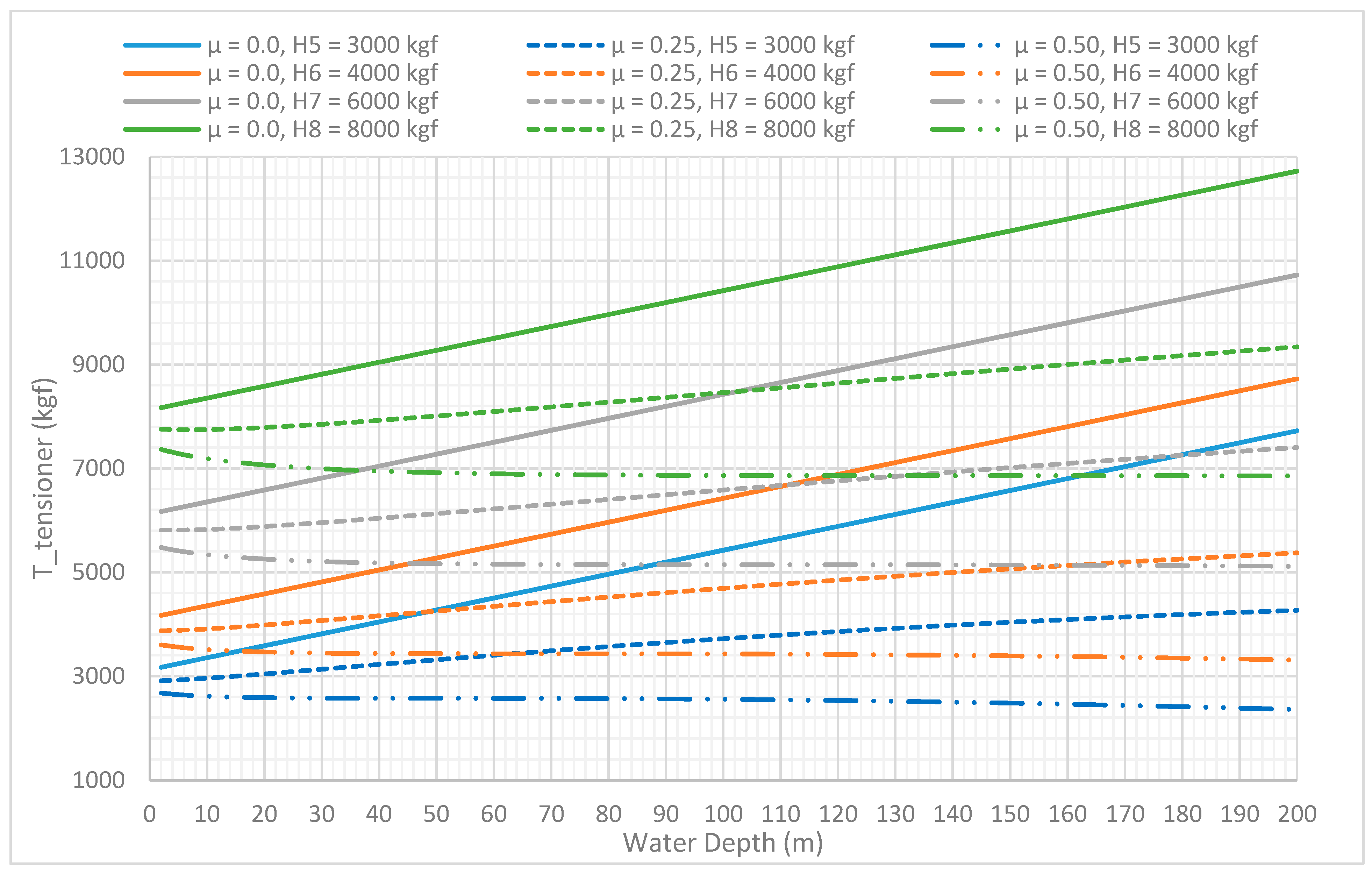
Evaluation of the cable chute friction modelling effects will be conducted analysing cable deployment cases using different friction coefficient values. Initially, three different values of the friction coefficient will be considered (μ = 0.0—μ = 0.25—μ = 0.50) analysing cases at various water depths (between 2 m and 200 m) and different desired bottom tensions (between 500 kgf and 8000 kgf). Figure 19 presents the variance of the cable tension at ship (T_tensioner) assuming various water depths for the bottom tension values of 500/1000/1500/2000 kgf. Similarly, Figure 20 presents the relevant variance of the cable tension ship for the bottom tension values of 3000/4000/6000/8000 kgf.

As illustrated in the above figures, the cable tension at ship (T_tensioner) is dramatically affected by the friction force created between cable and the sliding surface of the overboard chute. It should be noted that in case of no present friction on the overboard chute (cable chute with low friction rollers), the tension machine should be adjusted continuously as the water depth is varying in order to achieve an almost constant bottom tension along the cable route. In case that the friction is present (cable chute with sliding surface), the tension machine adjustment depends on the friction coefficient that has been assumed. It is observed that if the friction coefficient is equal to 0.50, as the water depth is increased and the exit angle (equal to wrap angle) is increased as well, the tension machine adjustment has a gently descending trend. In contradiction, if the friction coefficient is equal to 0.25, the tension machine adjustment has a gently ascending trend as the water depth is increased. Therefore, there is a friction coefficient between the value 0.25 and 0.50 where the friction can be used as a natural tension compensator for a cable laying process without adjusting the tension machine during laying as the water depth is increased or decreased. This observation can be further developed proposing cable chutes with specific friction in order to minimize the tensioner capacities for a cable laying operation. Special attention should be paid that the friction can be used advantageously during a typical laying process, however during a cable recovery operation the friction requires extra force to be exerted by the tensioner in order to retrieve the cable from the seabed. 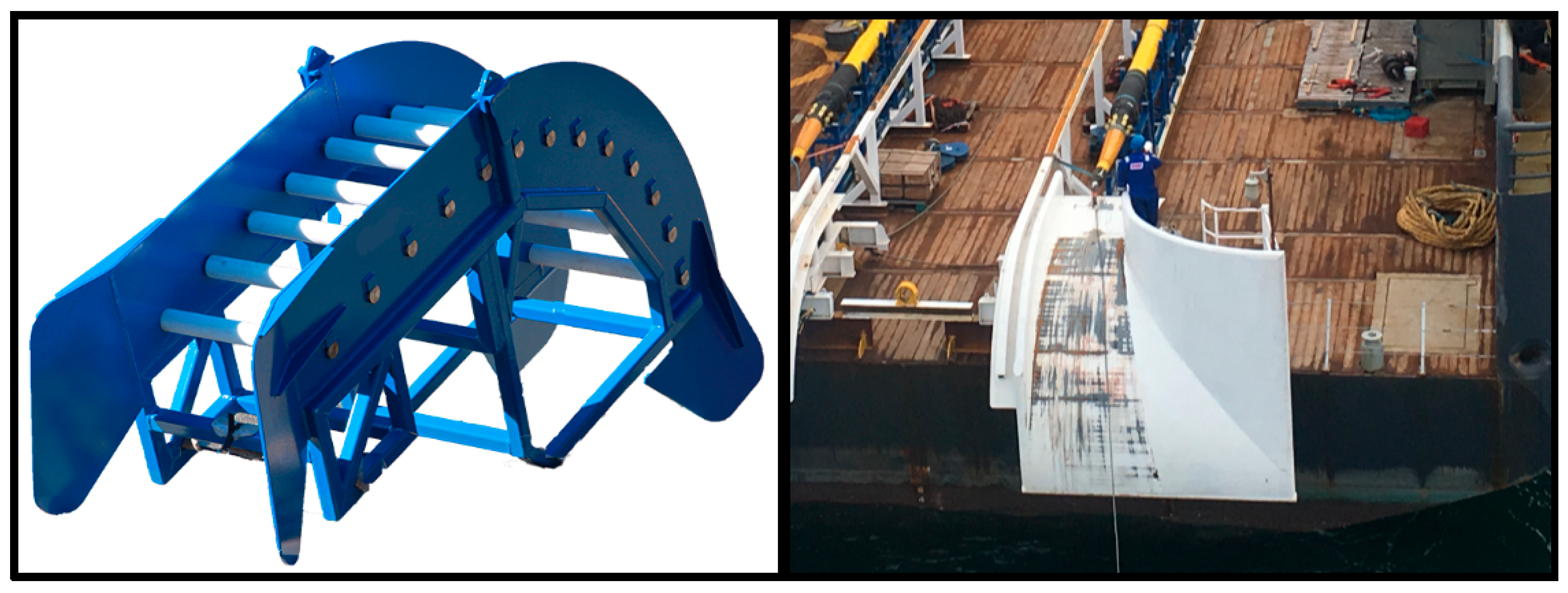Figure 21 presents typical cable chutes from the cable industry, left side with rollers to eliminate the friction and right side with a steel sliding surface where the scratches created by the friction are easily visible.

Nowadays, the cable installers during a cable deployment process use the real time force monitoring capability provided by the load cells of the typical caterpillar or wheel tension machines onboard in order to estimate the cable configuration and the bottom tension on the sea floor. As presented above, the cable tension at ship which is the force value recorded by the tension machine is affected by the actual friction force created by the contact between cable and the overboard chute. Therefore, an error of the friction coefficient estimation by the cable installer can cause to serious misleading results exported by the cable analysis tools that can put in danger the cable integrity. Two case studies will be conducted in order to present the possible analysis error that can be created by assuming a wrong friction coefficient. In the first study, CS1, the cable installer assumes that the friction coefficient at the overboard chute is equal to 0.50 and in order to achieve a desired bottom tension of 3000 kgf at four different water depths 10/50/100/200 m, the tension machine must be adjusted as per the values provided by the analysis tool.

Table 5. Cable critical responses assuming friction coefficient μ = 0.50.

Water Depth (m)	Friction Coefficient μ = 0.5
	T_tensioner kgf	H kgf	LB m	CL m	θ deg	MBR m
10	2613	3000	58.11	60.11	26.5	93.99
50	2574	3000	114.19	129.38	45.39	130.43
100	2555	3000	154.88	193.95	56.41	130.43
200	2359	3000	207.65	307.19	67.14	130.43

presents the critical cable responses for a friction coefficient 0.50.

Table 6. Cable critical responses assuming friction coefficient μ = 0.0.

Water Depth (m)	Friction Coefficient μ = 0.0
	T_tensioner kgf	H kgf	LB m	CL m	θ deg	MBR m
10	2613	2260	50.3	52.59	30.09	74.14
50	2574	1300	72.52	94.15	59.64	56.52
100	2555	130	20.87	108.89	87.04	5.74
200	2359	Compression at TDP, Buckling Failure

and

Table 7. Cable critical responses assuming friction coefficient μ = 0.25.

Water Depth (m)	Friction Coefficient μ = 0.25
	T_tensioner kgf	H kgf	LB m	CL m	θ deg	MBR m
10	2613	2635	54.4	56.53	28.1	84.19
50	2574	2220	97.24	114.57	50.53	96.52
100	2555	1865	118.57	165.6	64.21	81.09
200	2359	1550	139.34	262.17	75.69	67.39

present how the critical responses can be affected in case of having a different friction coefficient (μ = 0.0 and μ = 0.25 respectively) from what initially assumed while maintaining the original tension machine adjustment. As it can be observed, the results prove that the friction can affect drastically the cable configuration and can lead even to a possible cable damage due to buckling or loop formation.

It is obvious that the critical responses of the cable during laying are completely different of what is the cable installer’s understanding due to the wrong estimation of the friction between cable and overboard chute. Special attention should be paid because the cable tension at ship (T_tensioner) is the same for all cases and the cable installer assumes that the cable configuration below the sea surface is exactly what the analysis tool exported. Furthermore, it is observed that the error has an ascending trend as the water depth is increased. Generally, assuming a higher friction coefficient than it is in practice has a result of a lower bottom tension on the seabed and a steeper cable configuration. The wrong estimation of the friction coefficient can lead from an inability to follow a prescribed trajectory on seabed especially along curved routes due to the major error of the layback distance up to a cable failure/damage during the deployment process as presented in Table 6. 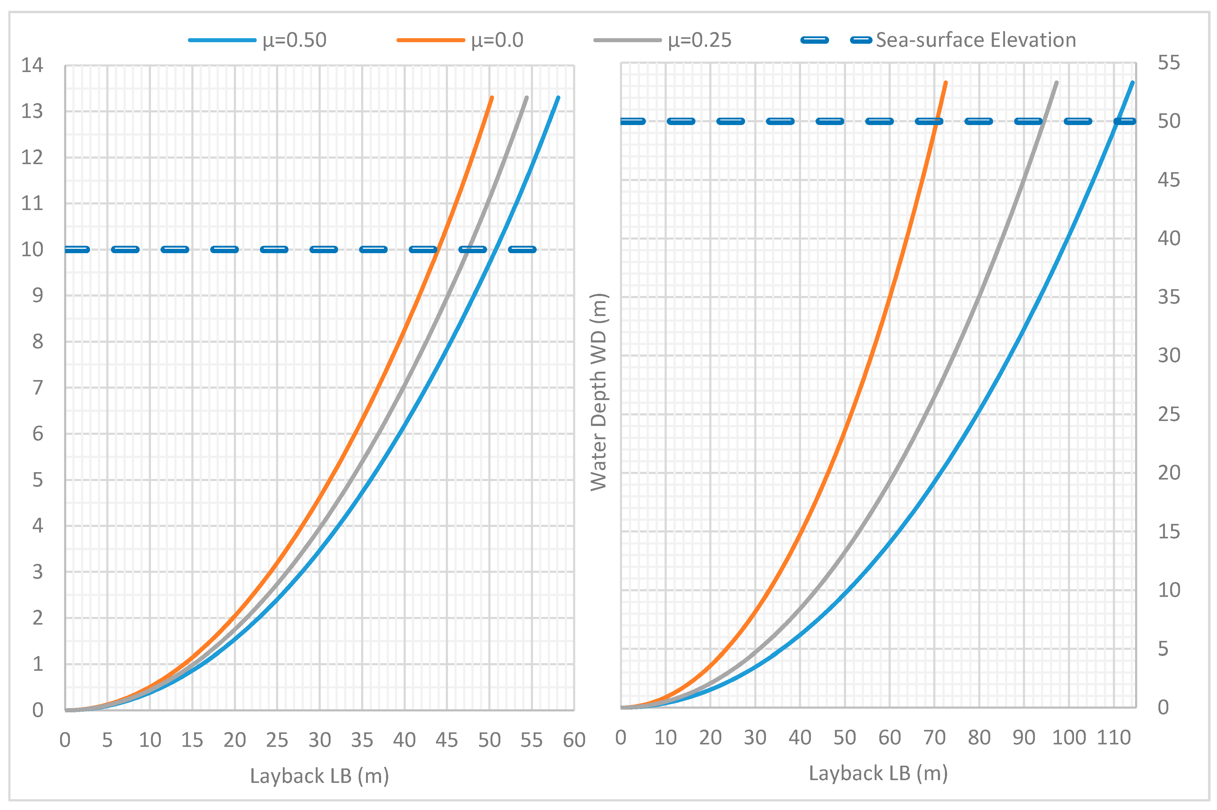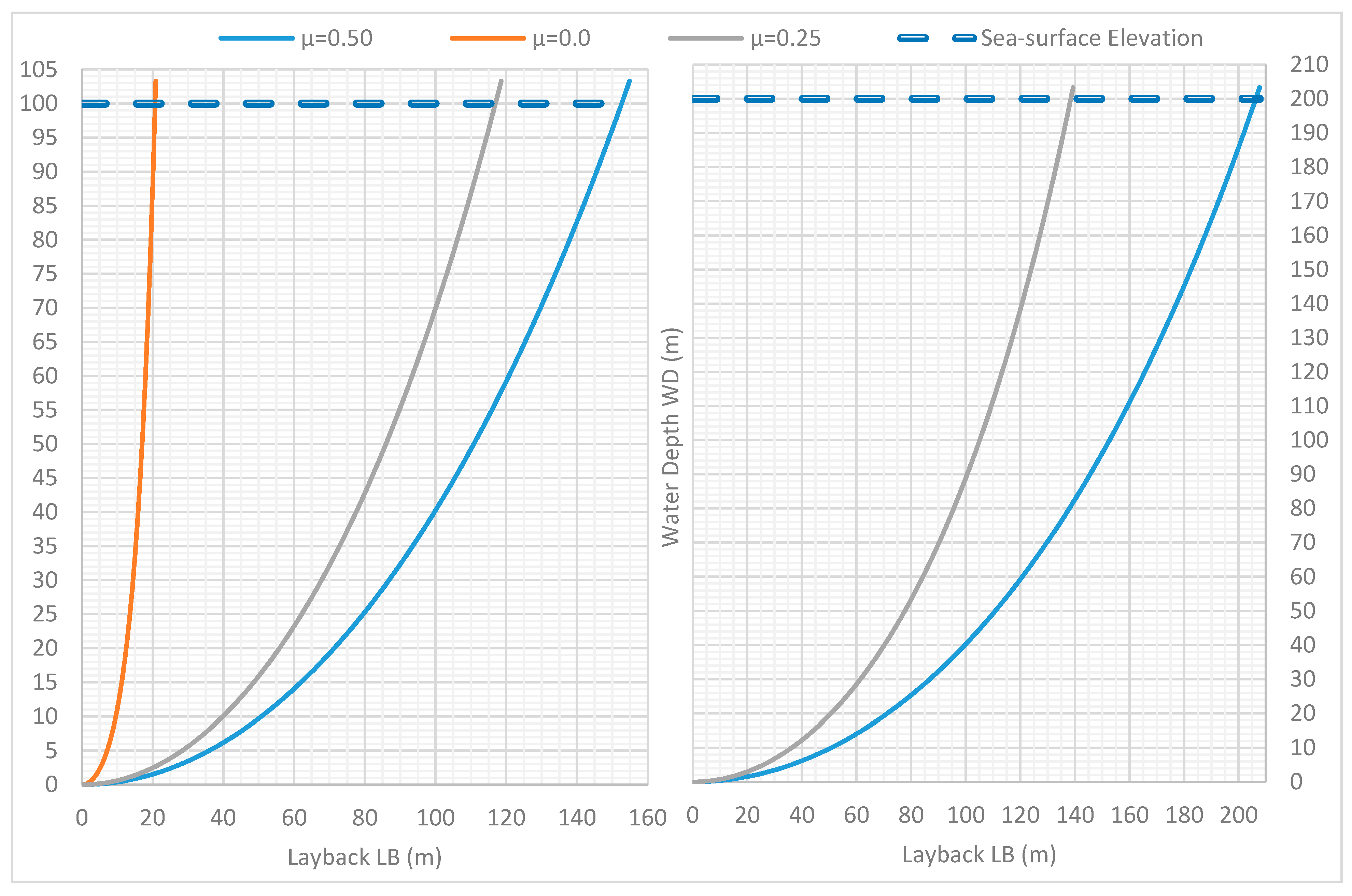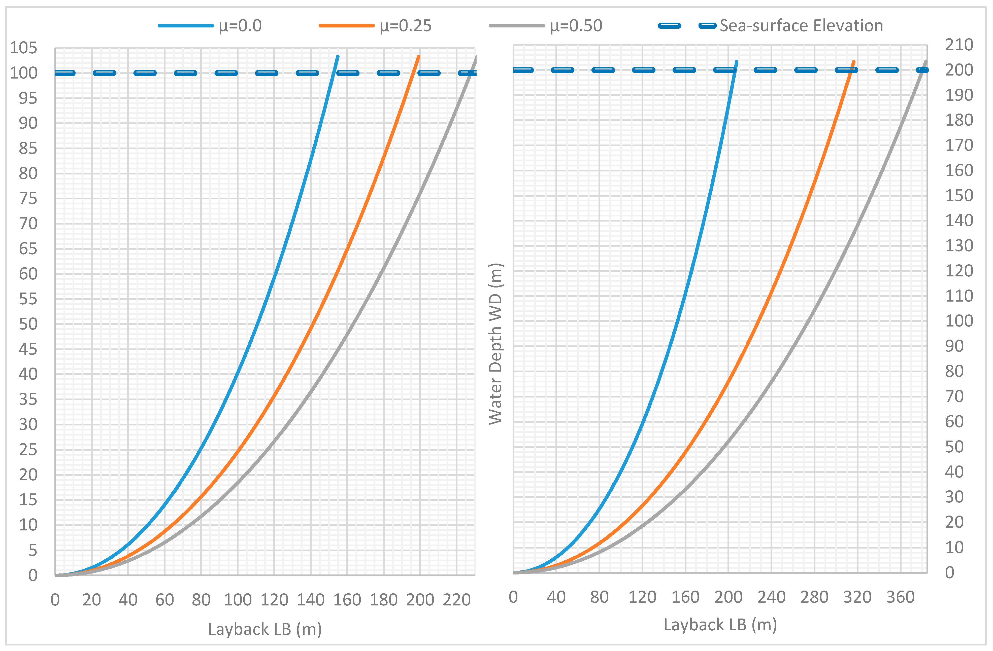Figure 22 and Figure 23 present how the cable configuration can be affected due to the different value of the friction coefficient at various water depths 10/50 m and 100/200 m, respectively. At each figure, the blue line is the cable configuration as per the cable installer’s understanding assuming that the friction coefficient is 0.50. However, grey and orange lines are the real practice due to the actual friction coefficient. It should be noted that in Figure 23, at 200 m water depth, the orange line that represents the case with no friction between cable and overboard chute is not illustrated due to the cable damage caused by the compression force at the TDP.

In the second study, CS2, the cable installer assumes that there is no friction between cable and overboard chute and in order to achieve a desired bottom tension of 3000 kgf at four different water depths 10/50/100/200 m, the tension machine must be adjusted as per the values provided by the analysis tool.

Table 8. Cable critical responses assuming friction coefficient μ = 0.0.

Water Depth (m)	Friction Coefficient μ = 0.0
	T_tensioner kgf	H kgf	LB m	CL m	θ deg	MBR m
10	3353	3000	58.11	60.11	26.5	93.99
50	4273	3000	114.19	129.38	45.39	130.43
100	5423	3000	154.88	193.95	56.41	130.43
200	7723	3000	207.65	307.19	67.14	130.43

presents the critical cable responses for a friction coefficient 0.0.

Table 9. Cable critical responses assuming friction coefficient μ = 0.25.

Water Depth (m)	Friction Coefficient μ = 0.25
	T_tensioner kgf	H kgf	LB m	CL m	θ deg	MBR m
10	3353	3420	62.11	63.99	24.95	105.28
50	4273	4020	133.21	146.5	40.57	174.78
100	5423	4770	199.23	231.33	48.45	207.39
200	7723	6330	316.6	391.33	55.07	275

and

Table 10. Cable critical responses assuming friction coefficient μ = 0.50.

Water Depth (m)	Friction Coefficient μ = 0.50
	T_tensioner kgf	H kgf	LB m	CL m	θ deg	MBR m
10	3353	3820	65.69	67.47	23.71	116.05
50	4273	4980	148.92	160.97	37.2	203.93
100	5423	6320	231.35	259.68	43.7	274.78
200	7723	9000	383.58	447.89	49	391.74

present how the critical responses can be affected in case of having a different friction coefficient (μ = 0.25 and μ = 0.50 respectively) from what initially assumed while maintaining the original tension machine adjustment. As it can be observed, the results prove again that the friction can affect drastically the cable configuration and can lead even to a possible cable damage due to high tensile forces.

It is clear that the critical responses of the cable during laying are completely different of what is the cable installer’s understanding due to the wrong estimation of the friction between cable and overboard chute. Similar to the CS1, it is observed that the error has an ascending trend as the water depth is increased. Generally, assuming a lower friction coefficient than it is in practice has a result of a higher bottom tension on the seabed and a smoother cable configuration. This may increase the minimum bending radius; however, the high tensile forces can damage the more sensitive fiber optic cables. The wrong estimation of the friction coefficient can lead from an inability to follow a prescribed trajectory on seabed especially along curved routes due to the major error of the layback distance up to a cable failure/damage during the deployment process due to the high tensile forces. 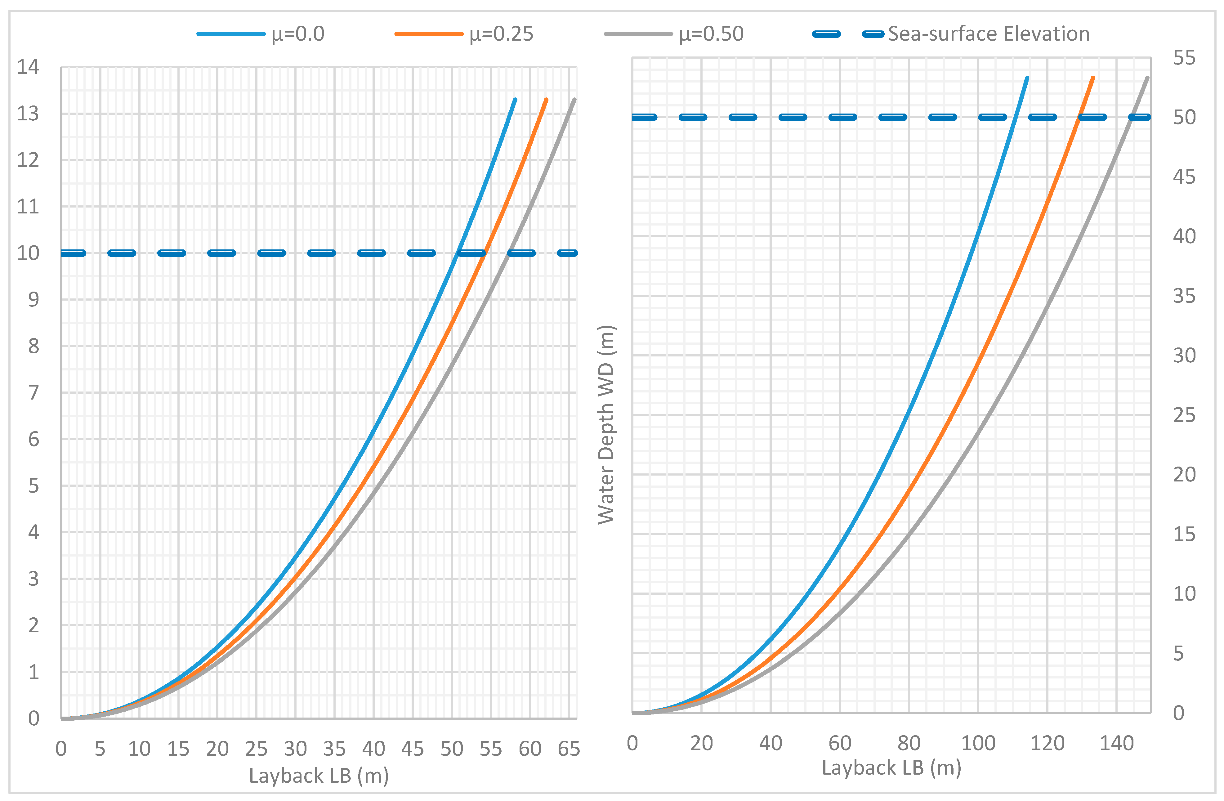Figure 24 and Figure 25 present how the cable configuration can be affected due to the different value of the friction coefficient at various water depths 10/50 m and 100/200 m, respectively. At each figure, the blue line is the cable configuration as per the cable installer’s understanding assuming that there is no friction between cable and overboard chute. However, grey and orange lines are the real practice due to the actual friction which is present.

Both of the examined cases that presented above highlight the importance for the correct estimation of the friction coefficient (μ) required for the accurate calculation of the friction force created by the contact between cable and the overboard chute since this force does affect significantly the critical cable responses. An experimental configuration is proposed for the cable installers in order to verify the actual friction force component which is created on the overboard chute assuming various cable exit angles. Once the friction coefficient has been experimentally defined, the proposed custom-made analysis tool can be utilized in order to predict accurately the cable configuration.

4. Conclusions

The present study focuses on the analysis of various submarine cable deployment cases, highlighting the importance of the water depth and bottom tension combined effects, considering for the first time the “out of water” cable segment. Effect of variations in water depth and bottom tension values in the most crucial installation parameters are examined and presented in form of generic-use installation curves. Moreover, an analytical expression of the critical water depth is provided. The concept of the critical water depth is proposed for the first time in the cable industry to assist cable installers defining the cases in which the “out of water” cable segment can be ignored without denoting the accuracy of the results. Correction factors in relation to the actual WD and H combinations are also proposed improving remarkably the MBR calculation accuracy in case of modelling only the submerged part of cable.

The friction created between cable and overboard chute is numerically defined and incorporated in the custom-made analysis model as a further development of the tool, getting for the first time the attention it deserves. The relevant studies can prove that both modelling and accurate quantification of the friction force should be further investigated since they significantly affect the cable responses. The wrong estimation of the friction coefficient can lead from an inability to follow a prescribed trajectory on seabed especially along curved routes due to the major error of the LB up to a cable failure/damage during the deployment process.

The most important conclusions of this study can be concisely pointed out as follows:

• Layback distance, catenary length and exit angle are not influenced significantly if the “out of water” cable segment is ignored.
• Calculation error for the minimum bending radius is varying between 35–59% at shallow water areas under different bottom tensions between 500 kgf and 8000 kgf.
• Multiplying correction factors are varying between 0.629 and 1.0 and are applied to the original results in which the “out of water” segment has not been modelled.
• Utilizing the proposed correction factors, the initial maximum error of 59% can be minimized even to 1%, increasing the safety standards during the laying activities.
• The modelling and the correct quantification of the actual friction force between cable and overboard chute can provide positive and negative effects during cable laying and recovery activities.
• The overestimation of the actual friction coefficient can cause a cable buckling failure due to an unsatisfactory top tension during a cable deployment in deep water.
• An actual high friction coefficient at the overboard chute can minimize the required capacity of the onboard tensioning machine, eliminating the cost and increasing the availability of the said equipment during laying activities. The opposite is valid during the cable recovery activities.
• A specific friction coefficient between the values of 0.25 and 0.50 can be advantageously utilized as a natural compensation of the cable self-weight.
• The modelling of the “out of water” cable segment is critical in shallow water and the modelling of the friction force between cable and overboard chute is critical in deep water. The proposed analysis tool can handle both of the cases providing reliable results.

The proposed custom-made analysis tool that is used with this paper is planned to be further extended including nonlinear effects. In regard to the actual friction forces introduced by the contact between cable and overboard chute, laboratory experiments are planned to be performed assuming various sliding surfaces of chutes, varying exit angles and ship top tensions providing a safe estimation of the actual friction coefficient for each cable chute category.