Effect of Skeg on the Wave Drift Force and Directional Stability of a Barge Using Computational Fluid Dynamics

1
Division of Navigation Science, Korea Maritime and Ocean University, Busan 49112, Korea
2
Division of Marine Industry Transportation Science and Technology, Kunsan National University, Jeonbuk 54150, Korea
*
Author to whom correspondence should be addressed.
J. Mar. Sci. Eng. 2020, 8(11), 844; https://doi.org/10.3390/jmse8110844
Submission received: 28 September 2020
/
Revised: 17 October 2020
/
Accepted: 24 October 2020
/
Published: 27 October 2020
(This article belongs to the Section Ocean Engineering)
Abstract
:To accurately estimate the navigation safety of a barge in still water and waves, computational fluid dynamics (CFD) was used to calculate the hydrodynamic force on the barge and simulate the flow field to comprehensively study the effect of skeg for wave drift force and directional stability of the barge. With respect to the wave drift force, the steady surge force and steady sway force are found to decrease due to the skeg effect in both short and long wavelength regions. The overall steady yaw moment tends to be reduced by the skeg. As the drift angle increased, the sway force and yaw moment also increased. The changing trend in the sway force varied with the angular velocity, depending on the installation of the skeg, and it was noted that the yaw moment value significantly increased because of the skeg. Owing to the effect of the skeg installed on the barge, the yaw damping lever became larger, while the sway damping lever became smaller regardless of waves. It was confirmed that the directional stability was improved both in still water and head waves.
1. Introduction
In the stern towing method where a tug pulls a barge from the stern side, the directional stability of the barge is one of the most important factors in the operation of the tug-barge system. While navigating tug and barge, the yaw motion of the barge should be reduced to ensure a safe towing operation because it limits the steering performance of the tug. Therefore, it is necessary to accurately estimate and evaluate the directional stability of the barge to ensure its safe navigation. Studies have been conducted to prove that installing a skeg is an effective method to improve the stability of the barge in still water. Inoue et al. [1] conducted various experiments on different types of skegs; they reported that the directional stability of the barge is greatly affected by the type of skeg and the installation conditions. Experiments showed that directional stability could be improved by installing the knuckle-type skeg to a bare-hull barge, having a yaw amplitude that was 10 times the vessel width [2]. The study on the directional stability of the barge in still water was conducted by experimental [3] and numerical methods [4], and the characteristics of the maneuvering performance of the barge were analyzed. Previous studies have focused on the optimal arrangement and shapes of skeg for a specific barge in still water.
To estimate the maneuvering performance of the vessel, it is necessary to determine the derivatives of the hydrodynamic force that includes the angular velocity and drift angle as variables. Most of the existing studies have been able to calculate this using the empirical equations of the vessel or obtaining the coefficients through experiments. Numerical computation based on the potential theory has limitations when it comes to precisely calculating the effects of interference and viscous effects between the attachment and hull, which affect maneuvering performance. Furthermore, in case the ship’s speed is not high enough to affect the wave-breaking phenomenon, or because of the efficiency of numerical calculation, the ship’s maneuverability is evaluated without taking into account the influence of free surface [5,6]. However, an actual barge is mostly operated in waves on the sea. The sway force and yaw moment in waves are different from those in still water, and the variation is significant enough to affect the maneuvering performance of the barge. Therefore, it is necessary to estimate accurately the variation in the sway force and yaw moment because of the waves.
Studies on the maneuvering performance of the vessel in waves have been conducted experimentally and theoretically. Hirano et al. [7], Ueno et al. [8], and Yasukawa [9,10] conducted an experimental analysis on a free-running model test for the turning circle and zigzag test. Recently, a free-running test was performed to analyze the effects of wave lengths, heights, and directions on the ship turning trajectories [11]. Tello Ruiz et al. [12] conducted a study to investigate the effect of waves on the ship’s maneuverability in a finite water depth mainly experimentally and to some extent numerically.
Skejic and Faltinsen [13] analyzed ship maneuvering in waves using a unified seakeeping and maneuvering two-time scale model based on the strip theory. Seo and Kim [14] solved the ship maneuvering problem in waves using the time-domain ship motion program based on the Rankine panel method. Zhang et al. [15] calculated the maneuvering motion using maneuvering modeling group (MMG) model and solved the seakeeping problem based on the time domain Rankine panel method. The mean second-order wave loads were included in the MMG model as the wave drift forces. Chillcce and el Moctar [16] presented a numerical method for maneuvering in waves based on nonlinear equations of motion derived with respect to an inertial coordinate system. The still water maneuvering forces were calculated based on hydrodynamic coefficients obtained by RANS planar motion mechanism (PMM) tests, while wave induced forces were calculated using the Rankine boundary element method.
The ships used for the maneuverability evaluation in the waves mentioned above were self-propulsive ones, and most of the numerical calculations were based on potential theory. Few studies have been conducted on towed barge, of which directional stability is an essential requirement in waves. Nonlinear factors must be considered to estimate the sway force and yaw moment acting on a barge when a skeg is attached to the stern side of the barge, or when there is the influence of external forces such as waves. The computational fluid dynamics (CFD) technique can precisely estimate the hydrodynamic force on a vessel in waves containing nonlinear and viscous effects, and it can be used very effectively to evaluate maneuvering performance by analyzing the behavior of the vessel and obtaining the related maneuvering derivatives.
In this study, numerical simulations were performed using CFD to calculate the hydrodynamic forces acting on the barge in still water and head waves for its safe navigation in sea areas. Firstly, the steady wave drift force, which was a nonlinear second order force, was analyzed in consideration of the skeg effect. Next, the static drift motion test and pure yaw motion test were performed to obtain the maneuvering hydrodynamic derivatives. Based on these results, the directional stability of the barge in still water and waves considering the skeg effect were evaluated.
2. Numerical Calculation
2.1. Computational Method
STAR-CCM +, a commercial CFD program based on the finite volume method, was used in this study to perform the numerical simulation. The continuity and momentum equations for incompressible flow analysis are as follows:
where represents the mean viscous stress tensor components:
where is the density, denotes the averaged Cartesian components of the velocity vector, denotes the Reynolds stresses, and is the dynamic viscosity.
Temporal discretization of the unsteady term used a first-order temporal scheme, and a second-order scheme was applied to discretize convection terms. The SIMPLE method was used in the velocity-pressure coupling. In the turbulence model, the realizable k-ε model was used and all y+ wall treatment was applied. The k-ε model is used extensively in industrial applications and has advantages in terms of the cost of CPU computation time [17]. For the stability and efficiency of the numerical computation, Sung and Park [18] utilized the realizable k-ε model to conduct a dynamic test on a vessel.
In implicit unsteady simulations, the time step is determined by the flow properties rather than the Courant number [17]. At least 100 time steps per encounter period were used for the simulation in waves as recommended by ITTC [19]. A minimum cell size of 0.0125% of wavelength and 0.0625% of wave height were used in the horizontal and vertical directions, respectively.
A free surface was solved by applying the volume of fluid (VOF) method. The dynamic fluid body interaction (DFBI) function was used to simulate the hull motion [20], with the barge free in heave and pitch.
The fifth-order Stokes wave was selected for the numerical simulation. A regular wave with a wave amplitude in the head direction was analyzed, and the directional stability characteristics were analyzed at wavelengths of 0.5L, 1.0L, and 1.5L (where L denotes the length between perpendiculars). These characteristics were then compared to the characteristics in still water. To confirm the effect of the skeg on the directional stability, numerical computations were performed when the skeg was installed and when the skeg was not installed (bare hull).
2.2. Computational Condition
A 91.5 m barge, which was the size of an actual vessel, was used as a subject vessel when conducting the numerical simulations to analyze the characteristics of hydrodynamic forces acting on the barge in still water and waves. The barge used in the numerical calculation is a round-type model frequently accessed in practice. Table 1 shows the main specifications of the barge, and the basic shapes of the barge are shown in Figure 1. The speed of the barge was set to 7 knots (Froude number ), and the numerical computations were conducted in still water and waves at Reynolds number .
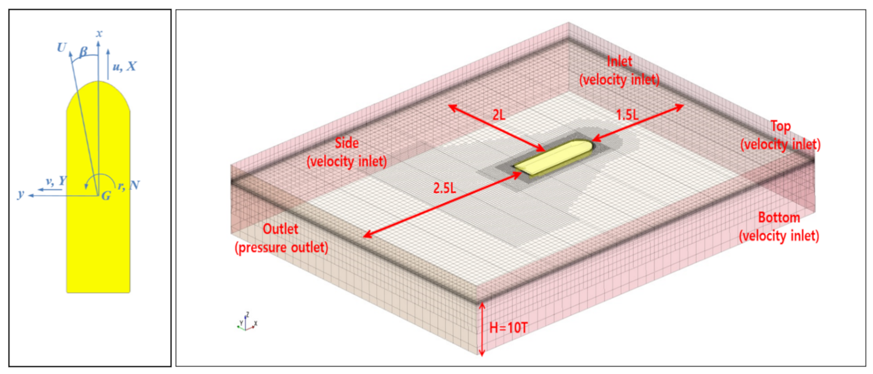
Figure 2 shows the computational domain and coordinate system that was used in this study. It is a Cartesian coordinate system in which the forward direction is the +x-axis, the port direction of the barge is the +y-axis, and the opposite direction of gravity is the +z-axis. , and are the surge force, sway force, and yaw moment, respectively. , , and denote the surge, sway, and yaw velocities, respectively. The numerical simulation was conducted by selecting a computational domain 1.5L, 2.5L, 2.0L, 3.0T, and 10.0T away from the fore perpendicular of the barge, aft perpendicular of the barge, center line to the transverse direction, water surface to the vertical direction, and water surface to the seabed, respectively. The inlet, top, bottom, and side boundaries were selected as velocity inlets. The hull surface was selected as a no-slip boundary condition. Numerical computation was performed using the VOF wave damping functionality of the software with a damping length of 1.0L to avoid wave reflection into the domain.
The space and hull surface grids were created using the trimmed mesh and prism layer, respectively. To implement the flow more precisely in the head, stern, free surface, and divergent regions, the grid size was created to be denser than the base size, using volumetric control. The number of grids used in the numerical simulation was about 1.5 million, and the mean y+ values for at was 181 and 208 at . y+ is the dimensionless wall distance, is the wavelength, is the drift angle, and denotes the nondimensionalized angular velocity by (). Drift angle is the difference between heading and actual course. The detailed grid convergence uncertainty is described in Section 3.1.
In this study, the drift motion test, which is a static test, and the pure yaw motion test, which is a dynamic test, were simulated based on the planar motion mechanism (PMM) to obtain the derivative value of the hydrodynamic force for evaluating directional stability. Velocity-dependent derivatives of the maneuvering hydrodynamic force, and , were calculated from the drift motion test, and rotary derivatives and were calculated from the pure yaw motion test. The drift angle was set to 5°, 10°, and 15°. The direction of the water flow into the barge was set to the port side of the barge. The nondimensionalized angular velocity was set to 0.1, 0.3, and 0.5. In the pure yaw motion test, the sway force (Y) and yaw moment (N) at the position where the yaw angle is at the minimum, i.e., the lateral displacement is at its maximum, are computed. The PMM test procedure and analysis method were performed by referring to the study by Kim et al. [21]. Table 2 shows the test conditions for PMM simulation.
3. Results and Discussion
3.1. Mesh Sensitivity Analysis
This study used the grid convergence index (GCI) method based on the Richardson extrapolation to estimate the grid convergence uncertainty of the numerical simulations. Park et al. [22], Tezdogan et al. [17], and Demirel et al. [23] have applied the GCI method to evaluate numerical uncertainty. The verification process using the GCI method was followed according to the approach described by Celik et al. [24].
The numerical convergence ratio is calculated as follows:
Here, it is obtained by and , each of which represents the difference in the solution value between medium-fine and coarse-medium, respectively. , , or each represent the solution calculated for the fine, medium, or coarse mesh. The convergence ratio calculated as described is classified as follows:
(i) monotonic convergence (), (ii) oscillatory convergence (), (iii) oscillatory divergence (), and (iv) monotonic divergence (1).
The apparent order of the method can be obtained as follows:
where is the grid refinement factor , i.e., used in this study.
The extrapolated values are calculated as shown in Equation (6):
In addition, the approximate relative error and extrapolated relative error are obtained by the following equations, respectively:
Last, the medium-grid convergence index is calculated as follows:
The number of meshes for the grid convergence study is shown in Table 3 when the skeg was not installed. The sway force (Y) and yaw moment (N) were calculated using the number of coarse, medium, and fine grids, and the results are shown in Table 4. As shown in the calculation results, the numerical uncertainty for the medium mesh using the GCI method were estimated to be 3.12% and 9.37%, respectively. According to the results of the grid convergence uncertainty study, it was concluded that efficient numerical simulation is possible using the medium mesh. Therefore, the medium mesh was selected as the base size in this study.
3.2. Analysis of Steady Wave Drift Force
Table 5 shows the linear surge force , sway force , and yaw moment of the barge with and without skeg in still water at the drift angle of 15°. , and became dimensionless by the barge speed (), barge length (), and draft () as shown below.
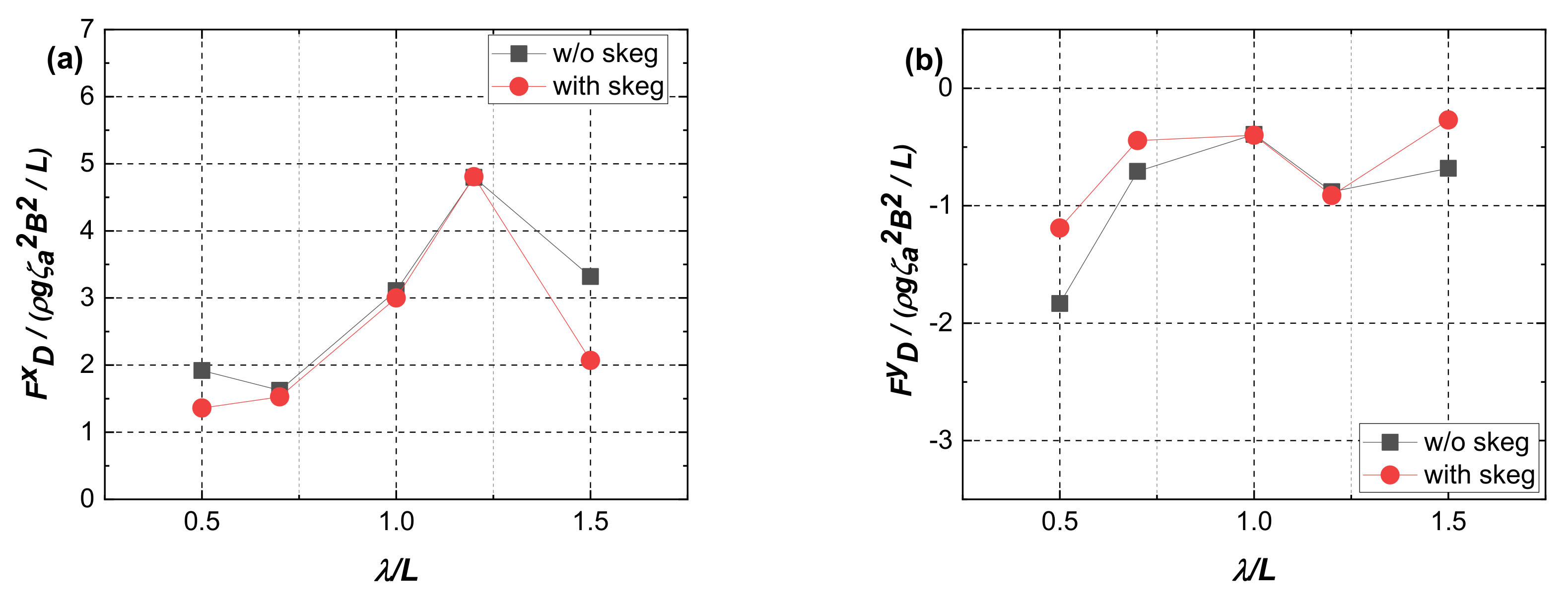
As indicated in Table 5, and values increase due to the installation of an addition such as skeg, and value decreases because of the skeg effect.
However, the steady wave drift force, which is the second order force in waves, shows a different tendency. Figure 3 shows calculation results for cases with and without skeg under conditions with the drift angle of 15°, wave height 1 m, and and in head seas to compare the steady wave drift force. The steady wave drift force is obtained by subtracting the results in still water from the results in waves.
The steady surge force also means added resistance caused by waves. This wave drift force shows the largest value around , and this distribution shows a similar trend as published in other research results [25,26]. In a short wavelength of and a long wavelength of , the steady surge force is found to decrease due to the skeg effect.
The steady sway force shows the largest value at a short wavelength of regardless of the installation of skeg. This seems to be due to the reflected wave effect in short waves as discussed in other studies [25,27]. It can be seen that skeg effect plays the role of reducing the steady sway force in both short and long wavelength areas in the same manner as . It can be presumed that skeg is effective in suppressing drift motions on longitudinal and lateral directions. The changes in hydrodynamic force by skeg are very small at and .
The overall steady yaw moment tends to be reduced by the skeg. The highest reduction amount occurs at , and the skeg rather increases at a short wavelength of . It is shown that the skeg is effective in reducing not only yaw moment , which is the first order force, but also the steady yaw moment value, which is a nonlinear fluid force. It is assumed that this effect reduces sway damping lever to improve directional stability of the barge.
3.3. Static Drift Simulation
In this section, numerical simulation using CFD was carried out to achieve the maneuvering derivatives of the barge in drift motion, and the results are as follows:
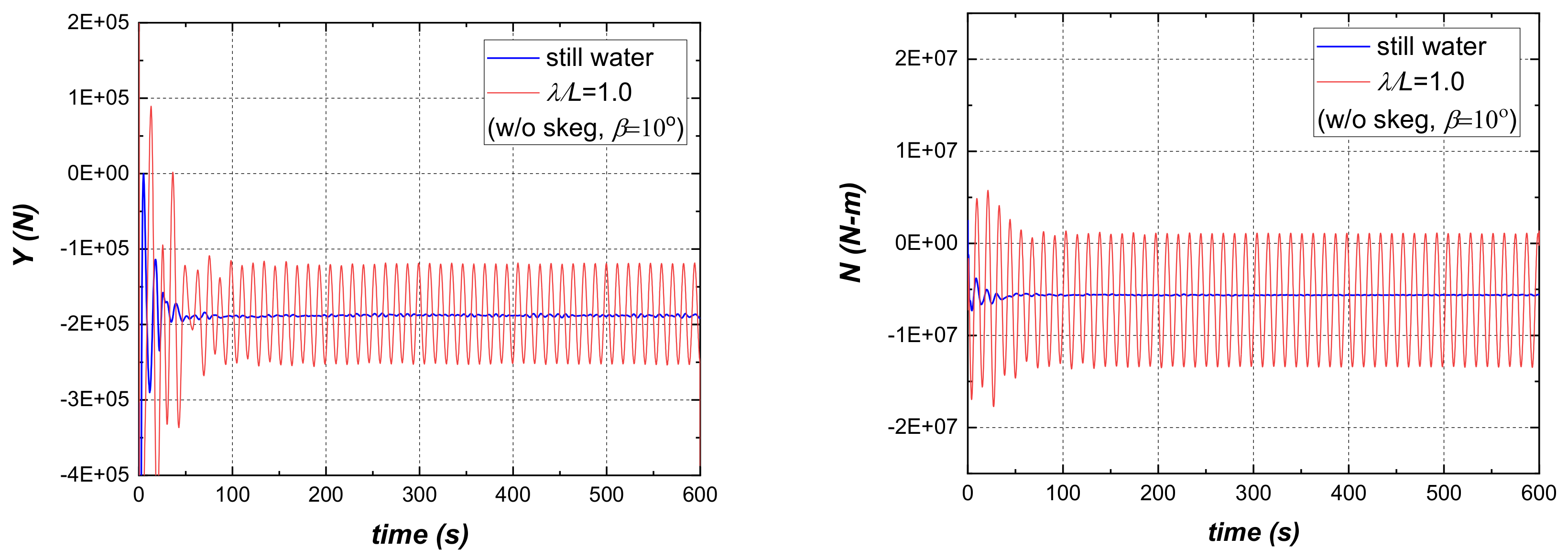
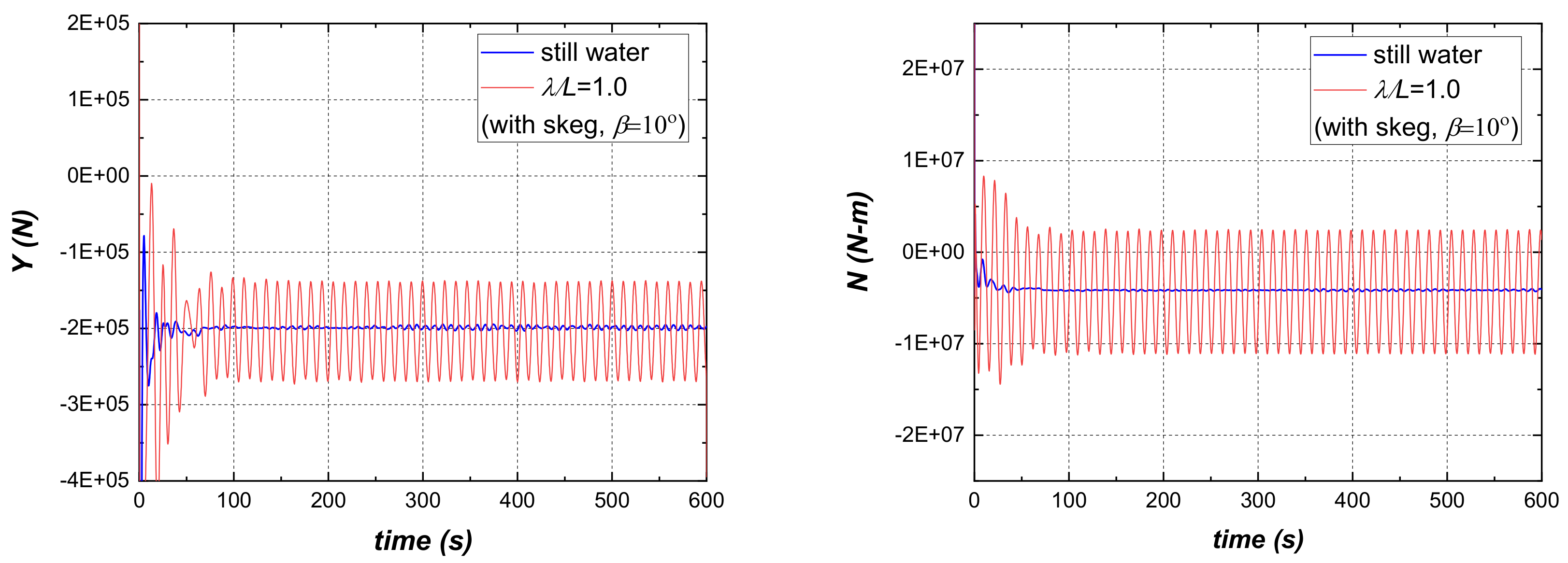
Figure 4 and Figure 5 show the time history for the sway force and yaw moment acting on the barge in still water and waves (). It can be seen that the sway force value is slightly increased by the skeg, and the yaw moment value is decreased. Ten times of the encounter wave period was used to average the sway force and yaw moment.
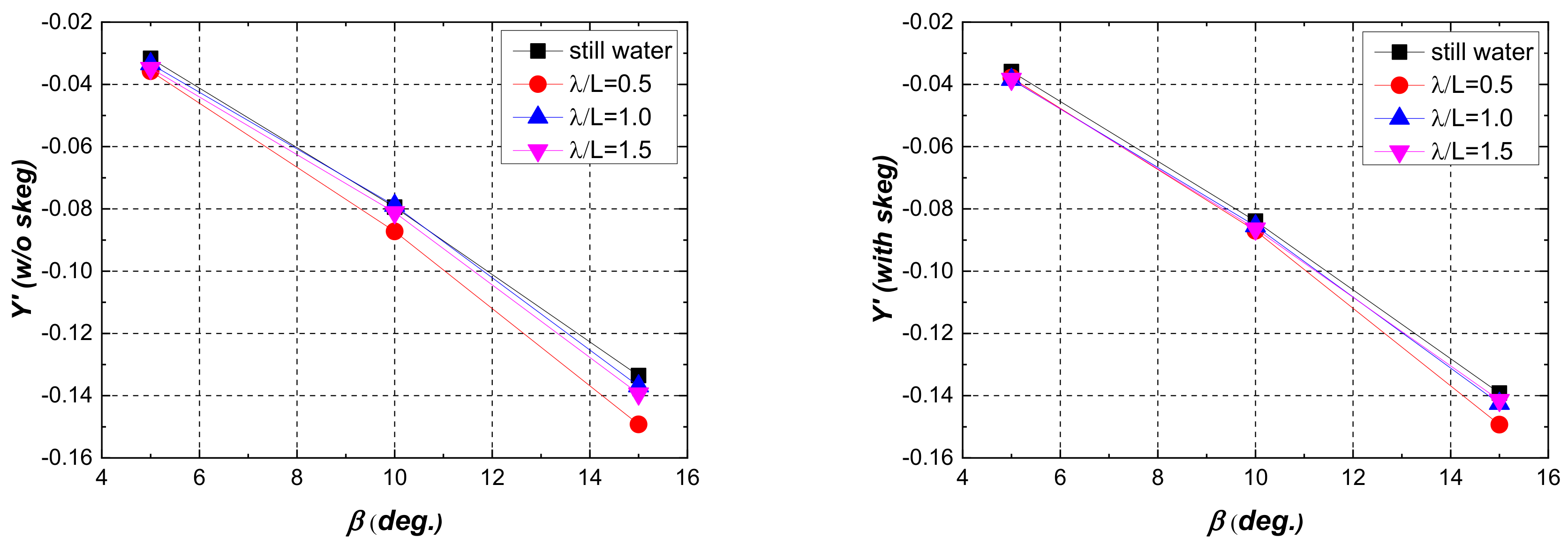
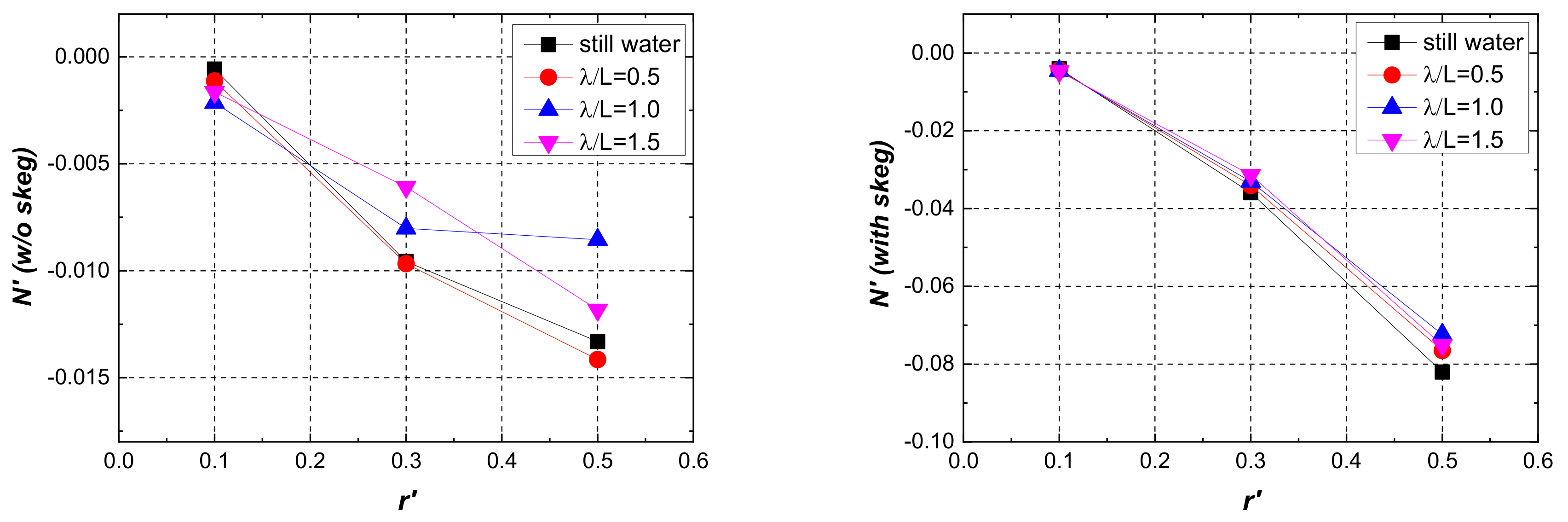
The nondimensionalized sway force () and yaw moment () at each drift angle are shown in Figure 6 and Figure 7. As shown in the figure, as the drift angle increases, the negative value of the sway force and yaw moment increases as well. The greatest sway force occurs in the short wavelength, and the smallest occurs in still water, regardless of the installation of skeg. Although the sway force does not change significantly with the installation of the skeg, the yaw moment shows a relatively large change because of the installation of the skeg. In other words, it was found that the negative value of the yaw moment became smaller with the installation of the skeg.
A transverse velocity component is calculated as follows:
where is the ship’s velocity and is the drift angle. Based on the sway velocity , hydrodynamic derivatives and are produced.
It can be seen that is not much affected by the skeg, and is smaller. It is assumed that the sway damping lever () value is decreased, which can contribute to improving the stability of the barge.
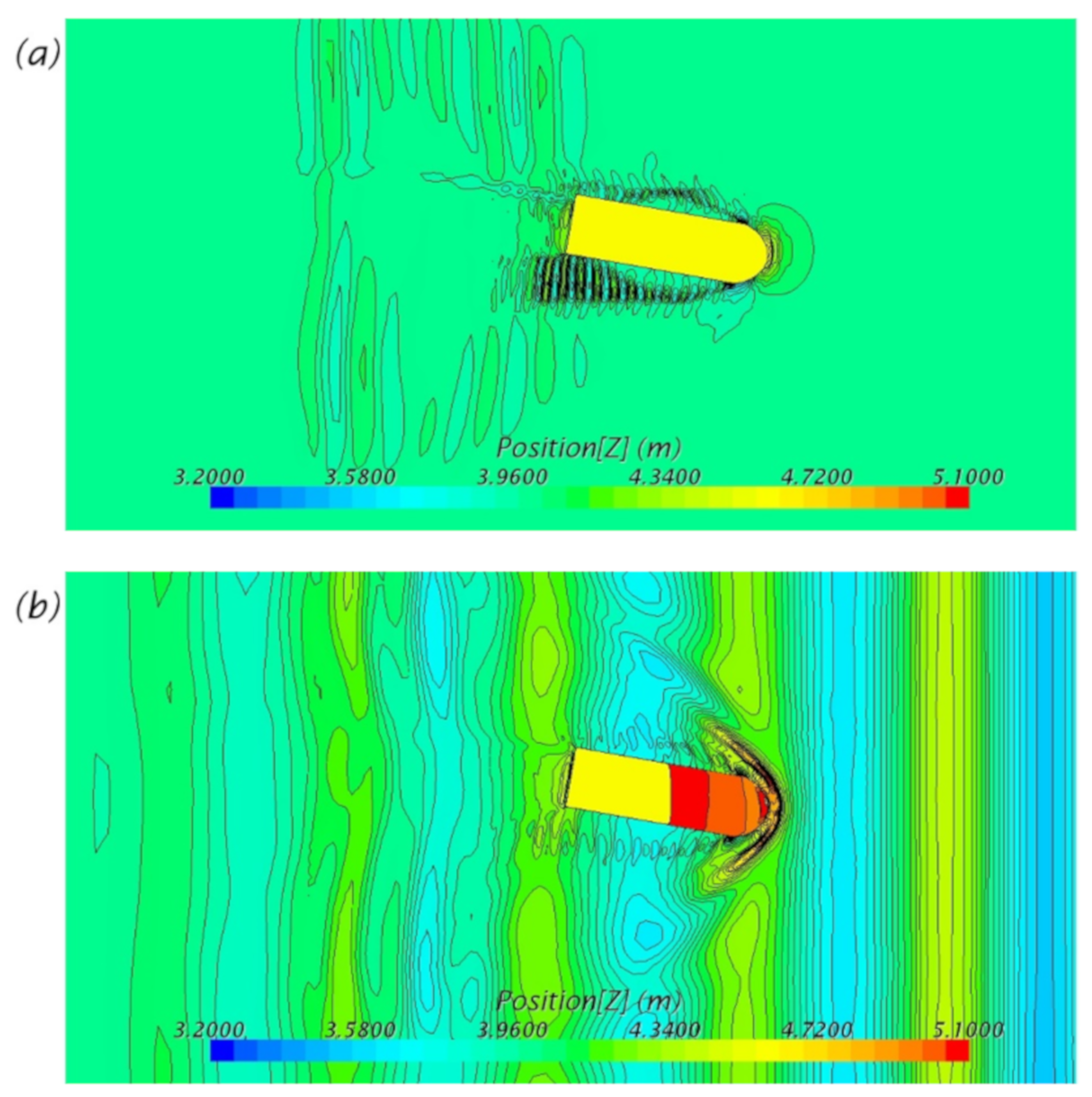
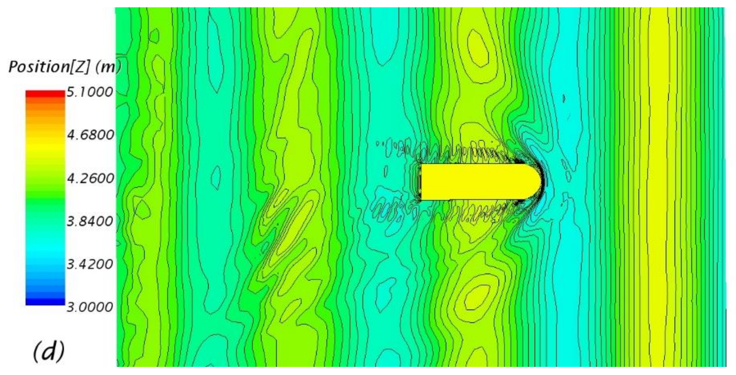
Figure 8 shows wave patterns around a barge without a skeg in still water and in waves with a wavelength of . It can be seen that unbalanced flow fields are generated on the port and starboard sides with a drift angle of 10°.
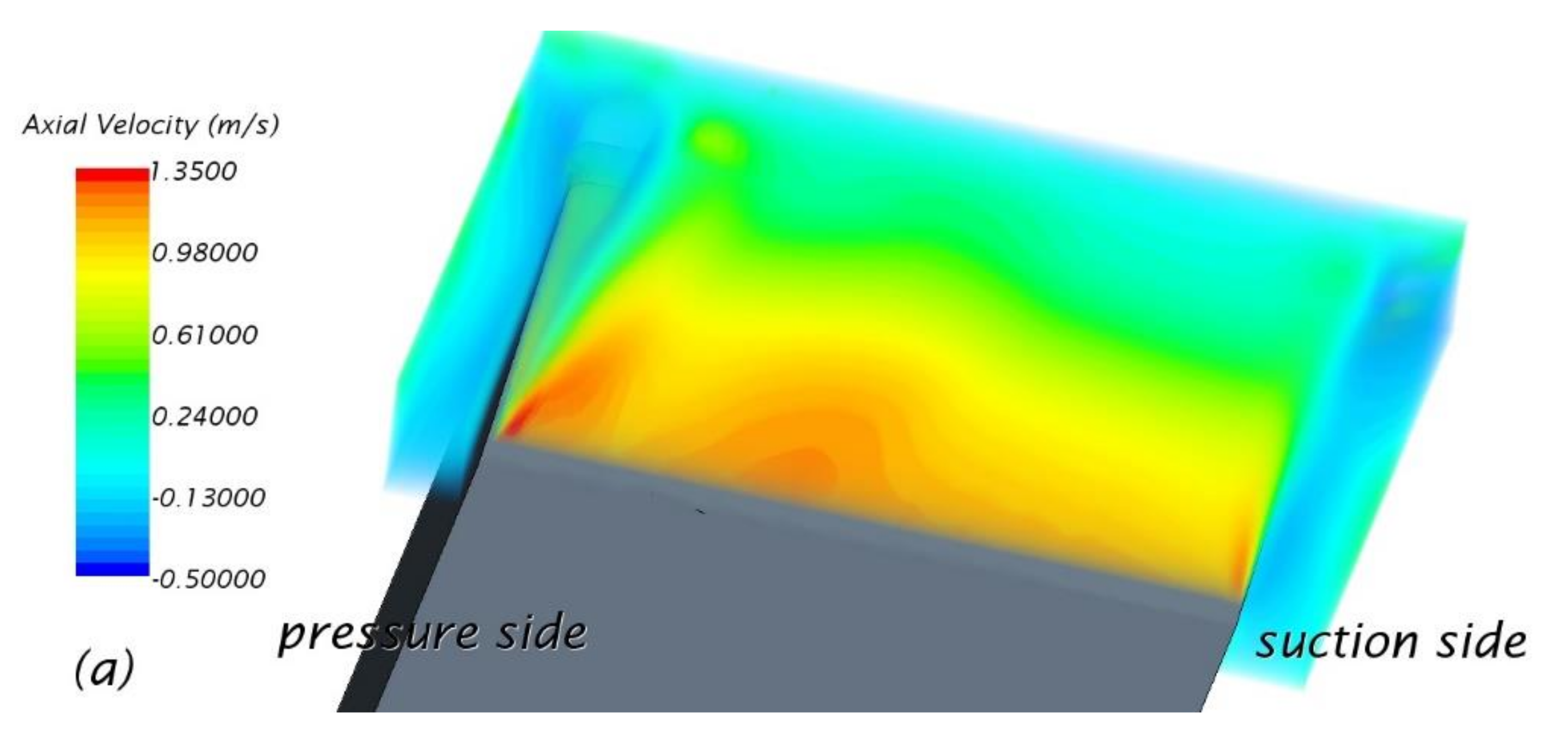
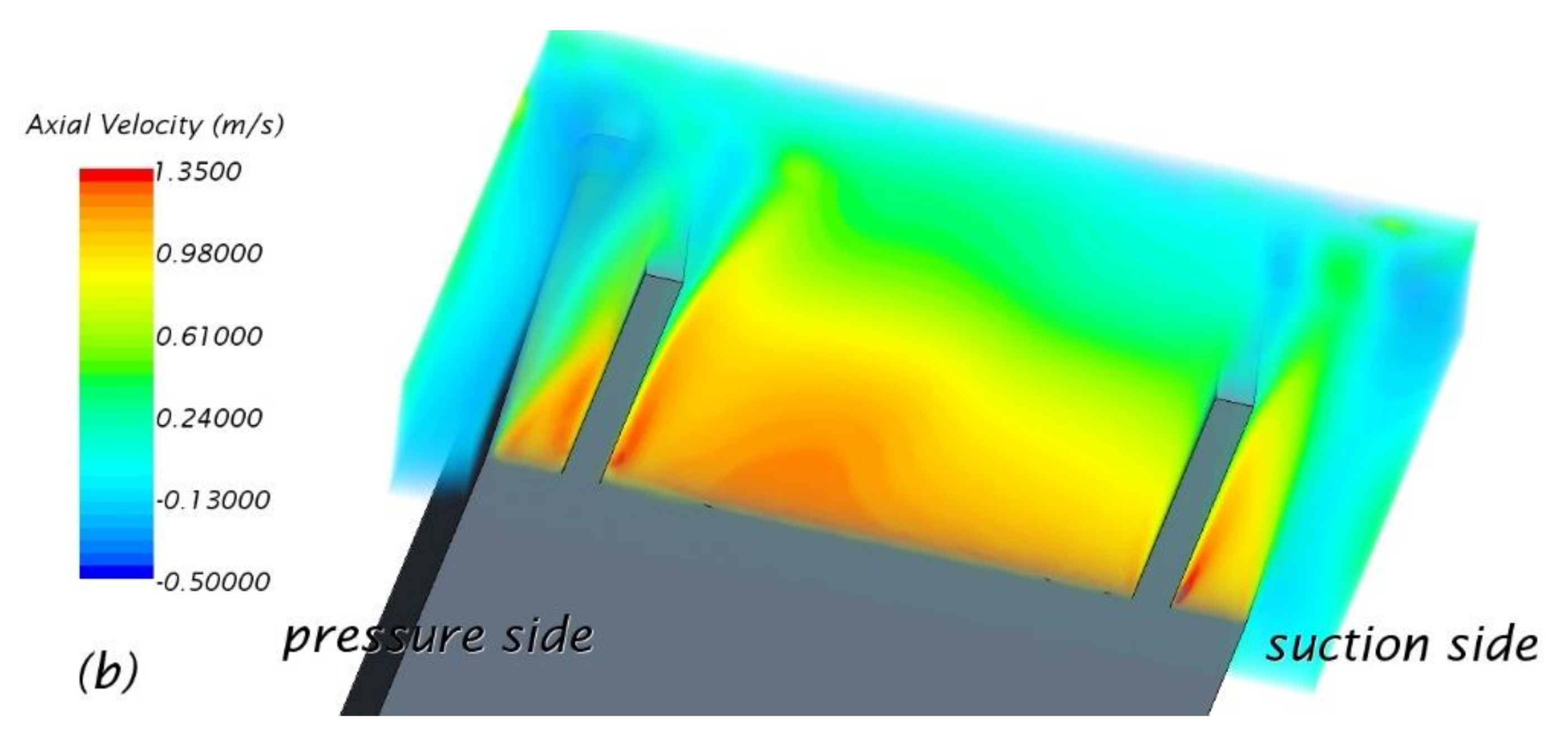
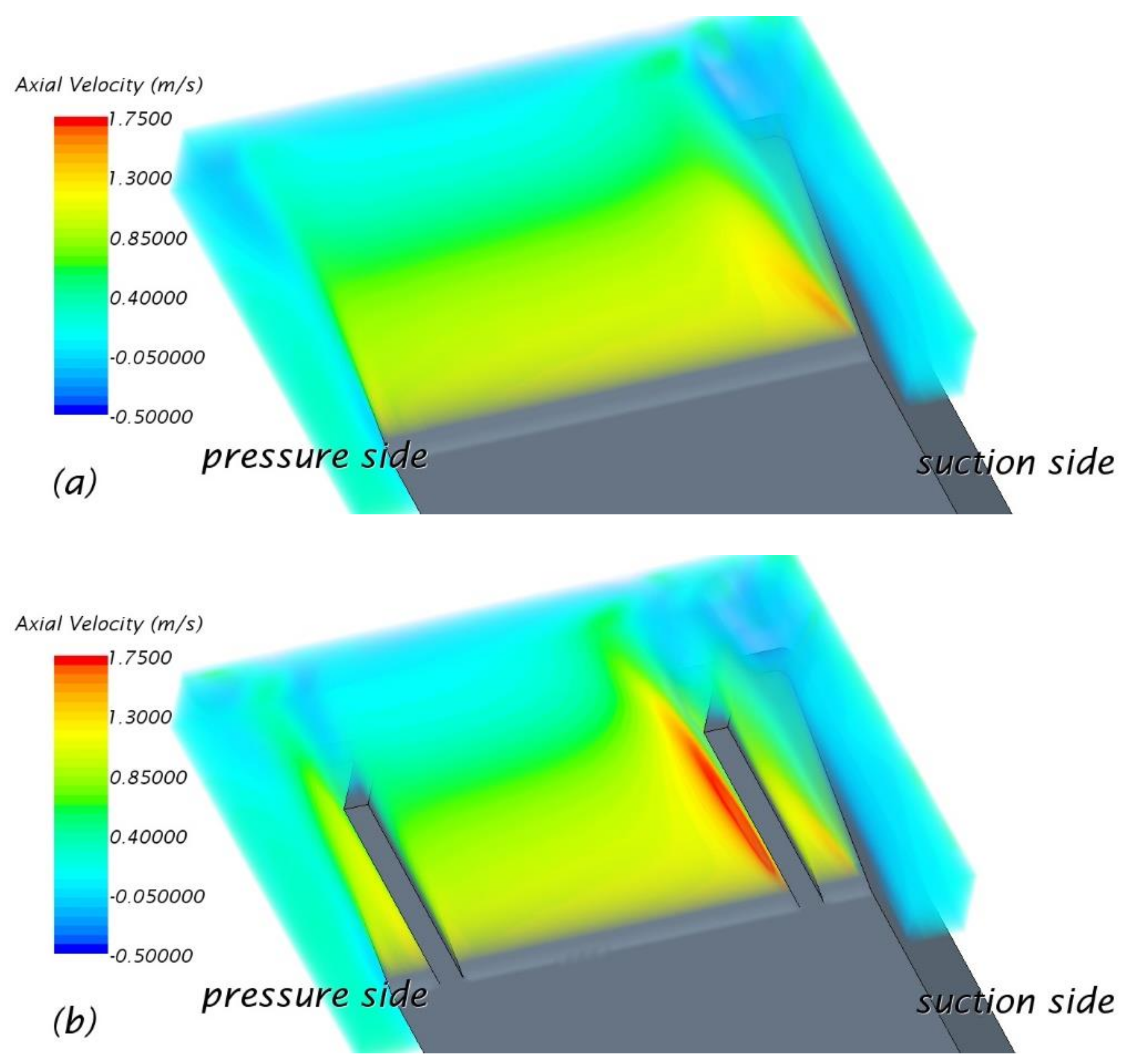
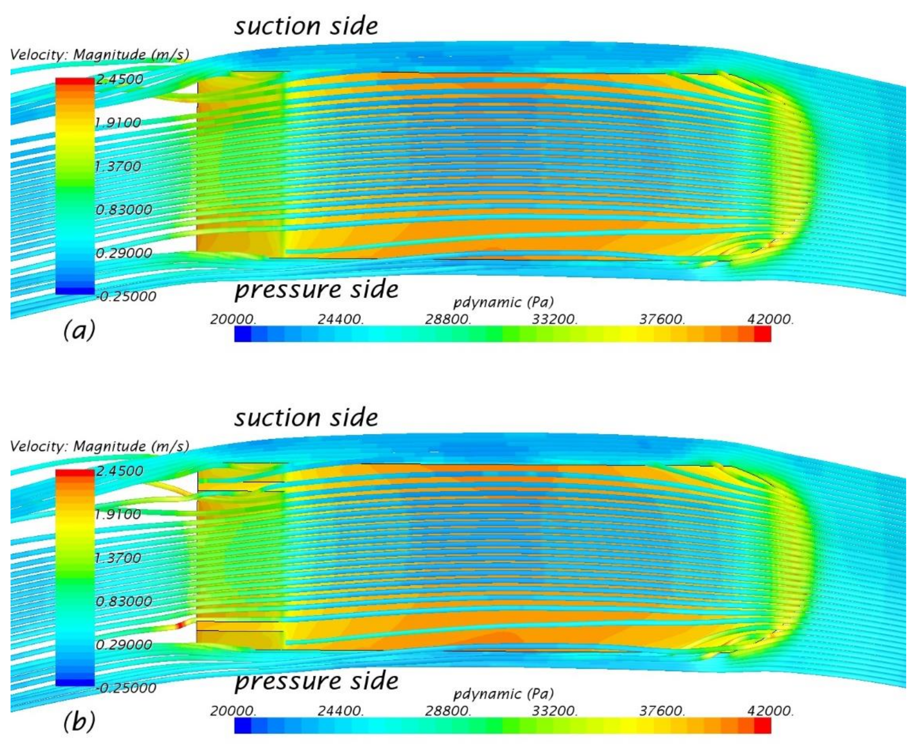
Figure 9 and Figure 10 show the axial velocity, pressure distribution, and streamline of the barge in the cases where the skeg was not installed and where they were installed, respectively. The 3D axial velocity is shown in the range of −0.32L to −0.58L from the midship. The pressure distribution on the hull surface by subtracting the hydrostatic pressure component is shown in Figure 10. The pressure side is the port side of the barge that directly receives the fluid flow, and the suction side is the starboard side, which is on the opposite side of the port.
As shown in Figure 9 and Figure 10, it can be seen that the axial velocity of the flow is rapid owing to the shedding of the aft-body side vortex at the end of the raked stern on the pressure side when the skeg is not installed. However, when the skeg is installed, it can be seen that the axial velocity is accelerating both outside the suction side skeg and inside the pressure side skeg. Analyzing the raked stern of the suction side (Figure 10), the streamline that has passed rapidly over the main bottom end is gradually slowing down towards the aft peak. This change in velocity causes the pressure distribution on the raked stern to form like a staircase. This distribution shows that the pressure increases from the pressure side skeg to the suction side skeg. It is estimated that the pressure distribution is changed by the flow velocity, and the modified pressure acts on the suction side skeg to reduce the negative yaw moment value. Such a change in the flow field seems to improve the directional stability by directing the stern to the starboard side.
3.4. Pure Yaw Simulation
Figure 11 shows the PMM test results for pure yaw simulation. In order to make it easier to understand the various wave conditions, the wave patterns are shown in Figure 11 under each condition of still water, and . The locations of the barge during the simulation were , , and . Here, is the cycle of the PMM test. Figure 11 shows the result of a case where . As indicated in the figure, it is estimated that captive sinusoidal motion is well realized.
The nondimensionalized sway force () and yaw moment () at each angular velocity of the barge are shown in Figure 12 and Figure 13.
As shown in the figure, as the angular velocity increases, the negative value of the sway force gradually increases when the skeg is not installed, while the positive value of the sway force increases when the skeg is installed. When the skeg is not installed, the sway force acting on the bow part is larger than the force acting on the stern part during turning with the angular velocity , so the negative value is indicated. However, when the skeg is installed, the sway force acting on the stern part is larger than the force acting on the bow part due to the skeg effect, and it seems that the sign becomes the positive value with the opposite sign. In this study, the simulation was conducted on a barge with round bow shape. If the bow shape is a box type, different results are expected. In the future, a comparative study will be conducted on barges with different bow shapes. Furthermore, the sway force showed a slight difference, depending on the wavelength. That is, when the skeg was not installed, it showed the smallest value in the still water and the short wavelength region and the largest value in the long wavelength region. However, when the skeg was installed, it showed the largest sway force in the still water and the smallest sway force in the long wavelength region. It was found that the negative value in the yaw moment was significantly increased when the skeg was installed, compared to the case when the skeg was not installed. In addition, in the case of the pure yaw simulation, a rapid change in fluid flow appeared from the ship’s bow and stern direction during changing yaw angle. The changing flow pattern results in unstable prediction [21]. It is noted that a study on CFD analysis with high mesh resolution in low time step needs to be carried out.
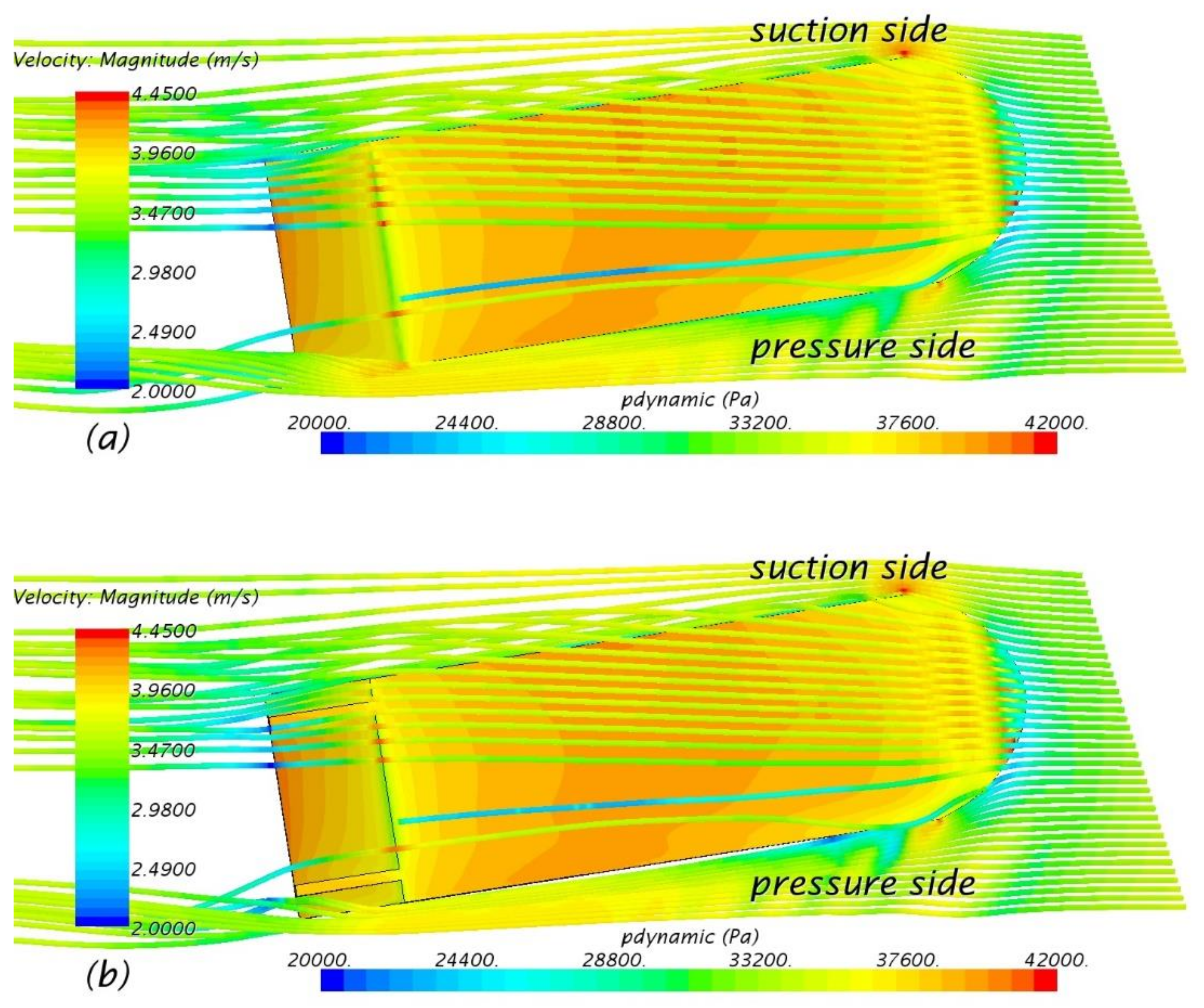
Figure 14 and Figure 15 show the axial velocity, pressure distribution, and streamline for the barge when the skeg was not installed and when they were installed, respectively. The pressure side is the port side of the barge that directly receives the fluid flow, and the suction side is the starboard side. As shown in Figure 14, when the skeg is not installed, the axial velocity shows a slightly faster distribution at the end of the suction side. However, when the skeg is installed, it is observed that the axial velocity is very fast inside the suction side skeg. The aft-body bilge flows on the pressure side are observed to be shedding without moving into the raked stern. On the other hand, the aft-body bilge flows on the suction side can be seen moving over the raked stern and moving out to the aft peak. Because of such a change in the flow velocity, the pressure distribution is modified and finally the negative yaw moment value increases.
3.5. Analysis of Directional Stability
The equation for evaluating the directional stability index that is derived from the maneuvering motion equation is shown in (14) [28,29].
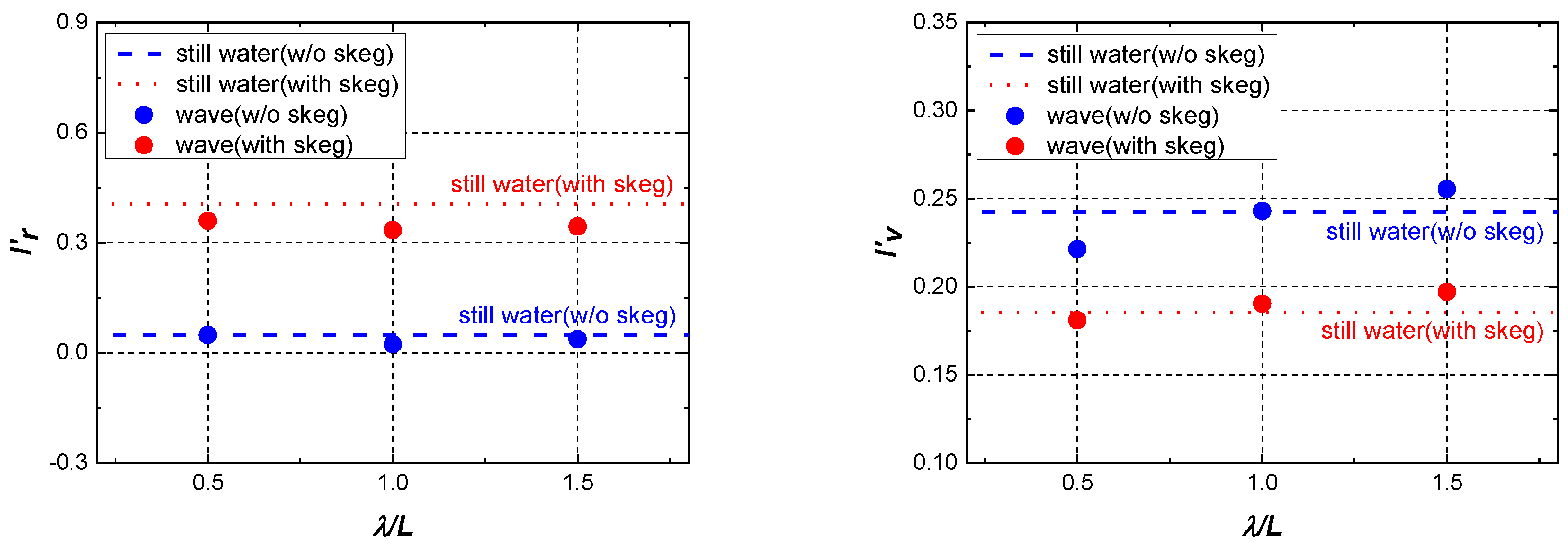
where denotes the nondimensionalized mass. In this equation, the first term indicates the yaw damping lever value (, and the second term indicates the sway damping lever (. If the yaw damping lever term increases and the sway damping lever term decreases, then it indicates that the towing stability is improved. The hydrodynamic derivatives in this study were obtained using the least square method.
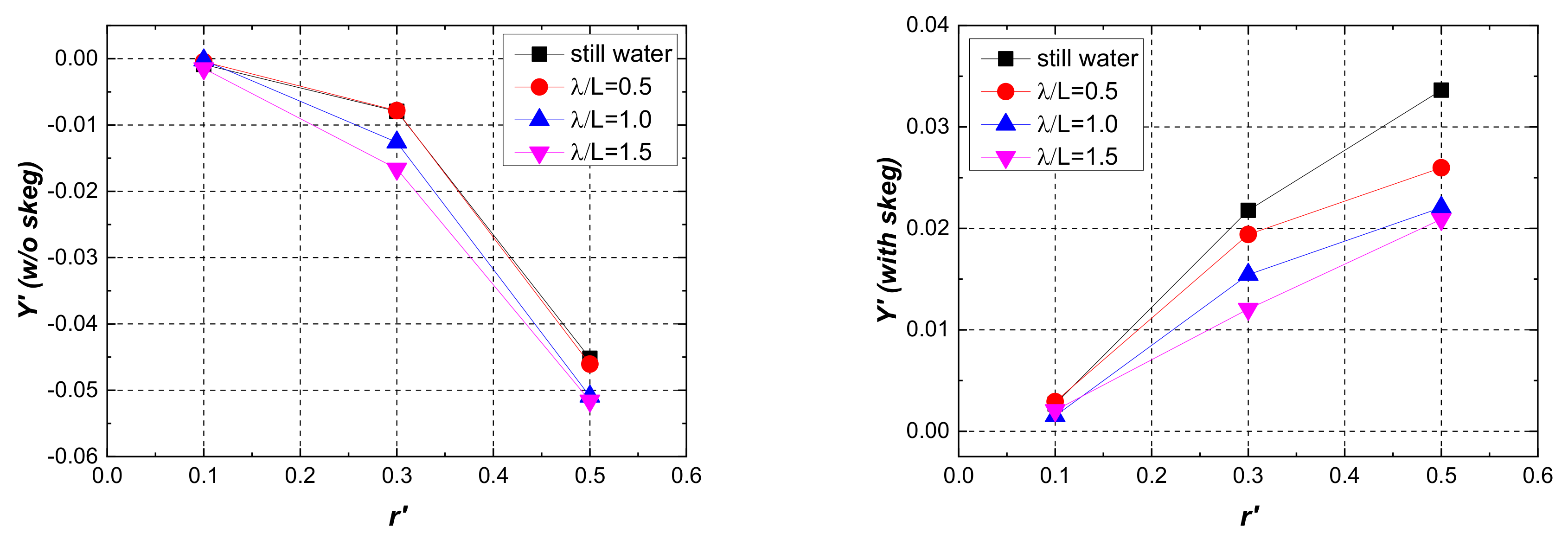
Figure 16 shows the derivative values of the maneuvering hydrodynamic forces obtained from the simulations. The blue and red colors indicate the calculation results for when the skeg was not installed and when they were installed, respectively. was slightly affected by the skeg, but decreased both in still water and in waves because of the skeg. This change in yaw moment directly caused the sway damping lever to decrease (Figure 17), resulting in the increase of the directional stability index. Because of the skeg, the sway damping lever value is reduced by 23.6% in still water, 18.2% in the short wavelength region (), 21.6% in the region where the wavelength is equal to the length of the barge (), and 22.8% in the long wavelength region ().
Next, for the hydrodynamic derivatives calculated from the pure yaw motion, shows positive and negative values, respectively, because of the effect of the skeg. shows all negative values, but the value increased owing to the installation of the skeg. It can be seen that the yaw damping lever value is greatly increased because of the skeg effect in still water and waves.
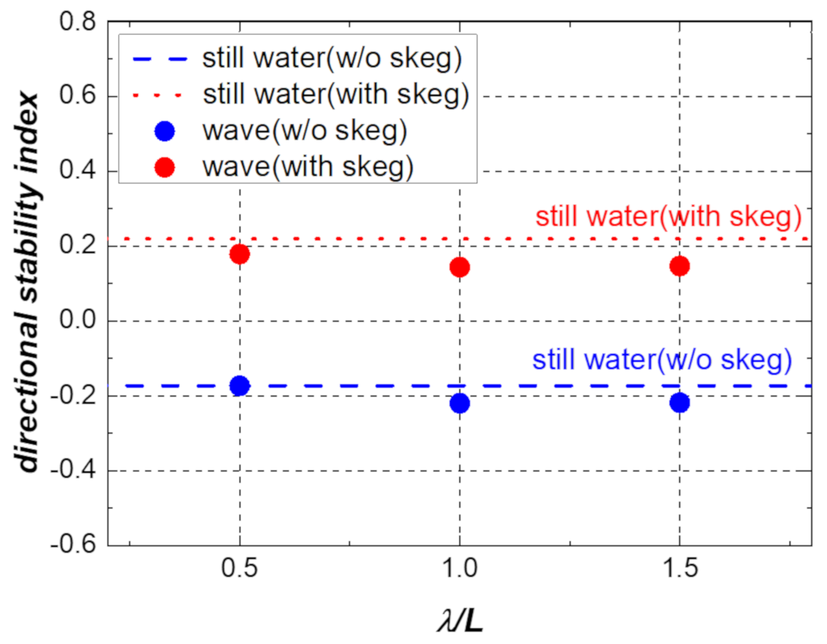
Finally, Figure 18 shows the directional stability index in still water and waves, where it is found that the directional stability of the barge is generally improved when the skeg is installed. Thus, the effect of skeg on the directional stability is very large, regardless of the influence of the wave. It was found that the directional stability somewhat decreased in waves compared to still water, regardless of whether the skeg was installed or not. In particular, as the directional stability is relatively worse in the long wavelength region than the short wavelength region, the operation of the barge requires special attention in this condition.
4. Conclusions
This study estimated the navigational safety of a barge in still water and head waves using CFD. The hydrodynamic force acting on the barge was calculated for each drift angle and angular velocity, and the flow field was simulated to comprehensively study the effect of skeg on the barge’s directional stability and wave drift force.
To summarize the contents related to the wave drift force, the steady sway force is largest in the short wavelength region, and the steady yaw moment does not show a clear tendency. The steady surge force and steady sway force are found to decrease due to the skeg effect in both short and long wavelength areas. The overall steady yaw moment tends to be reduced by the skeg.
As the drift angle increased, the sway force and yaw moment also increased. The changing trend in the sway force according to the angular velocity was different, depending on the installation of the skeg, and it was noted that the yaw moment value significantly increased because of the skeg. Because of the effect of the skeg installed on the barge, the yaw damping lever became larger, while the sway damping lever became smaller. Therefore, it was confirmed that the directional stability was improved both in still water and waves.
By understanding the effect of skeg on barge in still water and waves and considering their effect on the wave drift force and directional stability characteristics of barge, it is anticipated that the study will contribute to increasing the safety of barges by establishing comprehensive countermeasures and providing an effective response system to those who deal with actual marine navigation. We plan to verify the more common skeg effect by conducting the research on other shapes of barges.
Author Contributions
Conceptualization, C.L. and S.L.; software, S.L.; validation, C.L.; writing—original draft preparation, S.L.; writing—reviewing and editing, C.L.; supervision, S.L. All authors have read and agreed to the published version of the manuscript.
Funding
This research was supported by Basic Science Research Program through the National Research Foundation of Korea (NRF) funded by the Ministry of Education (2017R1D1A3B03030193).
Conflicts of Interest
The authors declare no conflict of interest.
References
- Inoue, S.; Kijima, K.; Doi, M. On the course stability of a barge. Trans. West Jpn. Soc. Nav. Arch. 1977, 54, 193–201. [Google Scholar]
- Chun, H.H.; Kwon, S.H.; Ha, D.D.; Ha, S.U. An experimental study on the course-keeping of an 8,000DWT barge ship. J. Soc. Nav. Arch. Korea 1997, 34, 1–11. [Google Scholar]
- Lee, S.; Lee, S.M. Experimental study on the towing stability of barges based on bow shape. J. Korean Soc. Mar. Environ. Saf. 2016, 22, 800–806. [Google Scholar] [CrossRef]
- Im, N.K.; Lee, S.M.; Lee, C.K. The influence of skegs on course stability of a barge with a different configuration. Ocean Eng. 2015, 97, 165–174. [Google Scholar] [CrossRef]
- Miyazaki, H.; Tsukada, Y.; Ueno, M. Numerical study of hydrodynamic force of manoeuvring motion about different stern form. Proc. Jpn. Soc. Nav. Archit. Ocean Eng. 2008, 7E, 17–18. [Google Scholar]
- Yasukawa, H.; Yoshimura, Y. Introduction of MMG standard method for ship maneuvering predictions. J. Mar. Sci. Technol. 2015, 20, 37–52. [Google Scholar] [CrossRef] [Green Version]
- Hirano, M.; Takashina, J.; Takeshi, K.; Saruta, T. Ship turning trajectory in regular waves. Trans. West Jpn. Soc. Nav. Arch. 1980, 60, 17–31. [Google Scholar]
- Ueno, M.; Nimura, T.; Miyazaki, H. Experimental study on manoeuvring motion of a ship in waves. In Proceedings of the International Conference on Marine Simulation and Ship Manoeuvrability, Kanazawa, Japan, 25–28 August 2003. [Google Scholar]
- Yasukawa, H. Simulation of ship maneuvering in waves (1st report: Turning motion). J. Jpn. Soc. Nav. Arch. Ocean Eng. 2006, 4, 127–136. [Google Scholar] [CrossRef] [Green Version]
- Yasukawa, H. Simulation of ship maneuvering in waves (2nd report: Zig-zag and stopping maneuvers). J. Jpn. Soc. Nav. Arch. Ocean Eng. 2008, 7, 163–170. [Google Scholar] [CrossRef] [Green Version]
- Kim, D.J.; Yun, K.H.; Park, J.Y.; Yeo, D.J.; Kim, Y.G. Experimental investigation on turning characteristics of KVLCC2 tanker in regular waves. Ocean Eng. 2019, 175, 197–206. [Google Scholar] [CrossRef]
- Tello Ruiz, M.; Mansuy, M.; Delefortrie, G.; Vantorre, M. Modelling the manoeuvring behaviour of an ULCS in coastal waves. Ocean Eng. 2019, 172, 213–233. [Google Scholar] [CrossRef]
- Skejic, R.; Faltinsen, O.M. A unified seakeeping and maneuvering analysis of ships in regular waves. J. Mar. Sci. Technol. 2008, 13, 371–394. [Google Scholar] [CrossRef]
- Seo, M.G.; Kim, Y. Numerical analysis on ship maneuvering coupled with ship motion in waves. Ocean Eng. 2011, 38, 1934–1945. [Google Scholar] [CrossRef]
- Zhang, W.; Zou, Z.J.; Deng, D.H. A study on prediction of ship maneuvering in regular waves. Ocean Eng. 2017, 137, 367–381. [Google Scholar] [CrossRef]
- Chillcce, G.; el Moctar, O. A numerical method for manoeuvring simulation in regular waves. Ocean Eng. 2018, 170, 434–444. [Google Scholar] [CrossRef]
- Tezdogan, T.; Demirel, Y.K.; Kellett, P.; Khorasanchi, M.; Incecik, A.; Turan, O. Full-scale unsteady RANS CFD simulations of ship behaviour and performance in head seas due to slow steaming. Ocean Eng. 2015, 97, 186–206. [Google Scholar] [CrossRef] [Green Version]
- Sung, Y.J.; Park, S.H. Prediction of ship manoeuvring performance based on virtual captive model tests. J. Soc. Nav. Arch. Korea 2015, 52, 407–417. [Google Scholar] [CrossRef] [Green Version]
- International Towing Tank Conference (ITTC). Practical guidelines for ship CFD applications. In Proceedings of the 26th ITTC, Rio de Janeiro, Brazil, 28 August–3 September 2011. [Google Scholar]
- User Guide STAR-CCM+; Version 10.02; CD-Adapco: Melville, NY, USA, 2015.
- Kim, H.; Akimoto, H.; Islam, H. Estimation of the hydrodynamic derivatives by RaNS simulation of planar motion mechanism test. Ocean Eng. 2015, 108, 129–139. [Google Scholar] [CrossRef]
- Park, S.H.; Oh, G.H.; Rhee, S.H.; Koo, B.Y.; Lee, H.S. Full scale wake prediction of an energy saving device by using computational fluid dynamics. Ocean Eng. 2015, 101, 254–263. [Google Scholar] [CrossRef]
- Demirel, Y.K.; Turan, O.; Incecik, A. Predicting the effect of biofouling on ship resistance using CFD. Appl. Ocean Res. 2017, 62, 100–118. [Google Scholar] [CrossRef] [Green Version]
- Celik, I.B.; Ghia, U.; Roache, P.J.; Freitas, C.J.; Coleman, H.; Raad, P.E. Procedure for estimation and reporting of uncertainty due to discretization in CFD applications. J. Fluids Eng. 2008, 130, 078001-1-4. [Google Scholar]
- Lyu, W.; el Moctar, O. Numerical and experimental investigations of wave-induced second order hydrodynamic loads. Ocean Eng. 2017, 131, 197–212. [Google Scholar] [CrossRef]
- Hizir, O.; Kim, M.; Turan, O.; Day, A.; Incecik, A. Numerical studies on non-linearity of added resistance and ship motions of KVLCC2 in short and long waves. Int. J. Nav. Arch. Ocean. Eng. 2019, 11, 143–153. [Google Scholar] [CrossRef]
- Faltinsen, O.M. Sea Loads on Ships and Offshore Structures; Cambridge University Press: Cambridge, UK, 1998. [Google Scholar]
- Lewis, E.V. Principles of Naval Architecture, 2nd ed.; The Society of Naval Architects and Marine Engineers: Jersey City, NJ, USA, 1989. [Google Scholar]
- International Towing Tank Conference (ITTC). The manoeuvring committee—final report and recommendations to the 23rd ITTC. In Proceedings of the 23rd ITTC, Venice, Italy, 8–14 September 2002. [Google Scholar]
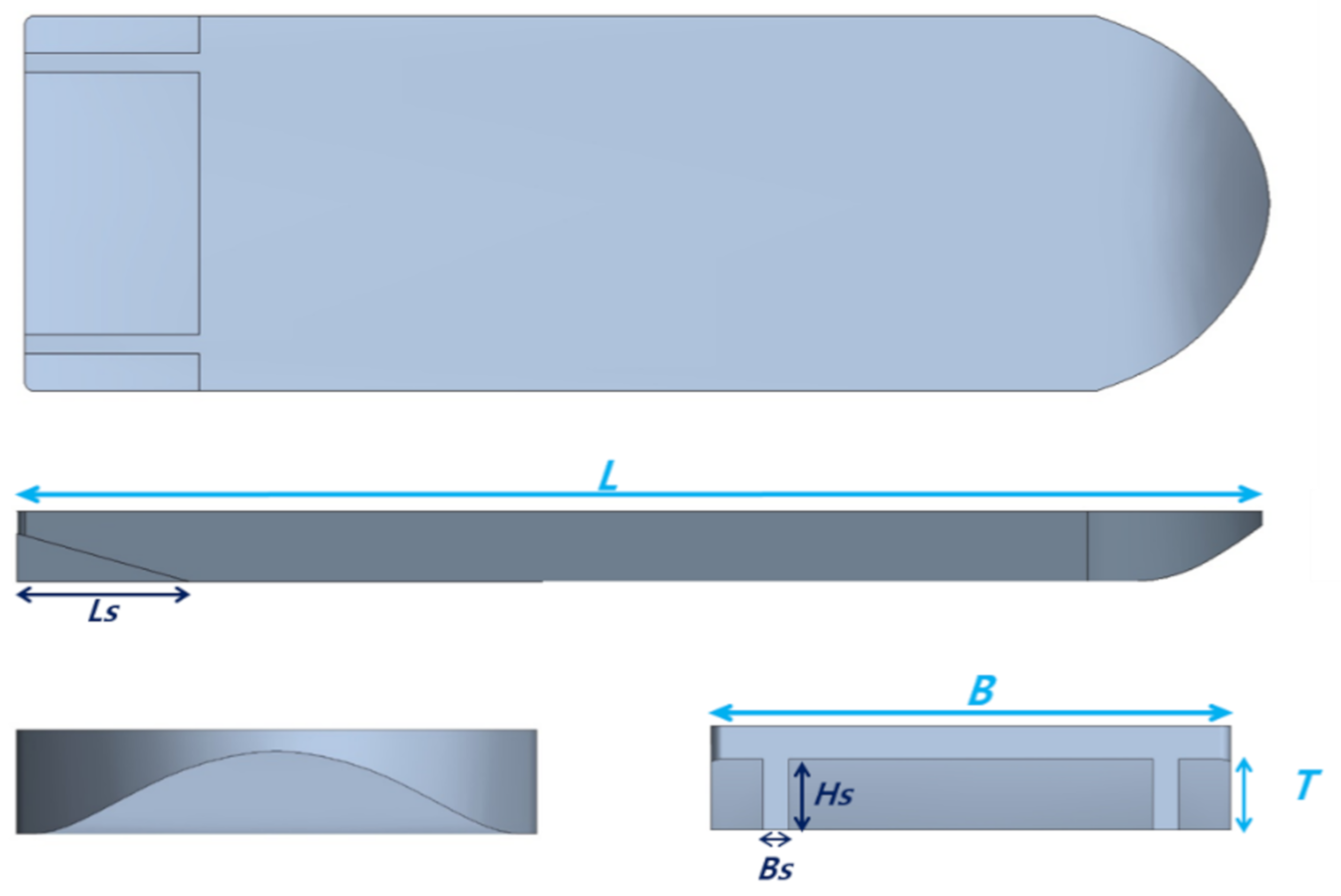
Figure 1.
Shapes of barge model.

Figure 2.
Coordinate system (left) and computational domain (right).

Figure 3.
(a) Steady surge force; (b) steady sway force; (c) steady yaw moment according to wavelength at .
Figure 3.
(a) Steady surge force; (b) steady sway force; (c) steady yaw moment according to wavelength at .


Figure 4.
Time history of sway force (left) and yaw moment (right) for still water and without skeg.
Figure 4.
Time history of sway force (left) and yaw moment (right) for still water and without skeg.

Figure 5.
Time history of sway force (left) and yaw moment (right) for still water and with skeg.

Figure 6.
Sway force in drift motion for barge without skeg (left) and with skeg (right).

Figure 7.
Yaw moment in drift motion for barge without skeg (left) and with skeg (right).

Figure 8.
Wave patterns at : (a) still water; and (b) .

Figure 9.
Axial velocity for barge at , : (a) without skeg; and (b) with skeg.


Figure 10.
Streamline and pressure distribution for barge at , : (a) without skeg; and (b) with skeg.
Figure 10.
Streamline and pressure distribution for barge at , : (a) without skeg; and (b) with skeg.

Figure 11.
Wave patterns around the barge at : (a) , still water; (b) , and; (c) , ; (d) , .


Figure 12.
Sway force in pure yaw motion for barge without skeg (left) and with skeg (right).

Figure 13.
Yaw moment in pure yaw motion for barge without skeg (left) and with skeg (right).

Figure 14.
Axial velocity for barge at , : (a) without skeg; and (b) with skeg.

Figure 15.
Streamline and pressure distribution for barge at , : (a) without skeg; and (b) with skeg.
Figure 15.
Streamline and pressure distribution for barge at , : (a) without skeg; and (b) with skeg.

Figure 16.
Hydrodynamic derivatives.

Figure 17.
Yaw damping lever (left) and sway damping lever (right).

Figure 18.
Directional stability index of barge without skeg and with skeg.


Table 1.
Main specifications of the barge.
| Description | Full Scale |
|---|---|
| Length between perpendiculars, L (m) | 91.5 |
| Breadth, B (m) | 27.5 |
| Draft, T (m) | 4.0 |
| Volume, (m3) | 10,846.0 |
| Block coefficient, CB | 0.923 |
| Length of skeg, Ls (m) | 12.810 |
| Breadth of skeg, Bs (m) | 1.375 |
| Height of skeg, Hs (m) | 3.766 |
Table 2.
Test conditions for planar motion mechanism (PMM) simulation.
| Static Drift Simulation | |||||
| Drift Angle, | Wavelength, | Wave Amplitude, | Hydrodynamic Derivatives | ||
| (-) | (deg) | (L) | (m) | (-) | |
| 0.12 | 5, 10, 15 | 0.5, 1.0, 1.5 | 0.5 | , | |
| Pure Yaw Simulation | |||||
| Angular | Lateral | Wave- | Wave | Hydrodynamic | |
| Velocity, | Displacement | length, | Amplitude, | Derivatives | |
| (-) | (-) | (m) | (L) | (m) | (-) |
| 0.12 | 0.1, 0.3, 0.5 | 100.0 | 0.5, 1.0, 1.5 | 0.5 | , |
Table 3.
Mesh numbers for each mesh configuration.
| Mesh Configuration | Total No. of Cells |
|---|---|
| Coarse | 894,673 |
| Medium | 1,549,265 |
| Fine | 3,542,882 |
Table 4.
Grid convergence study for Y and N at , .
| Y (N) | N (N·m) | |
|---|---|---|
| −78,122.5 | −3,206,399.7 | |
| −79,280.9 | −3,244,955.9 | |
| −82,076.5 | −3,290,778.9 | |
| 0.414 | 0.841 | |
| 2.542 | 0.498 | |
| −77,302.9 | −3,001,826.2 | |
| 3.53% | 1.41% | |
| 2.56% | 8.09% | |
| 3.12% | 9.37% |
Table 5.
Comparison of , , and at in still water.
| Without Skeg | With Skeg | |
|---|---|---|
| 0.07768 | 0.08098 | |
| −0.13355 | −0.13915 | |
| −0.03873 | −0.02914 |
Publisher’s Note: MDPI stays neutral with regard to jurisdictional claims in published maps and institutional affiliations. |
© 2020 by the authors. Licensee MDPI, Basel, Switzerland. This article is an open access article distributed under the terms and conditions of the Creative Commons Attribution (CC BY) license (http://creativecommons.org/licenses/by/4.0/).
Share and Cite
MDPI and ACS Style
Lee, C.; Lee, S. Effect of Skeg on the Wave Drift Force and Directional Stability of a Barge Using Computational Fluid Dynamics. J. Mar. Sci. Eng. 2020, 8, 844. https://doi.org/10.3390/jmse8110844
AMA Style
Lee C, Lee S. Effect of Skeg on the Wave Drift Force and Directional Stability of a Barge Using Computational Fluid Dynamics. Journal of Marine Science and Engineering. 2020; 8(11):844. https://doi.org/10.3390/jmse8110844
Chicago/Turabian StyleLee, Chunki, and Sangmin Lee. 2020. "Effect of Skeg on the Wave Drift Force and Directional Stability of a Barge Using Computational Fluid Dynamics" Journal of Marine Science and Engineering 8, no. 11: 844. https://doi.org/10.3390/jmse8110844
Note that from the first issue of 2016, this journal uses article numbers instead of page numbers. See further details here.