Parameter Estimation and Hypothesis Testing of Multivariate Poisson Inverse Gaussian Regression

Abstract

Multivariate Poisson regression is used in order to model two or more count response variables. The Poisson regression has a strict assumption, that is the mean and the variance of response variables are equal (equidispersion). Practically, the variance can be larger than the mean (overdispersion). Thus, a suitable method for modelling these kind of data needs to be developed. One alternative model to overcome the overdispersion issue in the multi-count response variables is the Multivariate Poisson Inverse Gaussian Regression (MPIGR) model, which is extended with an exposure variable. Additionally, a modification of Bessel function that contain factorial functions is proposed in this work to make it computable. The objective of this study is to develop the parameter estimation and hypothesis testing of the MPIGR model. The parameter estimation uses the Maximum Likelihood Estimation (MLE) method, followed by the Newton–Raphson iteration. The hypothesis testing is constructed using the Maximum Likelihood Ratio Test (MLRT) method. The MPIGR model that has been developed is then applied to regress three response variables, i.e., the number of infant mortality, the number of under-five children mortality, and the number of maternal mortality on eight predictors. The unit observation is the cities and municipalities in Java Island, Indonesia. The empirical results show that three response variables that are previously mentioned are significantly affected by all predictors.

1. Introduction

The relationship between predictor variables and Poisson distributed response variables can be analyzed while using Poisson regression. However, some cases cannot deal with the assumption in Poisson regression, namely equidispersion, which indicates that the mean is equal to the variance of the response variable. In real data, the variance can be larger than the mean (overdispersion). Thus, a proper model for analyzing such a kind of data needs to be developed. Multivariate data consists of two or more correlated response variables. The researchers have conducted several studies in the univariate Poisson regression, but the development of multivariate Poisson regression is still lacking [1].

The Poisson Inverse Gaussian Regression (PIGR) model is one of the alternative models to overcome the overdispersion issue. This model is built from mixed Poisson distribution, which is a combination of the Poisson distribution and the inverse Gaussian distribution. The PIG distribution was firstly introduced by Holla in 1996, with the characteristics of count data having a high initial value and considerably skewed to the right curve [2]. The univariate IGPR models have been widely utilized in previous studies [3,4,5,6,7,8]. Otherwise, there are few studies of the Multivariate Poisson Inverse Gaussian Regression (MPIGR) model. Ghitany et al. (2012) previously discussed research on the MPIGR model. That study examined several multivariate mixed Poisson regression models and their application. Parameter estimation was done using the MLE method by the Expectation and Maximization (EM) algorithm [9].

This study extends the MPIGR model by adding an exposure variable. Furthermore, the third modification of Bessel function contain factorial functions which results very large numbers that is incomputable by a computer. The results that cause the programming cannot be completed and the parameter estimator is not obtained. Therefore, the factorial function must be modified into a simpler form so that it does not produce incomputable numbers. Once the model specification has been determined, this research discusses the parameter estimation and hypothesis testing. The MLE method, followed by the Newton–Raphson iteration, is employed for the parameter estimation in this work. The next aim is to develop the hypothesis testing using the MLRT approach that has been done in this study. The proposed MPIGR model, along with its parameter estimation and hypothesis testing, is applied in order to model the relationship of three correlated response variables and eight predictors. The three response variables are the number of infant mortality, the number of under-five children mortality, and the number of maternal mortality. The observation unit is the cities and municipalities in Java Island, Indonesia. Furthermore, the exposure variable is used as a weight for each unit of observation. The exposure variable in this research is the number of live births.

As the third objective of the Sustainable Development Goals (SDGs), infant, under-five children, and maternal mortality are estimated to decrease every year. However, in 2017 alone, the under-five children accounted for 5.4 million death, with 2.5 million death occurring in the first month of life (neonatal), 1.6 million occurring at age 1–11 months (infant), and 1.3 million at age 1–4 years. There are 118 countries that already had an under-five mortality rate below the SDG target of a mortality rate at least as low as 25 deaths per 1000 births. At the same time, approximately 50 countries need to be accelerated to achieve the SDG target by 2030. As one of low-middle income country, the under-five mortality rate in Indonesia in 2017 is 28 deaths per 1000 births for male and 22 deaths per 1000 births for female. Nevertheless, efforts to reduce mortality inequity within country should be intensified [10].

The maternal mortality ratio (MMR) is one of statistical measures of maternal mortality. MMR is the number of maternal deaths during a given time period per 100,000 live births during the same time period. MMR is considered to be low if it is less than 100, moderate if it is 100–299, high if it is 300–499, very high if it is 500–999, and extremely high if it is greater than or equal to 1000 maternal deaths per 100,000 live births. SDGs target for maternal mortality by 2030 is reducing the global MMR to less than 70 per 100,000 births, with no country having a maternal mortality rate of more than twice the global average. The MMR of Indonesia in 2017 is 177, which is categorized as moderate and must be reduced in order to achieve the SDGs target [11]. There is a relationship among maternal mortality, infant mortality, and under-five mortality. In previous study, it stated that the maternal mortality cause the infant to be more likely to die than to survive and the survival trajectory of these children is far worse than those of mothers who not die [12].

Based on the issue above, analysis of the MPIGR model is performed in order to determine the factors that influence the mortality number of infants, under-five children, and maternal in Java, Indonesia. The remaining part of this paper is constructed, as follows. Section 2 provides the material and method in more detail. Results and conclusion are addressed in the last section.

2. Materials and Methods

2.1. Multivariate Poisson Inverse Gaussian Distribution (MPIGD)

The MPIGD is a mixed Poisson distribution that consists of two or more correlated response variables. Let Y₁, Y₂, …, Y_m as the response variables with the assumption Y_j ~ Poisson (μ_j), j = 1, 2, …, m, with its mean and variance are the same or they can be written in the following regression equation:

$${\mu }_j=E\left(Y_j\left|{\mu }_j\right.\right)=Var\left(Y_j\left|{\mu }_j\right.\right)=f\left(X;\mathsf{\beta }\right)=\mathrm{Exp}\left(X\mathsf{\beta }\right).$$

(1)

which is called as equidispersion. For some cases, equidispersion is too restrictive and rarely satisfied. Oftentimes, the conditional variance will exceed the conditional mean (overdispersion), which is likely to result from positive contagion and unobserved heterogeneity. An error term ${\epsilon }_j$ is introduced to μ_j,

$$\mathrm{Exp}\left(X^T\mathsf{\beta }+{\epsilon }_j\right)={\mu }_j\mathrm{Exp}\left({\epsilon }_j\right)={\mu }_j{v}_j$$

(2)

Thus, $v{\mu }_1,\dots ,v{\mu }_m$ are the mean for each response variable now, Y_j ~ Mixed Poisson (μ_jv_j) [8,13]. The mixed Poisson distribution depends on the specific distribution of random variable V. In this study, variable V is an inverse Gaussian distributed. Hence, Y₁, Y₂, …, Y_m are Poisson inverse Gaussian distribution (PIGD), with the probability mass function (pmf) being given by [3],

$$P\left(y_1,\dots ,y_m;\mu ,\tau \right)={\displaystyle \underset{0}{\overset{\infty }{\int }}{\displaystyle \prod _{j=1}^m\frac{e^{\left(-v{\mu }_j\right)}{\left(v{\mu }_j\right)}^{y_j}}{y_j!}}g\left(v;\tau \right)dv}$$

(3)

the $g\left(v;\tau \right)$ implies the probability density function of Inverse Gaussian of random variable V [9].

$$g\left(v;\tau \right)={\left(2\pi \tau v^3\right)}^{-0,5}{e}^{-{\left(v-1\right)}^2/2\tau v},v>0$$

(4)

where $E\left(v\right)=1$ and $Var\left(V\right)=\tau$.

Based on Equation (1), the marginal of PIGD is as follows:

$$P\left(Y_1=y_1,\dots ,Y_m=y_m|\mu ,\tau \right)={\left(2z{\pi }^{-1}\right)}^{\frac{1}{2}}{e}^{\frac{1}{\tau }}{K}_s(z){\left(z\tau \right)}^{{}^{-{\displaystyle \sum _{j=1}^m{y}_j}}}{\displaystyle \prod _{j=1}^m\frac{{\left({\mu }_j\right)}^{y_j}}{y_j!}}$$

(5)

with $s={\displaystyle \sum _{j=1}^m{y}_j}-\frac{1}{2}$, $z=\frac{1}{\tau }\sqrt{1+2\tau {\displaystyle \sum _{j=1}^m{\mu }_j}}$ and $K_s\left(z\right)=K_{\left({\displaystyle \sum _{j=1}^m{y}_j}\right)-\frac{1}{2}}\frac{1}{\tau }\sqrt{1+2\tau {\displaystyle \sum _{j=1}^m{\mu }_j}}$ is the third modification of Bessel function [14]. The property of the PIGD can be found in [15,16].

2.2. Multivariate Poisson Inverse Gaussian Regression (MPIGR)

The MPIGR model is a development model from the univariate Inverse Gaussian Poisson Regression (PIGR) with two or more correlated response variables. Let (Y_i1, Y_i2, …, Y_im) ~ MPIG (vμ_ij), where $i=1,2,\dots ,n$ $\mathrm{and}j=1,2,\dots .m$ then the MPIGR model can be stated as follows:

$$\log \left(\frac{E(Y_{ij})}{q_i}\right)=x_i^T{\mathsf{\beta }}_j$$

(6)

$$E(Y_{ij})=q_i{e}^{x_i^T{\mathsf{\beta }}_j}$$

(7)

with $E(Y_{ij})={\mu }_{ij}=q_i\exp \left(x_i{}^T{\mathsf{\beta }}_j\right)$, the q_i is an exposure variable which is defined as the weight of the i-th unit observation, $x_i^T=\left[\begin{array}{cccc}\begin{array}{cc}1& x_{1i}\end{array}& x_{2i}& \begin{array}{ccc}\cdots & x_{ki}& \cdots \end{array}& x_{pi}\end{array}\right]$ is the vector of predictor variables with (p + 1) dimension on the i-th observation (i = 1, 2, …, n), ${\mathsf{\beta }}_j^T=\left[\begin{array}{cccc}{\beta }_{j0}& {\beta }_{j1}& {\beta }_{j2}& \begin{array}{cc}\begin{array}{ccc}\dots & {\beta }_{jk}& \dots \end{array}& {\beta }_{jp}\end{array}\end{array}\right]$ is a (p + 1) × 1 vector of regression coefficient associated with the j-th response variable (j = 1, 2, …, m).

3. Results

3.1. Parameter Estimation of MPIGR Model

Estimation of the MPIGR model parameters is obtained using the Maximum Likelihood Estimation (MLE) method by maximizing the likelihood function. Two parameters will be estimated, namely β_j and τ. The first step of the MLE method is by taking n random sample, $\left(Y_{i1},Y_{i2},\dots ,Y_{ij},\dots ,Y_{im},X_{1i},X_{2i},\dots ,X_{ki},\dots X_{pi}\right)$ with j = 1, 2, …, m, k = 1, 2, …, p and i = 1, 2, …, n. The joint probability density function of $Y_{i1},Y_{i2},\dots ,Y_{im}$ is:

$$f\left(y_{ij}|{\mathsf{\beta }}_j,\tau ;j=1,2,3\right)={\left(\frac{2}{\pi \tau }\right)}^{\frac{1}{2}}{e}^{\frac{1}{\tau }}{K}_{s_i}\left(z_i\right){\left(1+2\tau {\displaystyle \sum _{j=1}^3{\mu }_{ij}}\right)}^{-\frac{\left(2{\displaystyle \sum _{j=1}^3{y}_{ij}}-1\right)}{4}}{\displaystyle \prod _{j=1}^3\frac{{\mu }_{ij}{}^{y_{ij}}}{y_{ij}!}}$$

(8)

where ${\mu }_{ij}=q_i\exp \left(x_i{}^T{\mathsf{\beta }}_j\right)$. The likelihood function of Equation (8) is as below:

$$\begin{array}{ll}L({\mathsf{\beta }}_j,\tau ;j=1,2,\dots ,m)& ={\displaystyle \prod _{i=1}^{n}f\left(y_{ij}|{\mathsf{\beta }}_j,\tau ;j=1,2,\dots ,m\right)}\\ & =e^{\frac{n}{\tau }}{\left(\frac{2}{\pi }\right)}^{\frac{n}{2}}{\left(\frac{1}{\tau }\right)}^{\frac{n}{2}}{\displaystyle \prod _{i=1}^n\left(K_{s_i}\left(z_i\right){\left(1+2\tau {\displaystyle \sum _{j=1}^m{q}_i{e}^{x_i^T{\mathsf{\beta }}_j}}\right)}^{-\frac{\left(2{\displaystyle \sum _{j=1}^m{y}_{ij}}-1\right)}{4}}{\displaystyle \prod _{j=1}^m\frac{{\left(q_i{e}^{x_i^T{\mathsf{\beta }}_{ij}}\right)}^{y_{ij}}}{y_{ij}!}}\right)}\end{array}$$

(9)

The log-likelihood function from Equation (9) is:

$$\begin{array}{l}l({\mathsf{\beta }}_j,\tau ;j=1,2,\dots ,m)=\log L\left({\mathsf{\beta }}_j,\tau ,j=1,2,\dots ,m\right)\\ =\frac{n}{\tau }-\frac{n}{2}\log \tau +\frac{n}{2}\log \left(\frac{2}{\pi }\right)+{\displaystyle \sum _{i=1}^n\log \left(K_{s_i}(z_i)\right)}-{\displaystyle \sum _{i=1}^n\left(\frac{2{\displaystyle \sum _{j=1}^m{y}_{ij}}-1}{4}\right)\log \left(1+2\tau {\displaystyle \sum _{j=1}^m{q}_i{e}^{x_i{}^T{\mathsf{\beta }}_j}}\right)}\\ +\log \left({\displaystyle \sum _{i=1}^n{\displaystyle \sum _{j=1}^m{q}_i\log \left(y_{ij}\right)}}\right)+{\displaystyle \sum _{i=1}^n{\displaystyle \sum _{j=1}^m{y}_{ij}{x}_i{}^T{\mathsf{\beta }}_j}}-\log \left({\displaystyle \sum _{i=1}^n{\displaystyle \sum _{j=1}^m{y}_{ij}!}}\right)\end{array}$$

(10)

Then, Equation (10) derive to the parameter $\theta ={\left[\begin{array}{cccc}{\mathsf{\beta }}_1^T& {\mathsf{\beta }}_2^T& \begin{array}{cc}\begin{array}{ccc}\dots & {\mathsf{\beta }}_j^T& \dots \end{array}& {\mathsf{\beta }}_m^T\end{array}& \tau \end{array}\right]}^T$ and we get:

$$\begin{array}{c}\frac{\partial l\left(\mathsf{\theta }\right)}{\partial {\mathsf{\beta }}_1}={\displaystyle \sum _{i=1}^n\frac{\partial \log K_{s_i}(z_i)}{\partial {\mathsf{\beta }}_1}}-{\displaystyle \sum _{i=1}^n\left(\frac{\left(2{\displaystyle \sum _{j=1}^3{y}_{ij}}-1\right)\tau q_i{e}^{x_i{}^T{\mathsf{\beta }}_1}{x}_i{}^T}{2\left(1+2\tau {\displaystyle \sum _{j=1}^3{q}_i{e}^{x_i{}^T{\mathsf{\beta }}_j}}\right)}\right)}+{\displaystyle \sum _{i=1}^n{y}_{i1}}{x}_i{}^T\\ ={\displaystyle \sum _{i=1}^n\frac{\partial \log K_{s_i}(z_i)}{\partial {\mathsf{\beta }}_1}}-{\displaystyle \sum _{i=1}^n\left(\frac{\left(2{\displaystyle \sum _{j=1}^3{y}_{ij}}-1\right)\tau {\mu }_{i1}{x}_i{}^T}{2\left(1+2\tau {\displaystyle \sum _{j=1}^3{\mu }_{ij}}\right)}\right)}+{\displaystyle \sum _{i=1}^n{y}_{i1}}{x}_i{}^T\end{array}$$

where $\frac{\partial \log K_{{\displaystyle \sum _{j=1}^3{y}_{ij}}-\frac{1}{2}}(z_i)}{\partial {\mathsf{\beta }}_1}=\left(-\left(\sqrt{1+2\tau {\displaystyle \sum _{j=1}^3{\mu }_{ij}}}\right)M\left({\overrightarrow{y}}_i\right)+\frac{\tau \left({\displaystyle \sum _{j=1}^3{y}_{ij}}-\frac{1}{2}\right)}{\sqrt{1+2\tau {\displaystyle \sum _{j=1}^3{\mu }_{ij}}}}\right)\left(\frac{{\mu }_{i1}{x}_i{}^T}{\sqrt{1+2\tau {\displaystyle \sum _{j=1}^3{\mu }_{ij}}}}\right)$, then

$$\begin{array}{cc}\hfill \frac{\partial l\left(\mathsf{\theta }\right)}{\partial {\mathsf{\beta }}_1}& ={\displaystyle \sum _{i=1}^n\{\left(-\left(\sqrt{1+2\tau {\displaystyle \sum _{j=1}^3{\mu }_{ij}}}\right)M\left(y_i\right)+\frac{\tau \left({\displaystyle \sum _{j=1}^3{y}_{ij}}-\frac{1}{2}\right)}{\sqrt{1+2\tau {\displaystyle \sum _{j=1}^3{\mu }_{ij}}}}\right)\frac{{\mu }_{i1}{x}_i{}^T}{\sqrt{1+2\tau {\displaystyle \sum _{j=1}^3{\mu }_{ij}}}}}-\frac{\left(2{\displaystyle \sum _{j=1}^3{y}_{ij}}-1\right)\tau {\mu }_{i1}{x}_i{}^T}{2\left(1+2\tau {\displaystyle \sum _{j=1}^3{\mu }_{ij}}\right)}+{\displaystyle \sum _{j=1}^3{y}_{i1}}{x}_i{}^T\}\hfill \\ & ={\displaystyle \sum _{i=1}^n\{\left(-\frac{2\left(1+2\tau {\displaystyle \sum _{j=1}^3{\mu }_{ij}}\right)M\left(y_i\right){\mu }_{i1}{x}_i{}^T}{2\left(1+2\tau {\displaystyle \sum _{j=1}^3{\mu }_{ij}}\right)}+\frac{2\left(1+2\tau {\displaystyle \sum _{j=1}^3{\mu }_{ij}}\right)y_{i1}{x}_i{}^T}{2\left(1+2\tau {\displaystyle \sum _{j=1}^3{\mu }_{ij}}\right)}\right)}\hfill \end{array}$$

$$\frac{\partial l\left(\mathsf{\theta }\right)}{\partial {\mathsf{\beta }}_1}={\displaystyle \sum _{i=1}^n\left[y_{i1}-M\left(y_i\right){\mu }_{i1}\right]x_i{}^T}$$

(11)

with the same procedure, generally we get:

$$\frac{\partial l\left(\mathsf{\theta }\right)}{\partial {\mathsf{\beta }}_j}={\displaystyle \sum _{i=1}^n\left[y_{ij}-M\left(y_i\right){\mu }_{ij}\right]x_i{}^T}$$

(12)

Furthermore, the first derivative of the MPIGR log-likelihood function to parameter τ is formulated as below:

$$\begin{array}{cc}\hfill \frac{\partial l\left(\mathsf{\theta }\right)}{\partial \tau }& =\frac{\partial }{\partial \tau }[\frac{n}{\tau }-\frac{n}{2}\log \tau +\frac{n}{2}\log \left(\frac{2}{\pi }\right)+{\displaystyle \sum _{i=1}^n\log \left(K_{s_i}(z_i)\right)}-{\displaystyle \sum _{i=1}^n\frac{\left(2{\displaystyle \sum _{j=1}^3{y}_{ij}}-1\right)\log \left(1+2\tau {\displaystyle \sum _{j=1}^3{\mu }_{ij}}\right)}{4}}\hfill \\ & +\log \left({\displaystyle \sum _{i=1}^n{\displaystyle \sum _{j=1}^3{q}_i\log \left(y_{ij}\right)}}\right)+{\displaystyle \sum _{i=1}^n{\displaystyle \sum _{j=1}^3{y}_{ij}{x}_i{}^T{\mathsf{\beta }}_j}}-\log \left({\displaystyle \sum _{i=1}^n{\displaystyle \sum _{j=1}^3{y}_{ij}!}}\right)]\hfill \\ & =-\frac{n}{{\tau }^2}-\frac{n}{2\tau }+{\displaystyle \sum _{i=1}^n\frac{\partial \log K_{s_i}(z_i)}{\partial \tau }}-{\displaystyle \sum _{i=1}^n\frac{\left(2{\displaystyle \sum _{j=1}^3{y}_{ij}}-1\right){\displaystyle \sum _{j=1}^3{\mu }_{ij}}}{1+2\tau {\displaystyle \sum _{j=1}^3{\mu }_{ij}}}}\hfill \end{array}$$

where $\frac{\partial \log K_{s_i}(z_i)}{\partial \tau }=\frac{\left(1+\tau {\displaystyle \sum _{j=1}^3{\mu }_{ij}}\right)\left({\displaystyle \sum _{j=1}^3{y}_{ij}}-\frac{1}{2}\right)}{\tau \left(1+2\tau {\displaystyle \sum _{j=1}^3{\mu }_{ij}}\right)}+\frac{M(y_i)\left(1+\tau {\displaystyle \sum _{j=1}^3{\mu }_{ij}}\right)}{{\tau }^2}$ and we got:

$$\begin{array}{cc}\hfill \frac{\partial l\left(\mathsf{\theta }\right)}{\partial \tau }& =-\frac{n}{{\tau }^2}-\frac{n}{2\tau }-{\displaystyle \sum _{i=1}^n\frac{\left(1+\tau {\displaystyle \sum _{j=1}^3{\mu }_{ij}}\right)\left({\displaystyle \sum _{j=1}^3{y}_{ij}}-\frac{1}{2}\right)}{\tau \left(1+2\tau {\displaystyle \sum _{j=1}^3{\mu }_{ij}}\right)}}+{\displaystyle \sum _{i=1}^n\frac{M(y_i)\left(1+\tau {\displaystyle \sum _{j=1}^3{\mu }_{ij}}\right)}{{\tau }^2}}\hfill \\ & +{\displaystyle \sum _{i=1}^n\frac{\left(2{\displaystyle \sum _{j=1}^3{y}_{ij}}-1\right){\displaystyle \sum _{j=1}^3{\mu }_{ij}}}{1+2\tau {\displaystyle \sum _{j=1}^3{\mu }_{ij}}}}\hfill \\ & =-\frac{n}{2\tau }+\frac{n}{2\tau }+{\displaystyle \sum _{i=1}^n\frac{M(y_i)\left(1+\tau {\displaystyle \sum _{j=1}^3{\mu }_{ij}}\right)-1}{{\tau }^2}}-{\displaystyle \sum _{i=1}^n{\displaystyle \sum _{j=1}^3\frac{y_{ij}}{\tau }}}\hfill \end{array}$$

$$\frac{\partial l\left(\mathsf{\theta }\right)}{\partial \tau }={\displaystyle \sum _{i=1}^n\frac{M(y_i)\left(1+\tau {\displaystyle \sum _{j=1}^m{\mu }_{ij}}\right)-1}{{\tau }^2}}-{\displaystyle \sum _{i=1}^n{\displaystyle \sum _{j=1}^m\frac{y_{ij}}{\tau }}}$$

(13)

where

$$M\left(y_i\right)=\frac{1}{\sqrt{1+2\tau {\displaystyle \sum _{j=1}^m{\mu }_{ij}}}}\frac{K_{\left({\displaystyle \sum _{j=1}^m{y}_{ij}}\right)+\frac{1}{2}}(z_i)}{K_{\left({\displaystyle \sum _{j=1}^m{y}_{ij}}\right)-\frac{1}{2}}(z_i)}$$

(14)

According to [14], the third modification of Bessel function in Equation (12) can be written, as follows:

$$K_{\left({\displaystyle \sum _{j=1}^m{y}_{ij}}\right)+\frac{1}{2}}(z_i)={\left(\frac{\pi }{2z_i}\right)}^{1/2}{e}^{-z_i}{\displaystyle \sum _{m=0}^{{\displaystyle \sum _{j=1}^m{y}_{ij}}}\frac{\left\{\left({\displaystyle \sum _{j=1}^m{y}_{ij}}\right)+m\right\}!}{\left\{\left({\displaystyle \sum _{j=1}^m{y}_{ij}}\right)-m\right\}!m!}{\left(2z_i\right)}^{-m}}$$

(15)

$$K_{\left({\displaystyle \sum _{j=1}^m{y}_{ij}}\right)-\frac{1}{2}}(z_i)=K_{\left[\left({\displaystyle \sum _{j=1}^m{y}_{ij}}\right)-1\right]+\frac{1}{2}}(z_i)={\left(\frac{\pi }{2z_i}\right)}^{1/2}{e}^{-z_i}{\displaystyle \sum _{m=0}^{\left({\displaystyle \sum _{j=1}^m{y}_{ij}}\right)-1}\frac{\left\{\left[\left({\displaystyle \sum _{j=1}^m{y}_{ij}}\right)-1\right]+m\right\}!}{\left\{\left[\left({\displaystyle \sum _{j=1}^m{y}_{ij}}\right)-1\right]-m\right\}!m!}{\left(2z_i\right)}^{-m}}$$

(16)

Equations (9)–(11) equate to zero and produce non-explicit form. Hence, an iterative method needs to be applied for estimating parameters. The iterative method used is the Newton–Raphson iteration method while using the following algorithm:

▪

Step 1. Determine the initial value for parameter ${\widehat{\mathsf{\theta }}}^{\left(0\right)}={\left[\begin{array}{cccc}{\widehat{\mathsf{\beta }}}_1^{T\left(0\right)}& {\widehat{\mathsf{\beta }}}_2^{T\left(0\right)}& \begin{array}{cc}\begin{array}{ccc}\cdots & {\widehat{\mathsf{\beta }}}_j^{T\left(0\right)}& \cdots \end{array}& {\widehat{\mathsf{\beta }}}_m^{T\left(0\right)}\end{array}& {\widehat{\tau }}^{\left(0\right)}\end{array}\right]}^T$. The initial value of parameter ${\widehat{\mathsf{\theta }}}^{\left(0\right)}$ is obtained while using the separate univariate Poisson regression. The initial value for overdispersion parameter τ used the average of the observed overdispersion based on the variance of PIGD [9].

▪

Step 2. Determine the gradient vector $g\left({\widehat{\mathsf{\theta }}}^{\left(r\right)}\right)$, which is the elements consist of the first derivative of the log-likelihood function, $g^T\left({\widehat{\mathsf{\theta }}}^{\left(r\right)}\right)={\left[\begin{array}{ccc}\frac{\partial l\left(\widehat{\mathsf{\theta }}\right)}{\partial {\widehat{\mathsf{\beta }}}_1}& \begin{array}{cc}\frac{\partial l\left(\widehat{\mathsf{\theta }}\right)}{\partial {\widehat{\mathsf{\beta }}}_2}& \begin{array}{cc}\begin{array}{ccc}\cdots & \frac{\partial l\left(\widehat{\mathsf{\theta }}\right)}{\partial {\widehat{\mathsf{\beta }}}_j}& \cdots \end{array}& \frac{\partial l\left(\widehat{\mathsf{\theta }}\right)}{\partial {\widehat{\mathsf{\beta }}}_m}\end{array}\end{array}& \frac{\partial l\left(\widehat{\mathsf{\theta }}\right)}{\partial \widehat{\tau }}\end{array}\right]}_{\widehat{\mathsf{\theta }}={\widehat{\mathsf{\theta }}}_{(t)}}$.

▪

Step 3. Determine the Hessian matrix $H\left({\widehat{\mathsf{\theta }}}^{\left(r\right)}\right)$ where the elements consist of the second derivative of the log-likelihood function, as follows

$$H\left({\widehat{\mathsf{\theta }}}^{\left(r\right)}\right)=\left[\begin{array}{cccccc}\frac{{\partial }^{2}l\left(\widehat{\mathsf{\theta }}\right)}{\partial {\widehat{\mathsf{\beta }}}_1\partial {\widehat{\mathsf{\beta }}}_1^T}& \cdots & \frac{{\partial }^{2}l\left(\widehat{\mathsf{\theta }}\right)}{\partial {\widehat{\mathsf{\beta }}}_1\partial {\widehat{\mathsf{\beta }}}_j^T}& \cdots & \frac{{\partial }^{2}l\left(\widehat{\mathsf{\theta }}\right)}{\partial {\widehat{\mathsf{\beta }}}_1\partial {\widehat{\mathsf{\beta }}}_m^T}& \frac{{\partial }^{2}l\left(\widehat{\mathsf{\theta }}\right)}{\partial {\widehat{\mathsf{\beta }}}_1\partial \widehat{\tau }}\\ & \ddots & ⋮& ⋮& ⋮& ⋮\\ & & \frac{{\partial }^{2}l\left(\widehat{\mathsf{\theta }}\right)}{\partial {\widehat{\mathsf{\beta }}}_j\partial {\widehat{\mathsf{\beta }}}_j^T}& \cdots & \frac{{\partial }^{2}l\left(\widehat{\mathsf{\theta }}\right)}{\partial {\widehat{\mathsf{\beta }}}_j\partial {\widehat{\mathsf{\beta }}}_m^T}& \frac{{\partial }^{2}l\left(\widehat{\mathsf{\theta }}\right)}{\partial {\widehat{\mathsf{\beta }}}_j\partial \widehat{\tau }}\\ & & & \ddots & & \\ & & & & \frac{{\partial }^{2}l\left(\widehat{\mathsf{\theta }}\right)}{\partial {\widehat{\mathsf{\beta }}}_m\partial {\widehat{\mathsf{\beta }}}_m^T}& \frac{{\partial }^{2}l\left(\widehat{\mathsf{\theta }}\right)}{\partial {\widehat{\mathsf{\beta }}}_m\partial \widehat{\tau }}\\ symmetric& & & & & \frac{{\partial }^{2}l\left(\widehat{\mathsf{\theta }}\right)}{\partial {\widehat{\tau }}^2}\end{array}\right]$$

▪

Step 4. Start the Newton–Raphson iteration using the following formula,

$${\widehat{\mathsf{\theta }}}^{(r+1)}={\widehat{\mathsf{\theta }}}^{(r)}-H^{-1}\left({\widehat{\mathsf{\theta }}}^{(r)}\right)g\left({\widehat{\mathsf{\theta }}}^{(r)}\right)$$

(17)

with ${\widehat{\mathsf{\theta }}}^{\left(r\right)}={\left[\begin{array}{cccc}{\widehat{\mathsf{\beta }}}_1^T& {\widehat{\mathsf{\beta }}}_2^T& \begin{array}{cc}\begin{array}{ccc}\cdots & {\widehat{\mathsf{\beta }}}_j^T& \cdots \end{array}& {\widehat{\mathsf{\beta }}}_m^T\end{array}& \widehat{\tau }\end{array}\right]}^T$ and r = 0, 1, 2, …, r*.

▪

Step 5. The iteration will stop if $‖{\widehat{\mathsf{\theta }}}^{\left(r+1\right)}-{\widehat{\mathsf{\theta }}}^{\left(r\right)}‖\le \epsilon$, with ε is a very small value and it will produce the estimator value for each parameter.

3.2. Factorial Simplification in the Third Modification of BESSEL Function

The factorial function in the third modification of Bessel function, as performed in Equations (15) and (16) results in the large value by the calculation in programming. These results cause the program unable to complete, so that parameter estimates cannot be obtained. Therefore, the factorial simplification in Bessel function is needed. Based on Equations (15) and (16), let ${\displaystyle \sum _{j=1}^m{y}_j}=N$. Because the factorial function only works for these conditions, N > 0, m > 0, and n > m, accordingly (N + m)! contains the whole of (N−m)! and the factorial function can be simplified, as below:

$$\begin{gathered} \begin{array}{cc}\frac{\left(N+m\right)!}{\left(N-m\right)!}& =\frac{1\times 2\times 3\times \dots \times \left(N-m-1\right)\times \left(N-m\right)\times \left(N-m+1\right)\times \dots \times \left(N+m\right)}{1\times 2\times 3\times \dots \times \left(N-m-1\right)\times \left(N-m\right)}\\ & =\left(N-m+1\right)\times \left(N-m+2\right)\times \dots \times \left(N+m\right)\end{array} \\ ={\displaystyle \prod _{a=1}^{2m}\left(N-m+a\right)} \end{gathered}$$

(18)

According to Equation (18), the factorial function in Equation (15) can be written, as follows:

$${\displaystyle \sum _{m=0}^{{\displaystyle \sum _{j=1}^m{y}_j}}\frac{\left({\displaystyle \sum _{j=1}^m{y}_j}+m\right)!}{\left({\displaystyle \sum _{j=1}^m{y}_j}-m\right)!m!}}{\left(2z\right)}^{-m}={\displaystyle \sum _{m=0}^{{\displaystyle \sum _{j=1}^m{y}_j}}{\displaystyle \prod _{a=1}^{2m}\left({\displaystyle \sum _{j=1}^3{y}_j}-m+a\right)}\frac{{\left(2z\right)}^{-m}}{m!}}$$

(19)

with the same procedure, the factorial function in Equation (16) can be simplified, as below:

$${\displaystyle \sum _{m=0}^{{\displaystyle \sum _{j=1}^3{y}_j}}\frac{\left({\displaystyle \sum _{j=1}^3{y}_j}-1+m\right)!}{\left({\displaystyle \sum _{j=1}^3{y}_j}-1-m\right)!m!}}{\left(2z\right)}^{-m}={\displaystyle \sum _{m=0}^{{\displaystyle \sum _{j=1}^3{y}_j}}{\displaystyle \prod _{a=1}^{2m-1}\left({\displaystyle \sum _{j=1}^3{y}_j}-m+a\right)}\frac{{\left(2z\right)}^{-m}}{m!}}$$

(20)

Substitute Equations (19) and (20) to Equations (15) and (16) in order to calculate $M\left(y_i\right)$ in Equation (14). The result of $M\left(y_i\right)$ will be used in the first and second derivative of MPIGR log-likelihood function in order to obtain the parameter estimation.

3.3. Hypothesis Testing of MPIGR Model

The hypothesis testing of the MPIG regression model was undertaken by the Maximum Likelihood Ratio Test (MLRT) method both simultaneously and partially. Simultaneous hypothesis testing is performed in order to determine the significance of the regression parameters in the model simultaneously with the following hypothesis: the null hypothesis is β_j1 = β_j2 = … = β_jk = … = β_jp = 0 and τ = 0 and the alternative hypothesis is at least one β_jk ≠ 0 and τ ≠ 0, where j = 1, 2, …, m; and k = 1, 2,…, p.

Let Ω as a set of parameters under population with $\mathsf{\Omega }=\left\{{\mathsf{\beta }}_j,\tau ;j=1,2,\dots ,m\right\}$ and $\omega$ is a set of parameters under null hypothesis with $\omega =\left\{{\beta }_{0\omega j},{\tau }_{\omega };j=1,2,\dots ,m\right\}.$ The $L(\widehat{\mathsf{\Omega }})$ is the likelihood of the full model, which includes all of the predictor variables, and $L(\widehat{\omega })$ is the likelihood of a saturated model without predictor variables. The likelihood function for each model, as follows:

$$L\left(\mathsf{\Omega }\right)={\displaystyle \prod _{i=1}^{n}P\left(Y=y_i|x_i;\mathsf{\beta },\tau \right)}$$

(21)

and

$$\begin{array}{cc}\hfill L\left(\omega \right)& ={\displaystyle \prod _{i=1}^{n}P\left(Y=y_i|{\beta }_{0\omega },{\tau }_{\omega }\right)}\hfill \\ & =e^{\frac{n}{{\widehat{\tau }}_{\widehat{\omega }}}}{\left(\frac{2}{\pi }\right)}^{\frac{n}{2}}{\left(\frac{1}{{\widehat{\tau }}_{\widehat{\omega }}}\right)}^{\frac{n}{2}}{\displaystyle \prod _{i=1}^n\left(K_s\left(z\right){\left(1+2{\widehat{\tau }}_{\widehat{\omega }}{\displaystyle \sum _{j=1}^3{q}_i{e}^{{\widehat{\beta }}_{0\omega j}}}\right)}^{-\frac{\left(2{\displaystyle \sum _{j=1}^3{y}_{ij}}-1\right)}{4}}{\displaystyle \prod _{j=1}^3\frac{{\left(q_i{e}^{{\widehat{\beta }}_{0\omega j}}\right)}^{y_{ij}}}{y_{ij}!}}\right)}\hfill \end{array}$$

(22)

The test statistics for the hypothesis in the simultaneous test of MPIGR model is formulated, as below.

$$G^2=-2\log \left(\frac{L(\widehat{\omega })}{L(\widehat{\mathsf{\Omega }})}\right)=2\left(\log L(\widehat{\mathsf{\Omega }})-\log L(\widehat{\omega })\right)$$

(23)

The log-likelihood function in Equation (22) is maximized by determining the first-order partial derivative of the log-likelihood function with respect to the parameters of ${\beta }_{0\omega j}$ and ${\tau }_{\omega }$ and the results are as follows.

$$\frac{\partial l(\omega )}{\partial {\beta }_{0\omega 1}}={\displaystyle \sum _{i=1}^n\left[y_{i1}-M\left(y_i\right)e^{{\beta }_{0\omega 1}}\right]}$$

(24)

Generally, we get:

$$\frac{\partial l(\mathsf{\omega })}{\partial {\beta }_{0\omega j}}={\displaystyle \sum _{i=1}^n\left[y_{ij}-M\left(y_i\right)e^{{\beta }_{0\omega j}}\right]}$$

(25)

$$\frac{\partial l(\omega )}{\partial {\tau }_{\omega }}={\displaystyle \sum _{i=1}^n\left\{\frac{M\left(y_i\right)\left(1+{\tau }_{\omega }{\displaystyle \sum _{j=1}^3{q}_i{e}^{{\beta }_{0\omega j}}}\right)-1}{{\tau }_{\omega }^2}\right\}}-{\displaystyle \sum _{i=1}^n{\displaystyle \sum _{j=1}^3\frac{y_{ij}}{{\tau }_{\omega }}}}$$

(26)

Hence, the statistics G² for the MPIGR model determined by substituting Equations (9) and (22) to Equation (23) and the result is as follows:

$$\begin{array}{cc}\hfill G^2& =2[n\left(\frac{1}{\widehat{\tau }}-\frac{1}{{\widehat{\tau }}_{\widehat{\omega }}}+\frac{1}{2}\log \frac{{\widehat{\tau }}_{\widehat{\omega }}}{\widehat{\tau }}\right)+{\displaystyle \sum _{i=1}^n\log \left(\frac{K_{s_i}(z_i)}{K_{s_i}(z_{\widehat{\omega }i})}\right)}+{\displaystyle \sum _{i=1}^n\frac{\left(2{\displaystyle \sum _{j=1}^m{y}_{ij}}-1\right)}{4}}\log \left(\frac{1+2{\widehat{\tau }}_{\widehat{\omega }}{\displaystyle \sum _{j=1}^m{q}_i{e}^{{\widehat{\beta }}_{0\widehat{\omega }j}}}}{1+2\widehat{\tau }{\displaystyle \sum _{j=1}^m{q}_i{e}^{x_i{}^T{\widehat{\mathsf{\beta }}}_j}}}\right)\hfill \\ & +{\displaystyle \sum _{i=1}^n{\displaystyle \sum _{j=1}^m{y}_{ij}{x}_i{}^T{\widehat{\mathsf{\beta }}}_j}}-{\displaystyle \sum _{i=1}^n{\displaystyle \sum _{j=1}^m{y}_{ij}{\widehat{\beta }}_{0\widehat{\omega }j}}}]\hfill \end{array}$$

(27)

The details of the statistics G² based on the likelihood ratio test method is described in Appendix A. The statistics G² follows the asymptotic of the Chi-square distribution, such that the significant level α reject the null hypothesis when G² value falls into the rejection region, i.e., when $G^2>{\chi }_{\alpha ,\left(p+1\right)k}^2$.

3.4. Application

The MPIGR model in this study is applied in order to model the number of infants, child, and maternal death. The data are collected from the Health Profile of Java, Indonesia, in 2017. There are six provinces with 119 cities or municipalities in Java Island. Because of the data limitation, Banten Province was not included in this study. Thus, this study only used 111 cities or municipalities.

The variables used in this study is consist of three correlated response variables, namely the number of infant mortality (Y₁), under-five children mortality(Y₂), and maternal mortality (Y₃). There are eight predictor variables, such as the percentage of antenatal care visit by pregnant women (X₁), the percentage of pregnant women who received Fe3 tablet (X₂), the percentage of complete neonatal visits (X₃), the percentage of Low Birth Weight (LBW) (X₄), the percentage of healthy house (X₅), the percentage of active integrated service post (X₆), the percentage of infants received vitamin A (X₇), and the percentage of births that are assisted by health workers (X₈). Banten Province does not have several predictor variables selected, which is quite important for modelling the response variable. Thus, Banten Province was excluded from the study on the consideration of the selected predictor variables.

Every region in Java Island has different characteristics. Therefore, the exposure variable is needed, because the city or municipality is worth comparing. The exposure variable used in this study is the number of live births of each city or municipality in Java.

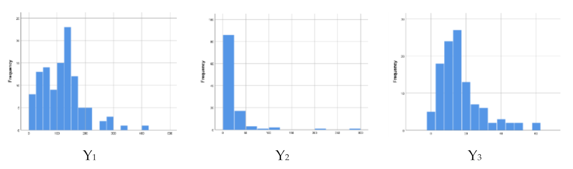
Based on

Table 1. Description of the response variables.

Variable	Mean	SD	Coefficient of Variation	Min	Max
The number of infant mortality (Y1)	118.08	72.885	63.4	7	403
The number of child mortality (Y2)	20.41	36.554	425.6	0	278
The number of maternal mortality (Y3)	16.4	12.233	89.1	0	59

, the means of three response variables are 118.08, 20.41, and 16.4. Because the mean of Y₁, Y₂, and Y₃ differ greatly, we need to measure the spread of the data. The coefficient of variation (CoV) can be used to measure data distribution. The CoV of Y₁, Y₂, and Y₃ are 63.4, 425.6, and 89.1. The number of child mortality (Y₂) has the highest CoV, which means that variable Y₂ is more heterogenous than the other two variables. This evidence is also supported by histogram for Y₁, Y₂, and Y₃ in Figure 1. It shows that the Y₂ curve is quite skewed to the right than Y₁ and Y₃.

Table 2. Descriptive statistics of predictor variables that are based on city or municipality in Java.

Variable	Province
	Jakarta	Yogyakarta	Central Java	West Java	East Java
The percentage of antenatal care visit by pregnant women	99.26 (6.10) a	90.92 (3.61)	92.86 (3.62)	97.44 (8.20)	89.34 (5.47)
The percentage of pregnant woman who received Fe3 tablet	95.14 (4.35)	88.05 (4.41)	92.85 (4.01)	95.88 (9.50)	88.37 (5.67)
The percentage of complete neonatal visits	95.44 (2.13)	77.32 (28.53)	92.97 (10.29)	94.30 (16.78)	96.34 (3.82)
The percentage of Low Birth Weight (LBW)	1.07 (1.45)	5.26 (1.14)	4.54 (0.93)	2.87 (1.66)	4.20 (1.41)
The percentage of healthy house	66.33 (18.85)	70.59 (17.97)	85.27 (14.17)	71.25 (15.84)	70.53 (16.40)
The percentage of active integrated service post	100 (0.00)	76.99 (9.36)	66.98 (18.88)	63.07 (20.58)	78.14 (14.53)
The percentage of infants received vitamin A	92.52 (8.13)	90.92 (16.40)	97.25 (8.43)	91.76 (16.01)	98.30 (7.97)
The percentage of births assisted by health workers	98.00 (5.56)	100.0 (0.00)	99.14 (1.56)	97.94 (8.39)	94.04 (4.16)
The number of live births b	34649 (23137)	8470 (4548)	15424 (7310)	33903 (25870)	15144 (10125)

a: Mean (Standard deviation); b: Exposure variable.

displays the characteristics of each predictor that is presumed to influence the number of infants, child, and maternal deaths. The characteristics of each predictor are explained based on the mean and standard deviation for each province in Java Island. As a health indicator, these predictors are expected to meet the targets in order to improve the quality of health in Indonesia.

Predictors other than LBW are expected to have a high percentage, because these predictors are thought to reduce the number of infants, child, and maternal death. In comparison, LBW is expected to have a low percentage, because LBW is believed to be able to increase the number of infant deaths.

Based on Table 2, almost all of the provinces in Java reach an average of 80–90% for some predictors, except LBW. Still, the province with a low percentage, such as Yogyakarta, has the average of the ratio of complete neonatal visits at 77.32% that should be increased. Furthermore, for the percentage of active integrated service posts, other provinces except Jakarta have a percentage of 60–78%, which is a quite low average. The active integrated service post is a form of Community-Based Health Efforts to facilitate the public for infants, children, and maternal to get health services. Aside from active integrated service posts, the percentage of healthy homes in all provinces in Java has not reached 80% other than Central Java Province. Additional suggestions to the government, the role of the community should be improved in order to encourage the people to get involved in the implementation of active integrated service posts, and the percentage of healthy homes.

The characteristics of each predictor provide a description and presumption about the predictors affect the number of infants, child, and maternal deaths in Java. Further analysis is required to obtain more accurate results. The MPIGR model is used to determine the predictors, since it significantly affects the number of infants, child, and maternal death in Java. Before applying the MPIGR, it is necessary to test the overdispersion assumption. Overdispersion occurs when the variance is higher than the mean. The overdispersion exists when the deviance value over the degree of freedom is higher than one, and the ratio of Pearson Chi-square value over the degree of freedom is higher than one.

Table 3. Overdispersion test.

Variable	Deviance	df	Deviance/df
Number of infant mortality (Y1)	4462.60	102	43.75
Number of child mortality (Y2)	2181.11	102	21.38
Number of maternal mortality (Y3)	670.05	102	6.57

shows that all of the response variables suffer overdispersion, because the values of deviance/df are higher than one. Therefore, the MPIGR model should be used to model the data. The relationship between pair of response variables was measured by the Pearson’s product–moment correlation. The coefficient of Pearson’s correlation between variable Y₁ and Y₂ is 0.543 (p-value = 6.97 × 10⁻¹⁰). The coefficient of Pearson’s correlation between variable Y₁ and Y₃ is 0.587 (p-value = 1.29 × 10⁻¹¹). Otherwise, the coefficient of Pearson’s correlation between variable Y₂ and Y₃ is 0.130 (p-value = 0.172). Even though there is one pair of the response variables that has significantly no correlation, we need to make sure whether there is dependency among the response variables in multivariate way. Therefore, we calculated the correlation using Bartlett’s test. The result shows that ${\chi }^2(92.238)>{\chi }_{3,0.05}^2(7.815)$ and p-value (7.20 × 10⁻²⁰) < α (0.05). The decision is to reject the null hypothesis, stating that Pearson correlation matrix not equal to an identity matrix. Thus, the response variable can be used in multivariate analysis while using the MPIGR model.

The significance of the simultaneous test shows that the statistics G² = 39.86 × 10⁸ is higher than ${\chi }_{0.05,25}^2=37.653$; hence, the decision to reject the null hypothesis. It means that there is at least one predictor variable that significantly influences the number of infants, child, and maternal mortality.

The partial hypothesis testing is done in order to determine the significant predictor variables that are influencing the number of infants, child, and maternal mortality in Java.

Table 4. Parameter estimation of each predictor at each response variables.

Parameter	The Number of Infant Mortality				The Number of Under-Five Children Mortality				The Number of Maternal Mortality
	Est	Se	Z	P	Est	Se	Z	P	Est	Se	Z	P
${\beta }_0$	4.101	5.27 × 10−4	−7.78 × 103	p < 0.001	−2.549	5.17 × 10−3	4.92 × 102	p < 0.001	3.613	3.59 × 10−2	−1.00 × 102	p < 0.001
${\beta }_1$	−0.032	7.40 × 10−8	4.31 × 105	p < 0.001	−0.072	7.24 × 10−7	9.89 × 104	p < 0.001	0.014	1.06 × 10−5	−1.34 × 103	p < 0.001
${\beta }_2$	0.004	6.23 × 10−8	6.16 × 104	p < 0.001	−0.018	6.15 × 10−7	−2.87 × 104	p < 0.001	0.007	3.05 × 10−6	2.31 × 103	p < 0.001
${\beta }_3$	−0.003	5.16 × 10−9	−5.33 × 105	p < 0.001	0.001	5.03 × 10−9	−2.64 × 105	p < 0.001	−0.003	4.43 × 10−8	−6.09 × 104	p < 0.001
${\beta }_4$	−0.076	6.83 × 10−7	1.11 × 105	p < 0.001	−0.449	1.41 × 10−5	3.18 × 104	p < 0.001	−0.119	3.54 × 10−5	3.36 × 103	p < 0.001
${\beta }_5$	−0.002	3.88 × 10−9	4.88 × 105	p < 0.001	0.005	2.04 × 10−8	2.24 × 105	p < 0.001	−0.005	3.99 × 10−7	1.28 × 104	p < 0.001
${\beta }_6$	−0.005	3.67 × 10−9	1.37 × 106	p < 0.001	0.019	2.53 × 10−8	−7.59 × 105	p < 0.001	−0.013	2.60 × 10−7	5.34 × 104	p < 0.001
${\beta }_7$	0.004	6.67 × 10−9	−6.03 × 105	p < 0.001	−0.005	2.02 × 10−8	−2.57 × 105	p < 0.001	0.006	8.32 × 10−7	−7.68 × 103	p < 0.001
${\beta }_8$	0.041	3.26 × 10−8	1.24 × 106	p < 0.001	0.144	1.94 × 10−6	7.42 × 104	p < 0.001	3.613	3.59 × 10−2	−1.00 × 102	p < 0.001

shows the estimation results of MPIGR model parameters.

The estimate of the dispersion parameter (τ) is 0.493 with its p < 0.001. Based on the empirical results summarized in Table 3, all of the predictor variables have a significant effect on the three responses. The MPIGR model of these three responses and eight predictors can be written in the following equations:

$$\begin{array}{c}{\widehat{\mu }}_{1i}=q_i\exp \left(4.101-0.032X_{1i}+0.004X_{2i}-0.003X_{3i}-0.076X_{4i}-0.002X_{5i}-0.005X_{6i}\right.\left.+0.004X_{7i}+0.041X_{8i}\right)\\ {\widehat{\mu }}_{2i}=q_i\exp \left(-2.549-0.072X_{1i}-0.018X_{2i}+0.001X_{3i}-0.449X_{4i}+0.005X_{5i}+0.019X_{6i}\right.\left.-0.005X_{7i}+0.144X_{8i}\right)\\ {\widehat{\mu }}_{3i}=q_i\exp \left(3.613+0.014X_{1i}+0.007X_{2i}-0.003X_{3i}-0.019X_{4i}-0.005X_{5i}-0.013X_{6i}\right.\left.+0.006X_{7i}-0.013X_{8i}\right)\end{array}$$

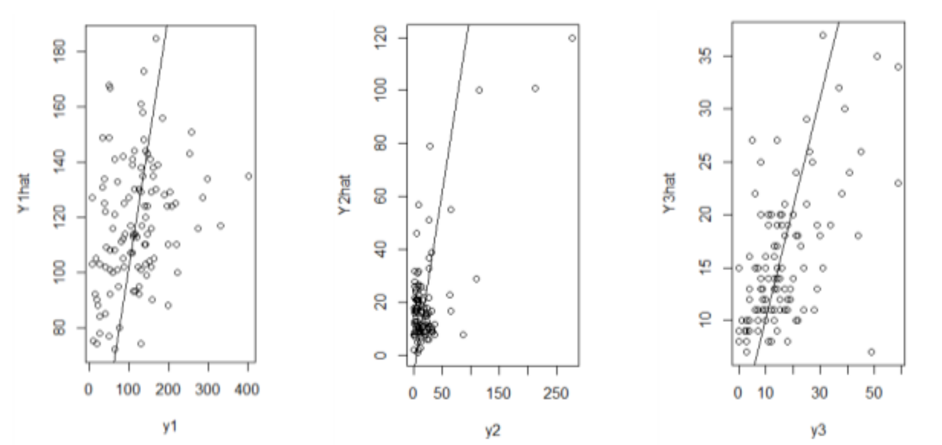
We use the Mean Squared Error (MSE) to measure the difference in the average squared between the estimated and the actual value in order to determine whether the model fits the data well. The Root Mean Squared Error (RMSE) reveals the estimates of standard deviation of each response, where their standard deviation of response observations are reported in Table 1. The MSE and RMSE for the response variables are tabulated in

Table 5. The Mean Squared Error (MSE) and Root Mean Squared Error (RMSE) for each response variable.

	Y1	Y2	Y3
MSE	4821.05	707.31	104.17
RMSE	69.43	26.59	10.21

. It is shown that the RMSE values are close the standard deviation of each response. This empirical results also prove that the predicted responses are relatively very close to the observations values.

In addition to RMSE written in Table 5, the scatter plots of true and prediction values of each response are exhibited in order to show that the MPIGR model is good at predicting the observed data. To support this result, Figure 2 is displayed to see how spread out the residuals are. Based on Figure 2, the fitting values for Y₁ and Y₃ are better than those of Y₂. This empirical results, of course, can be improved. These findings become the big concerns for the next research that are possibly related to the spatial dependencies among the responses that are discussed in the coming section.

4. Discussion

The result of the significant partial test shows that at a significance level α = 0.05, the predictor variables that significantly influence the number of infants, child, and maternal deaths are the percentage of antenatal care visit by pregnant women (X₁), the percentage of pregnant women who received Fe3 tablet (X₂), the percentage of complete neonatal visits (X₃), the percentage of Low Birth Weight (LBW) (X₄), the percentage of healthy house (X₅), the percentage of active integrated service post (X₆), the percentage of infants received vitamin A (X₇), and the percentage of births that are assisted by health workers (X₈).

According to regression coefficient of the MPIGR model, the percentage of Low Birth Weight (LBW) (X₄) gave the greatest effect to the number of infant mortality (Y₁), the number of under-five children mortality (Y₂), and the number of maternal mortality (Y₃). However, it has inappropriate dependencies with Y₁, Y₂, and Y₃. Based on these results, we need to look at the pattern of the relationship between the predictor and the response variables below.

The pattern of the relationship between the predictor and response variables leads to the conclusion that several predictors have an inappropriate relationship structure. The percentage of antenatal care visit by pregnant women (X₁) has a negative relationship with Y₁ and Y₂, while it has positive or inappropriate relationship with Y₃. The percentage of pregnant women who received Fe3 tablet (X₂) has negative dependencies with Y₂, while it has a positive or inappropriate relationship with Y₁ and Y₃. On the other side, the percentage of complete neonatal visits (X₃) has negative or appropriate dependencies with Y₁ and Y₃. Meanwhile, the percentage of Low Birth Weight (LBW) (X₄) has positive dependencies with all of the response variables. However, conflicting results were obtained for all of the response variables.

The percentage of healthy house (X₅) has negative relationship with Y₁ and Y₃, while it has positive or inappropriate sign with Y₂. The percentage of active integrated service post (X₆) has negative dependencies with Y₁ and Y₃, while it has a positive effect on Y_2. The percentage of infants received vitamin A (X₇) has a positive relationship with Y₁ and Y₃, while it has negative or appropriate dependencies with Y₂. The latter one, the percentage of births assisted by health workers (X₈), has negative dependencies with Y₃, while it has an inappropriate relationship with Y₁ and Y₃. This finding means that, even though all predictor variables are statistically significant, not all of them have an appropriate relationship with all of the response variables.

The results of this study lead us to more deeply investigate the appropriate method for modeling the data. We assume that the spatial aspect needs to be added to the modeling. Thus, to support our assumptions, a spatial heterogeneity test was carried out in order to test the differences in the characteristics between one point of observation and another. The test statistics used the Glejser test with the null hypothesis (H₀) is no spatial heterogeneity and the alternative hypothesis (H₁) is that there is spatial heterogeneity. The results of the test is G² =1309.84, which is higher than ${\chi }_{0.05,24}^2=36.415$. Therefore, the decision is to reject H₀, which means that the response variables have a spatial heterogeneity and can be modelled using a spatial model in future work. The local model, for example, geographically weighted regression, for MPIGR will be the big concern for our future research.

5. Conclusions

The Multivariate Poisson Inverse Gaussian Regression (MPIGR) is the development of the Poisson Inverse Gaussian univariate regression (PIGR) model. The MPIGR model that is proposed in this research accommodates the exposure variable within the model, as the quality of each observation unit level, to overcome the overdispersion problem. The parameter estimation is performed using the Maximum Likelihood Estimation (MLE), followed by the Newton–Raphson iteration. Meanwhile, to simultaneously and partially examine the MPIGR model, the Maximum Likelihood Ratio Test (MLRT) method is used.

The empirical results of the application, where the unit of observation is city or municipality, showed that all eight predictors affect the three response variables, i.e., number of infants, under-five children, and maternal mortality in Java, Indonesia. The predictors are the percentage of antenatal care visits of pregnant women, the percentage of pregnant women receiving Fe3 tablets, the percentage of neonatal visits complete, the percentage of low birth weight babies (LBW), the percentage of healthy homes, the percentage of active integrated service post, the percentage of babies receiving vitamin A, and the percentage of deliveries assisted by health workers.

According to computational problems that were suffered by factorial calculation in Bessel function, the factorial simplification in the third modification of Bessel function was done to avoid the large numbers incomputable by a computer. The proposed simplification procedure is very crucial to make the fitting of the MPIGR models computable. The application of the MPIGR model to real data in this study is limited to three-count response variables. Based on the result of the spatial heterogeneity test, the spatial aspects are needed to model the data with the spatial model in future research.

References

- Consul, P.; Famoye, F. Generalized poisson regression model. Commun. Stat. Theory Methods 1992, 21, 89–109. [Google Scholar] [CrossRef]
- Holla, M.S. On a poisson-inverse gaussian distribution. Metr. Int. J. Theor. Appl. Stat. 1967, 11, 115–121. [Google Scholar] [CrossRef]
- Dean, C.; Lawless, J.F.; Willmot, G.E. A mixed poisson-inverse-gaussian regression model. Can. J. Stat. 1989, 17, 171–181. [Google Scholar] [CrossRef]
- Hilbe, J.M. Poisson Inverse Gaussian Regression. In Modeling Count Data; Cambridge University Press (CUP): Cambridge, UK, 2014; pp. 162–171. [Google Scholar]
- Karlis, D.; Xekalaki, E. A Simulation Comparison of Several Procedures for Testing the Poisson Assumption. J. R. Stat. Soc. Ser. D Stat. 2000, 49, 355–382. [Google Scholar] [CrossRef] [Green Version]
- Ouma, V.M. Poisson Inverse Gaussian (PIG) Model for Infectious Disease Count Data. Am. J. Theor. Appl. Stat. 2016, 5, 326. [Google Scholar] [CrossRef] [Green Version]
- Xie, F.-C.; Wei, B.-C. Influence analysis for Poisson inverse Gaussian regression models based on the EM algorithm. Metrika 2007, 67, 49–62. [Google Scholar] [CrossRef]
- Zha, L.; Lord, D.; Zou, Y. The Poisson inverse Gaussian (PIG) generalized linear regression model for analyzing motor vehicle crash data. J. Transp. Saf. Secur. 2014, 8, 18–35. [Google Scholar] [CrossRef] [Green Version]
- Ghitany, M.E.; Karlis, D. An EM Algorithm for Multivariate Mixed Poisson. Appl. Math. Sci. 2012, 6, 6843–6856. [Google Scholar]
- United Nations Inter-agency Group for Child Mortality Estimation (UN IGME). Levels & Trends in Child Mortality: Report 2018, Estimates Developed by the United Nations Inter-Agency Group for Child Mortality Estimation; United Nations Children’s Fund: New York, NY, USA, 2018. [Google Scholar]
- WHO; UNICEF; UNFPA; The World Bank. Maternal Mortality: Level and Trends 2000 to 2017; World Health Organization: Geneva, Switzerland, 2019; ISBN 978-92-4-151648-8. [Google Scholar]
- Moucheraud, C.; Worku, A.; Molla, M.; Finlay, J.E.; Leaning, J.; Yamin, A.E. Consequences of maternal mortality on infant and child survival: A 25-year longitudinal analysis in Butajira Ethiopia (1987–2011). Reprod. Health 2015, 12, S4. [Google Scholar] [CrossRef] [PubMed] [Green Version]
- Miaou, S.P.; Lord, D. Modeling Traffic Crash–Flow Relationships for Intersections Dispersion Parameter, Functional Form, and Bayes Versus Empirical Bayes Methods. Transp. Res. Rec. J. Transp. Res. Board 2003, 1840, 31–40. [Google Scholar] [CrossRef]
- Willmot, G.E. The Poisson-Inverse Gaussian distribution as an alternative to the negative binomial. Scand. Actuar. J. 1987, 1987, 113–127. [Google Scholar] [CrossRef]
- Stein, G.Z.; Juritz, J.M. Bivariate compound poisson distributions. Commun. Stat. Theory Methods 1987, 16, 3591–3607. [Google Scholar] [CrossRef]
- Stein, G.Z.; Zucchini, W.; Juritz, J.M. Parameter estimation for the Sichel distribution and its multivariate extension. J. Am. Stat. Assoc. 1987, 82, 938–944. [Google Scholar] [CrossRef]
Figure 1.
Histogram of response variables.
Figure 2.
The plot of the actual and the estimate values.