Image Analysis Applications for Building Inter-Story Drift Monitoring

Abstract

Structural health monitoring techniques have been applied to several important structures and infrastructure facilities, such as buildings, bridges, and power plants. For buildings, accelerometers are commonly used for monitoring the accelerations induced by ambient vibration to analyze the structural natural frequencies for further system identification and damage detection. However, due to the relatively high cost of the accelerometers and data acquisition systems, accelerometer-based structural health monitoring systems are challenging to deploy in general buildings. This study proposed an image analysis-based building deformation monitoring method that integrates a small single-board computer, computer vision techniques, and a single-camera multiple degree-of-freedom algorithm. In contrast to other vision-based systems that use multiple expensive cameras, this method is designed for a single camera configuration to simplify the installation and maintenance procedures for practical applications. It is designed to monitor the inter-story drifts and torsional responses between the ceiling and floor of a story that is being monitored in a building, aiming to maximize the monitored structural responses. A series of 1:10 reduced scale static and dynamic structural experiments demonstrated that the proposed method and the device prototype are capable of analyzing images and structural responses with an accuracy of 0.07 and 0.3 mm from the results of the static and dynamic experiments, respectively. As digital imaging technology has been developing dramatically, the accuracy and the sampling rates of this method can be improved accordingly with the development of the required hardware, making this method practically feasible for an increasing number of applications for building structural monitoring.

1. Introduction

Structural health monitoring is capable of sensing structural damage by detecting minor variations in structural vibration characteristics or deformation, providing a chance for early warning and the minimization of further damage. The health of structures such as buildings and bridges can be degraded not only by the natural aging of materials, inter-material bonding, and connections but also by over-weighting, natural hazards such as earthquakes, or improper renovations. The degradation of the structure may induce a change in the natural frequencies and vibration modes of the structure or induce slight deformation of the structure. Most of the changes in the vibrational characteristics and deformation of structures are typically not observed by humans, yet they can be detected by the sensing systems used for structural health monitoring, minimizing the risk of severe damage or the collapse of structures.

Structural health monitoring techniques are being developed for monitoring current buildings, bridges, and other civil structures [1,2,3]. Many of the structural health monitoring systems on buildings and bridges use accelerometers not only to identify the structural natural frequencies and vibration modes [4,5,6] but also have been used recently for dynamic response estimation, including displacement and internal forces [7,8]. In addition to accelerometers, different types of sensors or sensing methods, such as film-based strain gauges [9,10], optical fiber sensors [11,12,13], acoustic emission [14,15,16], cameras [17,18,19,20,21,22], or even global navigation satellite systems [2], are being developed and employed for structural health monitoring. A variation in the system stiffness or vibration modal shapes could indicate a certain level of structural damage [6,23,24]. Several studies have investigated improving the accuracy of the identification of damage [25,26], reducing the noise induced by sensors or environmental interference [26], minimizing sensing synchronization errors [27,28,29], and reducing the number of sensors required to capture the necessary vibration modes or failure modes [30].

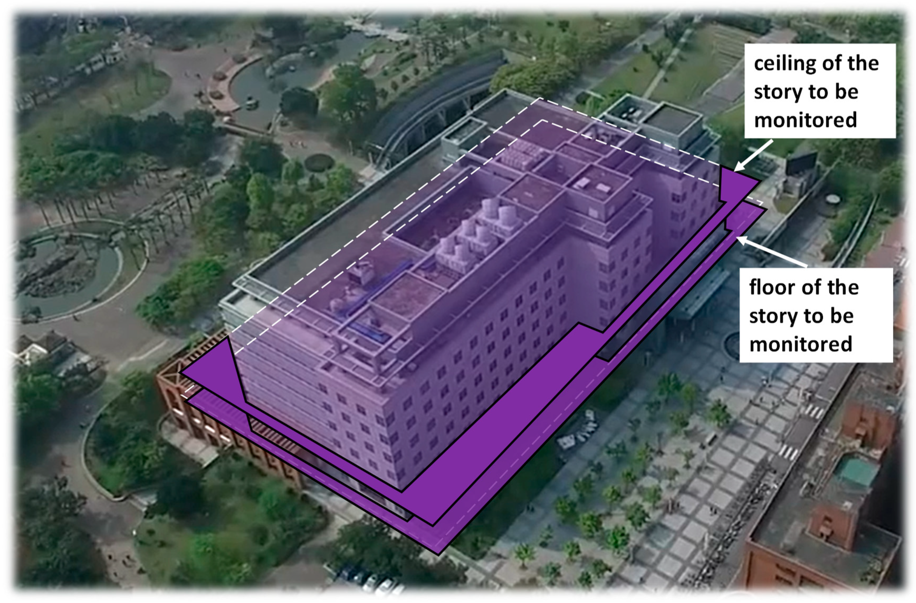
Experience has shown that the collapse of many buildings from earthquakes is initiated by the failure of a weakened story [31,32,33]. Inter-story responses are the movement of the ceiling with respect to the floor, as shown in the colored planes in Figure 1. Large inter-story responses and residual displacement [34,35,36] could indicate large deformation of structural and imply a risk of structural damage or failure [37].

For better and wider applications of structural health monitoring, more sensor options are required, in addition to the ability to monitor different types of failure, with different levels of accuracies and costs, to address practical limitations and requirements. While an accelerometer is good at capturing vibrations, which are relatively high frequency responses, it does not sense slow structural responses such deformation induced by settlement, material creep, or gradual deformations or displacements. While displacement sensors such as linear variable differential transducers (LVDT) are relatively accurate for measuring displacements, they require additional supporting fixtures that are sometimes difficult to install due to limited interior space, limiting their practical applications. Due to the relatively high cost of hardware, even a relatively small number of accelerometers or LDVTs with minimal data acquisition systems could be much higher than the cost many the building owners would like to invest.

As digital imaging technology has been dramatically developing in recent years, several researchers have investigated the use of image analysis for measuring structural deformation and vibration responses [38]. In structural laboratories, image analysis techniques have been developed and employed to measure displacements [29], deformations [39], settlement and shrinkage [40], and cracks [41,42]. Some structural experiments have been performed to measure the uniaxial displacements of structures by analyzing images taken by a single camera [43]. Three-dimensional displacements and accelerometers can be estimated by analyzing images taken by two or more cameras by using stereo triangulation techniques [44]. Strain fields of a plane structural surface can be estimated by tracking a dense mesh of feature points painted on regions of interest [45]. Strain fields of curved surfaces can be calculated by further employing image un-distortion and rectification techniques [42]. Concrete crack development can be observed and measured by using a displacement-to-crack mapping formula [46]. Structural damage can be further quantified by calculating certain damage indices using information obtained from image analysis [47]. Image analysis has potential for use in post-earthquake building safety evaluations by analyzing two or more surveillance cameras using stereo triangulation techniques [44,48]. Some image analysis programs are freely [49] or commercially available in the market, and some of them are specifically designed for structural experiments.

This study proposes a building deformation monitoring method that integrates a small single-board computer, computer vision technique, and a single-camera multiple degree-of-freedom algorithm. Based on the existing computer-vision techniques, the proposed method measures multiple degrees of freedom of the story displacements with consideration of the camera movement. Rather than using a conventional stereo triangulation method, which requires two or more cameras and a sophisticated calibration procedure, this method uses only one camera and is designed to monitor the inter-story drifts and torsional responses between the ceiling and the floor of a story in a building, aiming to simplify the installation and maintenance procedures and to maximize the monitored structural response. The system is capable of analyzing inter-story responses both online and offline. The offline analysis can analyze previous inter-story responses using recorded videos with a sampling rate of the highest imaging frame rate of the camera hardware. The online analysis can instantly monitor the current inter-story responses using a sampling rate that the computer speed can achieve. At the time of this article being written, the hardware cost of the device prototype, including a single-board Raspberry Pi 3B (manufactured by Raspberry Pi Foundation, UK) equipped with a small camera lens, is less than one-hundred US dollars. The proposed method and the device prototype can achieve an offline sampling rate of 30 Hz and an online sampling rate of 3 Hz, with an inter-story drift accuracy of 0.0175% (i.e., the ratio of relative displacement of 0.07 mm to a story height of 400 mm) and 0.075% (i.e., the ratio of 0.3 mm to 400 mm) from static and dynamic experiments, respectively. Since the proposed algorithm does not limit the computational speed and accuracy, the sampling rates and measurement accuracy will continue to increase as digital imaging technology keeps improving.

2. Methods

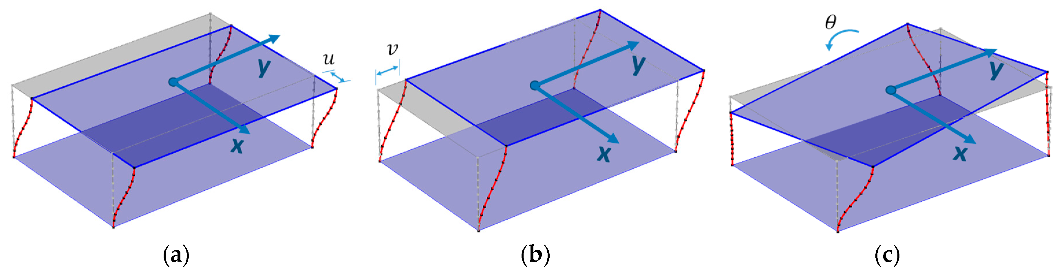
The inter-story responses measured in this work include the inter-story displacements u and v of the ceiling and the torsion θ with respect to the floor. While the columns of a building could deform when they are subjected to lateral forces, it is commonly assumed in structural design that the floors are rigid. For example, for the health monitoring of the first floor, the ground floor and its ceiling, which are transparently colored in Figure 1, are assumed to be rigid diaphragms. In practice, the vertical displacements of columns are relatively small as compared to their lateral displacements as the axial stiffness of a typical column is much larger than its lateral stiffness; therefore, the ceiling and the floor are assumed to be parallel. The proposed method would produce significant errors on inter-story drifts, if the building is collapsed or is partially collapsed, in which the ceiling is not parallel to the floor. Based on the above assumptions, the inter-story responses of each floor are simplified into three degrees of freedom, u, v, and θ, as shown in Figure 2. The displacements plotted in Figure 2 are scaled for demonstration, i.e., typical structural deformations are normally much smaller than they appear in Figure 2.

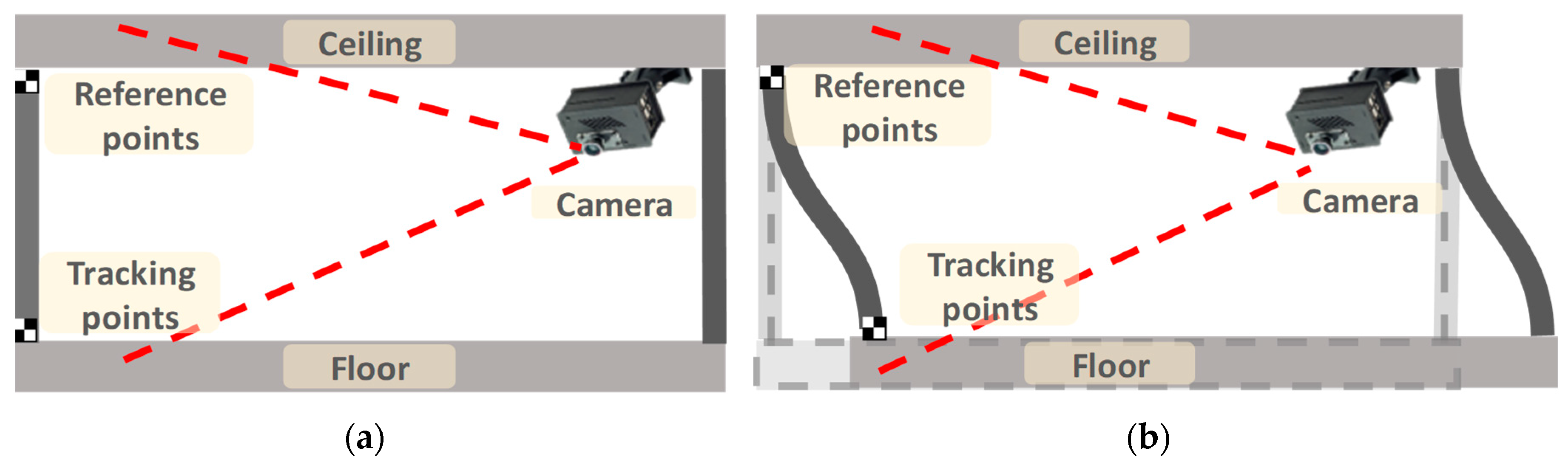
The technical basis for monitoring the inter-story response by a single camera is to monitor the positions of two sets of targets in the images: tracking points and the reference points. It is assumed that the camera is fixed to the ceiling above the story that is being monitored, with the target points referring to objects that are fixed to the floor of the monitored story, and the reference points being objects fixed to the ceiling of the monitored story. When inter-story deformation occurs, the positions of the tracking points in the image taken by the camera change, as shown in Figure 3. By analyzing the movements of the tracking points in the images, the inter-story responses can be estimated. The reference points, which are affixed to the ceiling, are used to estimate the possible unintended movement of the camera. Even a minimal unintended movement of the camera can induce a relatively large change in tracking point and reference point positions in the image. To prevent obtaining incorrect inter-story responses, the movement of the camera needs to be estimated so that a more accurate inter-story response can be obtained.

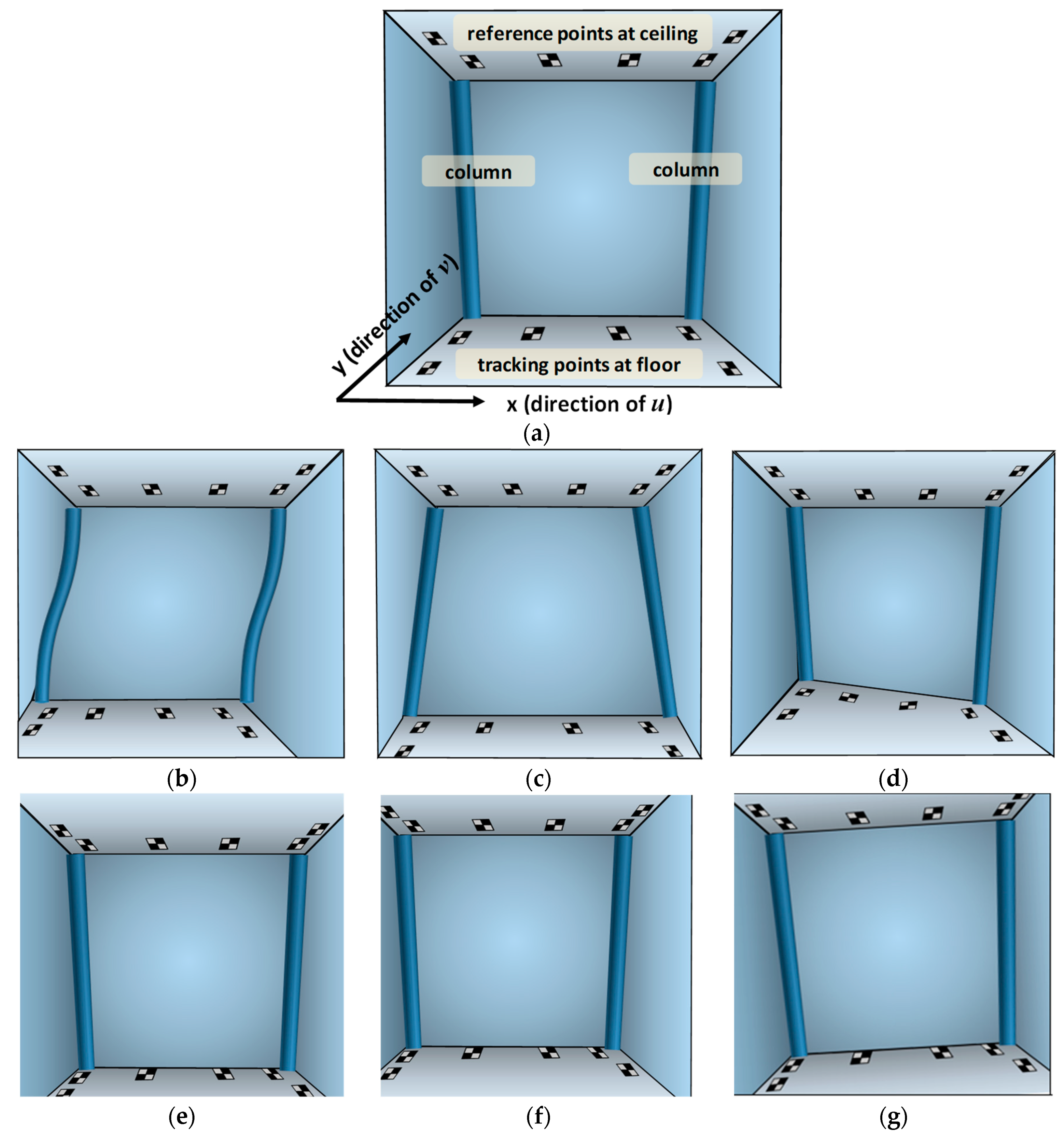
While Figure 3 presents the basic idea of the proposed method in two dimensions, the real world is three-dimensional. Figure 4 demonstrates images taken by a camera installed to align with the ceiling of the monitored story. Figure 4a presents the un-deformed inter-story. The positions of the tracking points and the reference points are continuously tracked by the camera of the single-board computer. Figure 4b–d presents the inter-story responses of u, v, and θ, respectively, images that represent the proposed inter-story motion model. Figure 4e–g presents the model motion of the unintended camera movement, which include the pitch, yaw, and roll, respectively. While the unintended camera movement can theoretically also have translational movements, only three rotational movements are considered here because images are generally much more sensitive to camera rotations than translations. Even a minimum camera rotation can induce significant image movement. Simplification of the camera movement can also simplify the nonlinear simultaneous equations that will be introduced later, easing the convergence of their numerical solution.

An accurate image measurement is based on an accurate camera calibration. The image analysis techniques employed in this work include camera calibration, target tracking, and point projection. Camera calibration is used to estimate the parameters of the camera, including the intrinsic parameters and the extrinsic parameters. The intrinsic parameters include the focal lengths $f_x$ and $f_y$, the principal points $c_x$ and $c_y$, the distortion coefficients $k_1 to k_6$, $p_1$, and $p_2$. The extrinsic parameters include $r_x$, $r_y$,$r_z$, $t_x$, $t_y$, and $t_z$, which represent the geometric relationship between the camera and the global coordinate system. While the global coordinate system can be defined arbitrarily, it must be consistent throughout the entire process. It is suggested that the global coordinate system be aligned to the coordinate system used in the engineering drawing of the structure, so the engineers who will use this system have a consistent coordinate system when using the proposed system. The definition of the global coordinate system is especially important in the installation phase of the monitoring system (see Step 1 and 2 described below).

Target tracking allows the defining of the tracking and reference points in the initial image (where the inter-story is un-deformed) and automatically and precisely determines where these points are in later images taken by the same camera, during which the inter-story may have deformed. Many types of target tracking methods have been developed and are widely employed, such as template matching [50], enhanced correlation correction [51], optical flow [52], feature-based image alignment [53], machine learning based methods [54], and many other variations of these methods. These methods have been thoroughly developed in the C++ open source computer vision library OpenCV [55,56]. As compared to other methods, the optical flow method is relatively fast and gives subpixel precision and is thus employed in this work.

Given the 3D coordinate of an arbitrary point and the camera parameters, the point projection method calculates the theoretical position that this point should appear in the image. The aforementioned image analysis techniques have been well-developed by using OpenCV [55,56], and thus, the programming implementation developed in this study adopts this library. The technical details of this method can be found in many previous studies [55] and are not presented in this study.

This work integrates the inter-story motion model (Figure 4b–d), camera movement model (Figure 4e–g), the aforementioned computer vision techniques, and an iterative process that solves the nonlinear simultaneous equations. The equations relate the inter-story responses, camera movements, camera parameters, image coordinates, and 3D coordinates of the reference and tracking points. The Gauss–Newton algorithm [57,58] is used to iteratively solve the equations and obtain the camera movements and the inter-story responses.

The procedures of the proposed method include the following major steps:

Step 1:

Install a camera with which images can be acquired by a computer. The camera should be fixed at the ceiling of the story to be monitored. In the prototype tests in this work, the camera/computer is a single-board computer (Raspberry Pi 3B) equipped with a camera lens. In future practical applications, the camera/computer device can be a dedicated camera system or a security surveillance system that has been installed in the structure that can be accessed by the designed program to run on the system computer and can access the images acquired by the system cameras. The image resolution in this experiment is set to 640 by 480 pixels, while most of the surveillance cameras nowadays have a higher resolution.

Step 2:

Select two or more targets that can be clearly seen by the camera and are firmly fixed with the ceiling and the floor, separately. Each target should have a highly contrasting pattern, such as text on a sign, a bolt, an intersection of bricks, a cross pattern, or any other target that has border lines along at least two different directions in the image, so that the image analysis can recognize its movement in the image. The targets that are on the ceiling are denoted as reference points, while the remaining targets are the tracking points. Obtain the 3D global coordinates of the reference and the tracking points. The 3D coordinates can be estimated by examining the engineering drawings of the structure or by conventional direct measurements. While this step may have significant labor costs, it only needs to be done once at the installation phase of the system. In this study, we use ${\mathit{X}}_{Ref\left(m\right)}$ and ${\mathit{X}}_{Trk\left(n\right)}^t$ to represent the global coordinates of the mth reference points and the nth tracking points at time t, respectively. The ${\mathit{X}}_{Ref\left(m\right)}$ and ${\mathit{X}}_{Trk\left(n\right)}^t$ are used to calculate their image coordinates, which are further introduced in the Step 7. The time t is zero at Step 2. The global coordinates of the reference points ${\mathit{X}}_{Ref\left(m\right)}$ are supposed to be unchanged during the entire monitoring duration and thus does not need a superscript t.

Step 3:

Obtain the camera parameters $\mathit{C}$ by camera calibration. The camera calibration can be carried out by using the one-step calibration method proposed by the first author [29], where the method estimates the camera parameters by simply using only one photo. The camera parameters $\mathit{C}$ to be obtained in this step include the focal lengths $f_x$ and $f_y$, the principal point $c_x$ and $c_y$, the distortion coefficients $k_1 to k_6$, $p_1$, and $p_2$, and the extrinsic parameters $r_x^t$, $r_y^t$,$r_z^t$, $t_x^t$, $t_y^t$, and $t_z^t$ that represent the geometric relationship between the camera and the global coordinate system, where the superscript t is zero at Step 3. The mathematical meanings of these parameters can be found in many computer vision textbooks [55], and a brief introduction is presented in [29]. While the mathematics of these parameters may seem complicated, the idea is simple: Once we have these parameters, we know the geometry of how any arbitrary 3D object in the global coordinate system would be projected onto the image through this camera. The software implementation of the camera calibration is also included in the software prototyped in this work. By giving the image coordinates and the 3D coordinates of the reference and tracking points, the camera parameters are obtained by using the camera calibration technique [59]. In the prototyped software, the initial image that represents the initial un-deformed status is also obtained in this step. In this study, we use ${\mathit{I}}_{Ref\left(m\right)}^t$ and ${\mathit{I}}_{Trk\left(n\right)}^t$ to represent the image coordinates of the mth reference points and the nth tracking points at time t, respectively.

Step 4:

Acquire the current image. By using the point tracking technique, the image coordinates of each reference point ${\mathit{I}}_{Ref\left(m\right)}^t$ and tracking points ${\mathit{I}}_{Trk\left(n\right)}^t$ are obtained. In this work, the optical flow algorithm as implemented in OpenCV [60] is used to track the points.

Step 5:

Guess the inter-story response and the camera movement. In general, the analyzed inter-story response and camera movement of the previous time step is taken as the initial guess. If it is the first time step of the analysis, the inter-story response and the camera movement are guessed as zeros. ${\mathit{U}}^t$ is used to represent the guessed inter-story response at time t, which is a 3-by-1 matrix ${\langle u^t v^t {\theta }^t\rangle }^{\mathrm{T}}$, and ${\mathit{C}}_R^t$ is used to represent the guessed camera movement, which is a 3-by-1 matrix ${\langle r_{pitch}^t r_{yaw}^t r_{roll}^t\rangle }^{\mathrm{T}}$. The superscript T represents matrix transpose. This study uses a 1-by-6 matrix ${\mathit{d}}^t$ to represent the combination of ${\mathit{U}}^t$ and ${\mathit{C}}_R^t$, as shown in the following Equation. ${\mathit{d}}^t$ is adjusted in Step 10.

$${\mathit{d}}^t= \langle {\mathit{U}}^t|{\mathit{C}}_R^t\rangle =\langle u^t v^t {\theta }^t r_{pitch}^t r_{yaw}^t r_{roll}^t\rangle$$

(1)

Step 6:

Calculate the 3D coordinates of each of the tracking points ${\mathit{X}}_{Trk\left(n\right)}^t$ according to the guessed inter-story response ${\mathit{U}}^t$ using the inter-story model. The following equation is used to calculate the 3D coordinates of these points, where ${\mathit{X}}_c$ is the torsional center of the monitored story, which can be obtained from the modal analysis result of the structural analysis. If the structural analysis is not available, the torsional center can be replaced with the centroid of the monitored story. The inter-story drift of a point induced by its inter-story torsion is at the order of the torsion (in unit of radian) times the distance between the point and the torsional center. Since the quantity of inter-story torsion is typically small (i.e., normally much smaller than a thousandth radians), an inaccurately setting of torsional center, if that is about a few millimeters inaccurate, only induces a relatively small errors of displacements.

$${\mathit{X}}_{Trk\left(m\right)}^t=\left(\left(\begin{array}{ccc}cos{\theta }^t& -sin{\theta }^t& 0\\ sin{\theta }^t& cos{\theta }^t& 0\\ 0& 0& 1\end{array}\right)\left({\mathit{X}}_{Trk\left(m\right)}^0-{\mathit{X}}_c\right)\right)+{\mathit{X}}_c +\left(\begin{array}{c}{u}^t\\ v^t\\ 0\end{array}\right).$$

(2)

Step 7:

Calculate the extrinsic parameters $r_x^t$, $r_y^t$,$r_z^t$, $t_x^t$, $t_y^t$, and $t_z^t$ at time t according to the unintended camera movement. The unintended camera movement changes the geometric relationship between the camera and the global coordinate; therefore, the extrinsic parameters $r_x^t$, $r_y^t$,$r_z^t$, $t_x^t$, $t_y^t$, and $t_z^t$ must be updated by

$${\langle r_x^t r_y^t r_z^t\rangle }^T = \mathit{Rodrigues}\left({\mathit{R}}_3^t\right)$$

(3)

where ${\mathit{R}}_3^t$, $t_x^t$, $t_y^t$, and $t_z^t$ are obtained from.

$$\left(\begin{array}{cc}\left(\begin{array}{ccc}& & \\ & {\mathit{R}}_3^t& \\ & & \end{array}\right)& \begin{array}{c}{t}_x^t\\ t_y^t\\ t_z^t\end{array}\\ \begin{array}{ccc}0& 0& 0\end{array}& 1\end{array}\right) = {\left({\left(\begin{array}{cc}Rodrigues\left(\begin{array}{c}{r}_x\\ r_y\\ r_z\end{array}\right)& \begin{array}{c}{t}_x\\ t_y\\ t_z\end{array}\\ \begin{array}{ccc}0& 0& 0\end{array}& 1\end{array}\right)}^{-1}\left(\begin{array}{cc}Rodrigues\left(\begin{array}{c}{r}_{pitch}^t\\ r_{yaw}^t\\ r_{roll}^t\end{array}\right)& \begin{array}{c}0\\ 0\\ 0\end{array}\\ \begin{array}{ccc}0& 0& 0\end{array}& 1\end{array}\right)\right)}^{-1}$$

(4)

and the Rodrigues function converts a 3-by-1 rotation vector to a 3-by-3 rotation matrix and can also convert a 3-by-3 rotation matrix back to a 3-by-1 rotational vector. While a 3-by-3 rotation matrix is widely used in 3D coordinate transformation, the 3-by-1 rotation vector is the most compact form to represent a rotation as any rotation matrix has just three degrees of freedom (i.e., $r_{pitch}^t$, $r_{yaw}^t$, and $r_{roll}^t$). The mathematical formulation of the Rodrigues function can be found in computer vision textbooks (e.g., [55]) and is not repeated here. The OpenCV library also provides a C++ implementation of the Rodrigues function, which is employed in this work. The idea behind the above mathematical formulation is simple: Since the camera is slightly rotated, the geometric relationship between the camera and the global coordinate is changed, and thus the extrinsic parameters $r_x^t$, $r_y^t$,$r_z^t$, $t_x^t$, $t_y^t$, and $t_z^t$ of the camera must be adjusted. ${\mathit{C}}^t$ is used to represent the adjusted camera parameters, which is the same as $\mathit{C}$ where the extrinsic parameters are replaced with $r_x^t$, $r_y^t$,$r_z^t$, $t_x^t$, $t_y^t$, and $t_z^t$. The superscripts t indicate that the orientation of the camera can vary over time.

Step 8:

Obtain the projected (calculated) image coordinates of each reference ${\widehat{\mathit{I}}}_{Ref\left(m\right)}^t$ and tracking point ${\widehat{\mathit{I}}}_{Trk\left(m\right)}^t$ by using the point projection technique. The projected image coordinates are the calculated image coordinates of these points. The point projection can be carried out by the following Equations:

$${\widehat{\mathit{I}}}_{Ref\left(m\right)}^t=PointProjection\left({\mathit{C}}^t, {\mathit{X}}_{Ref\left(m\right)}\right),$$

(5)

$${\widehat{\mathit{I}}}_{Trk\left(n\right)}^t=PointProjection\left({\mathit{C}}^t,{\mathit{X}}_{Trk\left(n\right)}^t\right).$$

(6)

The function $PointProjection$ is detailed in previous literature (e.g., [55]) and is not repeated here. $PointProjection$ calculates the image coordinate $\widehat{\mathit{I}}$ with which an arbitrary 3D point $\mathit{X}$ should project on an image according to the camera parameters. OpenCV provides a C++ implementation, whose function is named projectPoints, to carry out the point projection, which is used in this work.

In general, the calculation of (5) and (6) can be expressed by the following procedures, where ${\mathit{C}}^t$ consists of the current camera parameters $f_x$, $f_y$, $c_x$, $c_y$, $k_1 to k_6$, $p_1$, $p_2$, $r_x^t$, $r_y^t$,$r_z^t$, $t_x^t$, $t_z^t$, and $t_z^t$. $\mathit{X}$ is expressed as ${\langle x_W y_W z_W\rangle }^{\mathrm{T}}$, and $\widehat{\mathit{I}}$ is expressed as ${\langle x_i y_i\rangle }^{\mathrm{T}}$.

$$\left(\begin{array}{c}\begin{array}{c}{x}_c\\ y_c\\ z_c\end{array}\\ 1\end{array}\right)=\left(\begin{array}{cc}Rodrigues\left(\begin{array}{c}{r}_x^t\\ r_y^t\\ r_z^t\end{array}\right)& \begin{array}{c}{t}_x^t\\ t_y^t\\ t_z^t\end{array}\\ \begin{array}{ccc}0& 0& 0\end{array}& 1\end{array}\right)\left(\begin{array}{c}\begin{array}{c}{x}_w\\ y_w\\ z_w\end{array}\\ 1\end{array}\right),$$

(7)

$$\left(\begin{array}{c}{x}_n\\ y_n\end{array}\right)=\left(\begin{array}{c}{x}_c\\ y_c\end{array}\right)/z_c,$$

(8)

$$k=\frac{1+k_1\left(x_n^2+y_n^2\right)+k_2{\left(x_n^2+y_n^2\right)}^2+k_3{\left(x_n^2+y_n^2\right)}^3}{1+k_4\left(x_n^2+y_n^2\right)+k_5{\left(x_n^2+y_n^2\right)}^2+k_6{\left(x_n^2+y_n^2\right)}^3}$$

(9)

$$\left(\begin{array}{c}{x}_{\mathit{d}}\\ y_{\mathit{d}}\end{array}\right)=\left(\begin{array}{cc}k+2p_1{y}_n+3p_2{x}_n& p_2{y}_n\\ p_1{x}_n& k+2p_2{x}_n+3p_1{y}_n\end{array}\right)\left(\begin{array}{c}{x}_n\\ y_n\end{array}\right),$$

(10)

and

$$\left(\begin{array}{c}{x}_i\\ y_i\\ 1\end{array}\right)=\left(\begin{array}{ccc}{f}_x& 0& c_x\\ 0& f_y& c_y\\ 0& 0& 1\end{array}\right)\left(\begin{array}{c}{x}_{\mathit{d}}\\ y_{\mathit{d}}\\ 1\end{array}\right)$$

(11)

Step 9:

Compare the projected image coordinates and the actual image coordinates. Calculate the vector of errors $\mathit{e}$, which represents the difference between the projected coordinates and the actual coordinates of all reference points and tracking points. The vector $\mathit{e}$ is a 1-by-(2M + 2N) vector where M and N represent the number of reference points and tracking points, respectively.

$${\mathit{e}}^t=\langle \left({\widehat{\mathit{I}}}_{Ref\left(m\right)}^t-{\mathit{I}}_{Ref\left(m\right)}^t\right)|\left({\widehat{\mathit{I}}}_{Trk\left(n\right)}^t-{\mathit{I}}_{Trk\left(n\right)}^t\right)\rangle$$

(12)

Step 10:

Adjust the guessed inter-story responses and the camera movement ${\mathit{d}}^t$ according to the error vector ${\mathit{e}}^t$. In this work, the adjustment is based on the Gauss–Newton algorithm [57,58]. We define a function $f$ to integrate the calculations from Step 4 to 9:

$${\mathit{e}}^t= f\left({\mathit{d}}^t\right)$$

(13)

A Jacobian matrix $\mathit{J}$ can be calculated. The Jacobian matrix is obtained by applying a finite difference calculation, where the associated calculation procedures can be obtained in many numerical analysis textbooks (e.g., [57,58]) and is not repeated here. The solution of $∆{\mathit{d}}^t$ (i.e., the story responses and camera movements) would have a unique solution if there more than three targets on both of the ceiling and the floor, and the targets are not on a straight line. If so, every story displacement and camera movement would have a unique appearance on the camera, making the Jacobian matrix nonsingular, and theoretically there would be a unique solution.

$$j_{ij}=\frac{\partial e_i}{\partial d_j},$$

(14)

where $j_{ij}$ is the element of the ith row and the jth column of matrix $\mathit{J}$, $e_i$ is the ith element of vector ${\mathit{e}}_{}^t$, and $d_j$ is the jth element of vector ${\mathit{d}}^t$. The adjustment of ${\mathit{d}}^t$ is given as

$$∆{\mathit{d}}^t= {\left(-{\left({\mathit{J}}^T\mathit{J}\right)}^{-1}{\mathit{J}}^T{\mathit{e}}^t\right)}^{\mathrm{T}}$$

(15)

${\mathit{d}}^t$ is then replaced with ${\mathit{d}}^t+∆{\mathit{d}}^t$.

Step 11:

If the adjustment $∆{\mathit{d}}^t$ is sufficiently close to a zero vector, such as which norm is below a small number like 10⁻⁶, go to the next step. Otherwise, go to Step 6 for the next iteration.

Step 12:

Output the data by writing to files, plotting to graphs, and displaying on the screen. The data include the inter-story responses, camera movement, and many detailed data aforementioned. The inter-story responses can be further used for structural safety early warning; however, this is not in the scope of this paper.

Step 13:

Go to Step 4 until we stop the monitoring.

3. Verification by Reduced Scale Experiments

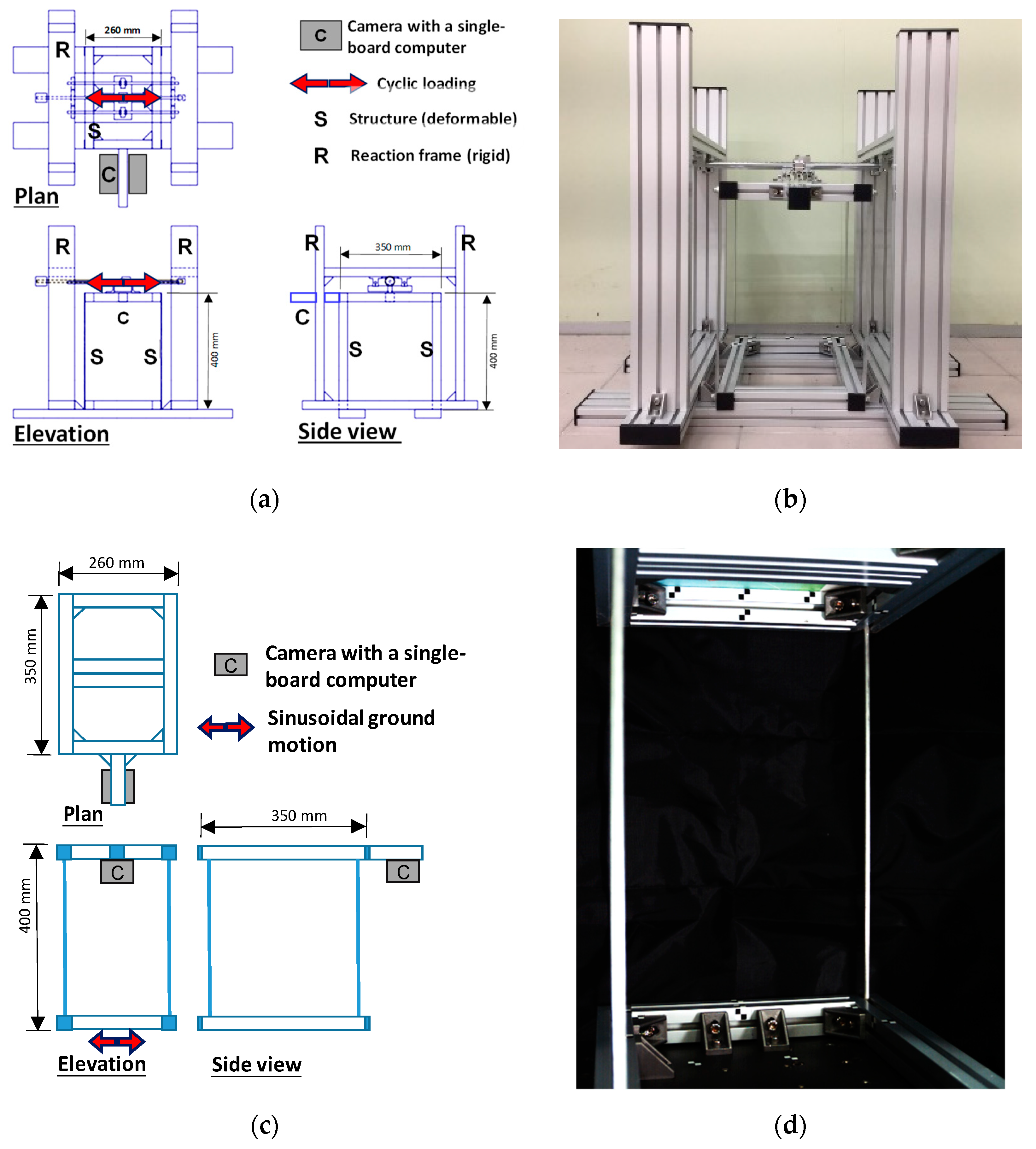
The proposed method to estimate the inter-story responses was verified by a set of reduced scale experiments. Considering the high cost of a full-scale structural test and the infeasibility of deforming a real building, the verification was performed by carrying out a series of one-tenth scaled structural experiments. Two sets of experiments were carried out: static and dynamic experiments. The static experiments are used to investigate the accuracy of the proposed method for slow deformations, where the applications of the proposed system are for monitoring the residual deformation and slow deformation induced by creep, subsidence, or slow responses. The dynamic experiments are used to represent the dynamic inter-story responses induced by earthquakes. The dimensions of the specimens and the accessories are displayed in the structural design plots shown in Figure 5. The camera resolution was set to 640 by 480 pixels, not higher than most of the surveillance cameras nowadays. Figure 5d displays the overall specimen, which was taken by another camera.

In the static experiments, a cyclic uniaxial displacement history was applied at the top of the specimen along the u direction through an accurately controlled step motor and a screw bar. In the dynamic experiments, the reduced scale building specimen was placed on a shaker table providing a ±3-mm amplitude sinusoidal uniaxial table motion, equivalent to an inter-story drift ratio of ±0.75%. Two tests were performed: one with 1-Hz of table motion applied and the other with 3-Hz of applied table motion. Both table motions were only applied for the first three seconds, allowing the specimen to gradually obtain a free vibration after the table motion. While the table motion is uniaxial, the building specimen responses include all of the inter-story degrees of freedom including the bilateral displacements u, and v, and the torsion θ due to a certain level of structural eccentricity. The eccentricity could be induced by the asymmetry of the building geometry or the structural design. In the experiment, the eccentricity was mainly induced by the additional frame for camera installation. Camera rotation induced by the vibration is also possible and is considered in the analysis procedure of the proposed method. Considering the multiaxial responses of the specimen, we employ a high precision optical system equipped with relatively expensive industrial-level high speed image analysis system [61], as it is relatively complicated to measure dynamic multiaxial responses by conventional devices such as LVDTs.

4. Results

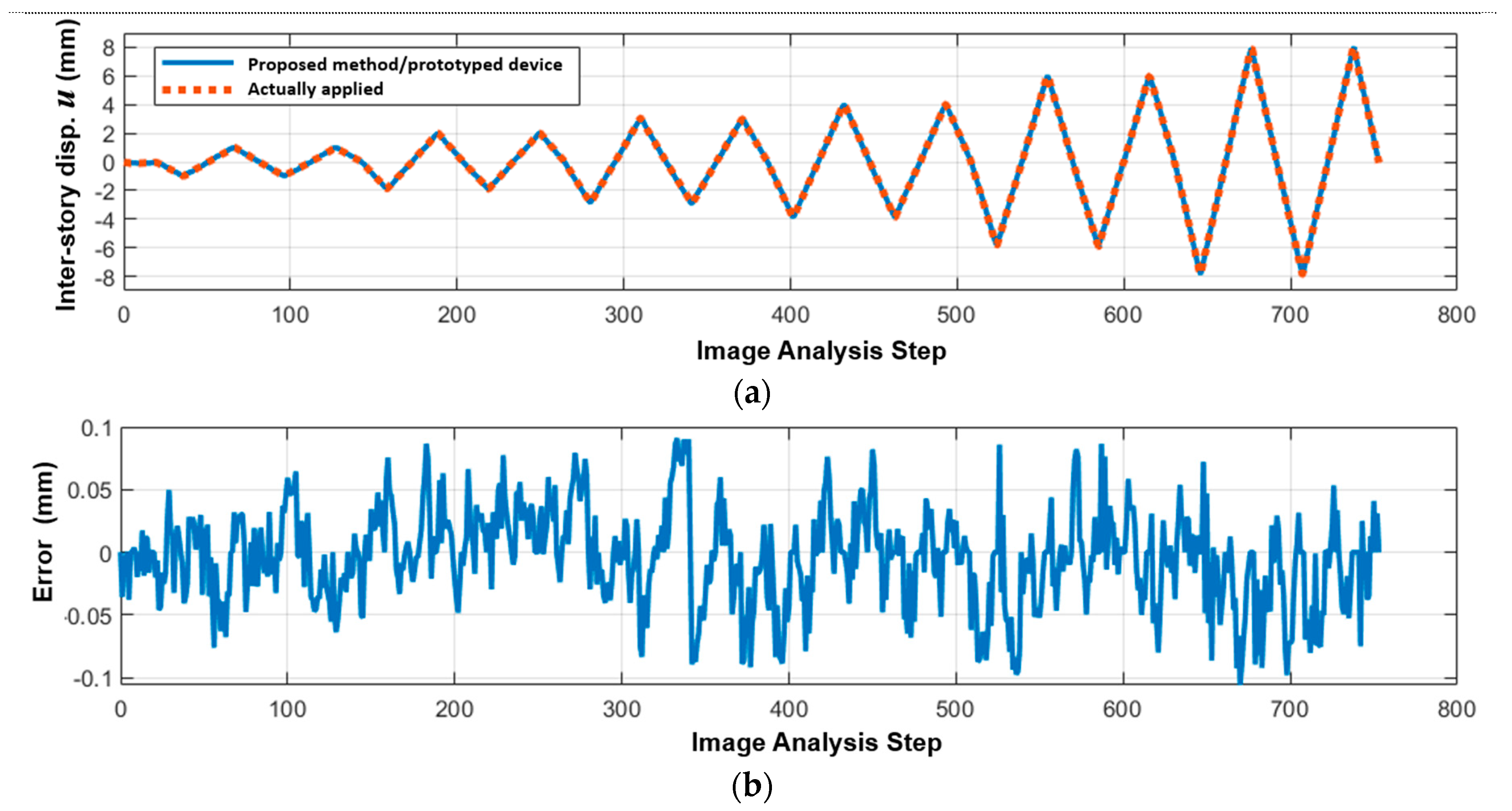
A comparison of the actual applied inter-story drift and the measured inter-story u is shown in Figure 6. The errors between the actual applied and measured inter-story responses u at the peaks are generally smaller than 0.1 mm. The maximum 0.1 mm error is equivalent to 0.1 pixels of positioning error in image point tracking and is equivalent to a 0.025% inter-story drift ratio, or a 1-mm accuracy if the specimen is scaled to full scale, which is relatively small. While this accuracy is not comparable to conventional displacement devices such as an LVDT, which normally achieves an accuracy of 0.05 mm, the accuracy of the proposed method is capable of measuring significant inter-story responses in practical applications.

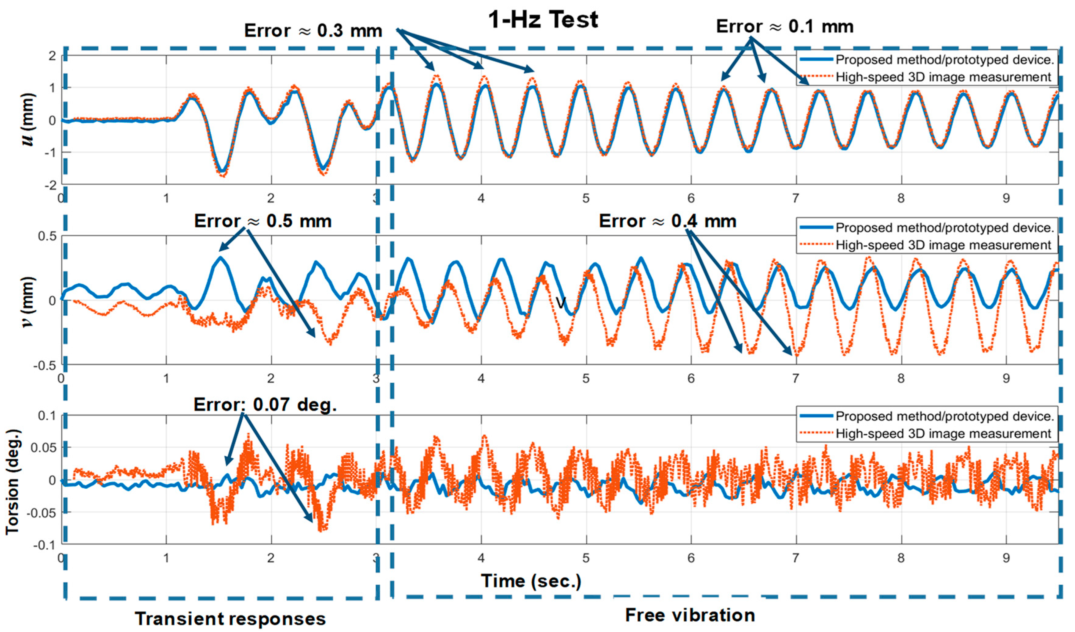
The measured responses are shown in Figure 7 for the 1-Hz test, where the inter-story responses are relatively small. The displacement of u is ±1.8 mm, while the displacement of v is ±0.4 mm, and the torsion is even smaller at ±0.08 degrees. Comparing the differences between the responses measured by the proposed method/prototyped device and the industrial 3D image measurement, the maximum displacement errors along u and v observed in these tests are within ±0.3 mm and ±0.5 mm, respectively. The error along u gradually reduced to 0.1 mm during the later period of the steady state response. The displacement v resulted in larger errors than u mainly because it is along the depth direction of the camera, which is the direction that a typical camera has little sensitivity. If the error along the depth direction does not meet the requirement, more than one camera could be considered. The description is added in the revised manuscript.

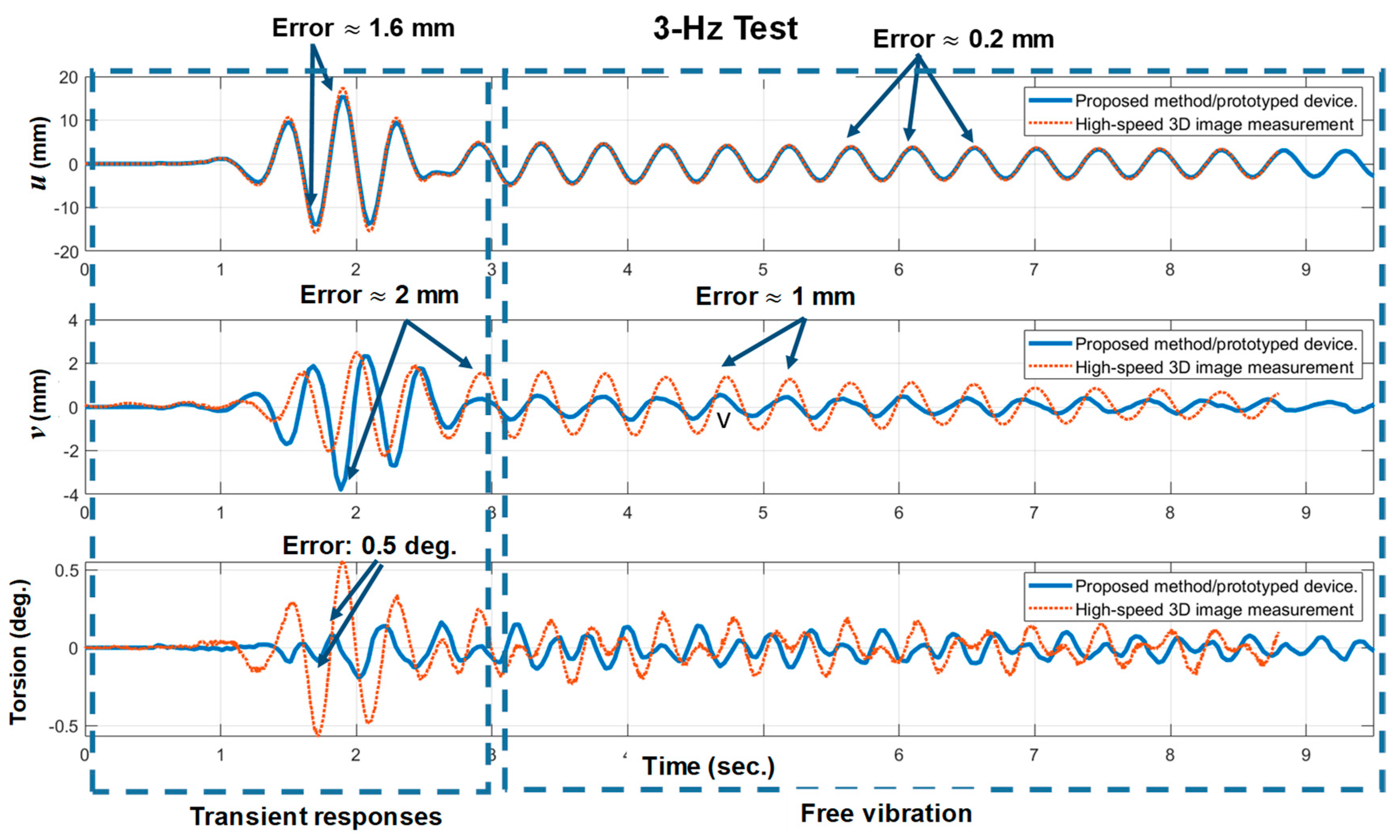
In the 3-Hz test (Figure 8), the inter-story responses are almost ten times larger than those in the 1-Hz test, mainly because the excitation is closer to the natural frequency of the specimen (i.e., 2.2 Hz). The observed natural frequencies generally matched its numerical modal analysis. Along the u-direction, the inter-story drifts reached maximum amplitudes of 4.32% (i.e., the ratio of 17.3 mm to 400 mm) and −3.93% (i.e., the ratio of −15.7 mm to 400 mm) in the transient state (from 0 to 3 s), and gradually remained at a 4.5-mm amplitude in the steady state (after 4 s). The differences between the responses measured by the proposed method/prototyped device and the industrial 3D image measurement are up to 0.5% (i.e., the ratio of 2 mm to 400 mm) at major peaks in transient responses and approximately 0.13% (i.e., the ratio of 0.5 mm to 400 mm) during the steady state response. Along the v-direction, in addition to an error larger than 0.5% (i.e., the ratio of 2 mm to 400 mm), a phase difference is also observed.

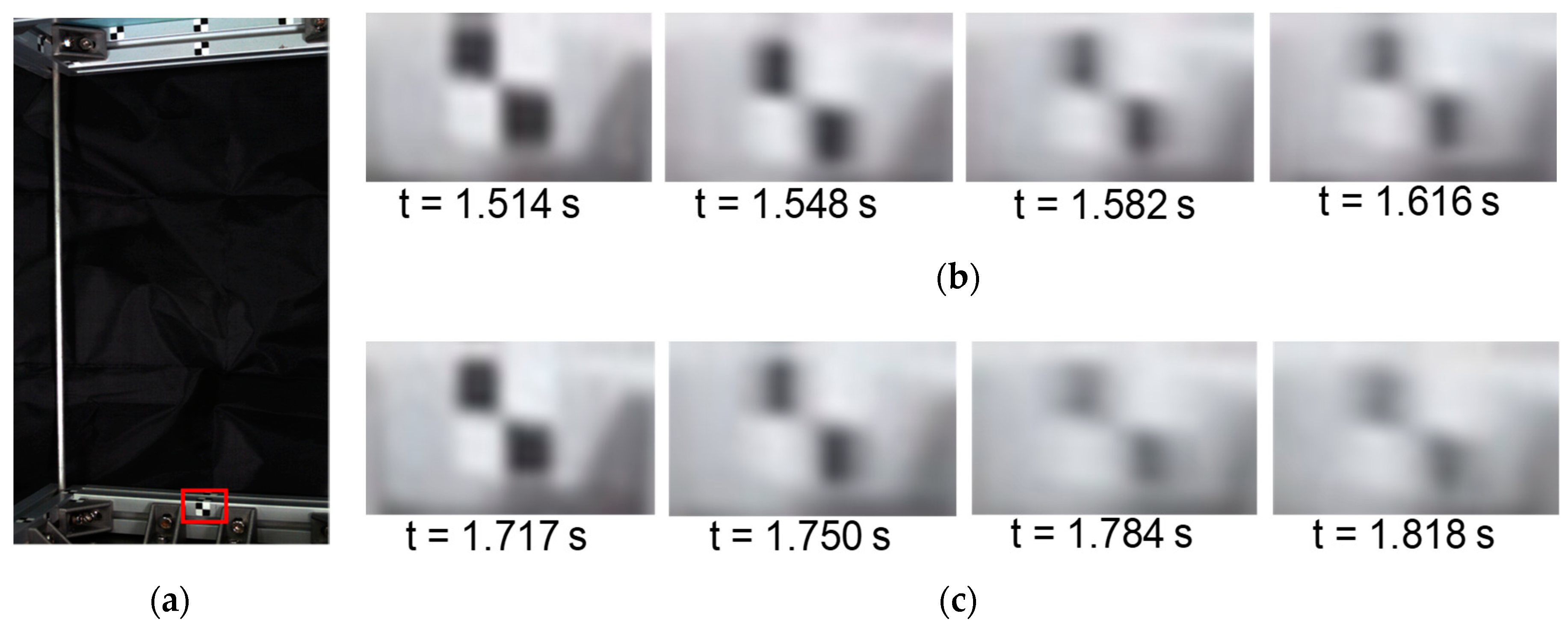
In both tests, image blurs can be observed in the photos taken by the prototyped device due to the rapid movement of the tracking points. The image blurs are especially significant in the 3-Hz test when the relative velocities of the tracking points are high. Figure 9 shows example images of one of the tracking points on the lower floor (indicated by a red box in Figure 9a). The images shown in Figure 9b,c are a sub-region of the photos. At time t = 1.514 s when the relative displacement u just went through a peak, the tracking point is clearly visible in the photo. Within only three image frames (approximately 0.1 s), the image became significantly blurred (Figure 9b). The image became clear again at the negative peak, yet when going back to positive from negative, the images once again became blurred. While Figure 9 shows two relatively severe cases, the image blurring occurred in almost every cycle of motion during the transient responses. While the point tracking technique is now typically capable of positioning a target in image with an accuracy as small as 0.02 to 0.03 pixels in crystal clear images (references), image blur would significantly reduce the accuracy. Reducing the exposure time of the camera could reduce image blur to improve the point tracking accuracy. Using strong environmental lights or adopting a camera with high low-light sensitivity can help reduce the exposure time of the camera, and thus further reduce the blur due to fast movement.

The rolling shutter effect is one of the potential sources of the measurement error. Typically, an image taken by a camera with a rolling shutter is generated by scanning a scene line by line from the top to the bottom of the image, rather than being taken at a single instant in time. A camera with a global shutter, which conceptually generates an image at an instant in time, is typically expensive. Most of the inexpensive cameras in the consumer market are rolling shutter based. In our cases, the reference points at the upper part of the image are scanned earlier than the tracking points at the lower part. The time differences between these points generate errors in the inter-story response measurement. Unfortunately, reducing exposure time by using a stronger environmental lighting does not improve the rolling shutter effect. The image blurring effect and many other site dependent effects could be significantly higher than those in the laboratory. It also implies that higher camera resolution does not guarantee similar accuracy.

5. Conclusions

This work developed an image-based inter-story response measurement method and developed a small device prototype with a camera and a single-board computer, aiming to provide a cost-effective measurement method for structural health monitoring. With the aid of modern computer vision techniques, the developed method includes an inter-story motion model, a camera movement model, and an iterative procedure that estimates the inter-story responses. Instead of adopting triangulation that requires accurate time synchronization and a complicated calibration process, this method requires only a single camera installed at either the ceiling above or the floor below the target story for monitoring and is capable of capturing three degrees of freedom of the inter-story responses. Considering that images are sensitive to any slight camera rotation, this method estimates the camera rotations by monitoring reference points located at the same floor that the camera is fixed at.

A series of experiments were performed to verify the developed method. A one-tenth reduced scale one-bay portal frame specimen was constructed and used for the experiments. In the static experiment that deformed the specimen through a cyclic uniaxial inter-story drift history up to 2% (i.e., the ratio of 8 mm to 400 mm), this method captured the drift with a maximum error of 0.025% (i.e., 0.1 mm). Two dynamic experiments were carried out that gave sinusoidal motions of 1-Hz and 3-Hz, respectively, at the bottom of the specimen. In the 1-Hz experiment, the inter-story responses were within ±0.45% (i.e., ±1.8 mm), and the measurement errors were approximately 0.075% (i.e., the ±0.3 mm) over the transient response, gradually reducing to 0.025% (i.e., of 0.1 mm) during free vibration. In the 3-Hz experiments where the inter-story responses were up to 4.5% (i.e., 18 mm), the maximum measurement during the transient response was 0.5% (i.e., 2 mm), reducing to 0.1% (i.e., 0.4 mm) during the free vibration. The presence of image blurring induced by the rapid motion of tracking points was discussed, possibly resulting in significant measurement error. Technical issues induced by these effects should be seriously addressed. In addition, a realistic ground motion, which has sophisticated frequency contents, could also induce complicated imaging effects. It requires further study with improved analytical consideration and more realistic experiments to further improve the accuracy of the image analysis method. The rolling shutter effect was also discussed as possibly contributing to errors in the measurement. While this method using a low-cost device does not aim to replace conventional structural health monitoring, it provides fairly satisfactory accuracy for many practical applications in engineering, especially considering rapid developments in hardware performance and the resolution of digital cameras and imaging technology.

References

- Song, G.; Wang, C.; Wang, B. Structural Health Monitoring (SHM) in Civil Structures. Appl. Sci. 2017, 7, 789. [Google Scholar] [CrossRef]
- Kumbert, T.; Schneid, S.; Reindl, L. A Wireless Sensor Network Using GNSS Receivers for a Short-Term Assessment of the Modal Properties of the Neckartal Bridge. Appl. Sci. 2017, 7, 626. [Google Scholar] [CrossRef] [Green Version]
- Shokravi, H.; Shokravi, H.; Bakhary, N.; Rahimian Koloor, S.S.; Petrů, M. A Comparative Study of the Data-Driven Stochastic Subspace Methods for Health Monitoring of Structures: A Bridge Case Study. Appl. Sci. 2020, 10, 3132. [Google Scholar] [CrossRef]
- Dackermann, U.; Yu, Y.; Niederleithinger, E.; Li, J.; Wiggenhauser, H. Condition Assessment of Foundation Piles and Utility Poles Based on Guided Wave Propagation Using a Network of Tactile Transducers and Support Vector Machines. Sensors 2017, 17, 2938. [Google Scholar] [CrossRef] [PubMed] [Green Version]
- Zhu, L.; Fu, Y.; Chow, R.; Spencer, B.F.; Park, J.W.; Mechitov, K. Development of a High-Sensitivity Wireless Accelerometer for Structural Health Monitoring. Sensors 2018, 18, 262. [Google Scholar] [CrossRef] [PubMed]
- Udatha, L.; Pasupuleti, V.D.K.; Rajaram, B. Structural Health Monitoring from Human-Induced Vibrations Using Accelerometer Sensors. Emerg. Trends Civ. Eng. 2020, 61, 57–67. [Google Scholar]
- Roohi, M.; Erazo, K.; Rosowsky, D.; Hernandez, E.M. An Extended Model-Based Observer for State Estimation in Nonlinear Hysteretic Structural Systems. Mech. Syst. Signal Process. 2020, 146, 107015. [Google Scholar] [CrossRef]
- Roohi, M.; Hernandez, E.M. Performance-based Post-Earthquake Decision Making for Instrumented Buildings. J. Civ. Struct. Health Monit. 2020, 10, 775–792. [Google Scholar] [CrossRef]
- Lee, B.M.; Loh, K.J. Carbon Nanotube Thin Film Strain Sensors: Comparison Between Experimental Tests and Numerical Simulations. Nanotechnology 2019, 30, 439502. [Google Scholar] [CrossRef] [Green Version]
- Tiedemann, R.; Lepke, D.; Fischer, M.; Pille, C.; Busse, M.; Lang, W. A Combined Thin Film/Thick Film Approach to Realize an Aluminum-Based Strain Gauge Sensor for Integration in Aluminum Castings. Sensors 2020, 20, 3579. [Google Scholar] [CrossRef]
- Antunes, P.; Lima, H.; Varum, H.; André, P. Optical Fiber Sensors for Static and Dynamic Health Monitoring of Civil Engineering Infrastructures: Abode Wall Case Study. Measurement 2012, 45, 1695–1705. [Google Scholar] [CrossRef]
- Ye, X.-W.; Su, Y.-H.; Xi, P.-S. Statistical Analysis of Stress Signals from Bridge Monitoring by FBG System. Sensors 2018, 18, 491. [Google Scholar]
- Her, S.-C.; Chung, S.-C. Dynamic Responses Measured by Optical Fiber Sensor for Structural Health Monitoring. Appl. Sci. 2019, 9, 2956. [Google Scholar] [CrossRef] [Green Version]
- Ono, K. Structural Health Monitoring of Large Structures Using Acoustic Emission–Case Histories. Appl. Sci. 2019, 9, 4602. [Google Scholar] [CrossRef] [Green Version]
- Lugovtsova, Y.; Bulling, J.; Boller, C.; Prager, J. Analysis of Guided Wave Propagation in a Multi-Layered Structure in View of Structural Health Monitoring. Appl. Sci. 2019, 9, 4600. [Google Scholar] [CrossRef] [Green Version]
- Jin, H.; Yan, J.; Li, W.; Qing, X. Monitoring of Fatigue Crack Propagation by Damage Index of Ultrasonic Guided Waves Calculated by Various Acoustic Features. Appl. Sci. 2019, 9, 4254. [Google Scholar] [CrossRef] [Green Version]
- Cheng, C.; Kawaguchi, K. A Preliminary Study on the Response of Steel Structures Using Surveillance Camera Image with Vision-Based Method During the Great East Japan Earthquake. Measurement 2015, 62, 142–148. [Google Scholar] [CrossRef]
- Feng, D.; Feng, M.Q. Experimental Validation of Cost-Effective Vision-Based Structural Health Monitoring. Mech. Syst. Signal Process. 2017, 88, 199–211. [Google Scholar] [CrossRef]
- Harvey, P.S., Jr.; Elisha, G. Vision-based Vibration Monitoring Using Existing Cameras Installed within a Building. Struct. Control Health Monit. 2018, 25, e2235. [Google Scholar] [CrossRef]
- Yu, L.; Tian, Y.; Wu, W. A Dark Target Detection Method Based on the Adjacency Effect: A Case Study on Crack Detection. Sensors 2019, 19, 2829. [Google Scholar] [CrossRef] [Green Version]
- Fradelos, Y.; Thalla, O.; Biliani, I.; Stiros, S. Study of Lateral Displacements and the Natural Frequency of a Pedestrian Bridge Using Low-Cost Cameras. Sensors 2020, 20, 3217. [Google Scholar] [CrossRef] [PubMed]
- Deng, G.; Zhou, Z.; Shao, S.; Chu, X.; Jian, C. A Novel Dense Full-Field Displacement Monitoring Method Based on Image Sequences and Optical Flow Algorithm. Appl. Sci. 2020, 10, 2118. [Google Scholar] [CrossRef] [Green Version]
- Zeng, L.; Xiao, Y.; Chen, Y.; Jin, S.; Xie, W.; Li, X. Seismic Damage Evaluation of Concrete-Encased Steel Frame-Reinforced Concrete Core Tube Buildings Based on Dynamic Characteristics. Appl. Sci. 2017, 7, 314. [Google Scholar] [CrossRef]
- He, L.; Reynders, E.; García-Palacios, J.H.; Carlo Marano, G.; Briseghella, B.; De Roeck, G. Wireless-Based Identification and Model Updating of a Skewed Highway Bridge for Structural Health Monitoring. Appl. Sci. 2020, 10, 2347. [Google Scholar] [CrossRef] [Green Version]
- Karayannis, C.G.; Chalioris, C.E.; Angeli, G.M.; Papadopoulos, N.A.; Favvata, M.J.; Providakis, C.P. Experimental Damage Evaluation of Reinforced Concrete Steel Bars Using Piezoelectric Sensors. Constr. Build. Mater. 2016, 105, 227–244. [Google Scholar] [CrossRef]
- Teng, Z.; Teng, S.; Zhang, J.; Chen, G.; Cui, F. Structural Damage Detection Based on Real-Time Vibration Signal and Convolutional Neural Network. Appl. Sci. 2020, 10, 4720. [Google Scholar] [CrossRef]
- Veluthedath Shajihan, S.A.; Chow, R.; Mechitov, K.; Fu, Y.; Hoang, T.; Spencer, B.F., Jr. Development of Synchronized High-Sensitivity Wireless Accelerometer for Structural Health Monitoring. Sensors 2020, 20, 4169. [Google Scholar] [CrossRef]
- Bezas, K.; Komianos, V.; Koufoudakis, G.; Tsoumanis, G.; Kabassi, K.; Oikonomou, K. Structural Health Monitoring in Historical Buildings: A Network Approach. Heritage 2020, 3, 796–818. [Google Scholar] [CrossRef]
- Yang, Y.S. Measurement of Dynamic Responses from Large Structural Tests by Analyzing NonSynchronized Videos. Sensors 2019, 19, 3520. [Google Scholar] [CrossRef] [Green Version]
- García, D.; Tcherniak, D. An Experimental Study on the Data-Driven Structural Health Monitoring of Large Wind Turbine Blades using a Single Accelerometer and Actuator. Mech. Syst. Signal Process. 2019, 127, 102–119. [Google Scholar] [CrossRef] [Green Version]
- Park, Y.; Ang, A.H.; Wen, Y.K. Seismic Damage Analysis of Reinforced Concrete Buildings. J. Struct. Eng. 1985, 111, 740–757. [Google Scholar] [CrossRef]
- van de Lindt, J.W.; Bahmani, P.; Mochizuki, G.; Pryor, S.E.; Gershfeld, M.; Tian, J.; Symans, M.D.; Rammer, D. Experimental Seismic Behavior of a Full-Scale Four-Story Soft-Story Wood-Frame Building with Retrofits. II: Shake Table Test Results. J. Struct. Eng. 2016, 142, E4014004. [Google Scholar] [CrossRef]
- Pan, Y.; Ventura, C.E.; Liam Finn, W.D. Effects of Ground Motion Duration on the Seismic Performance and Collapse Rate of Light-Frame Wood Houses . J. Struct. Eng. 2018, 144, 4018112. [Google Scholar] [CrossRef]
- Yazgan, U.; Dazio, A. Post-Earthquake Damage Assessment Using Residual Displacements. Earthq. Eng. Struct. Dyn. 2012, 41, 1257–1276. [Google Scholar] [CrossRef]
- Skolnik, D.A.; Wallace, J.W. Critical Assessment of Interstory Drift Measurements. J. Struct. Eng. 2010, 136, 1574–1584. [Google Scholar] [CrossRef]
- Roohi, M.; Hernandez, E.M.; Rosowsky, D. Nonlinear Seismic Response Reconstruction and Performance Assessment of Instrumented Wood-Frame Buildings—Validation using NEESWood Capstone Full-Scale Tests. Struct. Control Health Monit. 2019, 26, e2373. [Google Scholar] [CrossRef]
- Japan Building Disaster Prevention Association. Standard for Seismic Evaluation of Existing Reinforced Concrete Buildings; Japanese Edition of 2001, English Version 1st; Japan Building Disaster Prevention Association: Tokyo, Japan, 2001. [Google Scholar]
- Ye, X.W.; Dong, C.Z.; Liu, T. A Review of Machine Vision-Based Structural Health Monitoring: Methodologies and Applications. J. Sens. 2016, 2016, 7103039. [Google Scholar] [CrossRef] [Green Version]
- Castillo, E.D.R.; Allen, T.; Henry, R.; Griffith, M.; Ingham, J. Digital Image Correlation (DIC) for Measurement of Strains and Displacements in Coarse, Low Volume-Fraction FRP Composites Used in Civil Infrastructure. Compos. Struct. 2019, 212, 43–57. [Google Scholar] [CrossRef]
- Dzaye, E.D.; Tsangouri, E.; Spiessens, K.; De Schutter, G.; Aggelis, D.G. Digital Image Correlation (DIC) on Fresh Cement Mortar to Quantify Settlement and Shrinkage. Arch. Civ. Mech. Eng. 2019, 19, 205–214. [Google Scholar] [CrossRef]
- Cho, H.-W.; Yoon, H.-J.; Yoon, J.-C. Analysis of Crack Image Recognition Characteristics in Concrete Structures Depending on the Illumination and Image Acquisition Distance through Outdoor Experiments. Sensors 2016, 16, 1646. [Google Scholar] [CrossRef] [Green Version]
- Yang, Y.S.; Yang, C.M.; Huang, C.W. Thin Crack Observation in a Reinforced Concrete Bridge Pier Test using Image Processing and Analysis. Adv. Eng. Softw. 2015, 83, 99–108. [Google Scholar] [CrossRef]
- Yang, Y.S.; Yang, H.C.; Yang, C.M.; Chang, C.H. Dynamic Measurement of an Embankment Dam Shake Table Experiment Using Online Image Analysis. In Proceedings of the International Conference on Computing in Civil and Building Engineering, Tampere, Finland, 5–7 June 2018. [Google Scholar]
- Hsu, D.Y.; Pham, Q.V.; Chao, W.C.; Yang, Y.S. Post-earthquake Building Safety Evaluation using Consumer-grade Surveillance Cameras. Smart Struct. Syst. 2020, 25, 531–541. [Google Scholar]
- Yang, Y.S.; Huang, C.W.; Wu, C.L. A Simple Image-based Strain Measurement Method for Measuring the Strain Fields in an RC-Wall Experiment. Earthq. Eng. Struct. Dyn. 2012, 41, 1–17. [Google Scholar] [CrossRef]
- Yang, Y.S.; Wu, C.L.; Hsu, T.T.; Yang, H.C.; Lu, H.J.; Chang, C.C. Image Analysis Method for Crack Distribution and Width Estimation for Reinforced Concrete Structures. Autom. Constr. 2018, 91, 120–132. [Google Scholar] [CrossRef]
- Yang, Y.S.; Chang, C.H.; Wu, C.L. Damage Indexing Method for Shear Critical Tubular Reinforced Concrete Structures based on Crack Image Analysis. Sensors 2019, 19, 4304. [Google Scholar] [CrossRef] [Green Version]
- Schumacher, T.; Shariati, A. Monitoring of Structures and Mechanical Systems Using Virtual Visual Sensors for Video Analysis: Fundamental Concept and Proof of Feasibility. Sensors 2013, 13, 16551–16564. [Google Scholar] [CrossRef]
- Yang, Y.S. ImPro Stereo. Official Website of ImPro Stereo, 2020. Available online: https://sites.google.com/site/improstereoen/ (accessed on 1 January 2020).
- Chang, C.; Ma, C. Increasing the Computational Efficient of Digital Cross Correlation by a Vectorization Method. Mech. Syst. Signal Process. 2018, 92, 293–314. [Google Scholar] [CrossRef]
- Evangelidis, G.D.; Psarakis, E.Z. Parametric Image Alignment using Enhanced Correlation Coefficient Maximization. IEEE PAMI 2008, 30, 1858–1865. [Google Scholar] [CrossRef] [Green Version]
- Lucas, B.; Kanade, T. An Iterative Image Registration Technique with an Application to Stereo Vision. In Proceedings of the 7th International Joint Conference on Artificial Intelligence, Vancouver, BC, Canada, 24–28 August 1981; pp. 674–679. [Google Scholar]
- Lowe, D.G. Distinctive Image Features from Scale-Invariant Keypoints. Int. J. Comput. Vis. 2004, 60, 91–110. [Google Scholar] [CrossRef]
- Babenko, B.; Yang, M.H.; Belongie, S. Visual Tracking with Online Multiple Instance Learning. In Computer Vision and Pattern Recognition. In Proceedings of the 2009 IEEE Conference on Computer Vision and Pattern Recognition, Miami, FL, USA, 20–25 June 2009; pp. 983–990. [Google Scholar]
- Kaehler, A.; Bradski, G. Learning OpenCV3: Computer Vision in C++ with the OpenCV Library; O’Reilly Media: Sebastopol, CA, USA, 2016. [Google Scholar]
- OpenCV Team. OpenCV. Available online: https://opencv.org/ (accessed on 1 January 2020).
- Chapra, S.C.; Canale, R.P. Numerical Methods for Engineers, 6th ed.; McGraw Hill: Singapore, 2010. [Google Scholar]
- Burden, R.L.; Faires, J.D. Numerical Analysis, 9th ed.; Cengage Learning: Boston, MA, USA, 2010; ISBN 978-0538733519. [Google Scholar]
- Zhang, Z. A Flexible New Technique for Camera Calibration. IEEE PAMI 2000, 22, 1330–1334. [Google Scholar] [CrossRef] [Green Version]
- Bouguet, J.Y. Pyramidal Implementation of the Lucas Kanade Feature Tracker; Microprocessor Research Labs, Intel Corporation: Santa Clara, CA, USA, 2000. [Google Scholar]
- Basler, A.G. Basler Ace ACA2040-180km Area Scan Camera. Available online: https://www.baslerweb.com/en/products/cameras/area-scan-cameras/ace/aca2040-180km/ (accessed on 1 January 2020).
Figure 1.
The ceiling and floor of a certain story of a building.
Figure 2.
The three degrees of freedom of inter-story responses. (a) Inter-story displacement . (b) Inter-story displacement . (c) Inter-story torsion .
Figure 3.
A 2D inter-story response monitoring using a single camera. (a) Without inter-story displacement. (b) With inter-story displacement.
Figure 4.
Demonstration of images taken by a camera that represent different inter-story responses and camera movement. (a) Un-deformed inter-story. (b) Response to u. (c) Response to v. (d) Response to torsion . (e) Camera pitch. (f) Camera yaw. (g) Camera roll.
Figure 5.
Structural specimens for the reduced scale static and dynamic experiments. (a) Design of the static experiments. (b) Actual configuration of the static experiments. (c) Design of the dynamic experiments. (d) Actual configuration of the dynamic experiments.
Figure 6.
Comparison of the actual applied and measured inter-story displacements and the errors. (a) Measured and actually applied (controlled) inter-story displacement u. (b) Error of measured inter-story displacement u (image measured).
Figure 7.
Inter-story responses for the 1-Hz test.
Figure 8.
Inter-story responses for the 3-Hz test.
Figure 9.
Blurring of images due to movement. (a) Tracking point. (b) Tracking point images blurring due to movement (t = 1.514 to 1.616 s). (c) Tracking point images blurring due to movement (t = 1.717 to 1.818 s).
Publisher’s Note: MDPI stays neutral with regard to jurisdictional claims in published maps and institutional affiliations. |
© 2020 by the authors. Licensee MDPI, Basel, Switzerland. This article is an open access article distributed under the terms and conditions of the Creative Commons Attribution (CC BY) license (http://creativecommons.org/licenses/by/4.0/).
Share and Cite
MDPI and ACS Style
Yang, Y.-S.; Xue, Q.; Chen, P.-Y.; Weng, J.-H.; Li, C.-H.; Liu, C.-C.; Chen, J.-S.; Chen, C.-T. Image Analysis Applications for Building Inter-Story Drift Monitoring. Appl. Sci. 2020, 10, 7304. https://doi.org/10.3390/app10207304
AMA Style
Yang Y-S, Xue Q, Chen P-Y, Weng J-H, Li C-H, Liu C-C, Chen J-S, Chen C-T. Image Analysis Applications for Building Inter-Story Drift Monitoring. Applied Sciences. 2020; 10(20):7304. https://doi.org/10.3390/app10207304
Chicago/Turabian StyleYang, Yuan-Sen, Qiang Xue, Pin-Yao Chen, Jian-Huang Weng, Chi-Hang Li, Chien-Chun Liu, Jing-Syu Chen, and Chao-Tsun Chen. 2020. "Image Analysis Applications for Building Inter-Story Drift Monitoring" Applied Sciences 10, no. 20: 7304. https://doi.org/10.3390/app10207304
Note that from the first issue of 2016, this journal uses article numbers instead of page numbers. See further details here.