High Accuracy Modeling for Solar PV Power Generation Using Noble BD-LSTM-Based Neural Networks with EMA

Abstract

More accurate self-forecasting not only provides a better-integrated solution for electricity grids but also reduces the cost of operation of the entire power system. To predict solar photovoltaic (PV) power generation (SPVG) for a specific hour, this paper proposes the combination of a two-step neural network bi directional long short-term memory (BD-LSTM) model with an artificial neural network (ANN) model using exponential moving average (EMA) preprocessing. In this study, four types of historical input data are used: hourly PV generation for one week (168 h) ahead, hourly horizontal radiation, hourly ambient temperature, and hourly device (surface) temperature, downloaded from the Korea Open Data Portal. The first strategy is employed using the LSTM prediction model, which forecasts the SPVG of the desired time through the data from the previous week, which is preprocessed to smooth the dynamic SPVG using the EMA approach. The SPVG was predicted using the LSTM model according to the trend of the previous time-series data. However, slight errors still occur because the weather condition of the time is not reflected at the desired time. Therefore, we proposed a second strategy of an ANN model for more accurate estimation to compensate for this slight error using the four inputs predicted by the LSTM model. As a result, the LSTM prediction model with the ANN estimation model using EMA preprocessing exhibited higher accuracy in performance than other options for SPVG.

1. Introduction

A report from the International Energy Agency (IEA) revealed that solar, wind, and hydropower energy is growing at a fast rate. In the Renewables 2018 forecast, the market analysis and forecasts from 2019 to 2024 by the IEA [1], the segment of renewables satisfying global energy demand is expected to grow by one-fifth in the following five years to reach 12.4% in 2023. South Korea is one of the most developed countries in Asia, and it is the eighth largest electricity consumer in the world [2]. South Korea has been making a great effort to increase the renewable energy portion of their energy mix [3]. The country has a strong solar photovoltaic (PV) manufacturing industry and supportive policies to achieve the national renewable energy target of 20% by 2030. Moreover, South Korea has revised its nuclear power policy to cut its reliance on nuclear power to facilitate the solar PV adoption manifold.

Solar PVs can be described as the process of converting light (photons) to electricity (voltage), which is called the photovoltaic effect [4]. Due to the decreasing costs of solar PVs, strong government policies, and private partnerships, various incentive schemes for the use of solar PV power generation (SPVG) have been driving the solar power market at an exponential rate in South Korea [5]. However, when connecting to the grid of a solar PV system, the generation, transmission, maintenance, and consumption and the influences of various uncertainty factors, which include sunshine, cloud cover, temperature, module behavior, and relative humidity, are considered [6]. To maintain the security and economic integration of solar PVs in the microgrid, an accurate estimation or prediction of the SPVG plays a key role in enhancing the influence of the PV power on the grid, which improves the reliability of the PV generation capacity of the power plant and the penetration level of the PV system [7,8]. Thus, short-term PV forecasting is a challenge for researchers due to the randomness, volatility, and intermittence of SPVG [9].

There are commonly two types of solar PV forecasting: the direct and indirect methods. The indirect approach is to forecast environmental parameters related to solar PV, such as solar irradiation, wind speed, ambient temperature, device temperature, and other meteorological factors [9,10,11]. Then, the active power output (kilowatts) is calculated from a mathematical prediction model that uses the environmental parameters. However, several problems occur in the accuracy of the prediction of solar PV generation using the indirect method. This approach may not address the application in the field regarding power and energy system engineering and does not consider other factors that affect PV generation, such as the panel-tracking direction or the shadow effect of trees or buildings on each PV system [9,10]. The other approach is a method to predict PV power output directly using historical PV power output data as input variables [11].

In view of the time frame, a solar PV forecast can be classified on a time horizon as ultra-short term (from a few minutes to less than one hour), short term (one hour to several hours ahead), medium term (several hours to one week ahead), and long term (one week to a year or more ahead) [7,12]. In the paper, we used ultra-short-term solar PV forecasting based on the direct approach.

2. Review of Recent Works for SPVG Forecasting

Recently, various SPVG prediction models have been developed on a much-better-integrated solution for the electricity grid, as introduced in [10]. Solar PV forecasting methods can be classified into three approaches [13]: (1) physical, (2) statistical, and (3) artificial intelligence models. The physical approach is a traditional technique that has been generally measured from meteorological and geological data through numerical weather prediction [14], satellite remote sensing measurement [15], and ground measurement devices [16].

However, these techniques require a large number of data samples [17,18,19,20,21] and fitting results, which are sensitive to pathological [22,23] factors and rely on many different types of data [18,19,20,21]. The statistical and machine learning approaches are based on data-driven methods that use historical data, such as solar PV power, irradiation, humidity, and atmospheric temperature, to build the prediction model [6]. The key factor of this statistical approach is minimizing the error of future PV power output by extracting high-quality historical samples [24]. However, these data usually contain irregular errors due to the unrefined input data. Furthermore, heavy preprocessing is required, which results in complexity and cost issues [25] such as requiring an advanced sensor for accurate input data [26], and not be describing a relationship between input features and PV power output although it is relatively clear and simple [27,28].

Machine learning is a subset of artificial intelligence (AI) that consists of techniques that enable computers to make estimations from the data and deliver AI applications [29]. Furthermore, machine learning is a popular forecasting method for time-series data, which is classified as supervised or unsupervised. The machine learning algorithm for solar PV forecasting has generally been a supervised learning algorithm, such as k-nearest neighbors [30], multiple linear regression [31,32], support vector machine [33,34,35], decision tree [36,37], and random forest regression [38]. However, the machine learning approach also requires a large dataset that forecasts SPVG accurately [7].

With the rapid development of the deep learning structures algorithm, the deep neural network (DNN) is an emerging area of machine learning research that has become one of the most popular fields in academia and industry [27]. Deep learning algorithms in each layer create an artificial neural network (ANN) and can learn and make intelligent decisions by themselves. The existing short-term solar PV forecasting technique overcomes traditional machine learning problems, which include slow learning speed, falling into local extrema, gradient disappearance, and lack of a time correlation [9]. However, the deep learning approach uses an ANN that is more layered than machine learning to analyze the accuracy of the data and find patterns [12]. To use these characteristics, several authors have tried to apply deep learning for the accuracy of solar PV power forecasting, such as feed-forward neural networks, convolutional neural networks (CNNs), recurrent neural networks (RNNs), long short-term memory (LSTM), gated recurrent units (GRUs), restricted Boltzmann machines, deep belief networks, and autoencoders, as shown in

Table 1. Comparison of recent work for deep neural networks applied in solar photovoltaic power forecasting.

Author	Year	Forecast Horizon	Error Evaluation Method	Model/Model Type	Description
Liu et al.	2015	24 h ahead	MAPE, MALPE	ANN + Aerosol Index/preprocessing	Liu et al. [10] studied ANNs with the Aerosol Index, which is a measure of how much the wavelength depends on backscattered ultraviolet radiation from the atmosphere because solar PV generation has a strong relationship with the status of solar irradiation from the atmosphere.
Zhu et al.	2016	5 days ahead	RMSE, MAE, MAPE	ANN + wavelet decomposition/preprocessing	Zhu et al. [39] addressed the nonlinear characteristics of ANNs due to nonstationary characteristics of solar PV generation using wavelet decomposition, which separates useful information from a disturbance.
Al-Dahidi et al.	2019	24 h ahead	RMSE, MAE, WMAE	Ensemble	Al-Dahidi et al. [40] proposed an ensemble approach based on the ANN model with an optimization technique to quantize the uncertainty range of the hidden layer of an ANN prediction.
Sun et al.	2018	15 min ahead	MSE/RMSE	CNN	Sun et al. [41] developed the input parameter and several filters of the SUNSET model, which benefits the correlation between SPVG and the contemporaneous images.
Huang et al.	2019	24 h ahead	MAE/RMSE	CNN	Huang et al. [12] introduced PVPNet, which is used for a one-dimensional convolutional layer with anStochastic Gradient Descent (SGD) parameter optimizer for more accurate performance of the short-term solar PV power forecasting approach.
Dohyun et al.	2018	24 h ahead	MSE	CNN + prepredicted value	Dohyun [42] used a convolutional neural network to overcome the limits of the proposed ensemble LSTM/RNN method by removing the long-term dependency of PV data, which applies to predicted weather values.
Li et al.	2019	30 min ahead	MAE, RMSE, MAPE	RNN	In [16], the RNN revealed higher accuracy for short-term solar PV power forecasting compared to traditional machine learning techniques such as SVM, RBF, BPNN, and LSTM.
Wang et al.	2019	One week ahead	MAE, RMSE, MAPE, SDE, PSDE, PRMSE	Hybrid CNN + LSTM	Wang et al. [13] studied the hybrid LSTM–convolutional network, which was evaluated by the technique that considers temporal–spatial feature extraction in two steps. The LSTM model is used to extract the temporal feature information of the historical data, whereas the convolutional neural network extracts the spatial feature information of the historical data.
Chai et al.	2019	A year ahead	MAPE, QRPE, MBE, RMSE, MSE	LSTM + adaptive hyperparameter adjustment	Chai et al. [9] proposed an ultra-short-term PV power forecasting, which reduces the problem of hyperparameters in LSTM using the adaptive hyperparameter adjustment–LSTM model framework.
Zhou et al.	2019	7.5, 15, 30, and 60 min ahead	RMSE/MAE	LSTM + attention mechanism	Zhou et al. [6] employed two LSTM network layers for temperature and solar PV power, which comprise an ensemble deep learning network, adopting an attention mechanism.
Gao et al.	2019	24 h ahead	RMSE/MAD	LSTM + NWP	Gao et al. [11] studied an LSTM for the large-scale solar PV forecasting technique, which preprocesses classifications between ideal weather data and nonideal weather data based on a discrete gray model.
Wang et al.	2018	24 h ahead	MAE/RMSE	Gated recurrent unit (GRU) + K means cluster + Pearson coefficient	Wang et al. [27] proposed two preprocessing methods based on GRU modeling: the Pearson coefficient extracts the main features that affect solar PV power and then examines the relationship between the input data and future PV power output. Then, the K-means method is used as a cluster analysis, which divides each group based on a similar pattern of input data.
Sodsong et al.	2019	24 h ahead	NRMSE	Multiple GRU frames	Sodsong et al. [43] introduced multiple GRU frameworks, which consist of three networks with a single GRU in each network. By splitting the data into multiple smaller networks compared to the normal GRU, this results in shorter training time.
Neo et al.	2017	Two days ahead	MSE	Deep belief network	Neo et al. [44] introduced a deep belief network training algorithm to determine the optimum number of input variables for two-day solar PV forecasting.

. To deal with the nonlinear and periodic problems of SPVG, the traditional method did not guarantee the precision of the forecasting results. According to the above literature, to improve prediction accuracy, as shown in Table 1, most researchers used one of three types of forecasting models, classified as hybrid/ensemble, optimized parameters of DNN, and DNN with preprocessing.

3. Methodology Description

3.1. Exponential Moving Average

An exponential moving average (EMA) is a type of moving average (MA) that emphasizes the most recent data points (i.e., it is a type of weighted MA where more weight is given to the latest data points as the weight exponentially decreases for older data points) [45]. The EMA is also called the exponential weighted moving average (EWMA) or the exponential smoothing method [7].

The EMA model can be described using the following equation [45]:

$${\widehat{E} }_{t+1}= E_t\cdot K+\left(1-K\right)\cdot {\widehat{E} }_t$$

(1)

where the weighted multiplier K is given by K = 2/(N + 1), with N as the period of the EMA calculation. Moreover, $E_t$ is the SPVG at the current time, ${\widehat{E} }_t$ is the estimated EMA of the SPVG at a previous time, and ${\widehat{E} }_{t+1}$ is the future value of the estimated SPVG.

The EWMA [46] is a concept that expands the formula of EMA when more weighting factors exist through the repeated application of the formula using different times. It is expressed using the following equation [46]:

$$\begin{array}{c}{\widehat{E} }_t= K·[P{V}_t +(1-K)·P{V}_{t-1}+{(1-K)}^{2 }·P{V}_{t-2} + \cdots + {(1-K)}^{\phi }·P{V}_{t-\phi }]+\\ {\left(1-K\right)}^{\phi +1}·{\widehat{E} }_{t-\left(\phi +1\right)}\end{array}$$

(2)

for any suitable $\phi \in \left(0,1,2,\dots ,n\right).$

3.2. Long Short-Term Modeling

Neural networks are a set of algorithms that artificially imitate biological neurons, which are the basis for human cognition functions. An RNN is a type of neural network where the output from the previous step is the input to the current step. The RNN can generate a sequence of data so that each sample data point can be assumed to be dependent on the previous sequences. If RNNs can accomplish the sample data, they would be extremely useful. However, as a sequence of data increases the gap between the input and reference data, it is difficult for RNNs to keep past data in memory due to the vanishing gradient problem, which decreases in long-term dependencies and eventually disappears.

The LSTM model or architecture extends the memory of RNNs. It was introduced by Hochreiter and Schmidhuber in 1997. This model mitigates the vanishing gradient problem, which is caused by the repeated application of the recurrent weight matrix in the RNN. In the LSTM model, the recurrent weight matrix is not only replaced by the identity function in the carousel, but it is also controlled by a few noble gates.

3.2.1. Structure of the LSTM

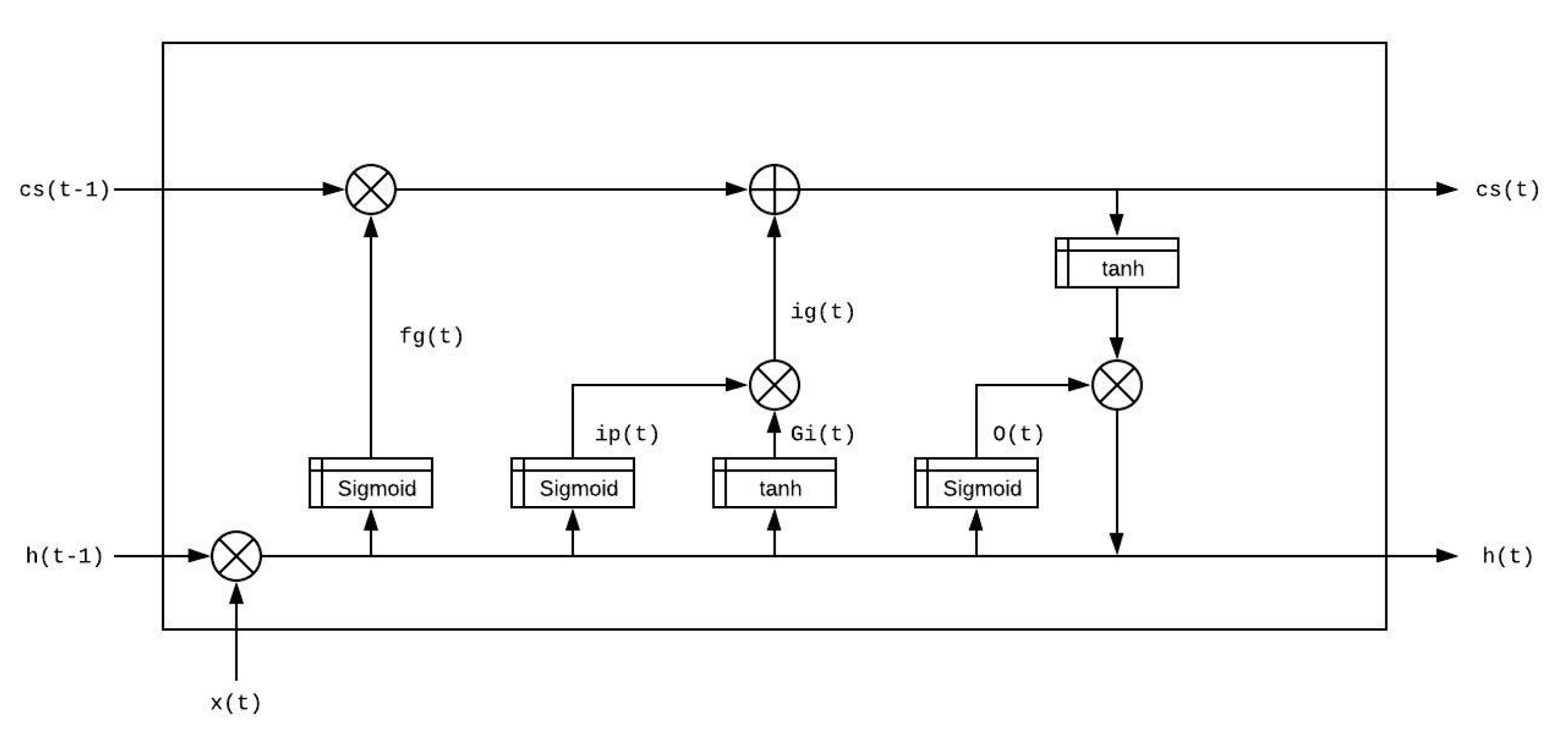
All RNNs are in the form of a chain of repeating modules of neural networks. In standard RNNs, this repeating module has a basic structure, such as a single tanh layer. However, LSTMs have a chain-like structure (called a carousel) with different repeating modules of the RNN. In the LSTM model, the repeating module has three different types of gates, namely, the forget gate, fg(t), the input gate, ip(t) × Gi(t), and the output gate, O(t), as shown in Figure 1.

3.2.2. Operation of LSTM

The first step in the LSTM model is to determine which piece of information to discard from the cell state (CS), considering the current input vector, x(t), and the previous short-term state vector, h(t − 1). The first step is accomplished using a sigmoid layer, which is called the “forget gate layer”. If the output of the sigmoid as an active function is 0, all previous CS (t − 1) values approaching 0 do not affect future results. However, if the output of the sigmoid as an active function is 1, the previous CS (t − 1) value is completely remembered in order to affect the next step for CS (t) and is given by the following equation [11,13,47,48]:

$$\mathrm{fg}\left(\mathrm{t}\right)=\mathsf{\sigma }·\left({\mathrm{w}}_{\mathrm{fg}}^{\mathrm{x}}·{\mathrm{x}}_{\mathrm{t}}+{\mathrm{w}}_{\mathrm{fg}}^{\mathrm{h}}·{\mathrm{h}}_{\mathrm{t}-1}+{\mathrm{b}}_{\mathrm{f}}\right),$$

(3)

In (3), ${\mathrm{w}}_{\mathrm{fg}}^{\mathrm{x}}$ and ${\mathrm{w}}_{\mathrm{fg}}^{\mathrm{h}}$ are the weighting vectors for the forget layer that are connected to the input vector denoted as x(t) and the previous short-term state h(t − 1), respectively. In addition, ${\mathrm{b}}_{\mathrm{f}}$ is defined as the bias for the forget layers.

The next step determines the new information to be stored in the CS, which is classified into two subprocesses. First, a sigmoid layer called the input gate layer, ip(t), determines which values to update. Next, a tanh layer creates a vector of new candidate values, Gi(t), that could be added to the state. In the next step, we combine these two steps to update the state ig(t), as shown in (4) to (6) [11,13,47,48]:

$$\mathrm{ip}\left(\mathrm{t}\right)=\mathsf{\sigma }·\left({\mathrm{w}}_{\mathrm{ip}}^{\mathrm{x}}·{\mathrm{x}}_{\mathrm{t}}+{\mathrm{w}}_{\mathrm{hi}}^{\mathrm{h}}·{\mathrm{h}}_{\mathrm{t}-1}+{\mathrm{b}}_{\mathrm{i}}\right)$$

(4)

$$\mathrm{Gi}\left(\mathrm{t}\right)=\tan \mathrm{h}·\left({\mathrm{w}}_{\mathrm{Gi}}^{\mathrm{x}}·{\mathrm{x}}_{\mathrm{t}}+{\mathrm{w}}_{\mathrm{Gi}}^{\mathrm{h}}·{\mathrm{h}}_{\mathrm{t}-1}+{\mathrm{b}}_{\mathrm{Gi}}\right)$$

(5)

$$\mathrm{ig}\left(\mathrm{t}\right)=\mathrm{ip}\left(\mathrm{t}\right)\otimes \mathrm{Gi}\left(\mathrm{t}\right)$$

(6)

where ${\mathrm{w}}_{\mathrm{ip}}^{\mathrm{x}}$ and ${\mathrm{w}}_{\mathrm{hi}}^{\mathrm{h}}$ are represented as weighting vectors for the input gate layer that are connected to the input vector denoted as x(t) and the previous short-term state h(t−1), respectively. The terms $b_i$ and $b_{Gi}$ are defined as the bias for the input gate layer.

The final decision step for the optimal CS (t) is based on the previous two steps, which can be readily obtained as follows [11,13,47,48]:

$$\mathrm{CS}\left(\mathrm{t}\right)=\mathrm{fg}\left(\mathrm{t}\right)\otimes \mathrm{CS}(\mathrm{t}-1)+\mathrm{ig}\left(\mathrm{t}\right)\otimes \mathrm{Gi}\left(\mathrm{t}\right).$$

(7)

First, the sigmoid function σ is determined by whether a CS outputs 0 or 1 for the neuron, denoted as O(t) [11,13,47,48]:

$$\mathrm{O}\left(\mathrm{t}\right)=\mathsf{\sigma }·\left({\mathrm{w}}_{\mathrm{O}}^{\mathrm{x}}·{\mathrm{x}}_{\mathrm{t}}+{\mathrm{w}}_{\mathrm{O}}^{\mathrm{h}}·{\mathrm{h}}_{\mathrm{t}-1}+{\mathrm{b}}_{\mathrm{O}}\right)$$

(8)

where ${\mathrm{w}}_{\mathrm{O}}^{\mathrm{x}}$ and ${\mathrm{w}}_{\mathrm{O}}^{\mathrm{h}}$ can be expressed as weighting vectors for the output gate that are connected to the input vector denoted as x(t) and the previous short-term state h(t − 1), respectively. In addition, b_o is defined as the bias for the output gate layer. Then, we apply the tanh function, which assigns weights to the values that are passed through, determining the level of importance, ranging from −1 to 1 of the CSs, and multiplying it by the output of the sigmoid gate denoted as h(t) [11,13,47,48]:

$$\mathrm{h}\left(\mathrm{t}\right)=\mathrm{O}\left(\mathrm{t}\right)\otimes \tan \mathrm{h}\left(\mathrm{CS}\right(\mathrm{t}\left)\right)$$

(9)

4. Proposed SolPV_ELA

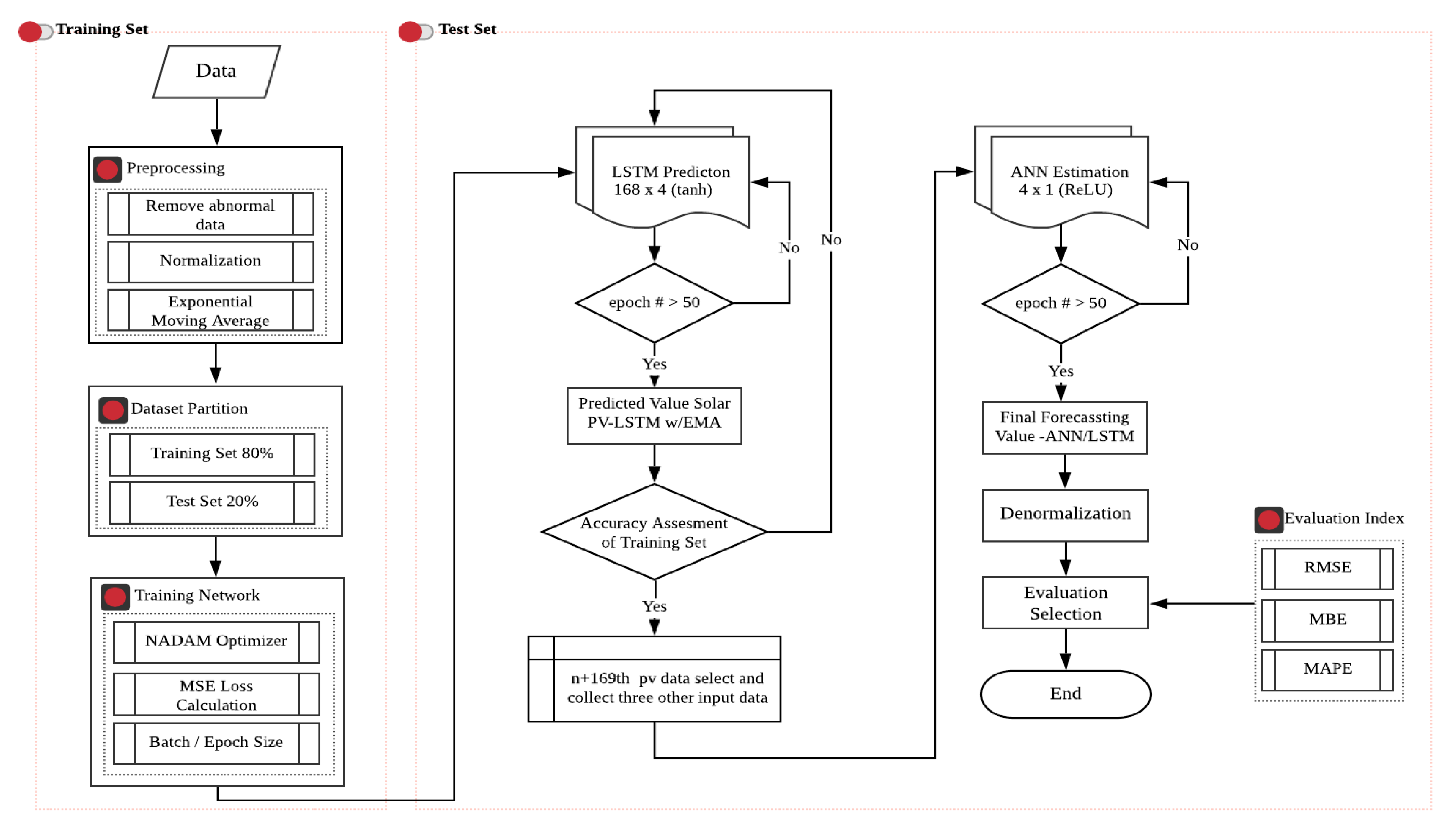
The proposed model (SolPV_ELA) consists of two stages, including a powerful two-stage neural network model for short-term forecasting of PV output power. The first stage uses the LSTM model to predict the target of the SPVG using the previous one week of data concerning the EMA. The second model uses the ANN model for accuracy estimation to obtain precise results using the previous data obtained from the LSTM model and three other types of input data at the target time. Through this approach, the first model (LSTM) is expected to have a value according to the previous trend, and the second model (ANN) obtains a value closer to the actual value by reflecting the input data at the desired time, as described in Figure 2.

4.1. Data Processing (Training and Testing Procedures)

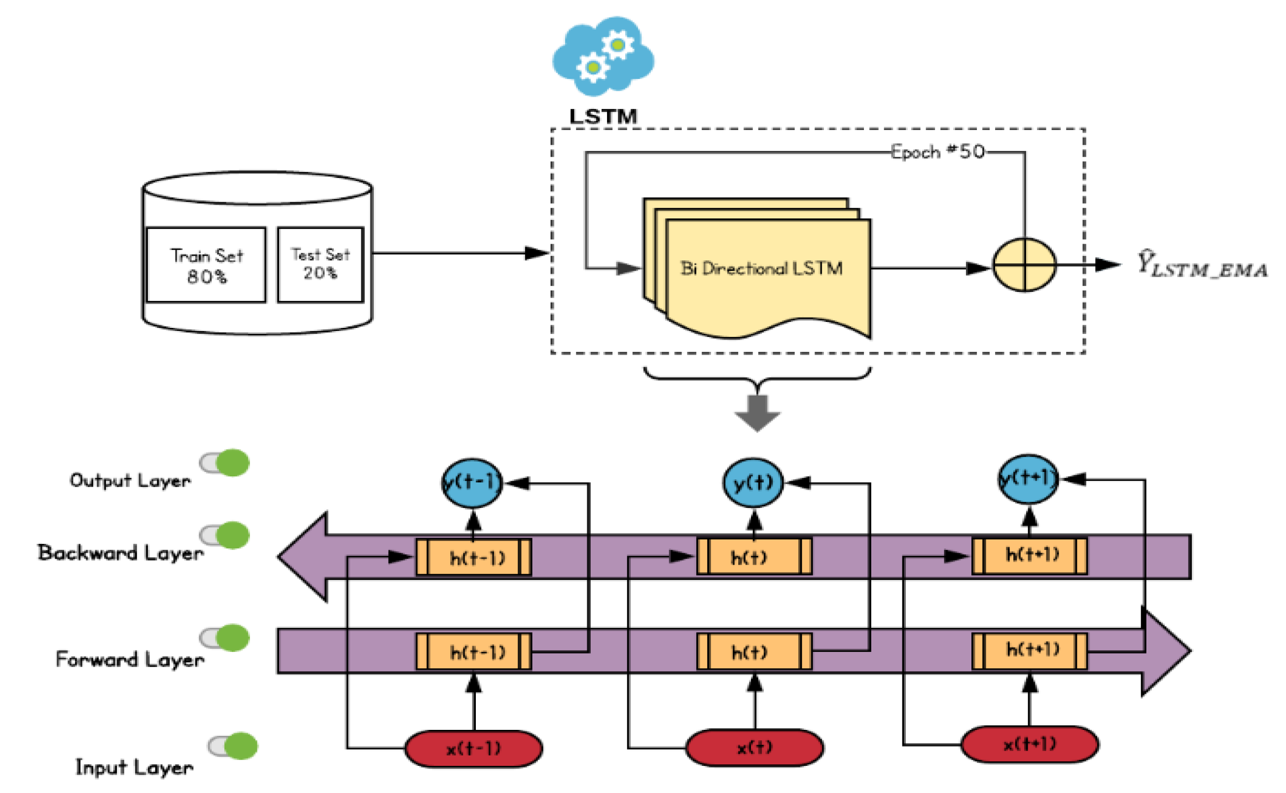
To forecast the output of one hour of solar PV recorded at a sampling interval of 1 h, the input data used a sequence of data consisting of four inputs of 168 h. In addition, 32,040 pieces of input data were generated using the given 32,208 data points, and each data point had the form of a 168 × 4 matrix. The dataset was divided into two subsets: 80% (25,632) as a training set, which is the subset for training the proposed model, and a 20% testing set, which is the subset for testing the proposed model from the trained data (6408), as shown in Figure 3.

4.2. LSTM Deep Learning Algorithm of the SolPV_ELA

As discussed in Chapter 2, the LSTM architecture effectively “extends” the memory of the RNN. The basic idea of a unidirectional LSTM model only preserves the past information because the inputs only originated from the previous sequence. However, the bidirectional LSTM (BD-LSTM) runs each training sequence forward and backward to separate two recurrent nets, both of which are connected to the same output layer, as presented in Figure 4. In other words, BD-LSTM does not require any prior knowledge or predesign due to the information being kept in both directions [49]. In this study, BD-LSTM was used to improve the accuracy of the prediction output by removing sequence classification problems [49]. The shape of the input data and output data was (168, 4) and (1, 1), respectively, and 64 nodes were arranged in each layer. Tanh was used for the activation function of the LSTM model, which is also known as the transfer function. This transfer function determines the output of the neural network, such as yes or no, which maps the resulting values between 0 and 1 or −1 and 1, as derived from the following equation:

$$Tanh\left(t\right)=\frac{2}{1+e^{-2t}}-1$$

(10)

4.3. ANN Estimation with Target Selection

We executed the learning rates for the training epoch at 50 in terms of the mean squared error (MSE), evaluating the training set using the optimizer function NADAM, which updates the weight parameters to minimize the loss function. To achieve high accuracy for the training set, the validation was set at 20% to check for the overfitting and underfitting of the training data.

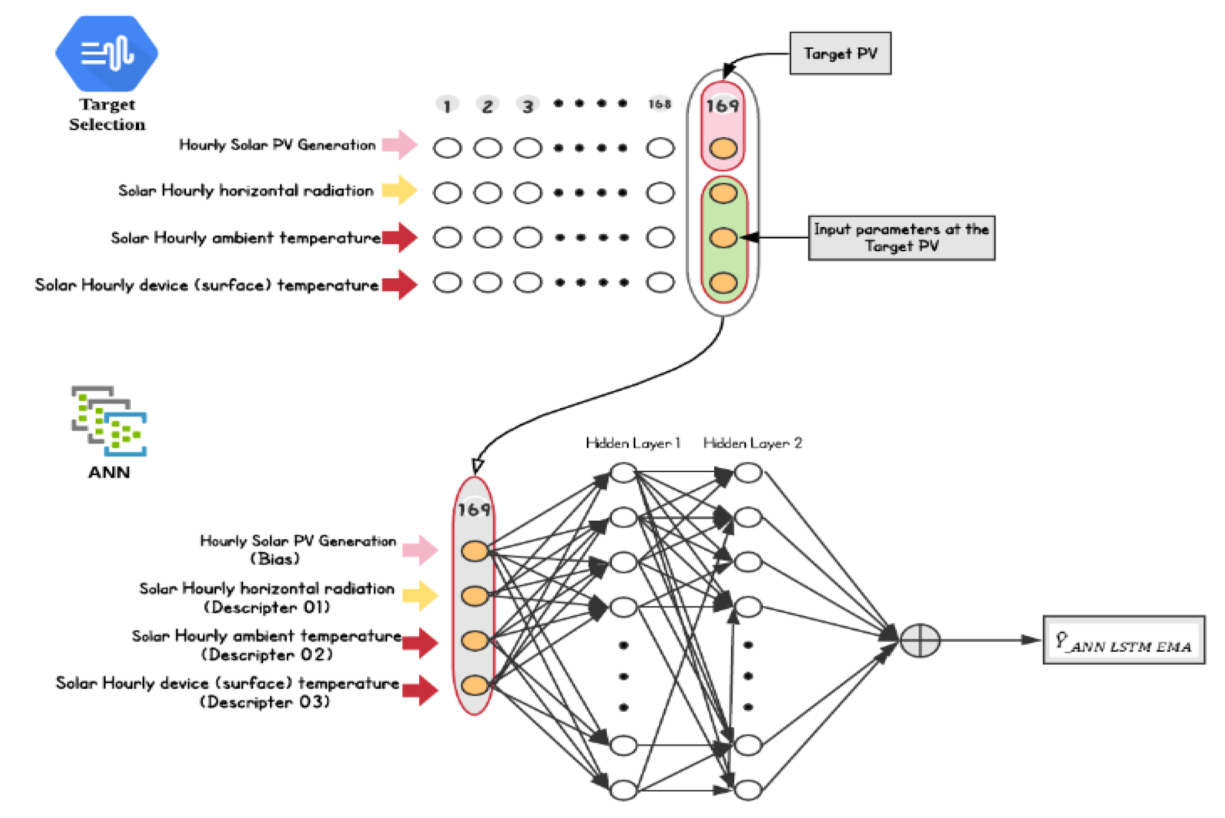
The trained data from the BD-LSTM prediction model might be able to reduce the MSE, which indicates that it could make a difference between the real and prediction values. However, problems still exist when environmental changes cannot be reflected at that time, which is due to unexpected trends such as a sudden weather change. To solve this issue, this study aimed to estimate the solar PV value of the predicted data from the BD-LSTM model to improve the accuracy by combining solar radiation and two temperature readings for the target time. The input and output layers of the ANN model are (4, 1) and (1, 1), respectively, as illustrated in Figure 5. Sixty-four nodes were placed in each layer, except for the output layer. The activation function of the node used the rectified linear unit that computes the function f(x) = max (0, x), which approaches zero as x < 0. In other words, the activation function is simply the thresholder at zero. Like the BD-LSTM model, the ANN model was trained for the first time when 50 training samples were collected using the loss function of the MSE and NADAM as the optimization function, with a 20% validation setting.

5. Case Study and Discussion

5.1. Data Description

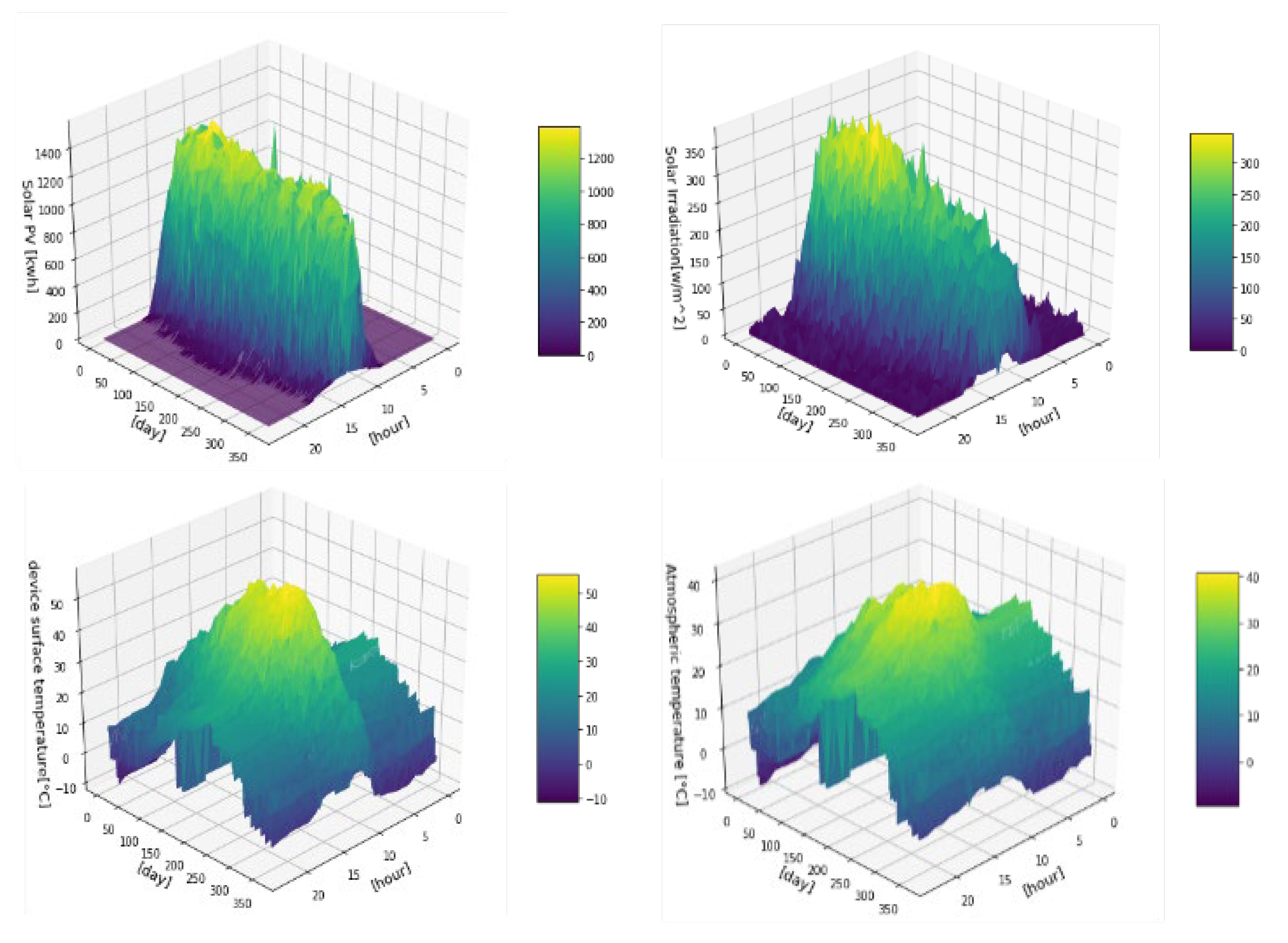
The testing data were acquired from a 1490 kWh (rated capacity) PV system that starts generating (usually between 6:00 and 19:00) when the sun rises in Yeonseong-gun, Gyeonggi-do, South Korea. The historical data were downloaded from the Korea Open Data Portal and then used as the input data from January 2015 to October 2018. To reduce the average prediction error, we excluded abnormal data and filled in missing data due to PV system failure and data loss. The original data consisted of four different parameters: SPVG (kWh), solar PV irradiation (W/m²), device surface temperature (°C; temperature range on the surface of the solar cell), and ambient temperature (°C; ambient temperature). In addition, the number of data points was 1342 (32,208 h), which was divided into training and testing datasets. Figure 6 depicts the SPVG (kWh), with the range of the highest density when the solar PV irradiation (W/m²) peaks (usually between 12:00 and 14:00). Furthermore, the device surface temperature (°C) has similar growth patterns in relation to the atmospheric temperature (°C). At peak times, the device surface temperature is 10 to 20 °C higher than the atmospheric temperature, with a similar seasonal pattern.

5.2. Performance Metrics in Terms of the Evaluation Index

Several evaluation indices are applied for the accuracy of SPVG. In this work, we measured the accuracy of the difference between the measured value and the predicted output using metrics such as the root mean squared error (RMSE in %), mean absolute percentage error (MAPE in %), and Pearson’s correlation coefficient (${\mathrm{R}}^2$).

The RMSE is the most common metric used to measure the accuracy of SPVG for continuous variables and can be defined as follows:

$$\mathrm{RMSE}=\sqrt{\frac{1}{\mathrm{N}}·{\displaystyle {\sum }_{\mathrm{i}=1}^{\mathrm{N}}}{({\mathrm{P}}_{\mathrm{i}}-\widehat{{\mathrm{P}}_{\mathrm{i}}})}^2}*100(\%)$$

(11)

${\mathrm{where}\mathrm{P}}_{\mathrm{i}}$ is the actual value, $\widehat{{\mathrm{P}}_{\mathrm{i}}}$ is the forecast value, and N represents the size of the test dataset for the i-th day in the test dataset.

The MAPE is also known as the mean absolute percentage deviation [26]. This index calculates the average error ratio in terms of a measure of prediction accuracy using the following formula:

$$\mathrm{M}\mathrm{A}\mathrm{P}\mathrm{E}= \frac{1}{\mathrm{N}} · {\displaystyle \sum }_{\mathrm{i}=1}^{\mathrm{N}}\left|\frac{{\mathrm{P}}_{\mathrm{i}}-\widehat{{\mathrm{P}}_{\mathrm{i}}}}{{\mathrm{P}}_{\mathrm{i}}}\right|$$

(12)

Pearson’s correlation coefficient (${\mathrm{R}}^2$) is the test statistic that measures the statistical relationship or association between two continuous variables [28]. If ${\mathrm{x}}_1,{\mathrm{x}}_2,\dots ,{\mathrm{x}}_n$ are the numbers of one set and ${\mathrm{y}}_1,{\mathrm{y}}_2,\dots ,{\mathrm{y}}_n$ are the numbers of another set, the coefficient of correlation between the two sets is as follows [50,51]:

$${\mathrm{R}}^2=\frac{{{\displaystyle \sum }}_1^{\mathrm{n}}{\mathrm{x}}_{\mathrm{i}}·{\mathrm{y}}_{\mathrm{i}}}{\sqrt{{{\displaystyle \sum }}_1^{\mathrm{n}}{\mathrm{x}}_{\mathrm{j}}^2}·\sqrt{{{\displaystyle \sum }}_1^{\mathrm{n}}{\mathrm{y}}_{\mathrm{j}}^2}}$$

(13)

This quantity must lie between −1 and 1. The Pearson correlation coefficient is calculated to measure the correlation between solar PV and three different input data for training. It identifies the most relevant parameters affecting the solar PV output power, as presented in Figure 7. Three input data were calculated: solar irradiation (0.92), device surface temperature (0.62), and ambient temperature (0.34), as depicted in Figure 7. All cases indicate a positive correlation, which has a positive effect on SPVG, and solar irradiation has the highest correlation compared to the other two cases. The device surface and ambient temperatures have a similar pattern distribution, whereas the device surface temperature is 0.28 better than the ambient temperature.

5.3. Performance Analysis

For a target hour, the SolPV_ELA (ELA) was verified by comparing it using different approaches: LSTM, CNN, and LSTM with an EMA (EL). We computed the performance indices, RMSE, MAE, and ${\mathrm{R}}^2$, to compare the performance of our proposed algorithm with that of the other models and present the results in

Table 2. Comparison of one-hour forecasting performance indices.

Type	R2	RMSE	MAE
ELA	0.96	83.26	45.24
EL	0.80	176.43	110.04
LSTM	0.87	142.41	85.04
CNN	0.80	185.07	105.97

.

Table 2 demonstrates that the proposed ELA model achieved much better performance. It had the highest correlation (0.96) compared to the other three options in terms of ${\mathrm{R}}^2.$ Furthermore, the approach ranking for RMSE was ELA (83.26), EL (176.43), LSTM (142.41), and CNN (185.07), whereas the approach ranking for MAE was ELA (45.24), LSTM (85.04), EL (110.04), and CNN (105.97). According to these results, the forecasting results of the ELA are almost twice as accurate as the other methods. In addition, the ELA performance differs from the worst case (CNN) by 102 for RMSE and 60 for MAE. Table 2 indicates that the EMA did not reduce the error rate for one-hour-ahead PV forecasting, as revealed by the comparative performances of EL and LSTM.

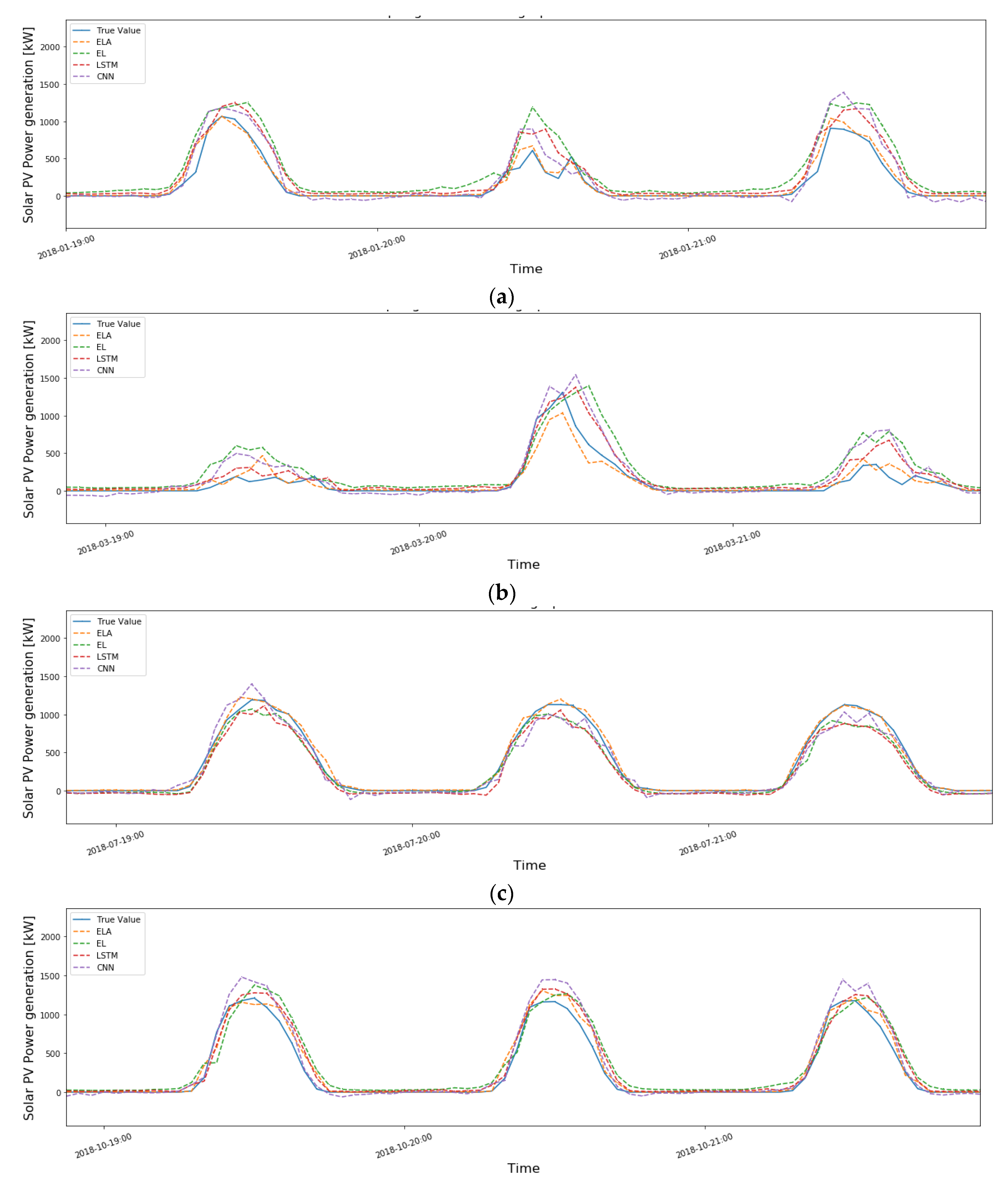
Figure 8 illustrates that the ELA model has high accuracy and high stability under different weather conditions in all four seasons. In Case I, winter, the mid-day shape was broken by a passing cloud. The ELA model still improves the predicted output better than the other options. Cases III and IV have normal condition patterns, while two days in Case II, winter, have a lower PV, and the shape was distorted by the rainy season. However, the ELA model can still track real data under bad weather conditions.

6. Conclusions

This paper proposed a new approach (ELA) to improve the accuracy of a two-step model by estimating the ANN of four types of input data at the designated time based on LSTM prediction modeling with EMA smoothing preprocessing. The ELA model was validated using real input data that originated from the Korea Open Data Portal for January 2015 to October 2018. These input data were used to forecast the output of one-hour solar PV power recorded at a sampling interval of 1 h.

The numerical results indicated that the ELA model outperforms (R² = 0.16, RMSE = 102, MAE = 60) the worst case of the CNN model. The other neural-network-based solutions (CNN, LSTM, and EL) could not perform better than our proposed theory-based method (i.e., the ELA model) due to insufficient data and no capability to leverage the priori knowledge. Furthermore, the performance of the ELA model was visualized to better predict the performance in different cases for four seasons, which provides reliable PV power forecasting for an actual power plant. In future studies, we plan to consider how to combine our method with neural-network-based methods so that a data-driven gain can enhance the theoretical advantage.

References

- IEA. Renewables 2018: Analysis and Forecasts to 2023. October 2018. Available online: https://www.iea.org/reports/renewables-2018 (accessed on 2 December 2019).
- Mordor Intelligence, South Korea Solar Photovoltaic (PV) Market Outlook to 2022. 2019. Available online: https://www.mordorintelligence.com/industry-reports/south-korea-solar-power-market-industry (accessed on 8 January 2020).
- South Korean Ministry of Trade, Industry, and Energy, Press Releases, Ministry Announces 7th Basic Plan for Electricity Supply and Demand, 14 December 2017. Available online: https://www.kpx.or.kr/eng/selectBbsNttView.do?key=328&bbsNo=199&nttNo=14547& (accessed on 8 January 2020).
- Da Silva, A.P.C.; Renga, D.; Meo, M.; Marsan, M.A. The impact of quantization on the design of solar power systems for cellular base stations. IEEE Trans. Green Commun. Netw. 2017, 2, 260–274. [Google Scholar] [CrossRef]
- IRENA. Future of Solar Photovoltaic: Deployment, Investment, Technology, Grid Integration and Socio-Economic Aspects (A Global Energy Transformation: Paper); International Renewable Energy Agency: Abu Dhabi, UAE, 2019; Available online: https://www.irena.org/-/media/Files/IRENA/Agency/Publication/2019/Nov/IRENA_Future_of_Solar_PV_2019.pdf (accessed on 8 January 2020).
- Zhou, H.; Zhang, Y.; Yang, L.; Liu, Q.; Yan, K.; Du, Y. Short-term photovoltaic power forecasting based on long short-term memory neural network and attention mechanism. IEEE Access 2019, 7, 78063–78074. [Google Scholar] [CrossRef]
- Das, U.K.; Tey, K.S.; Seyedmahmoudian, M.; Mekhilef, S.; Idris, M.Y.I.; van Deventer, W.; Horan, B.; Stojcevski, A. Forecasting of photovoltaic power generation and model optimization: A review. Renew. Sustain. Energy Rev. 2018, 81, 912–928. [Google Scholar] [CrossRef]
- Wan, C.; Zhao, J.; Song, Y.; Xu, Z.; Lin, J.; Hu, Z. Photovoltaic and solar power forecasting for smart grid energy management. CSEE J. Power Energy Syst. 2015, 1, 38–46. [Google Scholar] [CrossRef]
- Chai, M.; Xia, F.; Hao, S.; Peng, D.; Cui, C.; Liu, W. PV power prediction based on LSTM with adaptive hyperparameter adjustment. IEEE Access 2019, 7, 115473–115486. [Google Scholar] [CrossRef]
- Liu, J.; Fang, W.; Zhang, X.; Yang, C. An improved photovoltaic power forecasting model with the assistance of aerosol index data. IEEE Trans. Sustain. Energy 2015, 6, 434–442. [Google Scholar] [CrossRef]
- Gao, M.; Li, J.; Hong, F.; Long, D. Day-ahead power forecasting in a large-scale photovoltaic plant based on weather classification using LSTM. Energy 2019, 187, 115838. [Google Scholar] [CrossRef]
- Huang, C.; Kuo, P. Multiple-input deep convolutional neural network model for short-term photovoltaic power forecasting. IEEE Access 2019, 7, 74822–74834. [Google Scholar] [CrossRef]
- Wang, K.; Qi, X.; Liu, H. Photovoltaic power forecasting based LSTM convolutional network. Energy 2019, 189, 116225. [Google Scholar] [CrossRef]
- Lopes, F.; Silva, H.; Salgado, R.; Cavaco, A.; Canhoto, P.; Collares-Pereira, M. Short-term forecasts of GHI and DNI for solar energy systems operation: Assessment of the ECMWF integrated forecasting system in southern Portugal. Sol. Energy 2018, 170, 14–30. [Google Scholar] [CrossRef]
- Miller, S.D.; Rogers, M.A.; Haynes, J.M. Short-term solar irradiance forecasting via satellite/model coupling. Sol. Energy 2017, 168, 102–117. [Google Scholar] [CrossRef]
- Li, G.; Wang, H.; Zhang, S.; Xin, J.; Liu, H. Recurrent neural networks based photovoltaic power forecasting approach. Energies 2019, 12, 2538. [Google Scholar] [CrossRef]
- Inman, R.H.; Pedro, H.T.; Coimbra, C.F. Solar forecasting methods for renewable energy integration. Prog. Energy Combust. Sci. 2013, 39, 535–576. [Google Scholar] [CrossRef]
- Li, Y.; Niu, J. Forecast of power generation for grid-connected photovoltaic system based on Markov chain. In Proceedings of the 2009 Asia-Pacific Power and Energy Engineering Conference (APPEEC’09), Wuhan, China, 27–31 March 2009; pp. 1–4. [Google Scholar]
- Jang, H.S.; Bae, K.Y.; Park, H.; Sung, D.K. Solar power prediction based on satellite images and support vector machine. IEEE Trans. Sustain. Energy 2016, 7, 1255–1263. [Google Scholar] [CrossRef]
- Song, J.; Krishnamurthy, V.; Kwasinski, A.; Sharma, R. Development of a Markov-chain-based energy storage model for power supply availability assessment of photovoltaic generation plants. IEEE Trans. Sustain. Energy 2013, 4, 491–500. [Google Scholar]
- Miao, S.; Ning, G.; Gu, Y.; Yan, J.; Ma, B. Markov chain model for solar farm generation and its application to generation performance evaluation. J. Clean. Prod. 2018, 186, 905–917. [Google Scholar] [CrossRef]
- Elminir, H.K.; Azzam, Y.A.; Younes, F.I. Prediction of hourly and daily diffuse fraction using neural network, as compared to linear regression models. Energy 2017, 32, 1513–1523. [Google Scholar] [CrossRef]
- Sulaiman, S.I.; Rahman, T.K.A.; Musirin, I.; Shaari, S. Artificial neural network versus linear regression for predicting grid-connected photovoltaic system output. In Proceedings of the 2012 IEEE International Conference on Cyber Technology in Automation, Control, and Intelligent Systems (CYBER), Bangkok, Thailand, 27–31 May 2012; pp. 170–174. [Google Scholar]
- Poolla, C.; Ishihara, A.K. Localized solar power prediction based on weather data from local history and global forecasts. In Proceedings of the 2018 IEEE 7th World Conference Photovoltaic Energy Conversion (WCPEC) (Joint Conference 45th IEEE PVSC, 28th PVSEC & 34th EU PVSEC), Waikoloa Village, HI, USA, 10–15 June 2018; pp. 2341–2345. [Google Scholar]
- Saghafian, B.; Anvari, S.; Morid, S. Effect of southern oscillation index and spatially distributed climate data on improving the accuracy of artificial neural network, adaptive neuro–fuzzy inference system and K-nearest neighbor streamflow forecasting models. Expert Syst. 2013, 30, 367–380. [Google Scholar] [CrossRef]
- Lee, W.; Kim, K.; Park, J.; Kim, J.; Kim, Y. Forecasting solar power using long-short term memory and convolutional neural networks. IEEE Access 2018, 6, 73068–73080. [Google Scholar] [CrossRef]
- Wang, Y.; Liao, W.; Chang, Y. Gated recurrent unit network-based short-term photovoltaic forecasting. Energies 2018, 11, 2163. [Google Scholar] [CrossRef]
- Sheng, H.; Xiao, J.; Cheng, Y.; Ni, Q.; Wang, S. Short-term solar power forecasting based on weighted Gaussian process regression. IEEE Trans. Ind. Electron. 2018, 65, 300–308. [Google Scholar] [CrossRef]
- Du, P. Ensemble machine learning-based wind forecasting to combine NWP output with data from weather Station. IEEE Trans. Sustain. Energy 2019, 10, 2133–2141. [Google Scholar] [CrossRef]
- Liu, Z.; Zhang, Z. Solar forecasting by K-nearest neighbors method with weather classification and physical model. In Proceedings of the 2016 North American Power Symposium (NAPS), Denver, CO, USA, 18–20 September 2016; pp. 1–6. [Google Scholar]
- Abuella, M.; Chowdhury, B. Solar power probabilistic forecasting by using multiple linear regression analysis. In Proceedings of the SoutheastCon 2015, Fort Lauderdale, FL, USA, 9–12 April 2015; pp. 1–5. [Google Scholar]
- Gensler, A.; Henze, J.; Sick, B.; Raabe, N. Deep learning for solar power forecasting—An approach using AutoEncoder and LSTM neural networks. In Proceedings of the 2016 IEEE International Conference on Systems, Man, and Cybernetics (SMC), Budapest, Hungary, 9–12 October 2016; pp. 002858–002865. [Google Scholar]
- Zeng, J.; Qiao, W. Short-term solar power prediction using a support vector machine. Renew. Energy 2013, 52, 118–127. [Google Scholar] [CrossRef]
- Li, R.; Wang, H.N.; He, H.; Cui, Y.M.; Du, Z.L. Support vector machine combined with k-nearest neighbors for solar flare forecasting. Chin. J. Astron. Astrophys. 2007, 7, 441. [Google Scholar] [CrossRef]
- Qiu, X.; Zhang, L.; Ren, Y.; Suganthan, P.N.; Amaratunga, G. Ensemble deep learning for regression and time series forecasting. In Proceedings of the 2014 IEEE Symposium on Computational Intelligence in Ensemble Learning (CIEL), Orlando, FL, USA, 9–12 December 2014; pp. 1–6. [Google Scholar]
- Muzumdar, A.; Modi, C.N.; Madhu, G.M.; Vyjayanthi, C. Analyzing the feasibility of different machine learning techniques for energy imbalance classification in smart grid. In Proceedings of the2019 10th International Conference on Computing, Communication and Networking Technologies (ICCCNT), Kanpur, India, 6–8 July 2019; pp. 1–6. [Google Scholar]
- Wang, J.; Li, P.; Ran, R.; Che, Y.; Zhou, Y. A short-term photovoltaic power prediction model based on the gradient boost decision tree. Appl. Sci. 2018, 8, 689. [Google Scholar] [CrossRef]
- Chaturvedi, D.K.; Isha, I. Solar power forecasting: A review. Int. J. Comput. Appl. 2016, 145, 28–50. [Google Scholar]
- Zhu, H.; Li, X.; Sun, Q.; Nie, L.; Yao, J.; Zhao, G. A power prediction method for photovoltaic power plant based on wavelet decomposition and artificial neural networks. Energies 2015, 9, 11. [Google Scholar] [CrossRef]
- Al-Dahidi, S.; Ayadi, O.; Alrbai, M.; Adeeb, J. Ensemble approach of optimized artificial neural networks for solar photovoltaic power prediction. IEEE Access 2019, 7, 81741–81758. [Google Scholar] [CrossRef]
- Sun, Y.; Venugopal, V.; Brandt, A.R. Convolutional Neural Network for Short-term Solar Panel Output Prediction. In Proceedings of the 2018 IEEE 7th World Conference on Photovoltaic Energy Conversion (WCPEC) (A Joint Conference of 45th IEEE PVSC, 28th PVSEC & 34th EU PVSEC), Waikoloa Village, HI, USA, 10–15 June 2018; pp. 2357–2361. [Google Scholar]
- Kim, D.; Hwang, S.; Kim, J. Very Short-Term Photovoltaic Power Generation Forecasting with Convolutional Neural Networks. In Proceedings of the 2018 International Conference on Information and Communication Technology Convergence (ICTC), Jeju, Korea, 19 November 2018; pp. 1310–1312. [Google Scholar]
- Sodsong, N.; Yu, K.M.; Ouyang, W. Short-Term Solar PV Forecasting Using Gated Recurrent Unit with a Cascade Model. In Proceedings of the 2019 International Conference on Artificial Intelligence in Information and Communication (ICAIIC), Okinawa, Japan, 11–13 February 2019; pp. 292–297. [Google Scholar]
- Neo, Y.Q.; Teo, T.T.; Woo, W.L.; Logenthiran, T.; Sharma, A. Forecasting of photovoltaic power using deep belief network. In Proceedings of the TENCON 2017—2017 IEEE Region 10 Conference, Penang, Malaysia, 5–8 November 2017; pp. 1189–1194. [Google Scholar]
- Brockwell, P.J.; Davis, R.A. Introduction to Time Series and Forecasting, 3rd ed.; Springer: Berlin, Germany, 2016. [Google Scholar]
- Hunter, J.S. The exponentially weighted moving average. Qual. Technol. 1986, 18, 203–207. [Google Scholar] [CrossRef]
- Zaouali, K.; Rekik, R.; Bouallegue, R. Deep Learning Forecasting Based on Auto-LSTM Model for Home Solar Power Systems. In Proceedings of the 2018 IEEE 20th International Conference on High Performance Computing and Communications, Exeter, UK, 28–30 June 2018. [Google Scholar]
- Lai, G.; Chang, W.C.; Yang, Y.; Liu, H. Modeling long- and short-term temporal patterns with deep neural networks. In Proceedings of the 41st International ACM SIGIR Conference on Research & Development in Information Retrieval, Ann Arbor, MI, USA, 8–12 June 2018; pp. 95–104. [Google Scholar]
- Cui, Z.; Ke, R.; Wang, Y. Deep Stacked Bidirectional and Unidirectional LSTM Recurrent Neural Network for Network-wide Traffic Speed Prediction. In Proceedings of the 6th International Workshop on Urban Computing (UrbComp 2017), Halifax, NS, Canada, 14 August 2017. [Google Scholar]
- Wiener, N. Extrapolation, Interpolation, and Smoothing of Stationary Time Series: With Engineering Applications; MIT Press: Cambridge, MA, USA, 1964; p. 163. [Google Scholar]
- Zhong, J.; Liu, L.; Sun, Q.; Wang, X. Prediction of photovoltaic power generation based on general regression and back propagation neural network. Energy Procedia 2018, 152, 1224–1229. [Google Scholar]
Figure 1.
Structure of long short-term memory (LSTM) model: the repeating module has three different types of gates, namely, the forget gate, fg(t); the input gate, ig(t) (=ip(t) × Gi(t)); the output gate, O(t).
Figure 2.
Flow chart of the two-stage neural network model (SolPV_ELA) for short-term forecasting of photovoltaic (PV) output power.