Development of Attached Cavitation at Very Low Reynolds Numbers from Partial to Super-Cavitation
by
 , , , and
Florent Ravelet
* ,
,
Amélie Danlos
,
Farid Bakir
,
Kilian Croci
,
Sofiane Khelladi
 and
and
Christophe Sarraf
Arts et Metiers Institute of Technology, CNAM, LIFSE, HESAM University, 75013 Paris, France
*
Author to whom correspondence should be addressed.
Appl. Sci. 2020, 10(20), 7350; https://doi.org/10.3390/app10207350
Submission received: 1 October 2020
/
Revised: 13 October 2020
/
Accepted: 16 October 2020
/
Published: 20 October 2020
(This article belongs to the Special Issue New Advances of Cavitation Instabilities)
Abstract
:The present study focuses on the inception, the growth, and the potential unsteady dynamics of attached vapor cavities into laminar separation bubbles. A viscous silicon oil has been used in a Venturi geometry to explore the flow for Reynolds numbers ranging from to . Special care has been taken to extract the maximum amount of dissolved air. At the lowest Reynolds numbers the cavities are steady and grow regularly with decreasing ambient pressure. A transition takes place between and for which different dynamical regimes are identified: a steady regime for tiny cavities, a periodical regime of attached cavity shrinking characterized by a very small Strouhal number for cavities of intermediate sizes, the bursting of aperiodical cavitational vortices which further lower the pressure, and finally steady super-cavitating sheets observed at the lowest of pressures. The growth of the cavity with the decrease of the cavitation number also becomes steeper. This scenario is then well established and similar for Reynolds numbers between and .
1. Introduction
The presence of small separation bubbles close to the leading edge of a profile or to the summit of a wedge provides favorable conditions for the attachment of vaporous cavities when lowering the absolute pressure. The fundamentals of sheet cavitation inception can be found for instance in the classical books of C. E. Brennen [1] or J.-P. Franc [2]. The inception of such “sheet” cavitation has been for instance studied in Refs. [3,4,5,6,7] on smooth axi-symmetric bodies, on propellers blades or on foils. Moreover, a recent review of the different sheet cavitation inception mechanisms can be found in Ref. [8].
Once the inception of cavitation has occurred, for lower pressures the attached sheet cavities usually grow and become unstable, leading to periodical cloud shedding [9,10,11]. Partial and cloud cavitations are associated with a vapor region that extends over a part of the cavitating body [2]. At very low pressures, one can observe super-cavitation, consisting of a large and stable vapor cavity that extends beyond the body and closes in the liquid. In that case the pressure fluctuations are usually small [12,13]. For turbomachinery applications, the unsteady dynamics of attached sheets may be responsible for an increase of noise and vibrations and is of crucial importance for system instabilities [14,15]. The instabilities of attached sheet cavitation are attributed to two main phenomena: the formation of a re-entrant jet which is governed by inertia [16], and a bubbly shock propagation mechanism [17]. These two mechanisms have been recently subject to extensive studies, at least for very large Reynolds numbers, in water [18,19,20,21,22]. The cavitation in that case arises on a turbulent flow background.
The current studies that are conducted in the LIFSE (Laboratory of Fluid Engineering and Energetic Systems) deal with cavitating flows at very low Reynolds numbers, i.e., in laminar or transitional regimes. To the best of our knowledge, only very few studies have been carried out on hydrodynamic cavitation [23,24] or flow-induced degassing [25,26] in laminar flows. The main goal of the present study is to identify and compare potential unsteady regimes in viscosity-dominated cavitating flows to the aforementioned regimes observed in turbulent flows. In the present study, viscous silicone oil is used in a well-documented Venturi-type geometry [10]. In a first study conducted in our laboratory (Croci et al. (2018, 2019) [27,28]), the main features of the multiphase structures that arise have been observed from a qualitative point of view, using silicone oil. Silicone oil can dissolve much more air than water under the same thermodynamical conditions [29,30]. In the work of Croci et al. (2018, 2019) [27,28] the oil was saturated with air at atmospheric pressure. Single-phase numerical simulations have been performed additionally to illustrate the flow topology and to estimate the threshold for cavitation inception. As a result, different types of cavities are observed: tadpoles that attach on the lateral wall [27], sheets that attach on the Venturi slope and top-tadpoles that attach on the opposite side of the vein. The numerical simulations, pressure measurements and high-speed visualizations suggest to attribute the tadpoles to degassing, the main cavity sheet to cavitation, and the top-tadpoles to a secondary flow separation that captures air [28].
In the present article, experiments were performed with degassed silicone oil, to remove air bubbles and to get rid of degassing phenomena [25,26,31]. As a result, only central attached sheet cavities are present in the flow. Quantitative measurements based on high-speed visualizations are performed in order to characterize the evolution of the shapes, lengths and temporal features of the attached sheets with a decrease of the ambient pressure at constant Reynolds numbers , both in steady laminar flow (at ) and in transitional flows (up to ).
Section 2 is dedicated to the presentation of the experimental setup. The test-bench and the protocol are described in Section 2.1; the main parameters and the post-processing of the high-speed movies are discussed in Section 2.2; and a few numerical results giving insight into the single-phase flow topology and about its transition are recalled in Section 2.3.
The main results are presented in Section 3. The differences between experiments with air-saturated and degassed oil are illustrated in Section 3.1. The different regimes are presented in Section 3.2 and are quantitatively characterized in Section 3.3. Concluding remarks are then given in Section 4.
2. Experimental Study Overview
2.1. Experimental Test-Bench and Protocol
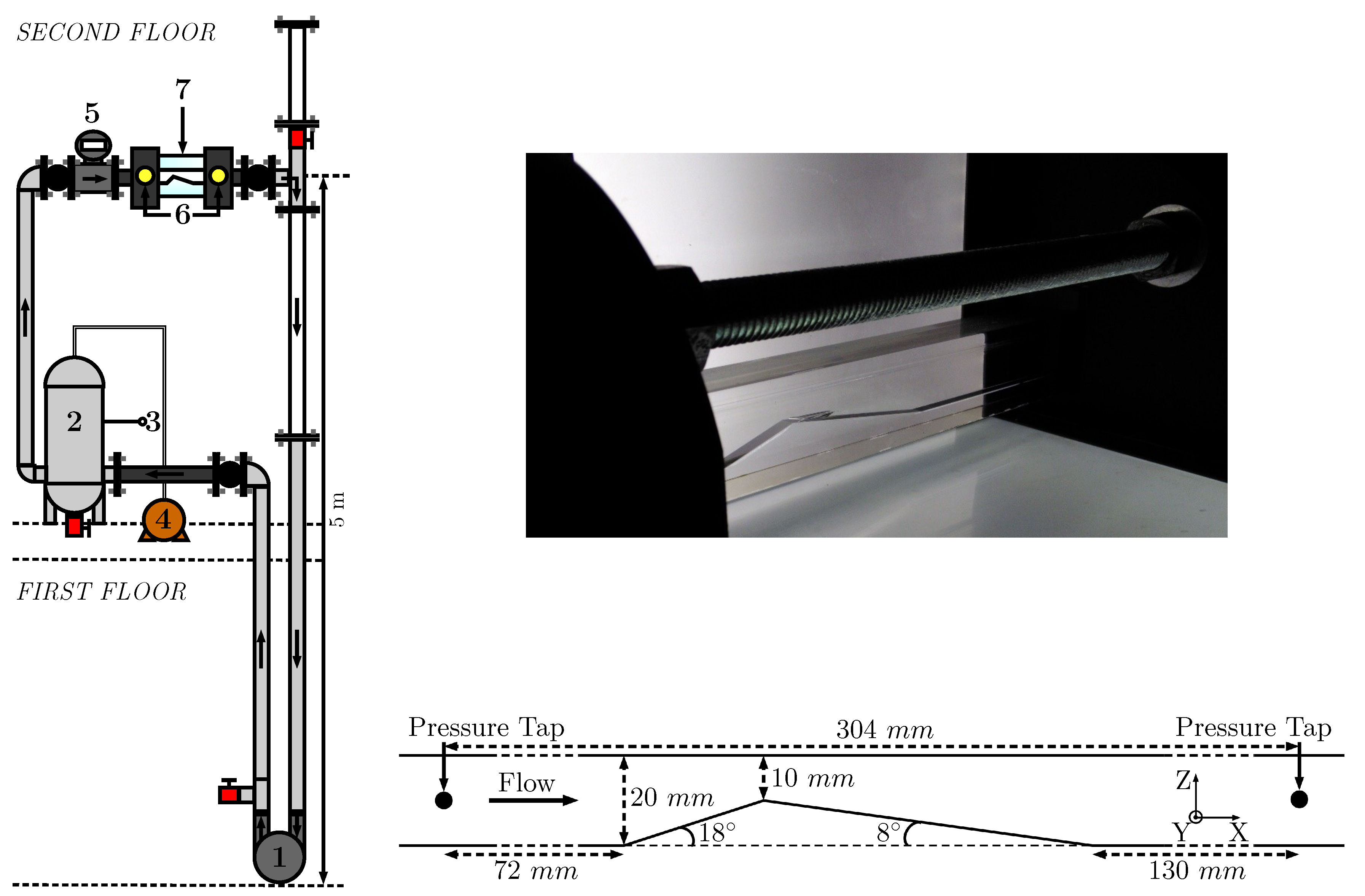
The experiments are conducted in a test-bench of the LIFSE facilities especially designed to study cavitation in silicone oils (see Figure 1). A Pollard MPLN 142 volumetric pump (1) impels the silicone oil in the loop. A tank of 100 liters (2) is equipped with a temperature sensor ThermoEst PT100 (3). The tank is connected to compressed air supply or to a vacuum pump (4). The oil then flows in a 40 mm inner diameter pipe and through an ultrasonic flowmeter KHRONE Optisonic 3400 (5) placed m upstream of the test section (7). The inlet and outlet pressures are monitored with two JUMO dTrans p30 pressure sensors (6).
The test section consists of a Venturi geometry with convergent/divergent angles of respectively and [10]. It presents an inlet section mm and a square section at the throat mm. Both side and top visualizations are possible. Two round-to-rectangle contraction nozzles with an area ratio of are placed on each sides of the test section to connect it to the pipe system.
All experiments are realized following a protocol to eliminate a maximum of dissolved air. The pressure in the setup is first decreased to an absolute pressure of ≃70 mbar, then the oil is kept circulating for this pressure at slow velocity during two hours, while removing periodically the air that accumulates in the vertical tube situated above the outlet of the test section and visible on the top part of the sketch on the left in Figure 1. The measurements are then operated at roughly constant Reynolds number, increasing progressively the pressure in the test-bench.
2.2. Control Parameters, Flow Visualization and Measured Quantities
The inlet and outlet test section absolute pressure, named and , are measured with two pressure transducers located respectively at 103 mm upstream and 201 mm downstream of the Venturi throat. The discharge throat velocity at is computed from flow rate measurements. The viscosity and density have been measured as a function of the temperature [32].
The following dimensionless numbers are defined based on these values: a Reynolds number , an inlet and an outlet cavitation numbers and and a capillary number . The definition of these parameters, together with the ranges that have been explored in the present article and the associated uncertainties, can be found in Table 1. Please note that the outlet cavitation number has not been considered in the previous study [28]. It is used in the present article as it seems to be more significant for analyzing the results. We also introduce a dimensionless pressure coefficient . Please note that is simply .
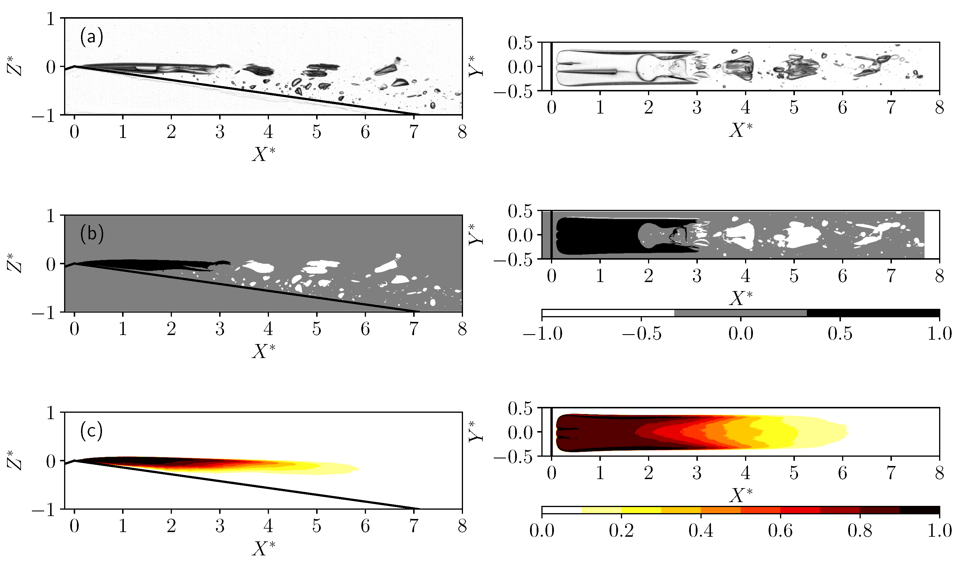
Two Optronis CR1000x3 high-speed cameras are used to visualize the cavities. The two cameras allow synchronized pictures from the top and from the side of the test section, with a field of view of pixels. Image sequences of 2 to 3 seconds are recorded at 1500 Hz or 1000 Hz. The flow is illuminated from the bottom and the backside with two continuous white LED plate from Phlox and consequently, the gaseous cavities appear as black features in the images. A typical result obtained at is displayed in Figure 2.
The height of the Venturi throat mm is chosen as the reference length scale for the dimensionless coordinates , and (see also the bottom right part in Figure 1 for the definition of the coordinate system). The origin of the positions is on top of the wedge, in the symmetry plane of the flow vein. The diverging part of the Venturi section thus extends from to ; the two side walls are at and the upper flat wall is at .
Time series of 3000 images are recorded for each experiment. A background reference image is also recorded with the same cameras setting, while the flow is at rest. The instantaneous images are then processed with Python, using the scipy.ndimage and scikit-image libraries [33] in the following way, based on Morphological Image Processing [34]:
- The images are converted to matrices of floats, the background is subtracted and the result is normalized by the background reference image, giving the ith normalized image of the time series (see Figure 2a). The gaseous features that are darker than the background have then gray-level values in the range .
- Image is then binarized with a threshold of : which gives the position of the interfaces between liquid and cavities with a dimensionless accuracy of (see Figure 3b for a gray-level profile on a normalized image).
- The holes that could remain inside the cavities are then filled with an algorithm based on invading the complementary of from the outer boundary of the image with binary dilations. Holes are not connected to the boundary and are therefore not invaded. The result is the complementary subset of the invaded region. A filled binary image is obtained.
- The features are then labeled, and their properties are measured with the scikit-image functions measure.label() and measure.regionprops(). A filter on the bounding box of the labeled regions is then used to keep the region that is the closest to the Venturi throat, resulting in a binary image containing a closed and filled representation of the cavity that is attached to the throat . This process is illustrated in Figure 2b where is displayed.
- The mean and standard deviation of the time series of the filtered images are then computed. The mean image for the series at , and is displayed in Figure 2c.
The length of the attached cavities is then measured on the mean images of the side view, using a threshold . This value corresponds to the region of space where the attached sheet is present on of the time series. For the case illustrated in Figure 2, it gives a length . Varying the threshold between and —see the colorbar in Figure 2c—leads to a variation of on the measure of which is a relative variation of .
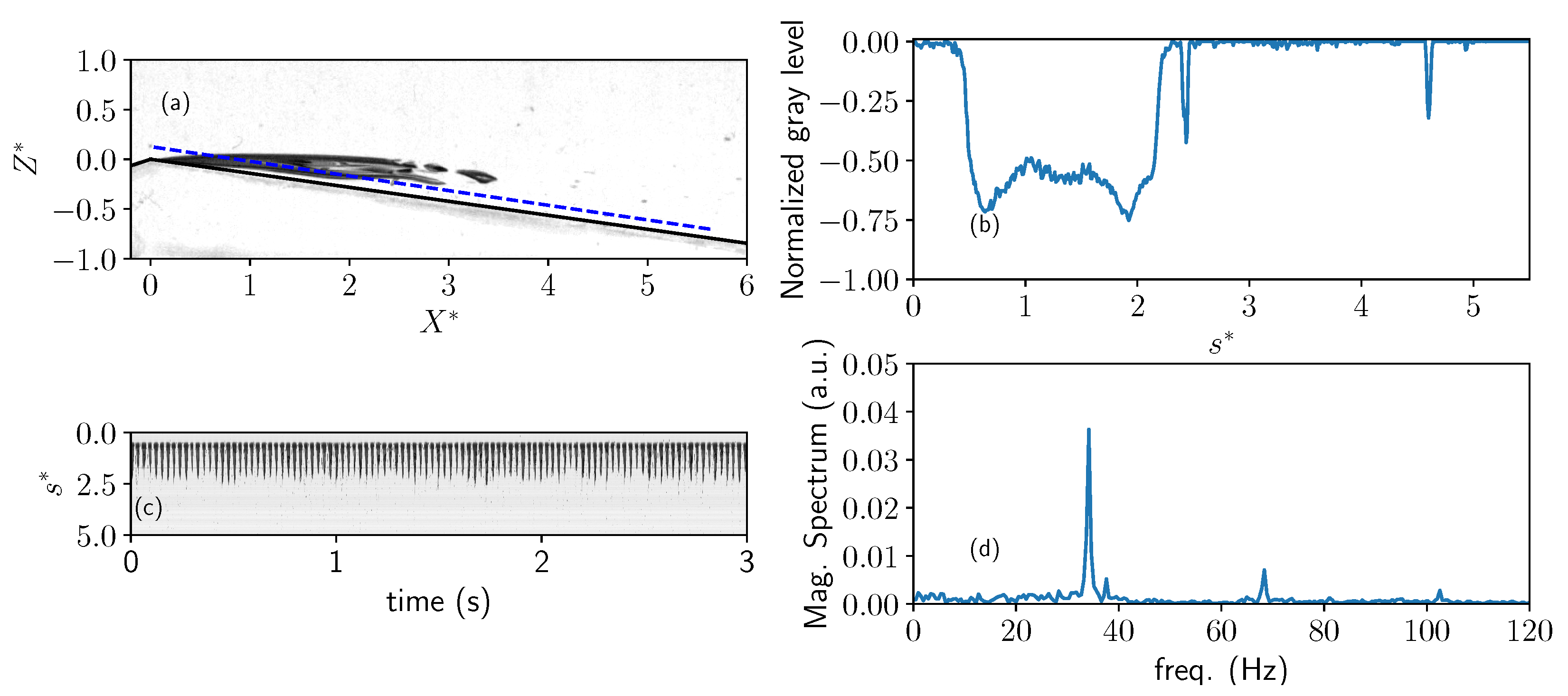
Spatio-temporal diagrams are also extracted along various lines in the normalized images in order to characterize the dynamics of the cavities and to measure the frequencies of periodical shrinking or shedding of the cavities. The post-processing is illustrated in Figure 3, where the spatio-temporal diagram is extracted along a line parallel to the Venturi diverging wall, about 1 mm above. The spatio-temporal matrix of gray levels is averaged along the spatial coordinate to give a time signal, from which the magnitude spectrum is computed. The main result which is the frequency of the main peak in the spectrum—if existing—is insensitive to the precise choice of the line: similar diagrams and the same frequency are obtained for horizontal or inclined lines at various heights, providing these lines cross the attached sheet. The best signal-to-noise ratio is obtained for the line displayed in Figure 3.
2.3. Numerical Highlights and Comparison with Experimental Data
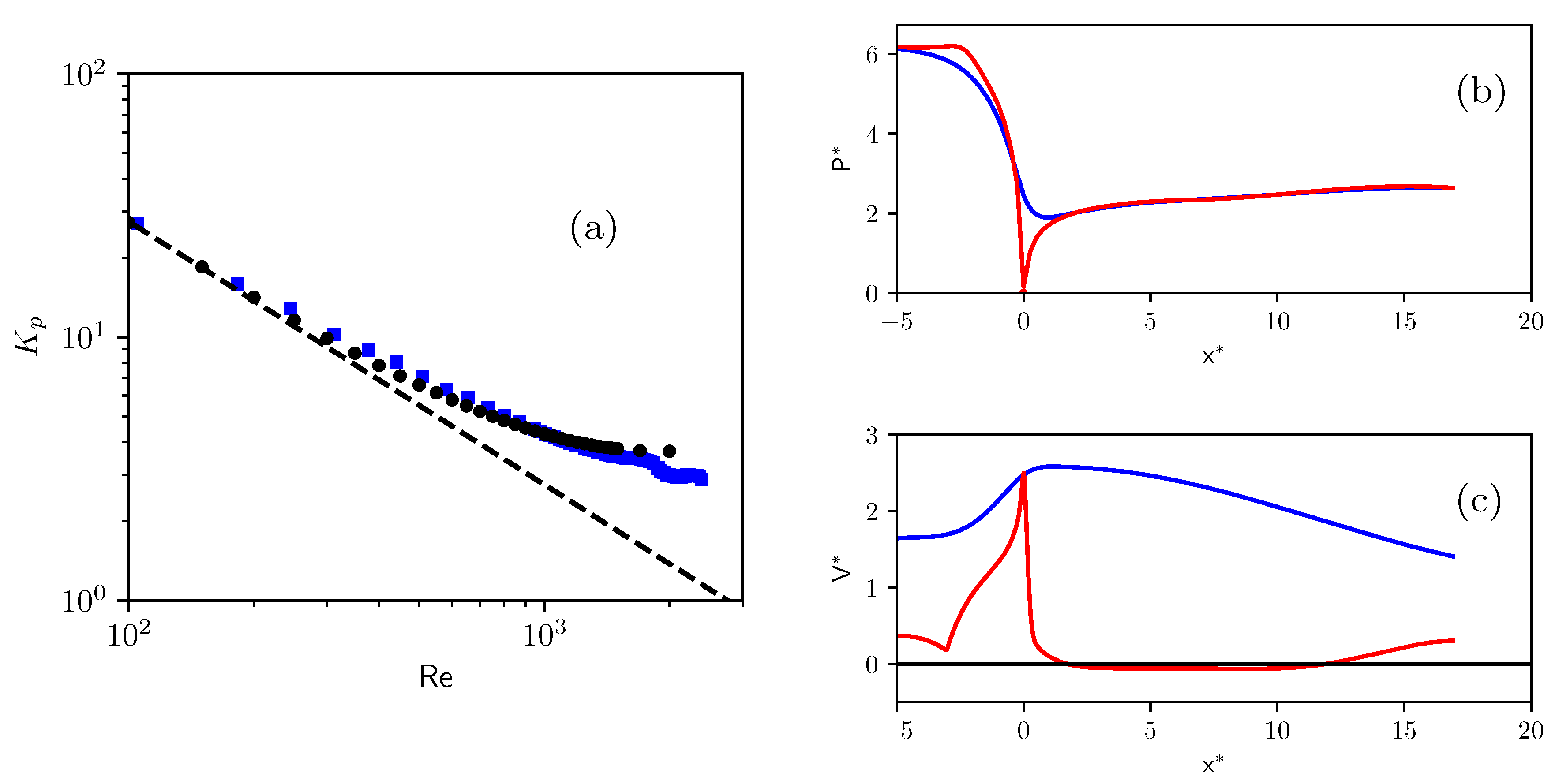
The topology of the single-phase flow and its nature as a function of the Reynolds number have been studied numerically [28]. The computation was performed with the Computational Fluid Dynamics code StarCCM+ (version 13.02). It uses a finite volume approach. The computation is three-dimensional; the numerical domain is similar to the experiment with an extrusion of upstream of the inlet of the test section and an extrusion of downstream of the outlet of the test section. The boundary conditions are a uniform inlet velocity and a uniform static pressure outlet. The domain is meshed with a structured grid. A grid convergence test was made at with up to cells. The final mesh contains cells, with 51 points in the cross-stream direction and a near-wall cell size of . The equations that are solved are the incompressible Navier–Stokes equations for a Newtonian fluid with constant properties. The spatial discretization for the convective flux is the second-order upwind scheme. Unsteady simulations with the Euler first-order implicit scheme have been performed. The main results are plotted in Figure 4. The experimental (obtained in single-phase flows) and numerical pressure loss coefficients fairly collapse, which is a clue in favor of the quality of the simulations (Figure 4a).
The main results of this numerical study are the following:
- The flow remains laminar for . A primary flow separation is present in the wake of the throat, on the divergent wall ( and ), first along each lateral wall () for , and on all along the width for . This corresponds to the negative values of the velocity profile in Figure 4c.
- A secondary laminar boundary layer separation emerges at a Reynolds number at the top wall of the test section ( and ).
- Finally, the critical cavitation numbers that lead to a minimal absolute pressure equal to the vapor pressure can be estimated numerically with the simulations. For instance, here, for , and , one can notice that the minimal pressure is close to zero and that this occurs at the throat, on the bottom wall (see Figure 4b). According to the simulation, cavitation of the oil is thus possible.
3. Results
3.1. Comparison between Degassed and Air-Saturated Oil
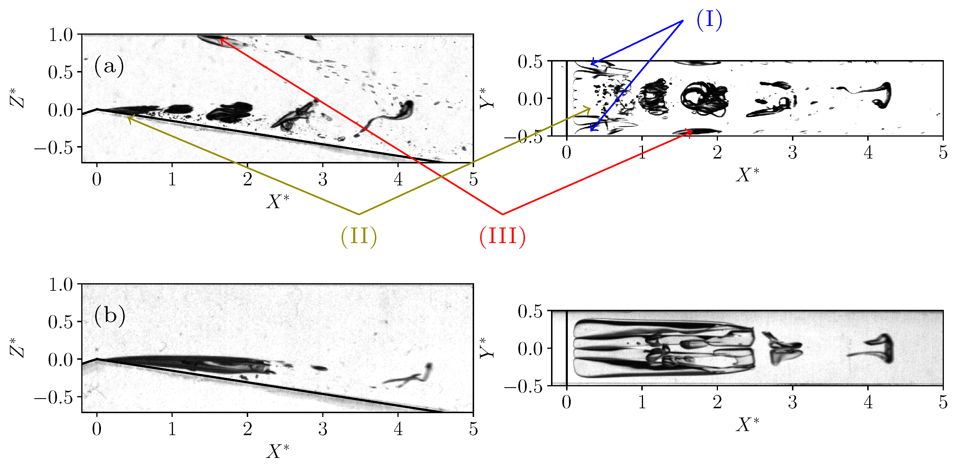
In the previous study using silicone oil saturated with air at 1 bar (Croci et al. (2019) [28]), three types of gaseous/vaporous structures have been observed. A typical example obtained at , and is shown in Figure 5a. The first one is called “bottom tadpoles” (see label (I) in Figure 5a). They attach to the side walls close to the throat, in the region of the primary flow separation that has been numerically demonstrated, and can be distinguished only in the top view. These structures appear for and at inlet pressures well above the estimated critical value for cavitation. They thus might be composed of degassed air. The second type of structure consists of an attached cavity in the middle of the vein, just downstream of the throat (see label (II) in Figure 5a). It has been observed for and their inception fairly corresponds to the critical value of the cavitation number estimated with numerical simulations. This attached cavity thus probably contains vapor. The third type of structures is reminiscent of the tadpoles and has been called “top tadpoles” (see label (III) in Figure 5a): they appear for and attach to the upper wall in the secondary boundary layer separation. The pressure in these regions is above the vapor pressure and they might also be composed of degassed air.
In the present article, with a different protocol of intense degassing at 70 mbars before running the experiments, the bottom and top tadpoles are not observed (see Figure 5b, obtained at , and ). This confirms that the top and bottom tadpoles are linked to degassing phenomena. Only the central attached cavity remains, and these cavities are moreover observed for cavitation numbers lower than the numerical critical value.
The following paragraphs are devoted to the study of the development of these cavities when varying the absolute pressure at constant Reynolds number.
3.2. Developed Cavitation Regimes Identification in Degassed Oil
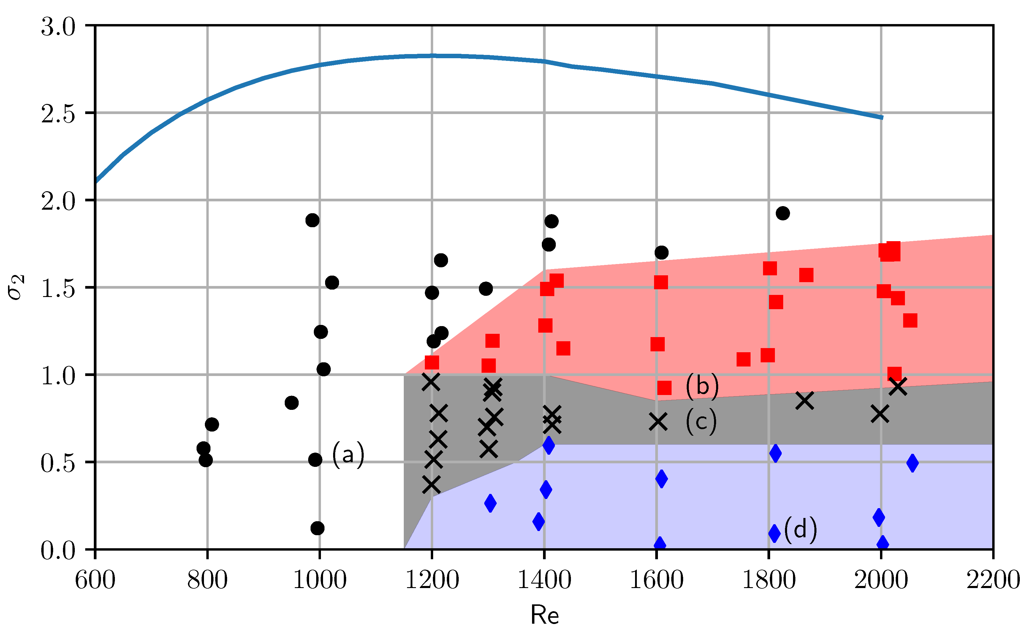
Approximately one hundred of movies have been recorded at various Reynolds numbers and cavitation numbers. Only the cases with no spurious air bubbles coming from upstream and with cavities larger than 1 mm have been reported in Figure 6.
The data all fall below the numerical inception curves. Four different regimes have been identified. Typical instantaneous side and top views illustrating these four regimes are displayed in Figure 7. The first regime identified with a full circle (•) corresponds to steady cavities. For , even at very small cavitation numbers, only steady cavities of this type are observed. The cavity viewed from side is quite flat and its bottom part is detached from the divergent bottom wall.
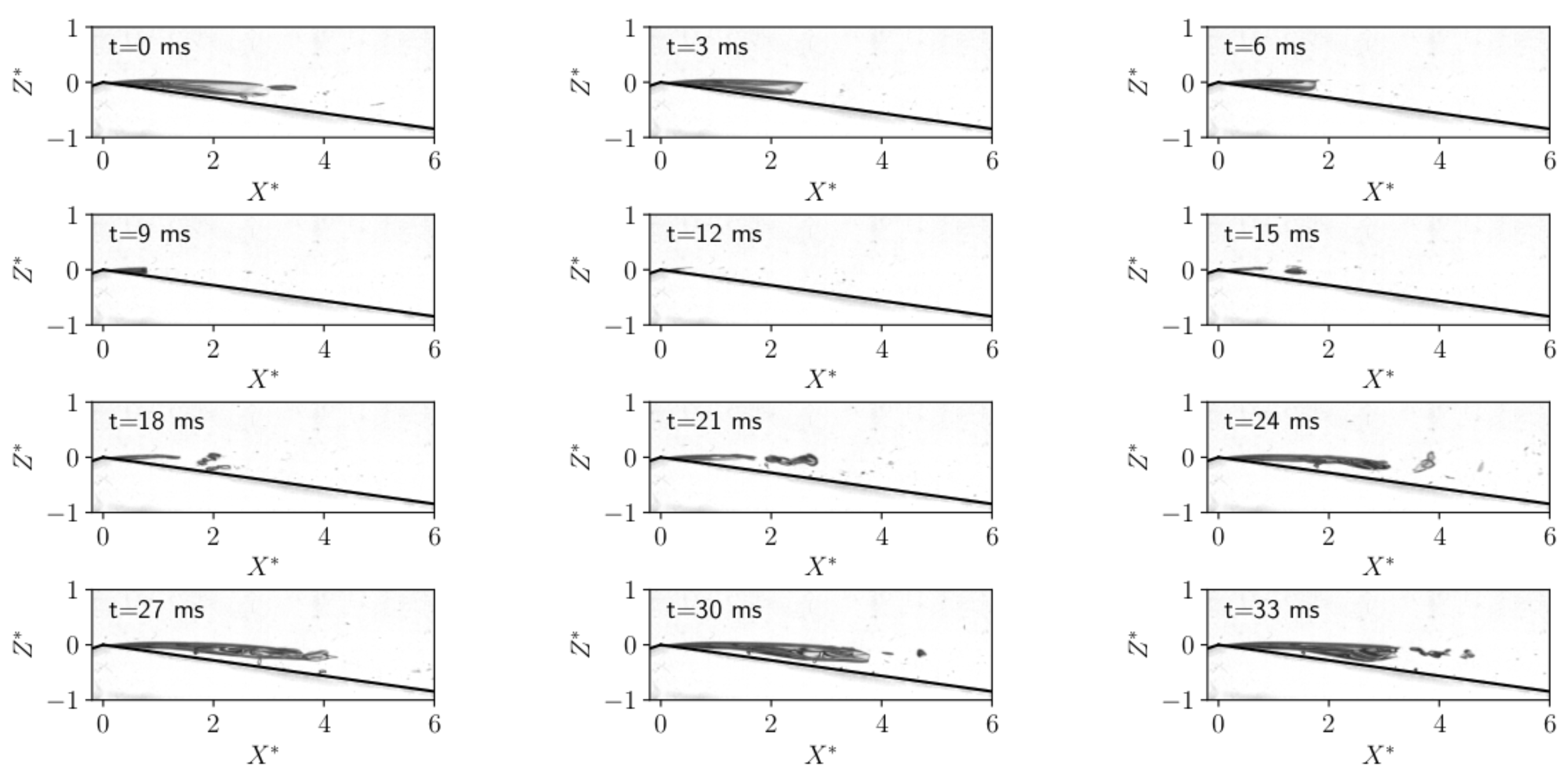
For larger Reynolds numbers (), the type-1 steady attached cavities are only observed at high cavitation numbers, corresponding to small cavities. When lowering the cavitation number, a second regime arises: the cavity periodically grows and shrinks, which corresponds to spatio-temporal diagrams looking like the one displayed in Figure 3c. A typical cycle of shrinking and growing is illustrated in Figure 8. This second regime, characterized by a “sawteeth” spatio-temporal diagram is called “type-2 cavities with periodic shrinking” and is displayed with red squares (▪). In this regime, the shape of the cavity is different and varies during the cycle. It consists of an elongated bubble with a narrow tail at maximum length and during the shrinking, one can observe that the tail of the cavity turns into a vertical front that collapses towards the throat. For the case illustrated in Figure 8, the length of the cavity varies between and .
Lowering further the cavitation number, the attached cavity loses this periodic behavior: the spatio-temporal diagrams still show unsteadiness in the flow but with no clear periodic cycle. This third regime is displayed with crosses (×) in Figure 6. The variation of its length corresponds this time to the detachment of delta and hairpin vortices as can be seen in Figure 7c. The cavity in this case keeps a length greater than and has a maximum length of the order of . The characteristic vertical front at the rear part of the cavity that has been noticed in the previous regime is no longer observed.
Finally, at the lowest cavitation numbers, one can obtain an almost steady cavity that appears to be completely transparent from both top and side view, and whose length is longer than the end of the divergent part of the Venturi profile (i.e., ). (see Figure 7d). This fourth type is called “supercavities” and is displayed with blue diamonds (⧫) in Figure 6.
3.3. Quantitative Characterization of the Different Regimes and Effects of the Reynolds Number
The type-2 cavities with periodic shrinking are first observed in a very narrow region of the parameter space for and are then present in a wider range of cavitation numbers for : they are found to lie in .
The type-4 supercavities have been observed only for one point at very low pressure at (). If supercavities exist for it would be at . However, for higher Reynolds numbers, i.e., for the zone where supercavities are observed progressively extends up to a constant value of the cavitation number .
There thus seems to be a progressive transition in the dynamics of attached sheet cavitation at very low Reynolds number between and . Quantitative measurements of the temporal and spatial features of the attached cavities are analyzed and discussed in the next paragraph.
First, the frequency of the periodic shrinking for all the type-2 cavities that have been identified (▪ in Figure 6) are plotted as a function of the throat velocity in Figure 9. The two quantities are highly correlated: the frequency seems to be proportional to the throat velocity, following a law . A Strouhal number based on the throat velocity and on the throat height as a length scale is . The type-2 regime is thus characterized by a constant Strouhal number of the order of . Such a low value is reminiscent of the “sheet cavity oscillation” regime described for a turbulent flow in a similar water experiment by Danlos et al. (2014) [10] as opposed to the “cloud cavitation” regime that is characterized by a Strouhal number greater by almost one order of magnitude. Moreover, in that study [10] the sheet cavity oscillation was observed to dominate the dynamics for short cavities and to disappear as the cavity length increases.
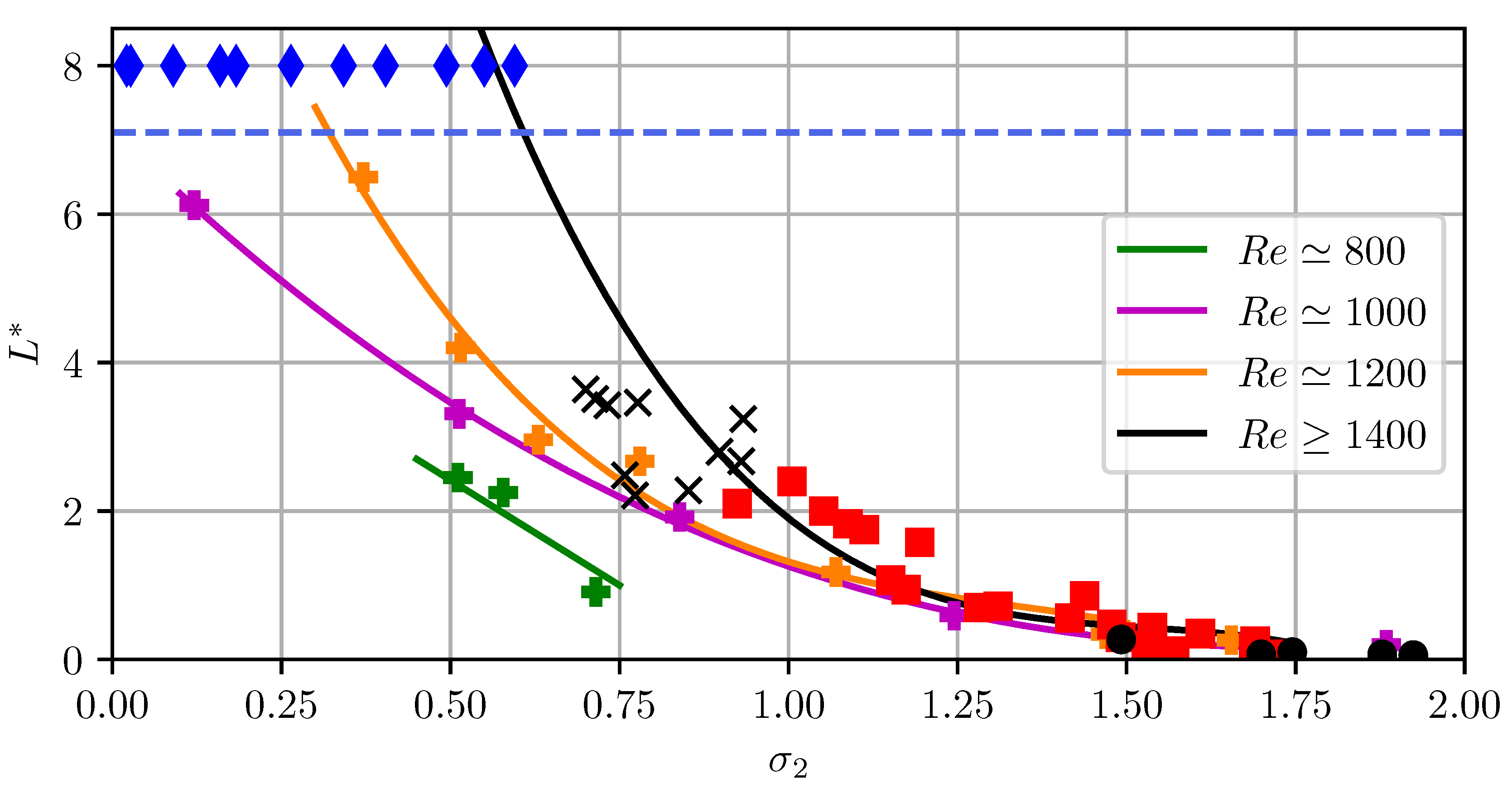
The evolution of the average length of the cavities as a function of the outlet cavitation number is plotted in Figure 10. For all Reynolds numbers, the overall trend is an increase of the length with a decrease of the cavitation number, which is not surprising. However, the shape of the curve exhibits a dependence on the Reynolds number. One can indeed notice that the curve becomes steeper as the Reynolds number increases, from to . At very low Reynolds number the cavity grows relatively slowly with a decrease of the cavitation number and the transition to super-cavitation is progressive at . The data obtained for then follow a different trend, with first a slow growing until and then a faster growing of the cavity. Moreover, one can notice that for , the transition between the type-2 regime (▪) and the type-3 regime (×) corresponds to an average length , around .
The dimensionless pressure drop in the experiment without cavitation, i.e., at , is plotted in Figure 4a as a function of the Reynolds number. Let us recall that . As the cavitation develops while decreasing the ambient pressure at constant discharge velocity, the presence of gaseous structures of increasing volume may change the pressure drop. It might thus be interesting to explore the variation of both the inlet and outlet pressure, i.e., in a dimensionless form of both and . The experiments are plotted in this parameter space in Figure 11. The points at constant Reynolds number are plotted with the same symbol.
The development of cavitation associated with a decrease of the ambient pressure corresponds to a path from top right to bottom left in this parameter space. For the seven Reynolds numbers that are displayed in the Figure 11, one can first notice that the points follow a similar trend: the two pressures are decreasing together. Moreover, one can distinguish two main different shapes in the curves. On the one hand, for and , the points align quite on a straight path. On the other hand, for , one can notice some kind of break in the slope of the curve around . For , the slope is of the order of magnitude of the former (roughly ), whereas for , the slope is steeper, of the order of : a very small decrease in the inlet pressure causes a dramatic decrease of the outlet pressure corresponding to the fast increase of the cavity length observed in Figure 10.
These observations support the idea of a transition in the cavitating flow that takes place around .
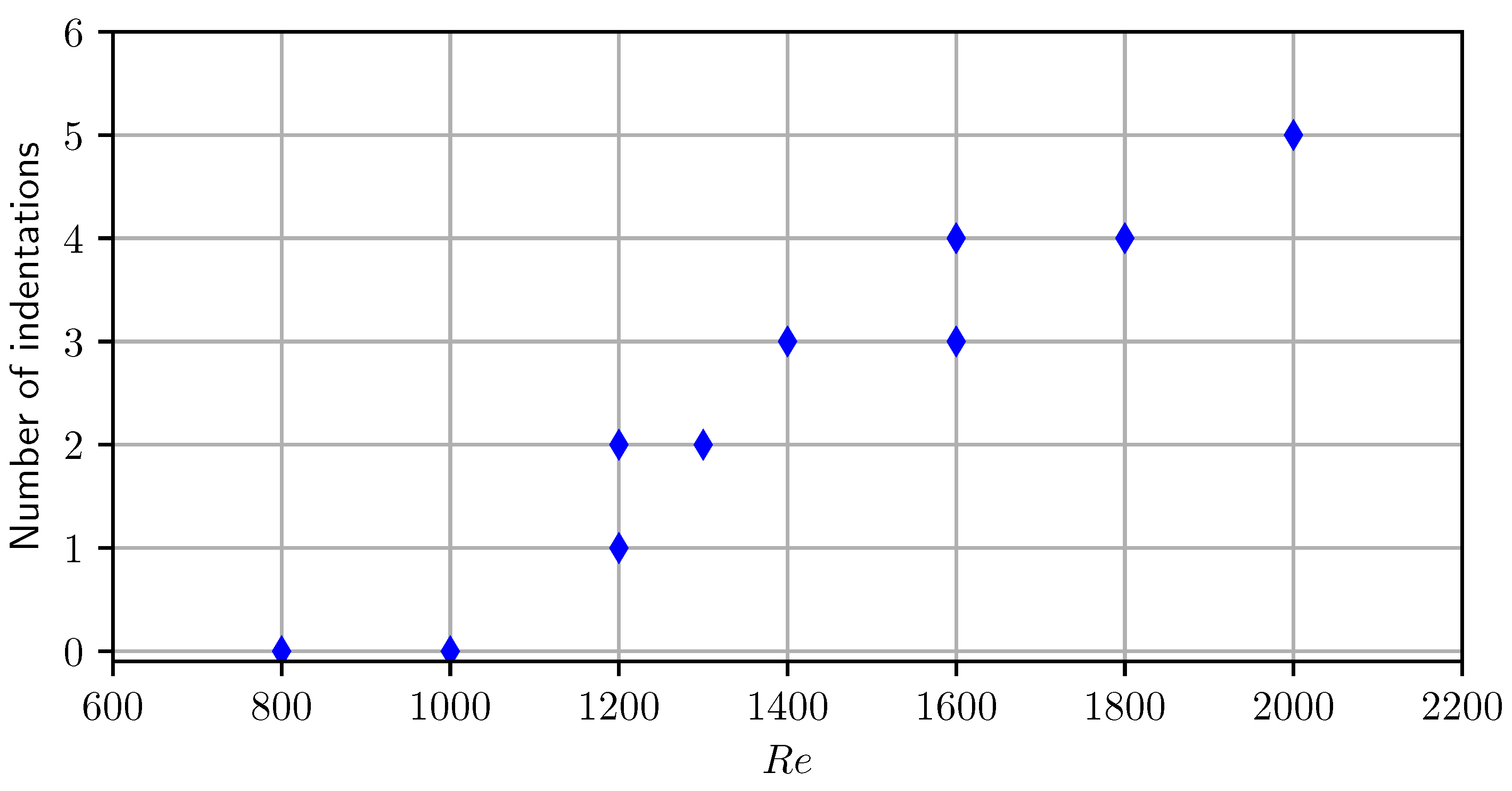
Looking at the attached cavities from top (see the right column in Figure 2, Figure 5 and Figure 7), one can notice that the morphology of the cavity also exhibits a dependence in the transverse direction . At very low Reynolds number (see Figure 7a) the interface at the leading edge presents a single smooth and convex cap. At larger Reynolds numbers (see Figure 7d) this interface presents several indentations. These structures resemble the “divots” that have been discussed for instance in Ref. [35] and that are attributed to a local breakdown of the two-dimensionality of the laminar boundary layer. We report in Figure 12 the number of indentations that are observed on the cavities of an average length of . The first indentation is observed at and then their number increases almost linearly with the Reynolds number.
4. Conclusions
In the present article, the development of attached cavities under cavitating conditions in a highly degassed silicone oil has been explored, at Reynolds numbers in the range . The regime map in terms of Reynolds and cavitation numbers have been established. Four different regimes have been observed: type-1 small cavities that are almost steady, type-2 periodically shrinking cavities of intermediate sizes, type-3 vortex bursting with no clear period and type-4 supercavities. For , the background flow is steady and laminar and the cavitating flow gives rise to steady attached cavities whose length slowly increases with a decrease of the cavitation number. The first footprint of unsteadiness in the cavitating flow consists of the type-2 periodic regime. It appears for a sufficiently great Reynolds number (), first in a very narrow range of cavitation numbers and then in a wider range as . The frequency is almost proportional to the velocity of the upstream flow and gives a constant Strouhal number of very small value. More modal analysis with POD (Proper Orthogonal Decomposition) or DMD (Dynamic Mode Decomposition) is in progress to characterize better this regime. These experiments will require higher temporal resolution. The analysis of the length of the cavity, of the transition to super-cavitation and of the evolution of the pressure drop are consistent with a smooth transition in the cavitating flow for , which corresponds to the range where the single-phase (non-cavitating) flow is transitional. It would be interesting to extend further the range of Reynolds numbers, using an oil of lower viscosity, in order to give a lower bound in Reynolds number for the periodical cloud shedding regime that is known to take place in this geometry in fully developed turbulent flows.
Author Contributions
Conceptualization, F.R., F.B., A.D. and S.K.; methodology, F.R.; software, F.R.; validation, F.R., F.B., A.D. and S.K.; formal analysis, F.R.; investigation, F.R. and A.D; resources, K.C. and C.S.; data curation, F.R. and A.D.; writing–original draft preparation, F.R.; writing–review and editing, F.R.; visualization, F.R.; supervision, F.B. and S.K.; project administration, F.R.; funding acquisition, F.B. and S.K. All authors have read and agreed to the published version of the manuscript.
Funding
This research received no external funding.
Acknowledgments
The authors acknowledge Marc Joulin and Jocelyn Mistigres for technical support, and Michaël Pereira for fruitful discussion.
Conflicts of Interest
The authors declare no conflict of interest.
References
- Brennen, C.E. Fundamentals of Multiphase Flows; Cambridge University Press: Cambridge, England, 2005. [Google Scholar]
- Franc, J.P.; Michel, J.M. Fundamentals of Cavitation; Kluwer Academic Publishers: Dordrecht, The Netherlands, 2006. [Google Scholar]
- Parkin, B.R.; Kermeen, R.W. Incipient Cavitation and Boundary Layer Interaction on a Streamlined Body; Rep. E-35.2; California Institute of Technology: Pasadena, CA, USA, 1953. [Google Scholar]
- Arakeri, V.H. Viscous effects on the position of cavitation separation from smooth bodies. J. Fluid Mech. 1975, 68, 779–799. [Google Scholar] [CrossRef] [Green Version]
- Kuiper, G. Cavitation Inception on Ship Propeller Models. Ph.D. Thesis, Delft University of Technology, Delft, The Netherlands, 1981. [Google Scholar]
- Franc, J.P.; Michel, J.M. Attached cavitation and the boundary layer: Experimental investigation and numerical treatment. J. Fluid Mech. 1985, 154, 63–90. [Google Scholar] [CrossRef]
- Guennoun, M.F. Étude Physique de Lapparition et du D’veloppement de la Cavitation sur une aube Isolée. Ph.D. Thesis, EPFL Lausanne, Lausanne, Switzerland, 2006. [Google Scholar]
- van Rijsbergen, M. A review of sheet cavitation inception mechanisms. In Proceedings of the 16th International Symposium on Transport Phenomena and Dynamics of Rotating Machinery, Honolulu, HI, USA, 10–15 April 2016; Available online: https://hal.archives-ouvertes.fr/hal-01890067/ (accessed on 10 October 2020).
- Brandner, P.; Walker, G.J.; Niekamp, P.N.; Anderson, B. An experimental investigation of cloud cavitation about a sphere. J. Fluid Mech. 2010, 656, 147–176. [Google Scholar] [CrossRef]
- Danlos, A.; Ravelet, F.; Coutier-Delgosha, O.; Bakir, F. Cavitation regime detection through Proper Orthogonal Decomposition: Dynamics analysis of the sheet cavity on a grooved convergent divergent nozzle. Int. J. Heat Fluid Flow 2014, 47, 9–20. [Google Scholar] [CrossRef] [Green Version]
- Pelz, P.F.; Keil, T.; Groß, T.F. The transition from sheet to cloud cavitation. J. Fluid Mech. 2017, 817, 439–454. [Google Scholar] [CrossRef] [Green Version]
- Šarc, A.; Kosel, J.; Stopar, D.; Oder, M.; Dular, M. Removal of bacteria Legionella pneumophila, Escherichia coli, and Bacillus subtilis by (super)cavitation. Ultrason. Sonochem. 2018, 42, 228–236. [Google Scholar] [CrossRef]
- Kosel, J.; Šuštaršič, M.; Petkovšek, M.; Zupanc, M.; Sežun, M.; Dular, M. Application of (super)cavitation for the recycling of process waters in paper producing industry. Ultrason. Sonochem. 2020, 64, 10500. [Google Scholar] [CrossRef]
- Tsujimoto, Y.; Kenjiro, K.K.; Brennen, C.E. Unified treatment of flow instabilities of turbomachines. J. Propuls. Power 2001, 17, 636–643. [Google Scholar] [CrossRef]
- Campos-Amezcua, R.; Bakir, F.; Campos-Amezcua, A.; Khelladi, S.; Palacios-Gallegos, M.; Rey, R. Numerical analysis of unsteady cavitating flow in an axial inducer. Appl. Therm. Eng. 2015, 75, 1302–1310. [Google Scholar] [CrossRef] [Green Version]
- Callenaere, M.; Franc, J.P.; Michel, J.M.; Riondet, M. The cavitation instability induced by the development of a re-entrant jet. J. Fluid Mech. 2001, 444, 223–256. [Google Scholar] [CrossRef]
- Ganesh, H.; Mäkiharju, S.A.; Ceccio, S.L. Bubbly shock propagation as a mechanism for sheet-to-cloud transition of partial cavities. Phys. Fluids 2016, 802, 37–78. [Google Scholar] [CrossRef] [Green Version]
- Croci, K.; Tomov, P.; Ravelet, F.; Danlos, A.; Khelladi, S.; Robinet, J.C. Investigation of two mechanisms governing cloud cavitation shedding: Experimental study and numerical highlight. In Proceedings of the ASME International Mechanical Engineering Congress and Exposition, Phoenix, AZ, USA, 11–17 November 2016; Volume 7. [Google Scholar]
- Wu, J.; Ganesh, H.; Ceccio, S. Multimodal partial cavity shedding on a two-dimensional hydrofoil and its relation to the presence of bubbly shocks. Exp. Fluids 2019, 60, 66. [Google Scholar] [CrossRef]
- Brunhart, M.; Soteriou, C.; Gavaises, M.; Karathanassis, I.; Koukouvinis, P.; Jahangir, S.; Poelma, C. Investigation of cavitation and vapor shedding mechanisms in a Venturi nozzle. Phys. Fluids 2020, 32, 083306. [Google Scholar] [CrossRef]
- Petkovšek, M.; Hocevar, M.; Dular, M. Visualization and measurements of shock waves in cavitating flow. Exp. Therm. Fluid Sci. 2020, 119, 110215. [Google Scholar] [CrossRef]
- Trummler, T.; Schmidt, S.; Adams, N. Investigation of condensation shocks and re-entrant jet dynamics in a cavitating nozzle flow by Large-Eddy Simulation. Int. J. Multiph. Flow 2020, 125, 103215. [Google Scholar] [CrossRef] [Green Version]
- Ishihara, T.; Ouchi, M.; Kobayashi, T.; Tamura, N. An experimental study on cavitation in unsteady oil flow. Bull. JSME 1979, 22, 1099–1106. [Google Scholar] [CrossRef]
- Washio, S.; Kikui, S.; Takahashi, S. Nucleation and subsequent cavitation in a hydraulic oil poppet valve. Proc. Inst. Mech. Eng. Part C J. Mech. Eng. Sci. 2009, 224, 947–958. [Google Scholar] [CrossRef]
- Peters, F.; Honza, R. A benchmark experiment on gas cavitation. Exp. Fluids 2014, 55, 1786. [Google Scholar] [CrossRef]
- Groß, T.F.; Pelz, P.F. Diffusion-driven nucleation from surface nuclei in hydrodynamic cavitation. J. Fluid Mech. 2017, 830, 138–164. [Google Scholar] [CrossRef] [Green Version]
- Croci, K.; Ravelet, F.; Robinet, J.C.; Danlos, A. Experimental Study of Cavitation in Laminar Flow. In Proceedings of the 10th International Symposium on Cavitation (CAV2018), Baltimore, MD, USA, 14–16 May 2018. [Google Scholar] [CrossRef] [Green Version]
- Croci, K.; Ravelet, F.; Danlos, A.; Robinet, J.C.; Barast, L. Attached cavitation in laminar separations within a transition to unsteadiness. Phys. Fluids 2019, 31, 063605. [Google Scholar] [CrossRef] [Green Version]
- Ding, C.; Fan, Y. Measurement of diffusion coefficients of air in silicone oil and in hydraulic oil. Chin. J. Chem. Eng. 2011, 19, 205–211. [Google Scholar] [CrossRef]
- Li, B.; Gu, Y.; Chen, M. An experimental study on the cavitation of water with dissolved gases. Exp. Fluids 2017, 58, 164. [Google Scholar] [CrossRef]
- Amini, A.; Reclari, M.; Sano, T.; Farhat, M. Effect of gas content on tip vortex cavitation. In Proceedings of the Symposium on Cavitation, Baltimore, MD, USA, 14–16 May 2018. [Google Scholar]
- Croci, K. Experimental Study of Multiphase Flows within a Separated Laminar Boundary Layer. Ph.D. Thesis, Ecole Nationale Supérieure D’arts et métiers—ENSAM, Paris, France, 2018. [Google Scholar]
- van der Walt, S.; Schönberger, J.L.; Nunez-Iglesias, J.; Boulogne, F.; Warner, J.D.; Yager, N.; Gouillart, E.; Yu, T.; the scikit-image contributors. scikit-image: Image processing in Python. PeerJ 2014, 2, e453. [Google Scholar] [CrossRef] [PubMed]
- Soille, P. Morphological Image Analysis; Springer: Berlin, Germany, 2004. [Google Scholar]
- Tassin Leger, A.; Bernal, L.P.; Ceccio, S.L. Examination of the flow near the leading edge of attached cavitation. Part 2. Incipient breakdown of two-dimensional and axisymmetric cavities. J. Fluid Mech. 1998, 376, 91–113. [Google Scholar] [CrossRef]
Figure 1.
Sketch of the Venturi geometry. The width of the test section is mm and its height at the inlet section is mm. In the following of the article the axes origin is positioned at the Venturi throat edge in the middle of test section along the width. Reprinted with permission from K. Croci, Ph.D. dissertation [32].

Figure 2.
(a) Typical side (left column) and top (right column) instantaneous views. The flow is from left to right. , and . (b) Illustration of the image processing. The treatment is based on binarization, morphological closing and regions labeling (see text for details). The large region close to the throat is displayed in black in the figure, whereas the other small gaseous cavities are in white and the background in pale gray. A binary image (not shown) is generated that only contain the large region close to the throat. (c) Time average of 3000 binary images showing the average attached cavity on the side and top views. The colorbar corresponds to the proportion of time when the cavity is present.

Figure 3.
Illustration of image processing for the characterization of the temporal features of the attached cavities. (a): Instantaneous normalized side view at , and . (b): Gray level along the dashed blue line displayed in (a); is the dimensionless curvilinear abscissa along the line. (c): Spatio-temporal diagram along the line; space is from top to bottom and time is from left to right. (d): Corresponding temporal magnitude spectrum.

Figure 4.
Main results of the single-phase numerical simulations. (a) Pressure loss coefficient as a function of the Reynolds number . Blue squares represent experimental values while black squares represent numerical simulations. The dashed line is a line of equation . (b) Dimensionless pressure profile with respect to axial coordinate . (c) Dimensionless velocity profile with respect to . For both images (b,c): , and ; Blue line is along the horizontal line and ; Red line is a broken line following the bottom of the vein, mm above it at .

Figure 5.
Comparison between two experiments performed at similar Reynolds numbers () and cavitation numbers () with a different degassing protocol. (a): Silicone oil is saturated with air at 1 bar before running the experiment. The three types of gaseous structures are spotted with (I) for bottom tadpoles, (II) for attached sheet cavity and (III) for top tadpoles. (b): Silicone oil is first degassed at 70 mbars; an attached sheet cavity is only present.

Figure 6.
Explored map in the Reynolds—cavitation number () space. Black circles (•) correspond to type-1 steady small cavities, red squares (▪) to type-2 cavities with periodic shrinking, crosses (×) to type-3 unsteady cavities with no clear periodic behavior and blue diamonds (⧫) to type-4 supercavities with . The solid pale blue line corresponds to the critical cavitation numbers obtained with the single-phase numerical simulations. Images of the cases (a) to (d) are displayed in Figure 7.

Figure 7.
Side and top views in different regimes. (a): type-1 steady cavity (•) at , and . (b): type-2 cavity with periodic shrinking (▪) at , and . (c): type-3 unsteady cavity with no clear periodic behavior (×) at , and . (d): to type-4 supercavity (⧫) at , and .
Figure 7.
Side and top views in different regimes. (a): type-1 steady cavity (•) at , and . (b): type-2 cavity with periodic shrinking (▪) at , and . (c): type-3 unsteady cavity with no clear periodic behavior (×) at , and . (d): to type-4 supercavity (⧫) at , and .

Figure 8.
One cycle viewed from side in the type-2 periodic shrinking regime (▪) at , and . The measured frequency of the cycle is .
Figure 8.
One cycle viewed from side in the type-2 periodic shrinking regime (▪) at , and . The measured frequency of the cycle is .

Figure 9.
Measured frequency as a function of the throat velocity for type-2 regime. The dashed line is a linear fit of equation .
Figure 9.
Measured frequency as a function of the throat velocity for type-2 regime. The dashed line is a linear fit of equation .

Figure 10.
Dimensionless average length of the attached cavity as a function of the outlet cavitation number . For , the symbols refer to the regimes identified in Figure 6: type-1 steady cavity (•), type-2 cavity with periodic shrinking (▪), type-3 unsteady cavity with no clear periodic behavior (×) and type-4 supercavity (⧫). The lines are a guide to the eye based on spline interpolation of the points at , , and of all the points for .

Figure 11.
Explored map in the inlet cavitation number—outlet cavitation number (). The different symbols stand for different Reynolds numbers. The arrows are guides to the eye.
Figure 11.
Explored map in the inlet cavitation number—outlet cavitation number (). The different symbols stand for different Reynolds numbers. The arrows are guides to the eye.

Figure 12.
Number of transverse indentations at the leading edge of the developed attached cavities as a function of the Reynolds number.
Figure 12.
Number of transverse indentations at the leading edge of the developed attached cavities as a function of the Reynolds number.


Table 1.
Flow parameters, ranges and estimated uncertainties for silicone oil . The surface tension is mN·m and the vapor pressure is Pa according to the oil data file.
Table 1.
Flow parameters, ranges and estimated uncertainties for silicone oil . The surface tension is mN·m and the vapor pressure is Pa according to the oil data file.
| Symbol | Parameters | Definition | Range | Unit | Uncertainty |
|---|---|---|---|---|---|
| Inlet pressure | mbar | ||||
| Outlet pressure | mbar | ||||
| T | Operating temperature | C | |||
| Inlet velocity | m·s | ||||
| Oil density | kg·m | ||||
| Oil kinematic viscosity | mm·s | ||||
| Capillary number | ⩽3% | ||||
| Pressure loss coefficient | ⩽4% | ||||
| Inlet Reynolds number | ⩽3% | ||||
| Inlet cavitation number | ⩽2% | ||||
| Outlet cavitation number | ⩽2% |
Publisher’s Note: MDPI stays neutral with regard to jurisdictional claims in published maps and institutional affiliations. |
© 2020 by the authors. Licensee MDPI, Basel, Switzerland. This article is an open access article distributed under the terms and conditions of the Creative Commons Attribution (CC BY) license (http://creativecommons.org/licenses/by/4.0/).
Share and Cite
MDPI and ACS Style
Ravelet, F.; Danlos, A.; Bakir, F.; Croci, K.; Khelladi, S.; Sarraf, C. Development of Attached Cavitation at Very Low Reynolds Numbers from Partial to Super-Cavitation. Appl. Sci. 2020, 10, 7350. https://doi.org/10.3390/app10207350
AMA Style
Ravelet F, Danlos A, Bakir F, Croci K, Khelladi S, Sarraf C. Development of Attached Cavitation at Very Low Reynolds Numbers from Partial to Super-Cavitation. Applied Sciences. 2020; 10(20):7350. https://doi.org/10.3390/app10207350
Chicago/Turabian StyleRavelet, Florent, Amélie Danlos, Farid Bakir, Kilian Croci, Sofiane Khelladi, and Christophe Sarraf. 2020. "Development of Attached Cavitation at Very Low Reynolds Numbers from Partial to Super-Cavitation" Applied Sciences 10, no. 20: 7350. https://doi.org/10.3390/app10207350
Note that from the first issue of 2016, this journal uses article numbers instead of page numbers. See further details here.