Simulation of Water-Use Efficiency of Crops under Different Irrigation Strategies

Abstract

Irrigation management is a key factor in attaining optimal yields, as different irrigation strategies lead to different yields even when using the same amount of water or under the same weather conditions. Our research aimed to simulate the water-use efficiency (WUE) of crops considering different irrigation strategies in the Central Valley of Chile. By means of AquaCrop-OS, we simulated expected yields for combinations of crops (maize, sugar beet, wheat), soil (clay loam, loam, silty clay loam, and silty loam), and bulk density. Thus, we tested four watering strategies: rainfed, soil moisture-based irrigation, irrigation with a fixed interval every 1, 3, 5, and 7 days, and an algorithm for optimal irrigation scheduling under water supply constraints (GET-OPTIS). The results showed that an efficient irrigation strategy must account for soil and crop characteristics. Among the tested strategies, GET-OPTIS led to the best performance for crop yield, water use, water-use efficiency, and profit, followed by the soil moisture-based strategy. Thus, soil type has an important influence on the yield and performance of different irrigation strategies, as it provides a significant storage and buffer for plants, making it possible to produce “more crop per drop”. This work can serve as a methodological guide for simulating the water-use efficiency of crops and can be used alongside evidence from the field.

1. Introduction

Irrigation and irrigation management are the main factors that affect crop yields and water use by making crop development independent from rainfall. However, poor irrigation management can lead to several in-farm and off-farm impacts, such as waterlogging, changes in river flows, erosion and nonpoint pollution [1]. Improving irrigation management increases water-use efficiency (WUE), i.e., the ratio of applied water to crop yield, by decreasing the amount of water necessary to achieve a given production or increasing yields. According to the Food and Agriculture Organization of the United Nations (FAO) [2], agriculture uses ca. 70% of the available freshwater. Therefore, increasing water-use efficiency will allow us to decrease the amount of water used in attaining expected yields [3]. However, the success of irrigation largely relies on proper management and the appropriate selection of irrigation strategies.

Implementing successful irrigation and water management strategies requires knowledge of several physical and empirical aspects of the system [4]. Field experiments are costly and resource consuming [5], and different soil tests and resource management strategies are required in order to obtain the best strategies by heuristic to fit specific cases.

Outputs from simulation models allow different irrigation strategies, soil and crop conditions, and changes in climatic conditions to be tested. AquaCrop [6] is a model that simulates yields dependant on irrigation strategies, climate, field management (soil fertility and field agronomic practices), soil profile, and the presence of groundwater. AquaCrop is able to simulate yields for maize [7,8,9], wheat [10,11,12], sugar beet [5,13,14], potatoes [15,16], barley [17], quinoa [18], and rice [19]. Foster et al. [20] developed the AquaCrop-OS model, an open source code written in MATLAB, which provides the opportunity to incorporate other concepts to assess farming scenarios.

Agricultural production and benefits largely rely on management, i.e., the set of rules and practices followed by farmers to irrigate, fertilize, and harvest crops. Thus, there are several ways to attain a given yield, such as through the irrigation schedule, monitoring systems, precision agriculture, among others. Thus, different farming strategies could give similar yields but produce different impacts on profit and the environment. Therefore, it is plausible to apply standardized methods to compare prediction strategies, considering economic, environmental, and social dimensions. Water-use efficiency (WUE) is a ratio that relates the yield to the water consumed by crops [21]. WUE has been used for maize [22,23], sugar beet [24,25], wheat [12,26], and other crops.

In this paper, we compare different irrigation strategies for a set of plausible combinations of crop, soil, and climate in Central Chile, by means of the WUE values derived from AquaCrop simulations. This methodology aids decision-making processes by presenting estimates of the impact of a given or in-use irrigation strategy. It also provides a heuristic to identify better strategies. Once the best strategy is set, it is possible to identify hardware and software gaps. Thus, this method should be seen as a support for decision-making rather than a method for obtaining precise yield estimates.

2. Methodology

The proposed methodology aims to compare different irrigation strategies using AquaCrop-OS to determine dry yield, water use, and WUE for different crops, considering local soils, weather conditions, sowing dates, and field management practices.

2.1. Water-Use Efficiency

Water-use efficiency (kg m⁻³) is an indicator related to the water consumed by crops (as evapotranspiration) to produce a certain yield [21]:

$$WUE=\left({\displaystyle \frac{Y}{ETa}}\right)\times 100$$

(1)

where Y and $ETa$ are crop yield (in t ha⁻¹) and actual evapotranspiration (in mm), respectively.

2.2. Irrigation Management

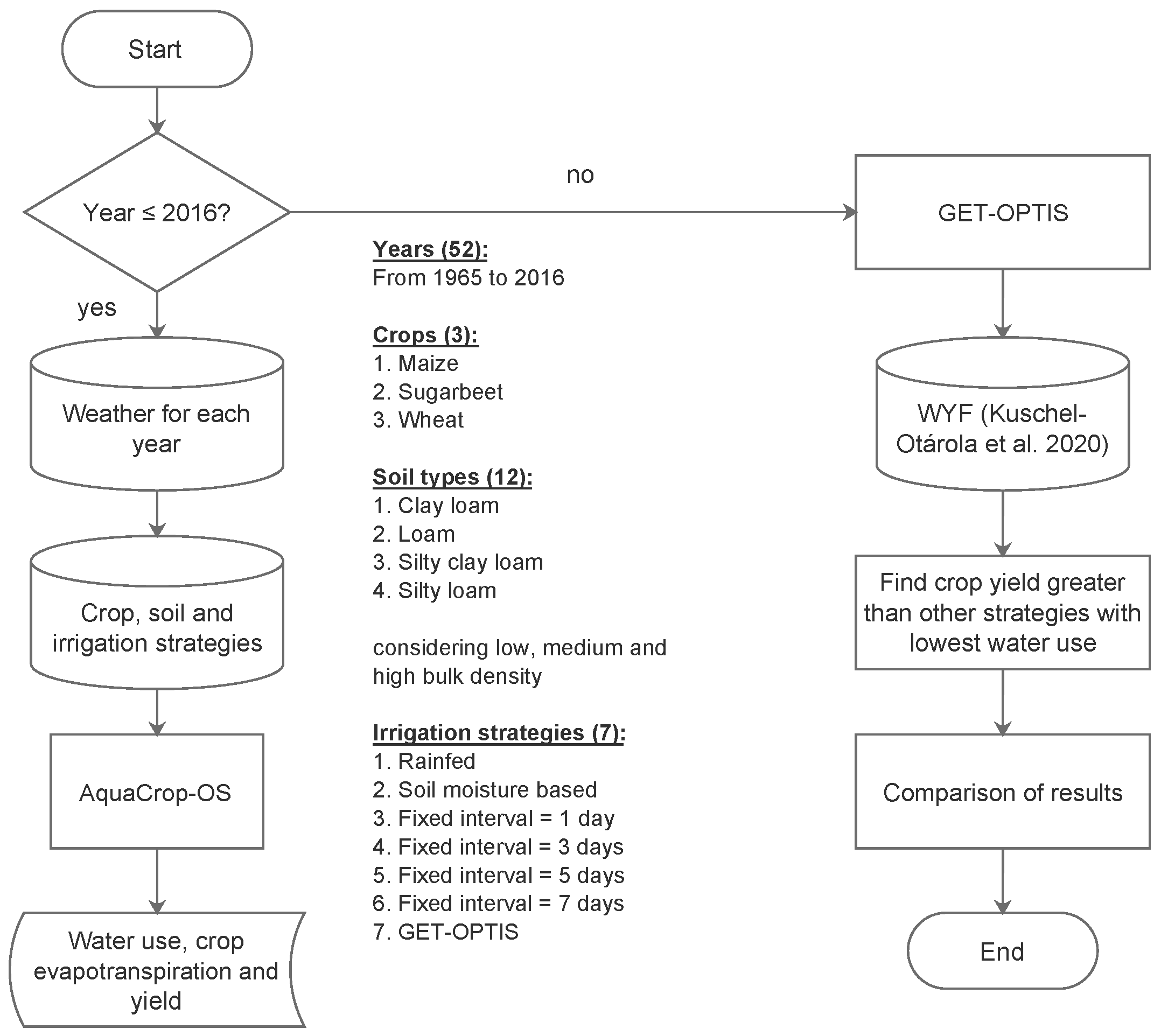
We compared water use, yield, and WUE for four different irrigation strategies: rainfed (no irrigation), soil moisture-based, a fixed interval irrigation every 1, 3, 5, and 7 days, and the optimal schedule for 52 years (

Table 1. Considered irrigation strategies.

Irrigation Strategy	Acronym	Criteria
Rainfed	RF	Crop water demands are satisfied only by rainfall.
Soil moisture-based	SMB	Crop is irrigated to field capacity (FC) when soil water content (SWC) reaches a threshold.
Fixed interval every 1 day	FI-1	Crop is always irrigated every day to FC. SWC target does not necessarily reach a threshold.
Fixed interval every 3 days	FI-3	Crop is always irrigated every 3 days to FC. SWC target does not necessarily reach threshold.
Fixed interval every 5 days	FI-5	Crop is always irrigated every 5 days to FC. SWC target does not necessarily reach threshold.
Fixed interval every 7 days	FI-7	Crop is always irrigated every 7 days to FC. SWC target does not necessarily reach threshold.
GET-OPTIS	G-O	Crop is irrigated following an optimal schedule. i.e., date and an irrigation depth (not necessarily to FC).

). We implemented a routine that feeds AquaCrop-OS [20] with daily weather data from 1965 to 2016 for maize, sugar beet, and wheat. We tested 12 combinations of soil type and bulk density.

To define the optimal schedule (S), i.e., the date ($d_i$) and amount of water for irrigation ($v_i$) leading to the highest yield (Y) for a given amount of available water, we used the Global Evolutionary Technique for OPTimal Irrigation Scheduling (GET-OPTIS) [27] to estimate the Water Yield Functions (WYF):

$$\begin{array}{cc}\hfill Y^{*}& =maxY\left(S\right):S={\left\{s_i\right\}}_{i=1,\dots ,n}\hfill \\ \hfill & =\left\{\left(d_1,v_1\right),\dots ,\left(d_i,v_i\right),\dots ,\left(d_n,v_n\right)\right\}n,d_i\in \mathbb{N};v_i\in \mathbb{R}\hfill \end{array}$$

(2)

Once WYF were built, we found the irrigation strategies with the greatest crop yield (rainfed, soil moisture-based, and fixed interval) and the lowest water use. Figure 1 summarizes the aforementioned methodology.

2.3. A Proxy for Economic Performance

A complete economic analysis requires a number of parameters and decisions made by farmers within the season. Even though detailed economical issues are out of the scope of this paper, we used the difference between income and irrigation costs as a proxy for economic performance (U in USD ha⁻¹):

$$U_{i,j,k}=P_i\times F_i\times Y_{i,j,k}-C\times W_{i,j,k}$$

(3)

where $P_i$ is the price per crop i (in USD t⁻¹), $F_i$ is a correction factor for yield for crop i (dimensionless), $Y_{i,j,k}$ corresponds to the crop yield (in t ha⁻¹) for crop i, soil type j, and irrigation strategy k. On the other hand, C is the irrigation cost (in USD mm⁻¹ ha⁻¹) and $W_{i,j,k}$ is the water use for crop i, soil type j, and irrigation strategy k. Regarding price per crop $P_i$, we considered values of 231.03, 47.00, and 167.41 (USD t⁻¹) for maize, sugar beet, and wheat, respectively, considering prices for the Chilean market. As AquaCrop-OS determines crop yield as dry yield, we considered that maize and wheat were harvested with a 14% moisture content. Therefore, the correction factor $F_i$ for those crops is 1.14. On the other hand, sugar beet stores sucrose in the tap root, so a 14–20% sucrose content $F_i$ is equal to 7.14 [28,29]. Regarding irrigation costs, we considered a mean value of 0.25 (USD mm⁻¹ ha⁻¹) using a center pivot irrigation system with an irrigation efficiency of 85% as a benchmark.

2.4. Application to Representative Conditions in Central Chile

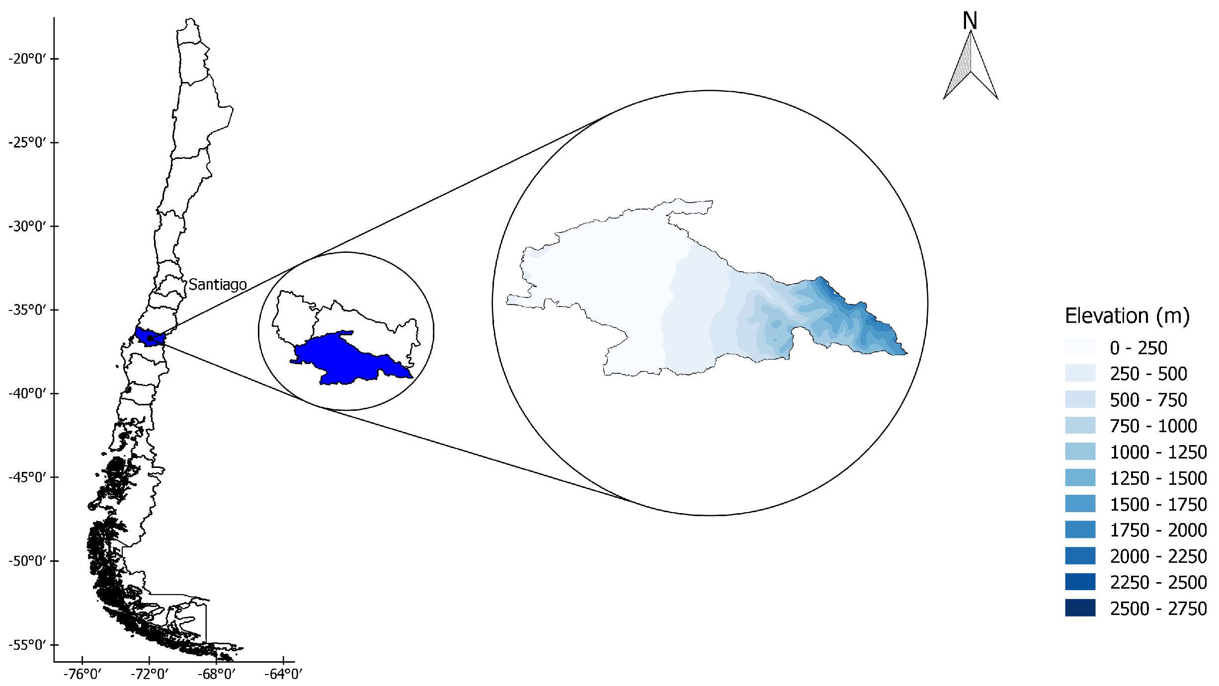
We used data and information for representative conditions of the Central Valley of Chile (Figure 2) to feed AquaCrop and subsequently obtain yield estimates. The annual precipitation is 1025 mm and the average maximum and minimum temperatures are 20.6 and 7.6 ${}^{\circ }$C, respectively [30]. Rainfall occurs during austral winter months (May to August), contributing to 85% of the annual precipitation, while during the growing season, rainfall contribution is less than 10%. Thus, the available water for irrigation heavily depends on winter precipitation. Central Chile comprises almost one third of Chile’s agricultural land, where wheat, maize, and sugar beet are the most important crops as they make up 27.9, 22.5, and 60% of the nation-wide cropped area, respectively [31]. Soils are mainly Andisols derived from volcanic ash. Textures are mainly silty clay loam, silty loam, and loam. The bulk density varies between 0.71 and 1.35 Mg m⁻³ [32,33,34].

2.5. Model Inputs

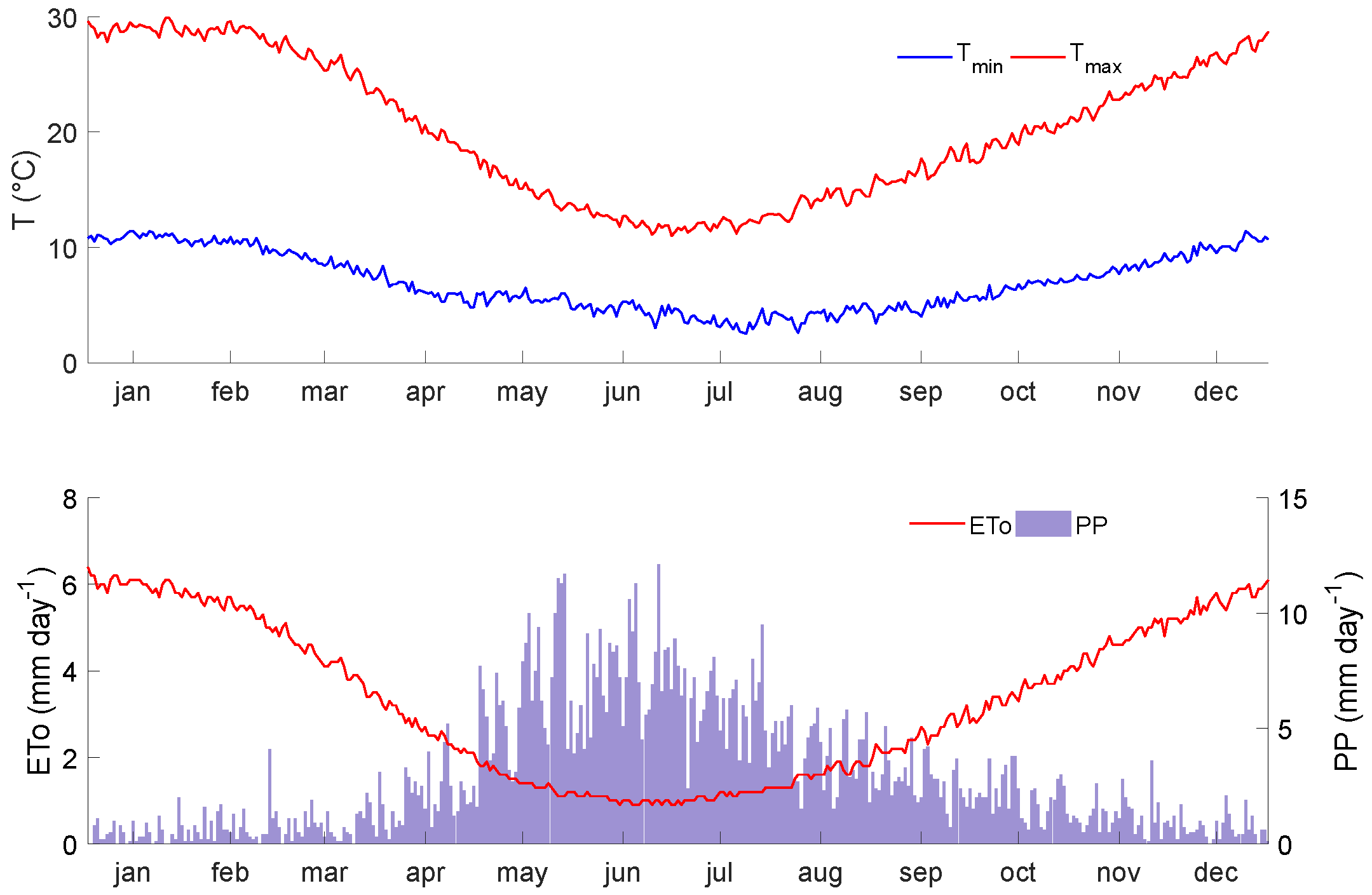
We fed our routine with: (1) characteristic sowing dates for maize (November), sugar beet (September), and wheat (August) [35]; (2) a weather database from 1965 to 2016 (Figure 3); (3) crops parameters (

Table 2. Conservative (constant) and generally applicable parameters for maize, sugar beet, and wheat [20] in the Central Valley of Chile [29].

Parameter	Crop
	Maize	Sugar Beet	Wheat
Conservative (generally applicable)
Base temperature (${}^{\circ }$C)	8.00	5.00	0.00
Cut-off temperature (${}^{\circ }$C)	30.00	30.00	26.00
Canopy cover per seedling at 90% emergence (CCo)	6.50	1.00	1.50
Canopy growth coefficient (CGC)	1.25	1.05	0.50
Maximum canopy cover (CCx)	96.00	98.00	96.00
Crop coefficient for transpiration at CC = 100%	1.05	1.10	1.10
Decline in crop coef. after reaching CCx	0.30	0.15	0.15
Canopy decline coefficient (CDC) at senescence	1.00	0.39	0.40
Water productivity, normalized to year 2000 (WP)	33.70	17.00	15.00
Leaf growth threshold (Pupper)	0.14	0.20	0.20
Leaf growth threshold (Plower)	0.72	0.60	0.65
Leaf growth stress coefficient curve shape	2.90	3.00	5.00
Stomatal conductance threshold (Pupper)	0.69	0.65	0.65
Stomata stress coefficient curve shape	6.00	3.00	2.50
Senescence stress coefficient (Pupper)	0.69	0.75	0.70
Senescence stress coefficient curve shape	2.70	3.00	2.50
Considered to be conservative but can or may be cultivar specific
Reference harvest index (HIo)	48	70	48
GDD from 90% emergence to start of anthesis	800	842	1100
Duration of anthesis, in GDD	180	0	200
Coefficient, inhibition of leaf growth on HI	7	4	10
Coefficient, inhibition of stomata on HI	3	-	7
Maximum yield (t ha−1) (more details in Kuschel-Otárola et al. [37])	15	100	7

); and (4) soil hydraulic parameters dependant on their bulk densities (

Table 3. Bulk density (${\rho }_a$), saturation (${\theta }_s$), field capacity (${\theta }_{fc}$), permanent wilt water content (${\theta }_{pwp}$), and saturated hydraulic conductivity ($K_s$) [38], as representative of the Central Valley of Chile [29,33,39].

	Sand	Silt	Clay	${\mathit{\rho }}_{\mathit{a}}$	${\mathit{\theta }}_{\mathit{s}}$	${\mathit{\theta }}_{\mathbf{f}\mathbf{c}}$	${\mathit{\theta }}_{\mathbf{pwp}}$	${\mathit{K}}_{\mathit{s}}$
Soil	(%)			(g cm−3)	(m3m−3)			(mm day−1)
ClayLoam 1	22	48	30	0.72	0.73	0.45	0.30	3415.9
ClayLoam 2	35	38	27	0.97	0.64	0.57	0.33	269.1
ClayLoam 3	39	28	33	1.39	0.47	0.34	0.26	132.4
Loam 1	34	42	24	0.71	0.73	0.44	0.28	3517.8
Loam 2	31	46	23	1.07	0.60	0.59	0.40	69.5
Loam 3	41	37	22	1.13	0.57	0.55	0.34	110.3
SiltyClayLoam 1	10	52	38	0.78	0.70	0.46	0.32	2382.0
SiltyClayLoam 2	11	52	37	0.81	0.69	0.50	0.32	1903.3
SiltyClayLoam 3	15	49	36	0.86	0.68	0.50	0.36	1534.2
SiltyLoam 1	27	50	23	0.71	0.73	0.44	0.28	3571.7
SiltyLoam 2	22	51	27	0.98	0.63	0.59	0.38	183.9
SiltyLoam 3	24	51	25	1.03	0.61	0.59	0.44	76.3

Index numbers 1, 2, and 3 correspond to soils with a low, medium, and high bulk density, respectively.

). We considered that each growing season started with 50% of the total available water (more details in Kuschel-Otárola et al. [29]).

3. Results and Discussion

3.1. Dry Yield as a Function of Water Use

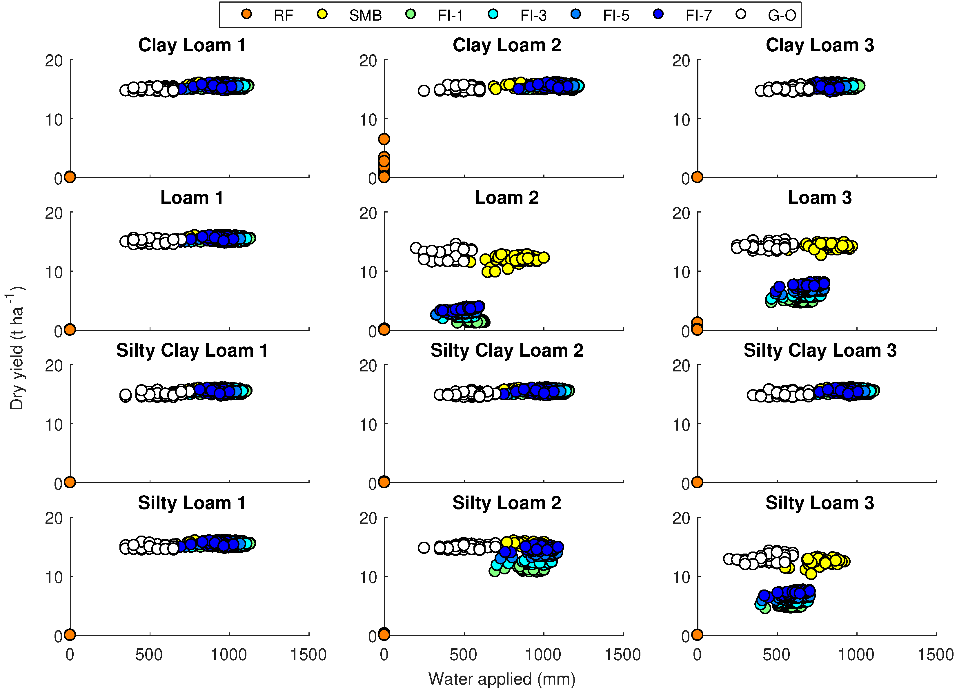
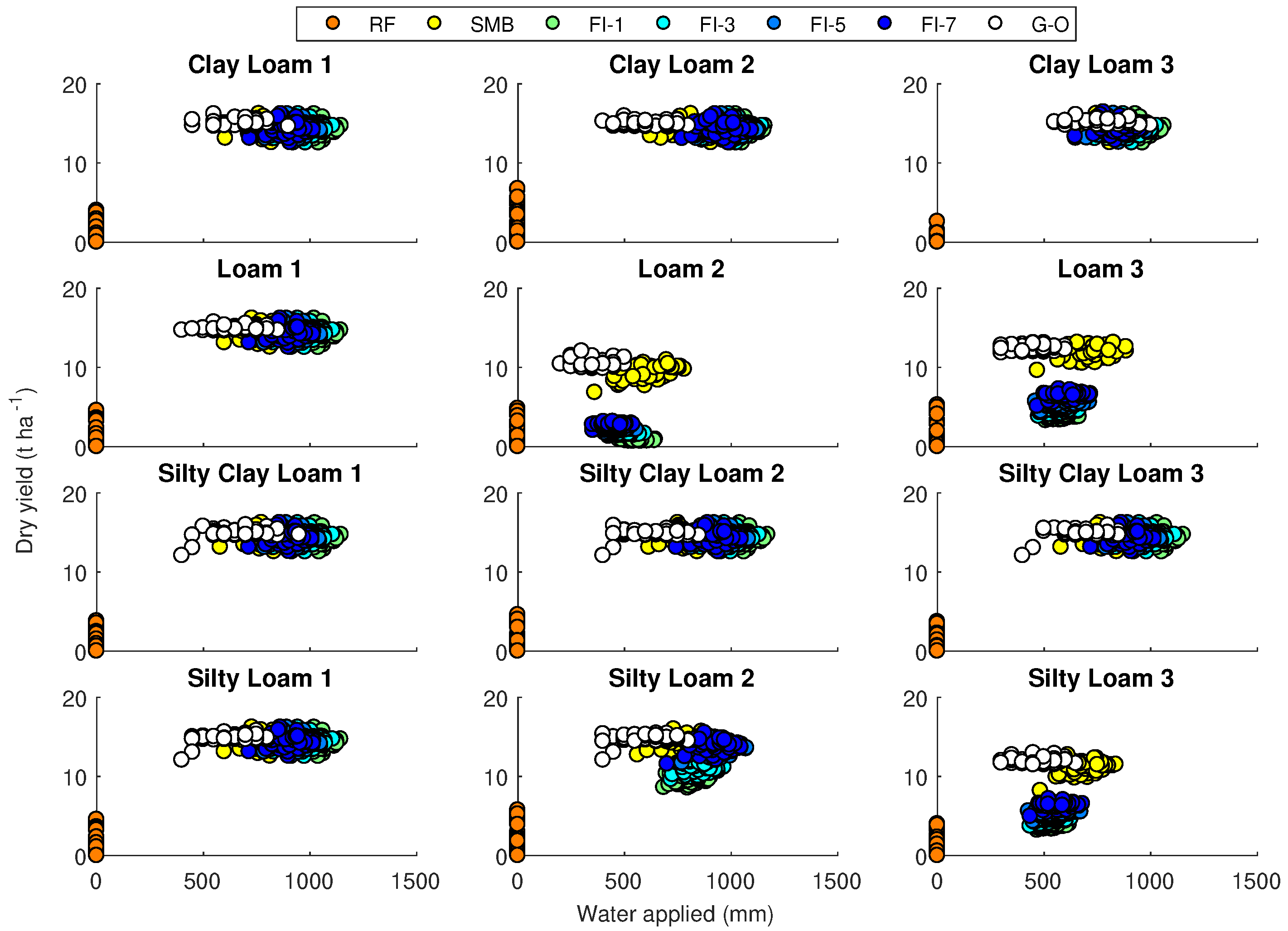
Dry yield as a function of water applied (for the whole growing season) for all irrigation strategies are presented for maize (Figure 4), sugar beet (Figure 5), and wheat (Figure 6), considering simulated values from 1965 to 2016 for soils with a low, medium, and high bulk density. These figures are presented in the form of scatter plots, in which each color represents an irrigation strategy: rainfed (RF), soil moisture-based (SMB), fixed interval (FI) every 1, 3, 5, and 7 days, and the optimal irrigation schedule (GET-OPTIS: G-O). In all cases, the best strategies are those that use less water to give higher yields. For all crops, clayey soils plateau, showing that there is an upper limit for yield regardless of the irrigation strategy. Thus, it is clear that certain strategies exist that use much less water than others. Furthermore, lighter soils (with a bulk density less than 1) display a similar behavior. Heavier loamy soils are more sensitive to irrigation strategies, as is shown by the fewer instances of overlapping grouping. These results highlight the importance of the soil texture and bulk density in crop performance.

3.1.1. Dry Yield as a Function of Water Use for Maize

Figure 4 presents dry yield as a function of water use for maize considering simulated values from 1965 to 2016 for soils with a low (1), medium (2), and high bulk density (3) (mean values in

Table A1. Dry yield (in t ha⁻¹) and water use (in mm) for maize, as a function of soil type according to irrigation strategy, as a mean value of simulated values from 1965 to 2016. Values outside and inside parentheses indicate dry yield and water use, respectively.

Soil	RF	SMB	FI-1	FI-3	FI-5	FI-7	G-O
CL1	0 ± 0.01	15.4 ± 0.27	15.45 ± 0.27	15.45 ± 0.27	15.41 ± 0.28	15.34 ± 0.28	14.9 ± 0.27
	(0 ± 0)	(867 ± 76)	(1034 ± 55)	(1006 ± 60)	(960 ± 58)	(924 ± 59)	(549 ± 81)
CL2	0.48 ± 1.16	15.38 ± 0.27	15.38 ± 0.29	15.45 ± 0.27	15.43 ± 0.27	15.39 ± 0.28	14.94 ± 0.32
	(0 ± 0)	(900 ± 74)	(1136 ± 56)	(1128 ± 60)	(1098 ± 59)	(1064 ± 59)	(503 ± 85)
CL3	0 ± 0	15.44 ± 0.27	15.45 ± 0.27	15.44 ± 0.27	15.35 ± 0.28	15.2 ± 0.3	14.95 ± 0.28
	(0 ± 0)	(836 ± 71)	(930 ± 56)	(884 ± 58)	(835 ± 56)	(798 ± 58)	(610 ± 80)
L1	0 ± 0.01	15.39 ± 0.27	15.45 ± 0.27	15.45 ± 0.27	15.42 ± 0.27	15.35 ± 0.28	14.91 ± 0.3
	(0 ± 0)	(859 ± 74)	(1038 ± 59)	(1011 ± 64)	(966 ± 62)	(930 ± 64)	(527 ± 82)
L2	0 ± 0.02	11.87 ± 0.66	1.4 ± 0.12	2.24 ± 0.08	2.87 ± 0.13	3.54 ± 0.25	12.73 ± 0.87
	(0 ± 0)	(828 ± 94)	(573 ± 31)	(511 ± 37)	(500 ± 49)	(505 ± 58)	(408 ± 82)
L3	0.04 ± 0.18	14.13 ± 0.42	4.92 ± 0.16	5.72 ± 0.15	6.66 ± 0.19	7.57 ± 0.28	14.05 ± 0.45
	(0 ± 0)	(832 ± 79)	(648 ± 49)	(684 ± 58)	(697 ± 60)	(707 ± 64)	(452 ± 87)
SCL1	0 ± 0	15.4 ± 0.27	15.45 ± 0.27	15.45 ± 0.27	15.41 ± 0.28	15.33 ± 0.28	14.9 ± 0.34
	(0 ± 0)	(862 ± 79)	(1023 ± 54)	(994 ± 60)	(948 ± 59)	(911 ± 60)	(561 ± 91)
SCL2	0 ± 0.02	15.39 ± 0.27	15.45 ± 0.27	15.45 ± 0.27	15.42 ± 0.27	15.36 ± 0.28	14.9 ± 0.29
	(0 ± 0)	(882 ± 69)	(1075 ± 55)	(1052 ± 60)	(1012 ± 59)	(975 ± 59)	(540 ± 80)
SCL3	0 ± 0	15.4 ± 0.27	15.45 ± 0.27	15.45 ± 0.27	15.4 ± 0.28	15.32 ± 0.28	14.93 ± 0.32
	(0 ± 0)	(876 ± 76)	(1025 ± 54)	(998 ± 59)	(954 ± 59)	(917 ± 60)	(565 ± 87)
SL1	0 ± 0.01	15.39 ± 0.27	15.45 ± 0.27	15.45 ± 0.27	15.42 ± 0.27	15.35 ± 0.28	14.89 ± 0.33
	(0 ± 0)	(859 ± 74)	(1038 ± 59)	(1011 ± 64)	(966 ± 62)	(930 ± 64)	(535 ± 83)
SL2	0.01 ± 0.04	15.34 ± 0.28	11.21 ± 0.27	12.36 ± 0.26	13.79 ± 0.37	14.62 ± 0.29	14.84 ± 0.33
	(0 ± 0)	(890 ± 78)	(920 ± 57)	(958 ± 63)	(987 ± 65)	(990 ± 68)	(515 ± 97)
SL3	0 ± 0	12.31 ± 0.52	4.91 ± 0.16	5.61 ± 0.15	6.39 ± 0.19	7.16 ± 0.28	12.98 ± 0.58
	(0 ± 0)	(778 ± 76)	(582 ± 43)	(605 ± 56)	(611 ± 58)	(616 ± 63)	(454 ± 89)

Soil types: CL: Clay Loam; L: Loam; SCL: Silty Clay Loam; SL: Silty Loam for low (1), medium (2), and high (3) bulk density. Irrigation strategies: RF: Rainfed; SMB: Soil moisture-based; FI: Fixed Interval every 1, 3, 5, and 7 days; G-O: GET-OPTIS.

). The results showed that G-O consistently provides the best combination of dry yield and water use, followed by SMB. G-O could save from 105 (for clay loam 3 considering FI-1 for the year 1979) to 827 mm (for clay loam 2 considering FI-3 for the year 2013) of water. For the year 1979 under clay loam 3, G-O and FI-1 achieved dry yield values of 15.21 and 14.92 t ha⁻¹, respectively. For the year 2013 under clay loam 2, G-O and FI-3 achieved dry yield values of 14.81 and 15.35 t ha⁻¹, respectively. According to the study area, irrigation depth for maize ranges from 400 to 800 [40,41] to produce a mean value of 15 t ha⁻¹ [37,40,42]. There are low values of dry yield for loam 2, loam 3, and silty loam 3 considering fixed irrigation strategies. These soils have a very narrow range between saturation and field capacity (see Table 3), where crop production is mainly affected by the stress produced by conditions of lack of aeration in the root zone [22,43], when moisture reaches a value of at least 5% below saturation.

3.1.2. Dry Yield as a Function of Water Use for Sugar Beet

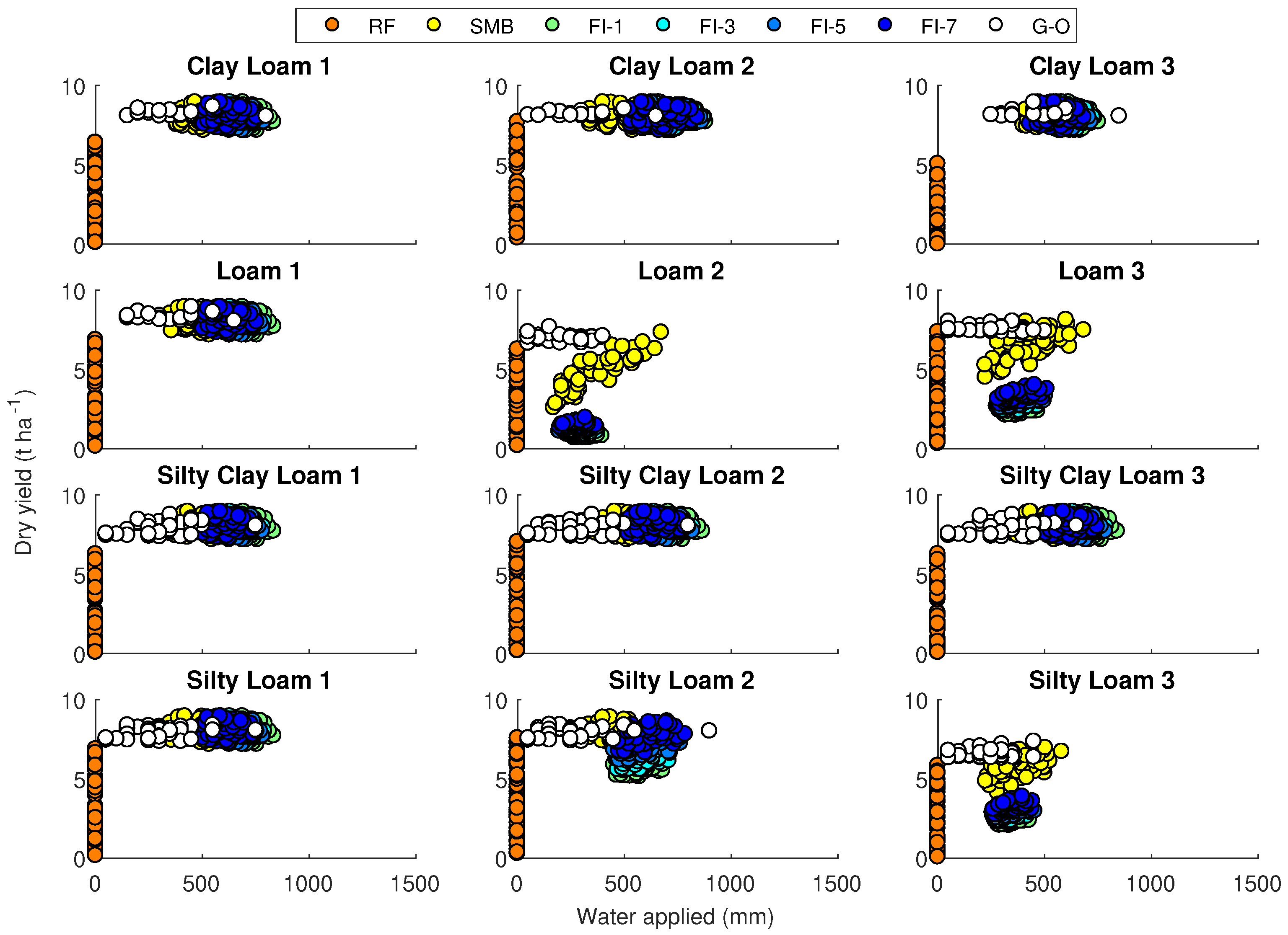
Figure 5 presents dry yield as a function of water use for sugar beet considering simulated values from 1965 to 2016 for soils with a low (1), medium (2), and high bulk density (3) (mean values in

Table A2. Dry yield (in t ha⁻¹) and water use (in mm) for sugar beet, as a function of soil type according to irrigation strategy, as a mean value of simulated values from 1965 to 2016. Values outside and inside parentheses indicate dry yield and water use, respectively.

Soil	RF	SMB	FI-1	FI-3	FI-5	FI-7	G-O
CL1	0.9 ± 1.19	14.31 ± 0.76	14.28 ± 0.76	14.28 ± 0.76	14.29 ± 0.76	14.31 ± 0.76	14.41 ± 2.93
	(0 ± 0)	(823 ± 77)	(1038 ± 52)	(981 ± 58)	(936 ± 61)	(906 ± 64)	(654 ± 161)
CL2	1.58 ± 1.76	14.31 ± 0.76	14.28 ± 0.76	14.28 ± 0.76	14.28 ± 0.76	14.28 ± 0.76	14.36 ± 2.91
	(0 ± 0)	(849 ± 89)	(1043 ± 62)	(1016 ± 68)	(986 ± 72)	(963 ± 76)	(585 ± 152)
CL3	0.25 ± 0.5	14.32 ± 0.76	14.28 ± 0.76	14.29 ± 0.76	14.35 ± 0.76	14.53 ± 0.76	14.55 ± 2.95
	(0 ± 0)	(822 ± 60)	(954 ± 55)	(912 ± 59)	(863 ± 58)	(835 ± 61)	(737 ± 184)
L1	1.16 ± 1.41	14.31 ± 0.76	14.28 ± 0.76	14.28 ± 0.76	14.28 ± 0.76	14.3 ± 0.76	14.36 ± 2.91
	(0 ± 0)	(809 ± 78)	(1038 ± 52)	(981 ± 59)	(936 ± 62)	(906 ± 64)	(632 ± 162)
L2	1.17 ± 1.49	9.39 ± 0.86	0.83 ± 0.1	1.59 ± 0.11	2.18 ± 0.14	2.74 ± 0.2	10.49 ± 0.49
	(0 ± 0)	(619 ± 91)	(565 ± 38)	(497 ± 44)	(463 ± 50)	(447 ± 51)	(354 ± 70)
L3	1.52 ± 1.71	11.89 ± 0.8	3.84 ± 0.25	4.58 ± 0.28	5.42 ± 0.33	6.36 ± 0.42	12.41 ± 0.35
	(0 ± 0)	(726 ± 88)	(585 ± 44)	(571 ± 53)	(589 ± 60)	(609 ± 61)	(441 ± 83)
SCL1	0.76 ± 1.04	14.31 ± 0.76	14.28 ± 0.76	14.28 ± 0.76	14.29 ± 0.76	14.31 ± 0.76	14.86 ± 0.58
	(0 ± 0)	(827 ± 74)	(1039 ± 51)	(979 ± 57)	(933 ± 60)	(902 ± 63)	(678 ± 110)
SCL2	1.12 ± 1.42	14.31 ± 0.76	14.28 ± 0.76	14.28 ± 0.76	14.28 ± 0.76	14.29 ± 0.76	14.83 ± 0.66
	(0 ± 0)	(826 ± 89)	(1060 ± 54)	(1001 ± 61)	(960 ± 65)	(931 ± 67)	(644 ± 108)
SCL3	0.7 ± 1	14.31 ± 0.76	14.28 ± 0.76	14.28 ± 0.76	14.29 ± 0.76	14.31 ± 0.76	14.88 ± 0.55
	(0 ± 0)	(831 ± 79)	(1046 ± 51)	(983 ± 57)	(938 ± 60)	(908 ± 63)	(689 ± 100)
SL1	1.16 ± 1.41	14.31 ± 0.76	14.28 ± 0.76	14.28 ± 0.76	14.28 ± 0.76	14.3 ± 0.76	14.83 ± 0.54
	(0 ± 0)	(809 ± 78)	(1038 ± 52)	(981 ± 59)	(936 ± 62)	(906 ± 64)	(656 ± 107)
SL2	1.42 ± 1.74	14.02 ± 0.77	9.68 ± 0.55	10.96 ± 0.61	13.47 ± 0.76	13.68 ± 0.79	14.72 ± 0.54
	(0 ± 0)	(819 ± 92)	(804 ± 53)	(849 ± 60)	(934 ± 70)	(919 ± 75)	(614 ± 106)
SL3	0.72 ± 1.09	11.02 ± 0.82	3.8 ± 0.24	4.51 ± 0.28	5.32 ± 0.33	6.23 ± 0.42	11.96 ± 0.36
	(0 ± 0)	(690 ± 75)	(536 ± 39)	(527 ± 47)	(546 ± 54)	(569 ± 55)	(468 ± 85)

Soil types: CL: Clay Loam; L: Loam; SCL: Silty Clay Loam; SL: Silty Loam for low (1), medium (2), and high (3) bulk density. Irrigation strategies: RF: Rainfed; SMB: Soil moisture-based; FI: Fixed Interval every 1, 3, 5, and 7 days; G-O: GET-OPTIS.

). Similar to maize, G-O was the strategy that provided the best combination of dry yield and water use, followed by SMB. G-O could save from 48 (for silty loam 3 considering SMB for the year 1979) to 684 mm (for clay loam 2 considering FI-1 for the year 2008) of water. For the year 1979 under silty loam 3, G-O and SMB achieved dry yield values of 12.07 and 8.19 t ha⁻¹, respectively. For the year 2008 under clay loam 2, G-O and FI-1 achieved dry yield values of 15.25 and 14.17 t ha⁻¹, respectively. According to the study area, the irrigation depth for sugar beet has a mean value of 800 mm [40]. The results showed that sugar beet has a potential dry yield of 16 t ha⁻¹, but considering 14–20% sucrose on a fresh mass basis [28], the fresh yield can achieve values from 80 to 114 t ha⁻¹ [29]. Farmers of the study area have a mean fresh yield value of 105 t ha ⁻¹ [37,40]. Similar to maize, there are low values of dry yield for loam 2, loam 3, and silty loam 3 considering fixed irrigation strategies.

3.1.3. Dry Yield as a Function of Water Use for Wheat

Figure 6 presents dry yield as a function of water use for wheat, considering simulated values from 1965 to 2016 for soils with a low (1), medium (2), and high bulk density (3) (mean values in

Table A3. Dry yield (in t ha⁻¹) and water use (in mm) for wheat, as a function of soil type according to irrigation strategy, as a mean value of simulated values from 1965 to 2016. Values outside and inside parentheses indicate dry yield and water use, respectively.

Soil	RF	SMB	FI-1	FI-3	FI-5	FI-7	G-O
CL1	2.79 ± 1.95	8.01 ± 0.47	8.01 ± 0.47	8.01 ± 0.47	8.01 ± 0.47	8.01 ± 0.47	3.8 ± 4.15
	(0 ± 0)	(525 ± 90)	(715 ± 55)	(664 ± 61)	(637 ± 68)	(617 ± 67)	(170 ± 208)
CL2	4.01 ± 2.14	8.01 ± 0.47	8 ± 0.47	8 ± 0.47	8 ± 0.47	8 ± 0.47	3.78 ± 4.12
	(0 ± 0)	(545 ± 104)	(727 ± 75)	(706 ± 80)	(688 ± 85)	(673 ± 85)	(135 ± 174)
CL3	1.3 ± 1.43	8.01 ± 0.47	8.01 ± 0.47	8.01 ± 0.47	8.01 ± 0.47	8.01 ± 0.47	3.96 ± 4.16
	(0 ± 0)	(519 ± 71)	(633 ± 55)	(604 ± 59)	(582 ± 63)	(564 ± 63)	(229 ± 257)
L1	3.19 ± 2.02	8.01 ± 0.47	8.01 ± 0.47	8.01 ± 0.47	8.01 ± 0.47	8.01 ± 0.47	3.99 ± 4.18
	(0 ± 0)	(513 ± 84)	(715 ± 55)	(663 ± 60)	(636 ± 67)	(616 ± 67)	(167 ± 196)
L2	3.05 ± 1.7	4.89 ± 1.14	0.81 ± 0.07	1.07 ± 0.09	1.28 ± 0.11	1.5 ± 0.16	4.69 ± 3.31
	(0 ± 0)	(372 ± 133)	(319 ± 32)	(286 ± 35)	(270 ± 41)	(263 ± 40)	(156 ± 137)
L3	3.67 ± 1.95	6.49 ± 0.9	2.45 ± 0.19	2.74 ± 0.21	3.04 ± 0.25	3.33 ± 0.3	5.96 ± 3.12
	(0 ± 0)	(436 ± 114)	(376 ± 41)	(361 ± 48)	(377 ± 57)	(377 ± 60)	(209 ± 152)
SCL1	2.6 ± 1.88	8.01 ± 0.47	8.01 ± 0.47	8.01 ± 0.47	8.01 ± 0.47	8.01 ± 0.47	6.29 ± 3.31
	(0 ± 0)	(515 ± 84)	(716 ± 54)	(662 ± 58)	(634 ± 66)	(613 ± 65)	(264 ± 196)
SCL2	3.26 ± 2.08	8.01 ± 0.47	8.01 ± 0.47	8.01 ± 0.47	8.01 ± 0.47	8.01 ± 0.47	6.19 ± 2.95
	(0 ± 0)	(536 ± 101)	(735 ± 60)	(683 ± 66)	(657 ± 73)	(637 ± 72)	(238 ± 168)
SCL3	2.57 ± 1.89	8.01 ± 0.47	8.01 ± 0.47	8.01 ± 0.47	8.01 ± 0.47	8.01 ± 0.47	6.3 ± 3.31
	(0 ± 0)	(522 ± 83)	(722 ± 54)	(665 ± 58)	(637 ± 66)	(615 ± 65)	(252 ± 177)
SL1	3.19 ± 2.02	8.01 ± 0.47	8.01 ± 0.47	8.01 ± 0.47	8.01 ± 0.47	8.01 ± 0.47	6.26 ± 3.29
	(0 ± 0)	(513 ± 84)	(715 ± 55)	(663 ± 60)	(636 ± 67)	(616 ± 67)	(242 ± 181)
SL2	3.88 ± 2.19	7.94 ± 0.48	5.73 ± 0.38	6.24 ± 0.44	7.07 ± 0.56	7.56 ± 0.55	6.27 ± 3.29
	(0 ± 0)	(517 ± 103)	(557 ± 59)	(568 ± 68)	(596 ± 81)	(606 ± 84)	(222 ± 180)
SL3	2.55 ± 1.72	5.67 ± 0.68	2.42 ± 0.19	2.68 ± 0.21	2.97 ± 0.23	3.23 ± 0.28	5.45 ± 2.53
	(0 ± 0)	(385 ± 91)	(341 ± 35)	(328 ± 39)	(342 ± 47)	(341 ± 48)	(197 ± 127)

Soil types: CL: Clay Loam; L: Loam; SCL: Silty Clay Loam; SL: Silty Loam for low (1), medium (2), and high (3) bulk density. Irrigation strategies: RF: Rainfed; SMB: Soil moisture-based; FI: Fixed Interval every 1, 3, 5, and 7 days; G-O: GET-OPTIS.

). The results showed that RF was the strategy with the lowest water use (no irrigation), achieving maximum dry yield values from 5.1 (for clay loam 3) to 7.7 t ha⁻¹ (for clay loam 2). The sowing date for wheat was assumed to be 1 August, when water demand is satisfied by water from rainfall. However, if wheat is irrigated (and considering both mentioned soils), dry yield could increase from 5.06 to 8.95 t ha⁻¹ for clay loam 3 (applying 250 mm of water, considering G-O) and from 7.71 to 8.95 t ha⁻¹ for clay loam 2 (applying only 50 mm of water, considering G-O). For clay loam 3, the maximum dry yield value for SMB, FI-1, FI-3, FI-5, FI-7, and G-O was 8.9 t ha⁻¹, but G-O applied the lowest amount of water (250 mm), followed by SMB (400 mm). For clay loam 2, the maximum dry yield for SMB, FI-1, FI-3, FI-5 and FI-7 was 8.9 t ha⁻¹. However, G-O achieved a maximum dry yield of 8.5 t ha⁻¹ and applied the lowest amount of water (50 mm, compared to 340 mm considering SMB). Similar to maize and sugar beet, low dry yield values were attained for loam 2, loam 3, and silty loam 3 considering fixed irrigation strategies.

In terms of the impacts of water use, the best strategy is GET-OPTIS. On the other hand, achieving high irrigation efficiency leads to energy savings. There is a bias towards pressurized systems, but this increases greenhouse gas emissions. Therefore, highly automated furrow irrigation could be an option [44,45].

However, implementing irrigation strategies such as GET-OPTIS and soil moisture-based irrigation requires an important investment in monitoring crop conditions, as well as workers to operate the system in the field. There is also the need for improved weather forecasting and better designs.

3.2. Economic Analysis

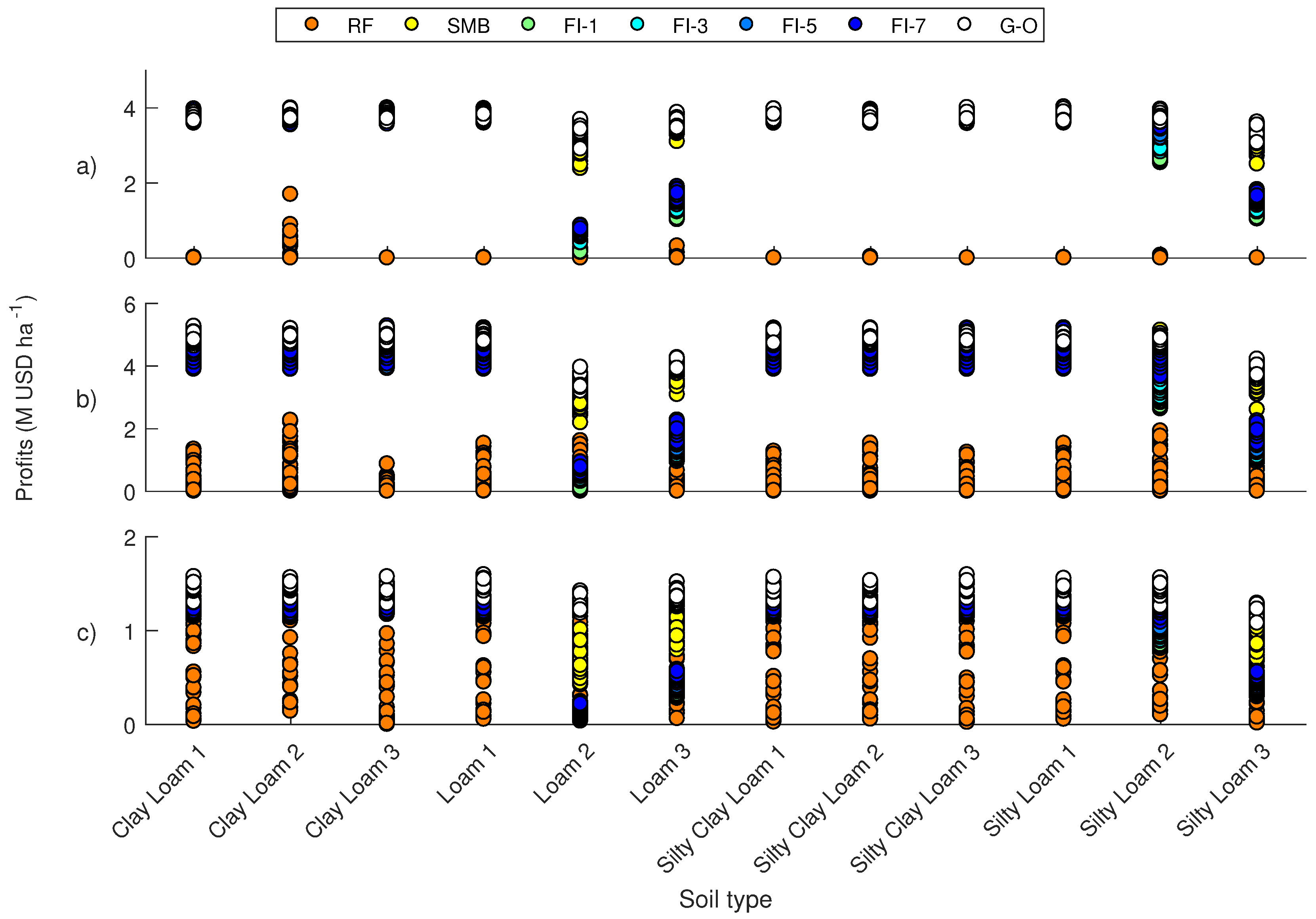
The differences between income and cost associated with irrigation for each irrigation strategy are presented in Figure 7, considering simulated values from 1965 to 2016 for soils with a low, medium, and high bulk density. Similar to Figure 4, Figure 5 and Figure 6, the results are presented in the form of scatter plots, in which each color represents an irrigation strategy. The results showed that G-O was the strategy with the largest profits for most of the combinations of crop and soil types.

However, it is worth noting that the implementation and operation of sophisticated irrigation schedules such as G-O requires better design criteria that account for soil variability and not only for topography [46]. A second issue is the need for better automatization and control systems within farms [47,48]. A third important issue is the fact that in Chile, the price of water is negligible, so most economic analyses advise against incorporating control systems [49,50].

3.3. Water Use Efficiency

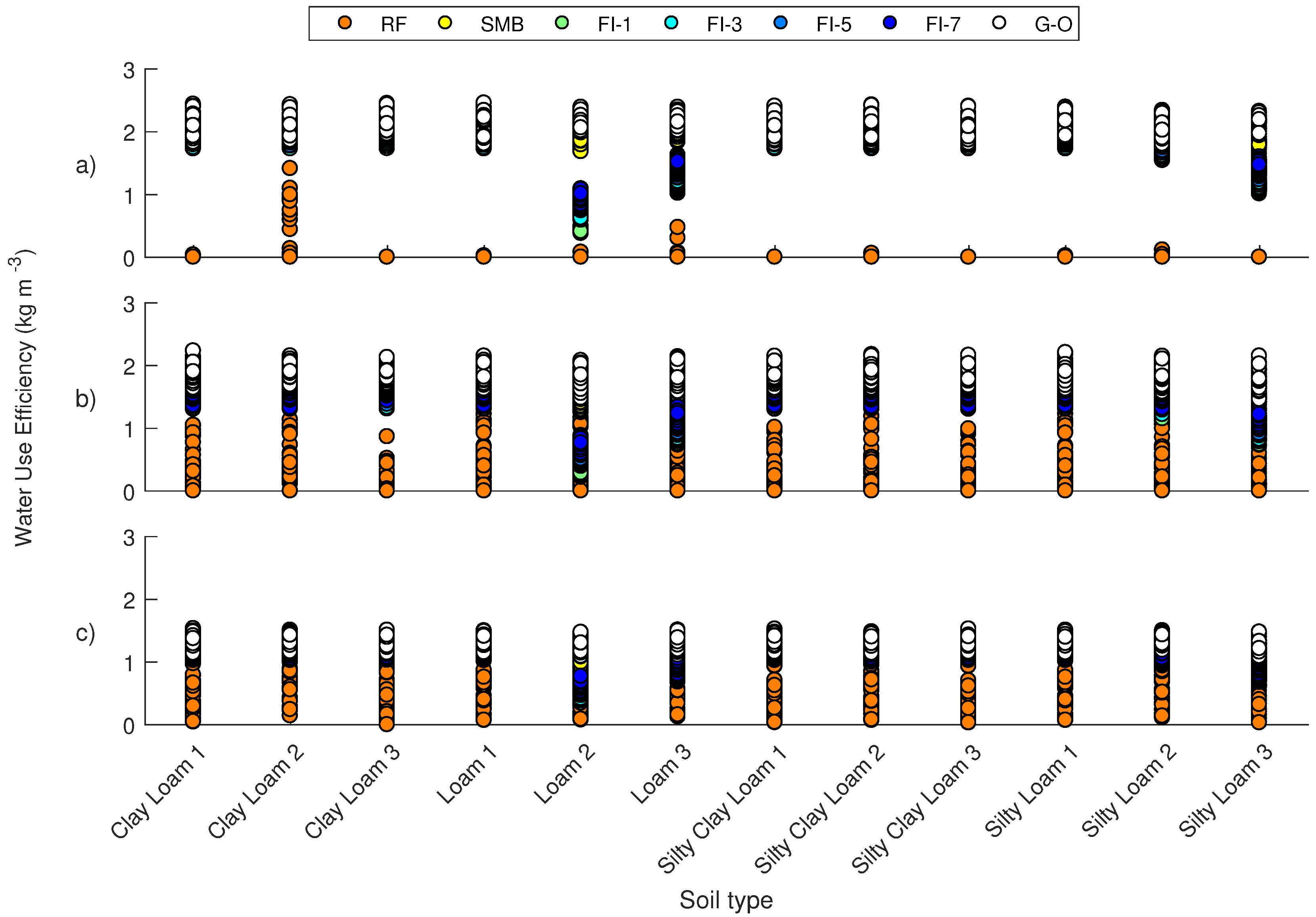
Water-use efficiency (WUE) as a function of crops for all irrigation strategies are presented in Figure 8, considering simulated values from 1965 to 2016 for soils with a low, medium, and high bulk density. Similar to Figure 4, Figure 5, Figure 6 and Figure 7, the results are presented in the form of scatter plots, in which each color represents an irrigation strategy. The results showed that G-O was the strategy with the highest WUE (from 1.47 kg m⁻³ for wheat in loam 2 soil to 2.46 kg m⁻³ for maize in the same soil).

For maize, the best strategy was G-O (from 1.80 to 2.46 kg m⁻³), followed by SMB (from 1.64 to 2.19 kg m⁻³), and FI-7 (from 0.84 to 2.23 kg m⁻³). On the other hand, the strategies with the lowest performance were RF, FI-1, and FI-3. As Chile is characterized by a mediterranean climate, WUE for maize ranges from 1.50 to 2.16 kg m⁻³ [51]. Regarding sugar beet and similar to maize, G-O achieved the best performance for WUE (from 1.46 to 2.23 kg m⁻³), followed by SMB (from 1.25 to 1.94 kg m⁻³), and FI-7 (from 0.60 to 1.91 kg m⁻³). On the other hand, the strategies with the lowest performance were RF, FI-1, and FI-3. According to Katerji et al. [51], WUE for sugar beet ranges from 6.60 to 7.00 kg m⁻³ in Spain, but considering that farmers in Chile achieve a mean fresh yield value of 105 t ha⁻³ [40], this WUE on a fresh mass basis reaches values from 10 to 14 kg m⁻³. For wheat and similar to maize and sugar beet, G-O achieved the highest performance for WUE (from 1.07 to 1.53 kg m⁻³), followed by SMB (from 0.82 to 1.51 kg m⁻³), and FI-7 (from 0.52 to 1.44 kg m⁻³). Katerji et al. [51] reported WUE values from 1.0 to 1.5 kg m⁻³ in mediterranean zones. On the other hand, the strategies with the lowest performance were FI-1 and FI-3. Unlike maize and sugar beet, RF achieved high values for WUE (with values over 1.20 kg m⁻³). This is due to the considered sowing date (early August) when wheat can be watered by rainfall. The harvest date for wheat is between December and January, demanding less water compared to maize and sugar beet. Thus, soil type has an important influence on the yield and performance of different irrigation strategies.

Regarding soil water holding capacity (SWHC), SMB demonstrated a better performance when SWHC was greater than 0.1 m³ m⁻³ (Loam 1–2, Silty Loam 1, Silty Clay Loam 2) for maize. For sugar beet, the best strategies were G-O, SMB, and FI-7, while the worst were RF, FI-1, and FI-3. Similar to sugar beet, the best strategies for wheat were G-O, SMB, and FI-7. However, SWHC values over 0.18 m³ m⁻³ (Silty Clay Loam 2, Loam 2–3, Silty Loam 2 and Clay Loam 2) demonstrate the superior performance of RF.

4. Conclusions

Irrigation is one of the main factors for crop development, therefore we developed a methodology to estimate crop yield and water-use efficiency for different irrigation strategies. We calculated crop yield and its respective water use to estimate water-use efficiency considering local crops, soils, weather conditions, sowing dates, and field management methods. This methodology was assessed using 52 years of weather data (from 1965 to 2016) and seven irrigation management methods (rainfed, soil moisture-based, a fixed interval every 1, 3, 5, and 7 days, and a problem-specific algorithm for optimal irrigation scheduling with limited water supply (GET-OPTIS)). The results showed that GET-OPTIS was the methodology with the best performance (with highest crop yield values, lowest water use, and highest WUE and profits according to the economic analysis), followed by soil moisture-based management. To implement both strategies, an important investment in monitoring crop conditions is required, as well as the design of irrigation systems that take into account irrigation criteria and management. Furthermore, the need for improved weather forecasts and better designs is also crucial. Future studies should focus on the validation of AquaCrop-OS under local conditions, which include GET-OPTIS, to produce “more crop per drop”. This work can serve as a methodological guide for simulating water-use efficiency of crops and can be used alongside evidence from the field.

References

- Wichelns, D.; Oster, J.D. Sustainable irrigation is necessary and achievable, but direct costs and environmental impacts can be substantial. Agric. Water Manag. 2006, 86, 114–127. [Google Scholar] [CrossRef]
- FAO. AQUASTAT website. In FAO’s Information System on Water and Agriculture; Food and Agriculture Organization of the United Nations: Rome, Italy, 2016. [Google Scholar]
- Hubick, K.T.; Farquhar, G.D.; Shorter, R. Correlation between water use efficiency and carbon isotope discrimination in diverse peanut (Arachis) germplasm. Aust. J. Plant Physiol. 1986, 13, 803–816. [Google Scholar] [CrossRef]
- Saccon, P. Water for agriculture, irrigation management. Appl. Soil Ecol. 2017. [Google Scholar] [CrossRef]
- Malik, A.; Shakir, A.; Ajmal, M.; Khan, M.; Khan, T. Assessment of AquaCrop model in simulating sugar beet canopy cover, biomass and root yield under different irrigation and field management practices in semi-arid regions of Pakistan. Water Resour. Manag. 2017, 31, 4275–4292. [Google Scholar] [CrossRef]
- Steduto, P.; Hsiao, T.; Raes, D.; Fereres, E. AquaCrop—The FAO crop model to simulate yield response to water: I. Concepts and underlying principles. Agron. J. 2009, 101, 426–437. [Google Scholar] [CrossRef]
- Paredes, P.; de Melo-Abreu, J.; Alves, I.; Pereira, L.S. Assessing the performance of the FAO AquaCrop model to estimate maize yields and water use under full and deficit irrigation with focus on model parameterization. Agric. Water Manag. 2014, 144, 81–97. [Google Scholar] [CrossRef]
- Nyakudya, I.W.; Stroosnijder, L. Effect of rooting depth, plant density and planting date on maize (Zea mays L.) yield and water use efficiency in semi-arid Zimbabwe: Modeling with AquaCrop. Agric. Water Manag. 2014, 146, 280–296. [Google Scholar] [CrossRef]
- Heng, L.K.; Hsiao, T.; Evett, S.; Howell, T.; Steduto, P. Validating the FAO AquaCrop model for irrigated and water deficient field maize. Agron. J. 2009, 101, 488–498. [Google Scholar] [CrossRef]
- Toumi, J.; Er-Raki, S.; Ezzahar, J.; Khabba, S.; Jarlan, L.; Chehbouni, A. Performance assessment of AquaCrop model for estimating evapotranspiration, soil water content and grain yield of winter wheat in Tensift Al Haouz (Morocco): Application to irrigation management. Agric. Water Manag. 2016, 163, 219–235. [Google Scholar] [CrossRef]
- Mkhabela, M.S.; Paul, R.B. Performance of the FAO AquaCrop model for wheat grain yield and soil moisture simulation in Western Canada. Agric. Water Manag. 2012, 110, 16–24. [Google Scholar] [CrossRef]
- Andarzian, B.; Bannayan, M.; Steduto, P.; Mazraeh, H.; Barati, M.E.; Barati, M.A.; Rahnama, A. Validation and testing of the AquaCrop model under full and deficit irrigated wheat production in Iran. Agric. Water Manag. 2011, 100, 1–8. [Google Scholar] [CrossRef]
- Alishiri, R.; Paknejad, F.; Aghayari, F. Simulation of sugarbeet growth under different water regimes and nitrogen levels by AquaCrop. Int. J. Biosci. 2014, 4, 1–9. [Google Scholar]
- Stricevic, R.; Cosic, M.; Djurovic, N.; Pejic, B.; Maksimovic, L. Assessment of the FAO AquaCrop model in the simulation of rainfed and supplementally irrigated maize, sugar beet and sunflower. Agric. Water Manag. 2011, 98, 1615–1621. [Google Scholar] [CrossRef]
- Montoya, F.; Camargo, D.; Ortega, J.; Córcoles, J.; Domínguez, A. Evaluation of AquaCrop model for a potato crop under different irrigation conditions. Agric. Water Manag. 2016, 164, 267–280. [Google Scholar] [CrossRef]
- Garcia-Vila, M.; Fereres, E. Combining the simulation crop model AquaCrop with an economic model for the optimization of irrigation management at farm level. Eur. J. Agron. 2012, 36, 21–31. [Google Scholar] [CrossRef]
- Araya, A.; Habtu, S.; Hagdu, K.M.; Kebede, A.; Dejene, T. Test of AquaCrop model in simulating biomass and yield of water deficient and irrigated barley (Hordeum vulgare). Agric. Water Manag. 2010, 97, 1838–1846. [Google Scholar] [CrossRef]
- Geerts, S.; Raes, D.; Garcia, M.; Miranda, R.; Cusicanqui, J.A.; Taboada, C.; Mendoza, J.; Huanca, R.; Mamani, A.; Condori, O.; et al. Simulating yield response of quinoa to water availability with AquaCrop. Agron. J. 2009, 101, 499–508. [Google Scholar] [CrossRef]
- Maniruzzaman, M.; Talukder, M.S.U.; Khan, M.H.; Biswas, J.C.; Nemes, A. Validation of the AquaCrop model for irrigated rice production under varied water regimes in Bangladesh. Agric. Water Manag. 2015, 159, 331–340. [Google Scholar] [CrossRef]
- Foster, T.; Brozovic, N.; Butler, A.; Neale, C.; Raes, D.; Steduto, P.; Fereres, E.; Hsiao, T. AquaCrop-OS: An open source version of FAO’s crop water productivity model. Agric. Water Manag. 2017, 181, 18–22. [Google Scholar] [CrossRef]
- Viets, F., Jr. Increasing water use efficiency by soil management. In Plant Environment and Efficient Water Use; Pierre, W., Kirkham, D., Pesek, J., Shaw, R., Eds.; American Society of Agronomy: Madison, WI, USA, 1966; pp. 259–274. 295p. [Google Scholar]
- Greaves, G.; Wang, Y.M. Assessment of FAO AquaCrop model for simulating maize growth and productivity under deficit irrigation in a tropical environment. Water 2016, 8, 557. [Google Scholar] [CrossRef]
- Irmak, S. Interannual variation in Long-Term Center Pivot–irrigated maize evapotranspiration and various water productivity response indices. II: Irrigation water use efficiency, crop WUE, evapotranspiration WUE, irrigation-evapotranspiration use efficiency, and pr. J. Irrig. Drain. Eng. 2014, 141, 04014069. [Google Scholar] [CrossRef]
- Haghverdi, A.; Yonts, C.; Reichert, D.; Irmak, S. Impact of irrigation, surface residue cover and plant population on sugarbeet growth and yield, irrigation water use efficiency and soil water dynamics. Agric. Water Manag. 2017, 180, 1–12. [Google Scholar] [CrossRef]
- Hassanli, A.; Ahmadirad, S.; Beecham, S. Evaluation of the influence of irrigation methods and water quality on sugar beet yield and water use efficiency. Agric. Water Manag. 2010, 97, 357–362. [Google Scholar] [CrossRef]
- Xiangxiang, W.; Quanjiu, W.; Jun, F.; Qiuping, F. Evaluation of the AquaCrop model for simulating the impact of water deficits and different irrigation regimes on the biomass and yield of winter wheat grown on China’s Loess Plateau. Agric. Water Manag. 2013, 129, 95–104. [Google Scholar] [CrossRef]
- Schütze, N.; de Paly, M.; Shamir, U. Novel simulation-based algorithms for optimal open-loop and closed-loop scheduling of deficit irrigation systems. J. Hydroinform. 2012, 14, 136–151. [Google Scholar] [CrossRef]
- Steduto, P.; Hsiao, T.C.; Fereres, E.; Raes, D. Crop yield response to water. In FAO Irrigation and Drainage Paper 66; Food and Agriculture Organization of the United Nations: Rome, Italy, 2012; p. 503. [Google Scholar]
- Kuschel-Otárola, M.; Schütze, N.; Holzapfel, E.; Godoy-Faúndez, A.; Mialyk, O.; Rivera, D. Estimation of yield response factor for each growth stage under local conditions using AquaCrop-OS. Water 2020, 12, 1080. [Google Scholar] [CrossRef]
- DGA. Diagnóstico y Clasificación de los Cursos y Cuerpos de Agua Según Objetivo y Calidad: Cuenca del río Itata; Dirección General de Aguas: Santiago, Chile, 2004; pp. 1–127. [Google Scholar]
- ODEPA. Región del Biobío: Información Regional 2018; Oficina de Estudios y Políticas Agrarias: Santiago, Chile, 2018; pp. 1–16.
- Rivera, D.; Granda, S.; Arumí, J.L.; Sandoval, M.; Billib, M. A methodology to identify representative configurations of sensors for monitoring soil moisture. Environ. Monit. Assess. 2011, 184, 6563–6574. [Google Scholar] [CrossRef] [PubMed]
- Granda, S.; Rivera, D.; Arumí, J.L.; Sandoval, M. Monitoreo continuo de humedad con fines hidrológicos. Tecnol. Cienc. Agua 2013, 4, 189–197. [Google Scholar]
- Rivera, D.; Sandoval, M.; Godoy, A. Exploring soil databases: A self-organizing map approach. Soil Use Manag. 2015, 31, 121–131. [Google Scholar] [CrossRef]
- Faiguenbaum, H. Labranza, Siembra y Producción de Los Principales Cultivos de Chile; Vivaldi y Asociados: Santiago, Chile, 2003; p. 760. [Google Scholar]
- Walter, I.A.; Allen, R.G.; Elliott, R.; Itenfisu, D.; Brown, P.; Jensen, M.E.; Mecham, B.; Howell, T.A.; Snyder, R.; Eching, S.; et al. Task Committee on Standardization of Reference Evapotranspiration; ASCE: Reston, VA, USA, 2005. [Google Scholar]
- Kuschel-Otárola, M.; Rivera, D.; Holzapfel, E.; Palma, C.D.; Godoy-Faúndez, A. Multiperiod optimisation of irrigated crops under different conditions of water availability. Water 2018, 10, 1434. [Google Scholar] [CrossRef]
- Van Genuchten, M.T.; Leij, F.J.; Yates, S.R. The RETC Code for Quantifying the Hydraulic Functions of Unsaturated Soils. In EPA/600/2-91/065; U.S. Environmental Protection Agency: Washington, DC, USA, 1991; p. 85. [Google Scholar]
- Kuschel-Otárola, M. Estimación de Flujos de Agua en un Andisol Usando Datos de Humedad. Bachelor’s Thesis, Universidad de Concepción, Chillán, Chile, 2014. [Google Scholar]
- Osorio, A. Determinación de la Huella del Agua y Estrategias de Manejo de Recursos Hídricos; Technical Report; Instituto de Investigaciones Agropecuarias (INIA): La Serena, Chile, 2013. [Google Scholar]
- Donoso, G.; Franco, G. La Huella hídrica Agrícola de Chile; Technical Report; Pontificia Universidad Católica de Chile, Facultad de Agronomía e Ingeniería: Santiago, Chile, 2013. [Google Scholar]
- ODEPA. Boletin de Cereales; Oficina de Estudios y Políticas Agrarias: Santiago, Chile, 2020; pp. 1–65.
- Raes, D.; Steduto, P.; Hsiao, T.C.; Fereres, E. Reference Manual: AquaCrop Plug-in Program (Version 4.0); Technical report; FAO: Rome, Italy, 2012. [Google Scholar]
- Koech, R.K.; Smith, R.J.; Gillies, M.H. A real-time optimisation system for automation of furrow irrigation. Irrig. Sci. 2014, 32, 319–327. [Google Scholar] [CrossRef]
- Uddin, J.; Smith, R.J.; Gillies, M.H.; Moller, P.; Robson, D. Smart Automated Furrow Irrigation of Cotton. J. Irrig. Drain. Eng. ASCE 2018, 144, 04018005. [Google Scholar] [CrossRef]
- Valdivia-Cea, W.; Holzapfel, E.; Rivera, D.; Paredes, J. Assessment of methods to determine soil characteristics for management and design of irrigation systems. J. Soil Sci. Plant Nutr. 2017, 17, 735–750. [Google Scholar] [CrossRef]
- Holzapfel, E.A.; Pannunzio, A.; Lorite, I.; de Oliveira, A.S.; Farkas, I. Design and Management of Irrigation Systems. Chil. J. Agric. Res. 2009. [Google Scholar] [CrossRef]
- Holzapfel, E.; Pannunzio, A.; Lorite, I. Design and Management of Irrigation Systems. In Research Advances in Sustainable Microirrigation Principle and Practices; Goyal, M., Ed.; Apple Academic Press Inc.: Waretown, NJ, USA, 2014. [Google Scholar]
- Jara, J.; Holzapfel, E.A.; Billib, M.; Arumi, J.L.; Lagos, O.; Rivera, D. Effect of water application on wine quality and yield in ‘Carménère’ under the presence of a shallow water table in central Chile. Chil. J. Agric. Res. 2017, 77, 171–179. [Google Scholar] [CrossRef]
- Fernández, F.J.; Ponce, R.D.; Blanco, M.; Rivera, D.; Vásquez, F. Water Variability and the Economic Impacts on Small-Scale Farmers. A Farm Risk-Based Integrated Modelling Approach. Water Resour. Manag. 2016, 30, 1357–1373. [Google Scholar] [CrossRef]
- Katerji, N.; Mastrorilli, M.; Rana, G. Water Use Efficiency of Crops Cultivated in the Mediterranean Region: Review and Analysis. Eur. J. Agron. 2008. [Google Scholar] [CrossRef]
Figure 1.
Methodology used in this research to calculate water use, crop yield, and water-use efficiency (WUE) for each irrigation strategy using AquaCrop-OS.
Figure 2.
Study area location.
Figure 3.
Minimum and maximum temperature ( and ), reference evapotranspiration (), and precipitation (), as representative of Central Chile [29]. Mean values for the period 1965 to 2016. Values were extracted from the Explorador Climático website (http://explorador.cr2.cl/) and ETo was estimated according to Walter et al. [36].
Figure 4.
Dry yield as a function of water use for maize for soils with low (1), medium (2), and high (3) bulk densities under different irrigation strategies: RF: Rainfed; SMB: Soil moisture-based; FI: Fixed interval every 1, 3, 5, and 7 days; and G-O: GET-OPTIS considering simulated values from 1965 to 2016.