Scale Mixture of Rayleigh Distribution


1
Departamento de Matemáticas, Facultad de Ciencias Básicas, Universidad de Antofagasta, Antofagasta 1240000, Chile
2
Departamento de Estadística e I.O., Facultad de Matemáticas, Universidad de Sevilla, 41000 Sevilla, Spain
3
Departamento de Matemática, Facultad de Ingeniería, Universidad de Atacama, Copiapó 1530000, Chile
*
Author to whom correspondence should be addressed.
Mathematics 2020, 8(10), 1842; https://doi.org/10.3390/math8101842
Submission received: 22 September 2020
/
Revised: 14 October 2020
/
Accepted: 14 October 2020
/
Published: 20 October 2020
(This article belongs to the Special Issue Probability, Statistics and Their Applications)
Abstract
:In this paper, the scale mixture of Rayleigh (SMR) distribution is introduced. It is proven that this new model, initially defined as the quotient of two independent random variables, can be expressed as a scale mixture of a Rayleigh and a particular Generalized Gamma distribution. Closed expressions are obtained for its pdf, cdf, moments, asymmetry and kurtosis coefficients. Its lifetime analysis, properties and Rényi entropy are studied. Inference based on moments and maximum likelihood (ML) is proposed. An Expectation-Maximization (EM) algorithm is implemented to estimate the parameters via ML. This algorithm is also used in a simulation study, which illustrates the good performance of our proposal. Two real datasets are considered in which it is shown that the SMR model provides a good fit and it is more flexible, especially as for kurtosis, than other competitor models, such as the slashed Rayleigh distribution.
1. Introduction
Rayleigh distribution is a continuous and positive distribution named after Lord Rayleigh (J.W. Strutt 1880–1919), who introduced it in connection with a problem in acoustics. Since then, it has been widely used in different fields of science and technology and has become one of the most popular models for describing skewed positive data. Siddiqui [1] discussed the relationship of certain problems with the Rayleigh distribution. Miller [2] worked with this distribution for modeling the length of a vector in an N-dimensional euclidean space, whose components are independent and normally distributed according to a distribution. Polovko [3], in the field of reliability, highlight that the hazard function of a Rayleigh distribution is an increasing linear function of time. Hirano [4] provides us the history and relevant properties of this model. Results on unbiased minimum variance estimation in this model can be seen in Lopez-Blazquez et al. [5]. Bayesian analysis has been carried out by Ahmed et al. [6], who discussed and compared classical and Bayesian methods by using the mean squared error. As for applications of interest in the fields of Engineering and Physics, Sarti et al. [7], Kalaiselvi et al. [8] and Dhaundiyal and Singh [9] can be cited, among others. All these references illustrate the potential interest of this model from a theoretical and applied point of view.
Recall that a continuous random variable (RV) X follows a Rayleigh (R) distribution with scale parameter , denoted as , if its probability density function (pdf) is
An extension of (1), named slashed Rayleigh (SR), was proposed by Iriarte et al. [10]. The SR model, , is defined as
where X and U are independent RVs, , U follows an uniform distribution on ,, and is a scalar. The pdf of T is
where denotes the gamma function, and the cdf of a gamma distribution with shape and rate parameters a and b, respectively.
In this paper, an extension of the R distribution is introduced following the general method to obtain distributions with a higher kurtosis coefficient than the slash version of the Rayleigh model proposed by Iriarte et al. [10], and applied successfully by other authors: Reyes et al. [11] to obtain the Generalized Modified slash model, Reyes et al. [12] to get a generalization of Birnbaum–Saunders, Iriarte et al. [13] and Segovia [14] to extend the quasi-gamma and power Maxwell distributions, respectively. It will be proven that our proposal admits a representation as a scale mixture of a Rayleigh and a Generalized Gamma distribution. Throughout the different sections in this paper, it will be shown that the SMR distribution can be used for modeling positive, right skew data with a heavy right tail.
The outline of this paper is as follows. Section 2 is devoted to the study of the SMR model; the property of mixture is presented and closed expressions are given for its pdf, cdf, moments, asymmetry and kurtosis coefficient. In Section 3, results of interest in survival analysis and reliability are given. These are the survival and hazard function, mean residual life and order statistics. We highlight that, in contrast to the Rayleigh distribution, whose hazard function is increasing and linear, the hazard function of the SMR model is unimodal. In Section 4, the Rényi entropy is obtained. Section 5 is devoted to moment and ML estimation of parameters. An EM type algorithm is given, which has closed expressions in all the stages, and therefore it allows us to estimate the parameters in a computationally efficient way. In Section 6, a simulation study is carried out, which suggests the consistency of estimators even for moderate sample sizes. In Section 7, two real applications from the fields of survival analysis and engineering are provided. Plots and criteria are considered that show that the SMR model fits better than R and SR models, especially on the right tail of the datasets. The simulation study and applications have been carried out by using R programming language. Some final conclusions can be seen in Section 8.
2. Definition and Properties
In this section, a new extension of R distribution is introduced. Simple expressions (which can be computed easily in many softwares) for its pdf and cdf are obtained, along with its moments, skewness and kurtosis coefficients. It is also proved that this model can be expressed as a scale mixture of distributions. This result is the basis to apply the EM algorithm in Section 5.
Our proposal is based on the Generalized Gamma (GG) distribution introduced by Stacy [15] and whose pdf is given in Definition 1.
Definition 1.
An RV Z follows a three-parameter GG distribution, proposed by Stacy [15], if its pdf is
We denote as .
Next, the new model is introduced.
Definition 2.
An RV T follows an SMR distribution with parameters and , if T can be expressed as the ratio of two independent RVs
with and . We use the notation .
Next, the pdf of T is given.
Proposition 1.
Let with and . Then the pdf of T is
Proof.
Taking into account (3) with independent of , with and whose pdfs are given in (1) and (2), respectively. By applying the Jacobian method (see Casella and Berger [16], Section 4.3) to and , the joint pdf of , , is
The marginal pdf of T is
Note that the integrand in (5) is related to the pdf of a distribution, except for a constant. Therefore,
□
Remark 1.
Next, the cumulative distribution function (cdf) of T is obtained.
Proposition 2.
Let with and . Then the cdf of T is
Proof.
Taking into account (4) and the change of variable , the result is obtained. □
It will be seen that is a scale parameter and is a shape parameter since it affects the skewness and kurtosis coefficients in this model.
The next proposition shows that the SMR model can be expressed as a scale mixture of distributions.
Proposition 3.
Let and with σ and . Then .
Proof.
Recall that the joint pdf of is . Then is given by
Note that the last integrand corresponds to the pdf of an RV with distribution. Therefore, such integral is 1 and then
that is . □
Remark 2.
Proposition 3 is a key result in this paper since it allows us to generate random samples of SMR model. It will be also useful for the application of EM algorithm, simulation studies and computation of ML estimators.
Moments
In this subsection, the moments of SMR distribution are obtained. For this, the next lemma will be useful.
Lemma 1.
Let with . For , exists if and only if and in this case
Proof.
By definition,
By making the change of variable , the result is immediate. □
In Proposition 4, the noncentral moments of an SMR model are given.
Proposition 4.
Let with σ and . For , exists if and only if and in this case
Proof.
From Proposition 4, the explicit expression of the noncentral moments, , for and the variance of , follow.
Corollary 1.
Remark 3.
From Corollary 1, it follows that is a scale parameter, that is, if then . In addition, note that the coefficient of variation, , does not depend on σ.
The next proposition gives us the asymmetry coefficient, , of an model.
Proposition 5.
Let with and . Then the asymmetry coefficient of T is
where .
Proof.
Recall that
where , and were given in Corollary 1. Then
□
The next proposition gives us the kurtosis coefficient, , of an model.
Proposition 6.
Let with and . Then the kurtosis coefficient of T is
Proof.
Recall that
where , , and were given in Corollary 1. Then
□
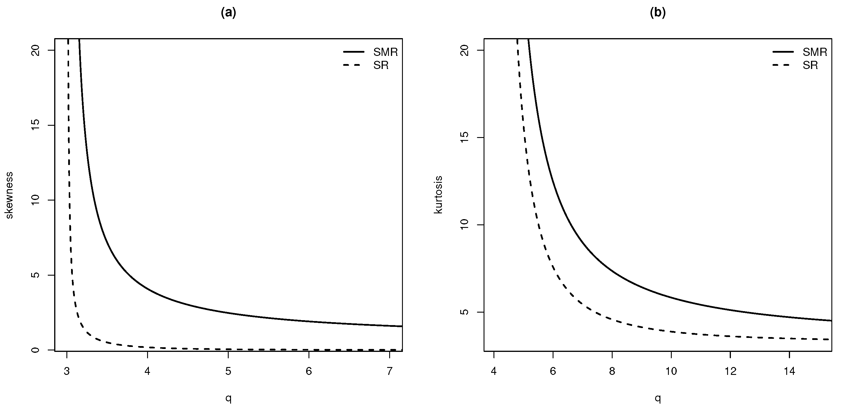
Note that the asymmetry and kurtosis coefficients only depend on the parameter q. Therefore q is a shape parameter since it determines the asymmetry and kurtosis coefficients of this model. In addition, it is of interest to compare both coefficients to other models, such as SR distribution, introduced in Iriarte et al. [10].
Figure 2 shows the plots for the asymmetry, (a), and kurtosis, (b), coefficients for SMR and SR models. We highlight that both coefficients are much higher for the SMR distribution than the ones for the SR model. That means that SMR distribution is more flexible with respect to the asymmetry and kurtosis than SR model.
To conclude, note that (9) and plot (a) in Figure 2 suggest that takes values in ; . On the other hand, (10) and plot (b) in Figure 2 suggest that approximately takes values in ; . That is, we are dealing with a skew right model, (the right tail is long relative to the left one), with positive kurtosis, i.e., heavy tails.
3. Lifetime Analysis
Since the SMR distribution is nonnegative and asymmetric, it can be used to model survival time data. In this section, the main features of interest in this field are studied. First the survival and hazard function for an SMR model are given.
Proposition 7.
Let with σ and . Then
- 1.
- The survival function is , .
- 2.
- The hazard function is
Proof.
Straightforward from and . □
Remark 4.
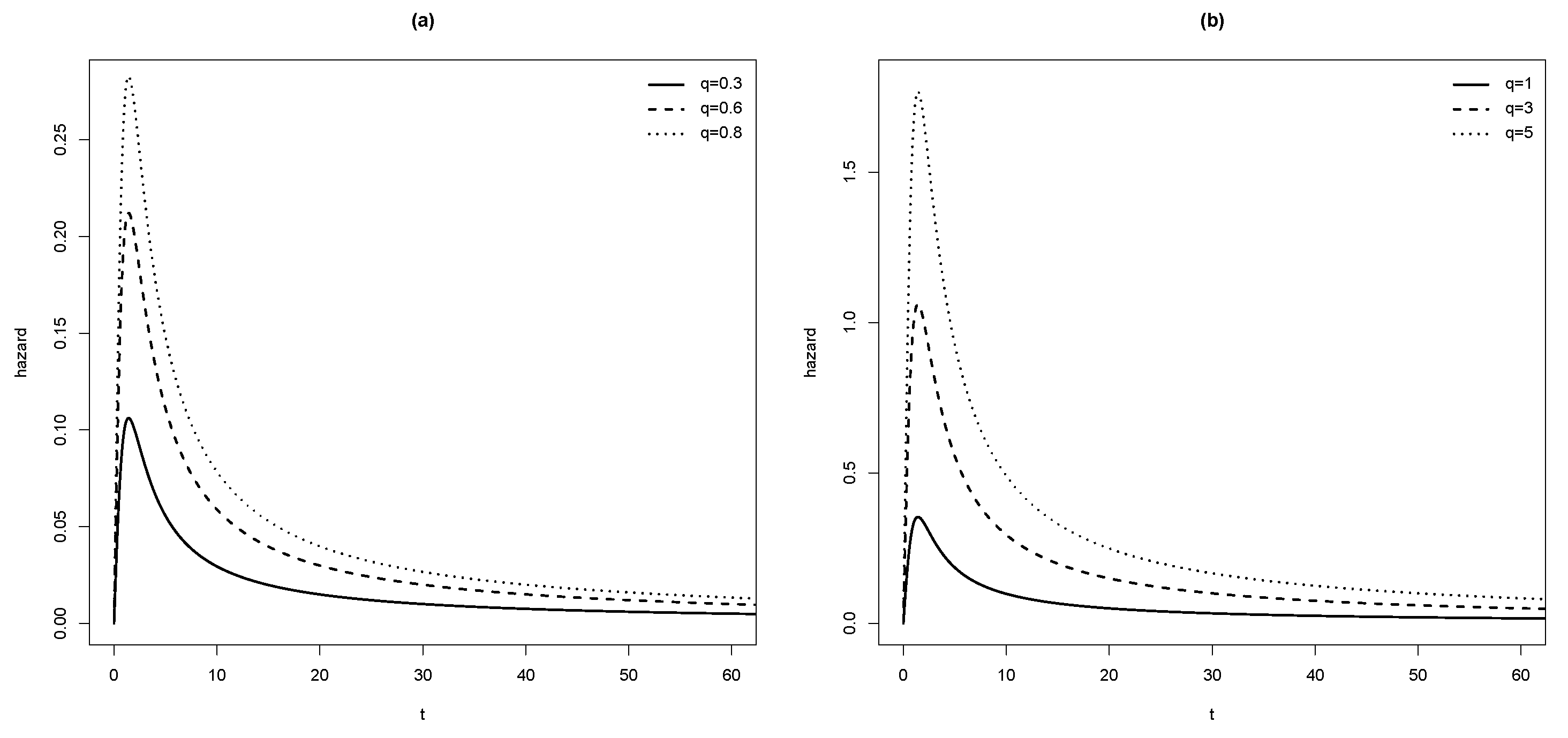
From (11), it follows that for an model the hazard function is monotone increasing for , monotone decreasing for and reaches its maximum at . Moroever,
Note that the intervals where is monotone only depend on the parameter σ, they do not depend on q.
Plots of are given in Figure 3 for and in (a) and in (b). In both settings, we note that the peak increases with q.
Remark 5.
For , the survival function of the SMR model satisfies that
Therefore, the survival function of the SMR distribution is regularly varying.
Mean Residual Life
Next the mean residual life is studied. Recall that for a nonnegative RV T, its mean residual life is defined as for . can be obtained as
with the survival function of T.
It will be proved that this characteristic can be expressed in terms of the survival function of a Pearson Type VII (PTVII) distribution.
Definition 3.
An RV W follows a PTVII distribution with parameters m, c and ξ (see Johnson et al. [17]) if its pdf is given by
with , , and . We denote as .
Proposition 8.
The mean residual life of , , can be obtained as
where denotes the survival function of an RV .
Proof.
Recall that
Note that the integrand in previous expression is, up to a constant, the pdf of a distribution. Therefore we can write
with the survival function of , . □
In Proposition 9, an explicit expression for (14) is given in terms of the regularized incomplete beta function, defined as
This expression is useful from a computational point of view.
Proposition 9.
For , the mean residual life of can be obtained as
Proof.
Let us consider the integral in (15) and the change of variable
Order Statistics
Given a random sample of size n of , let us denote by the order statistics, .
Proposition 10.
The pdf of is
In particular, the pdf of the minimum, , is
and the pdf of the maximum, , is
Proof.
Since we are dealing with an absolutely continuous model, the pdf of the order statistics is obtained by applying
where F and f denote the cdf and pdf of the parent distribution, in this case. □
Remark 6.
From (18), note that . That is, when sampling from an distribution then the minimum is also distributed according to an SMR model.
4. Entropy
In this section Rényi entropy is obtained for the SMR model. Given T an RV and , the Rényi entropy of T is given by
where denotes the Naperian logarithm.
Proposition 11.
Let and . Then the Rényi entropy of T is
5. Inference
In this section, moment and ML estimation methods are studied.
5.1. Moment Method Estimators
Let be a random sample from . Let us consider the first and second sample moments, denoted by and , respectively.
Proposition 12.
Given a random sample from with , the moment method estimators of σ and q are
where (23) must be solved numerically to obtain . Later, must be replaced in (22) to get .
5.2. ML Estimation
Let be a random sample from . Then the log-likelihood function is
Taking partial derivatives in with respect to and q and setting them equal to zero, we get
where (26) must be solved numerically to get , which must be substituted into (27) to obtain . Since we do not have explicit expressions for ML estimators, EM algorithm can be implemented to get these estimates. The next section is devoted to reach this aim.
5.3. ML Estimation Using EM-Algorithm
The EM-algorithm (Dempster et al. [18]) enables the computationally efficient determination of the ML estimates when iterative procedures are required. Next, details about the implementation of this algorithm for the SMR model are given. The method is based on Proposition 3 and Lemma 2.
Lemma 2.
Let with shape parameter and rate parameter, that is its pdf is , . Then
- 1.
- , , with pdf given in (2).
- 2.
- where denotes the digamma function.
Let , by applying the hierarchical representation given in Proposition 3, we can write and . The joint pdf of is
where Y is a latent variable and the parameter vector is , .
Given , a random sample of size n from , let us denote by the observed data, the unobserved data and the complete data, that is, the original data augmented by .
Let and the complete log-likelihood function associated with and its expected value, respectively. From (28), is
where c is a constant, which does not depend on .
In order to get and apply EM-algorithm, we need to calculate and . From (28) and (2)
where C is a constant that does not depend on . As (29) is related to the pdf of a Generalized Gamma distribution, specifically,
Then
On the other hand, Lemma 2 can be applied to (30) with
Taking into account that
we have
Let be the conditional expectation of the complete log-likelihood function. We have
with and given in (31) and (32), respectively. Taking first partial derivative with respect to , the estimate of is given by
where is the mean of . By proceeding similarly, the estimate of q is
where is the mean of and is the inverse of the digamma function. Therefore, the EM algorithm is
- E-step: For compute
- M-step: Update the vector of parameters
- E and M steps are repeated until a suitable convergence is reached.
EM algorithm implementation was carried out by using R software. Three functions were implemented. In the function used in E step, estimates of and were generated. In the function used in M step, estimates of and q were obtained. Later, these steps were repeated by using a function with the convergence criterion. The criterion was to stop when the difference between the successive values obtained is less than a a value fixed in advance, specifically it was
6. Simulation Study
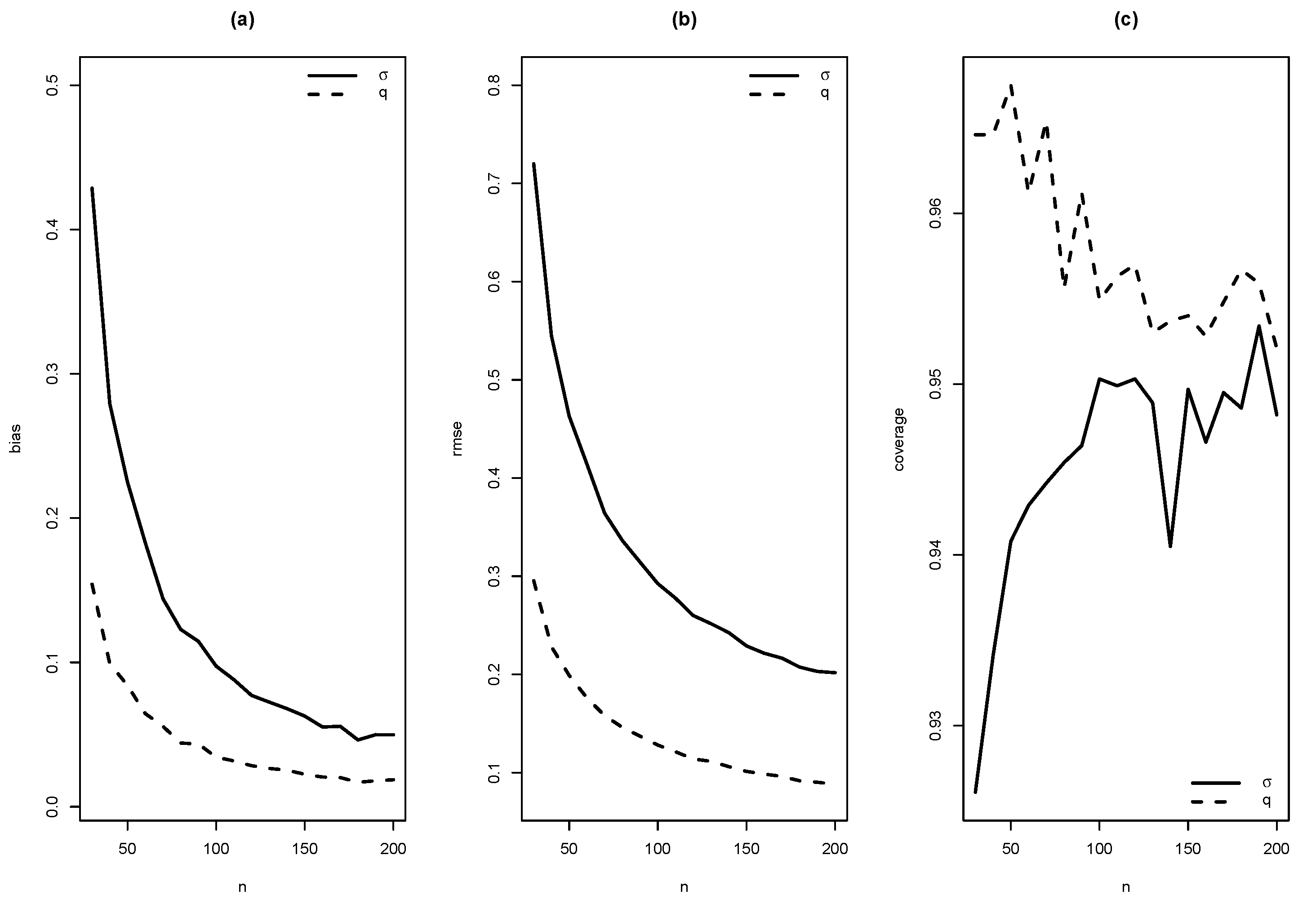
In this section, the performance of ML estimates for finite sample sizes is studied. It is empirically checked if the proposed estimators satisfy desirable properties, such as asymtotic unbiasedness, asymptotic efficiency, asymptotic normality. Values of the Rayleigh and the Generalized Gamma distributions were generated to get values of the SMR distribution introduced in (4). The EM algorithm was used to compute the estimates of parameters in the SMR model, and their standard errors. This procedure was carried out 10,000 times with sample sizes , and taking as values of the parameters 1 and 10; 1, 1.5, 2 and 3.
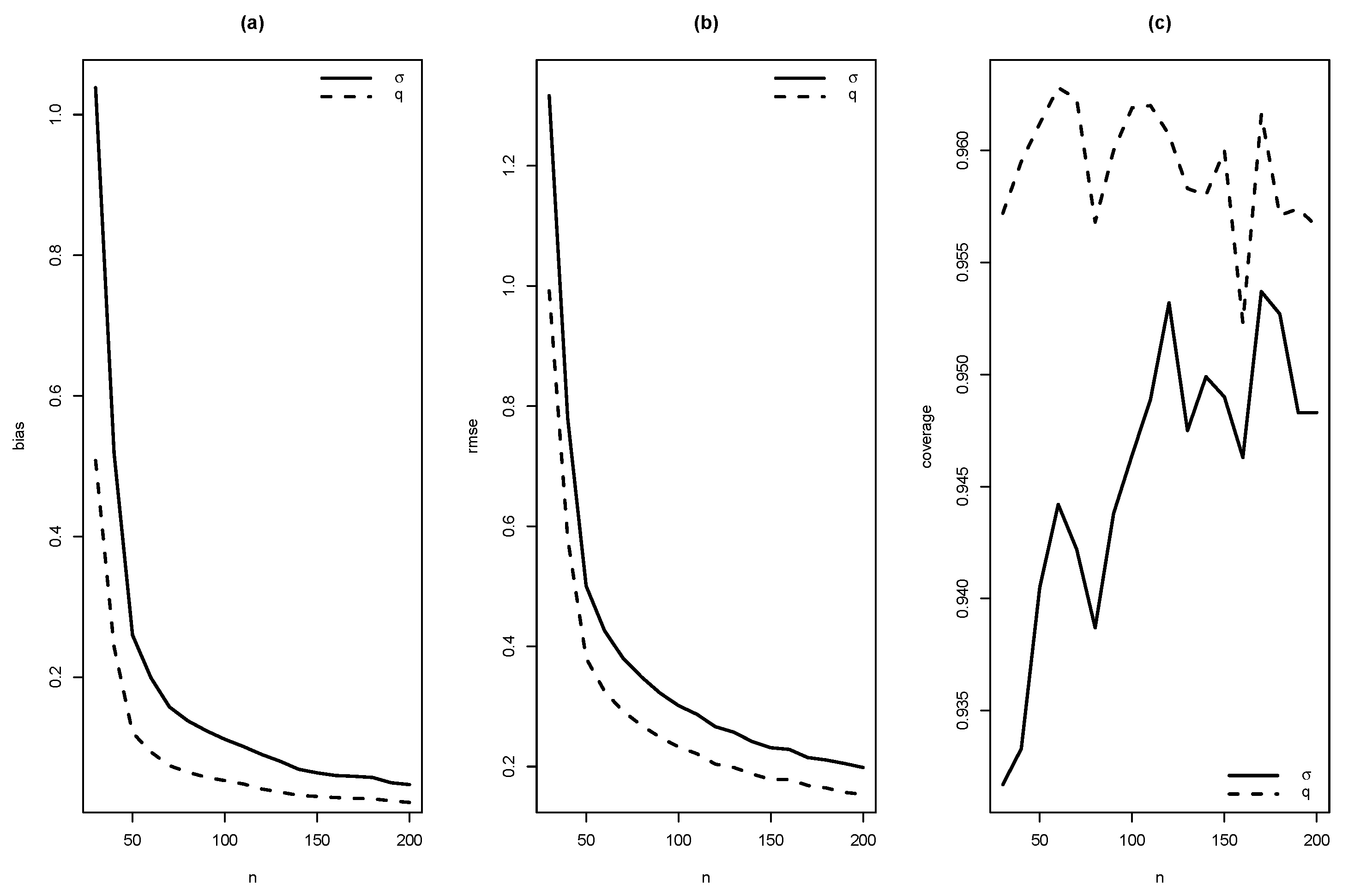
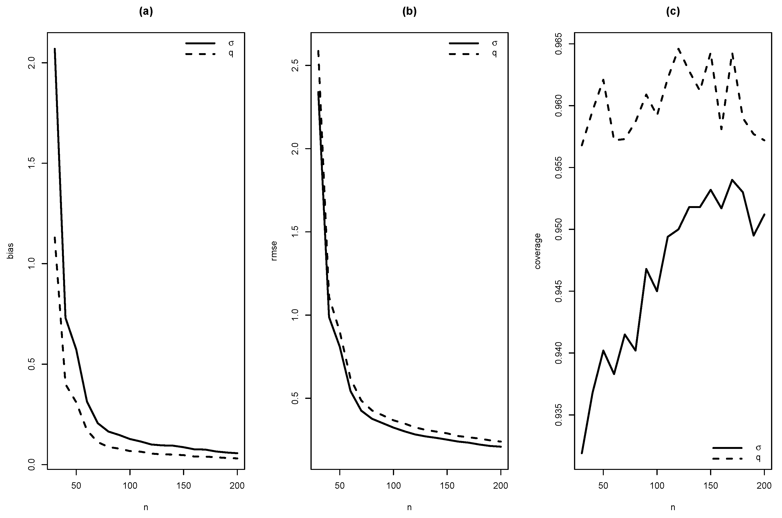
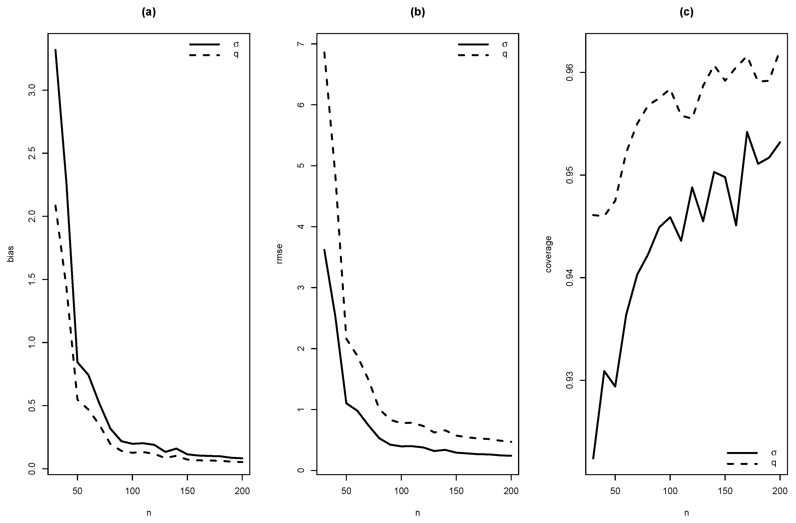
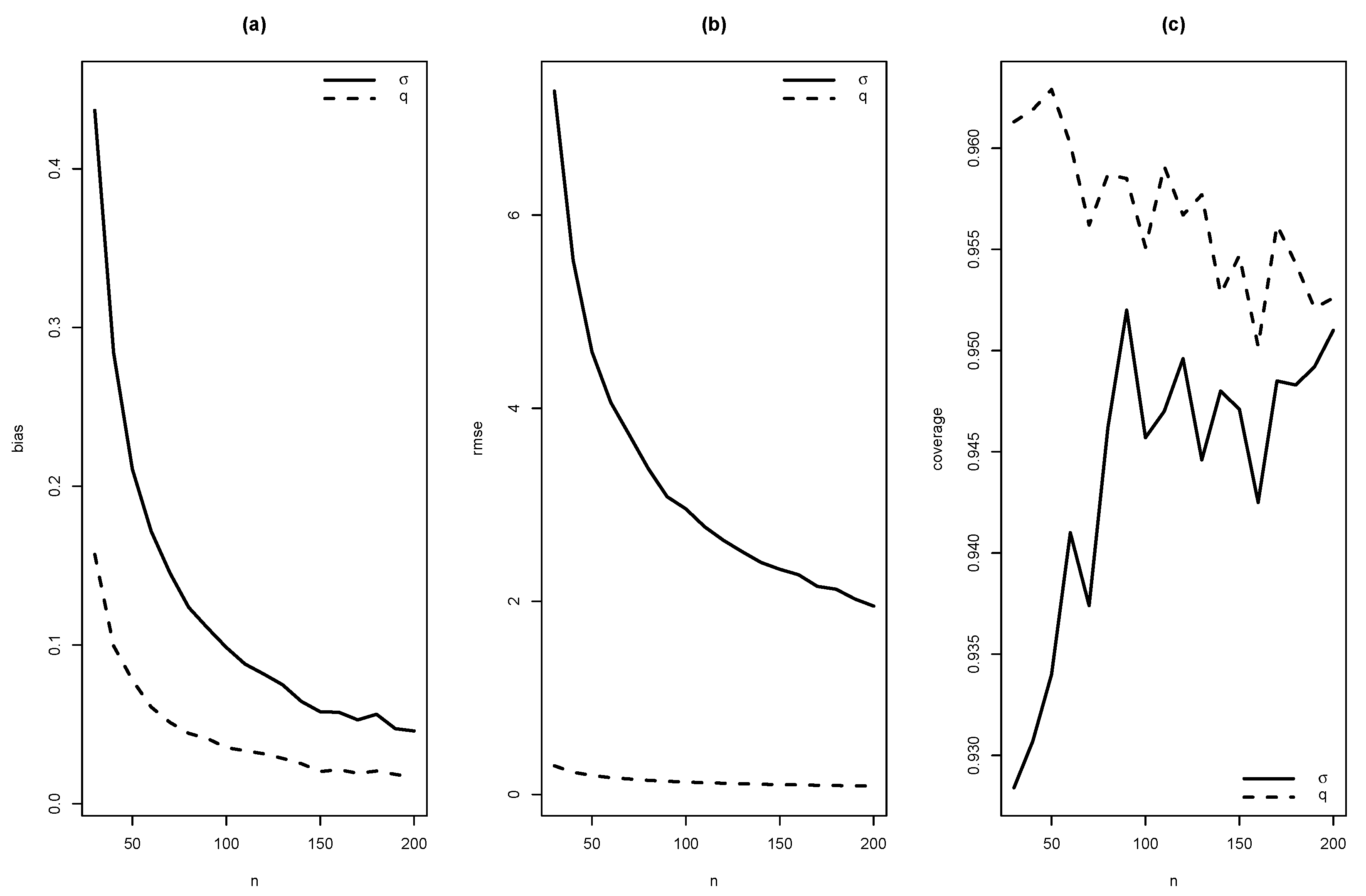
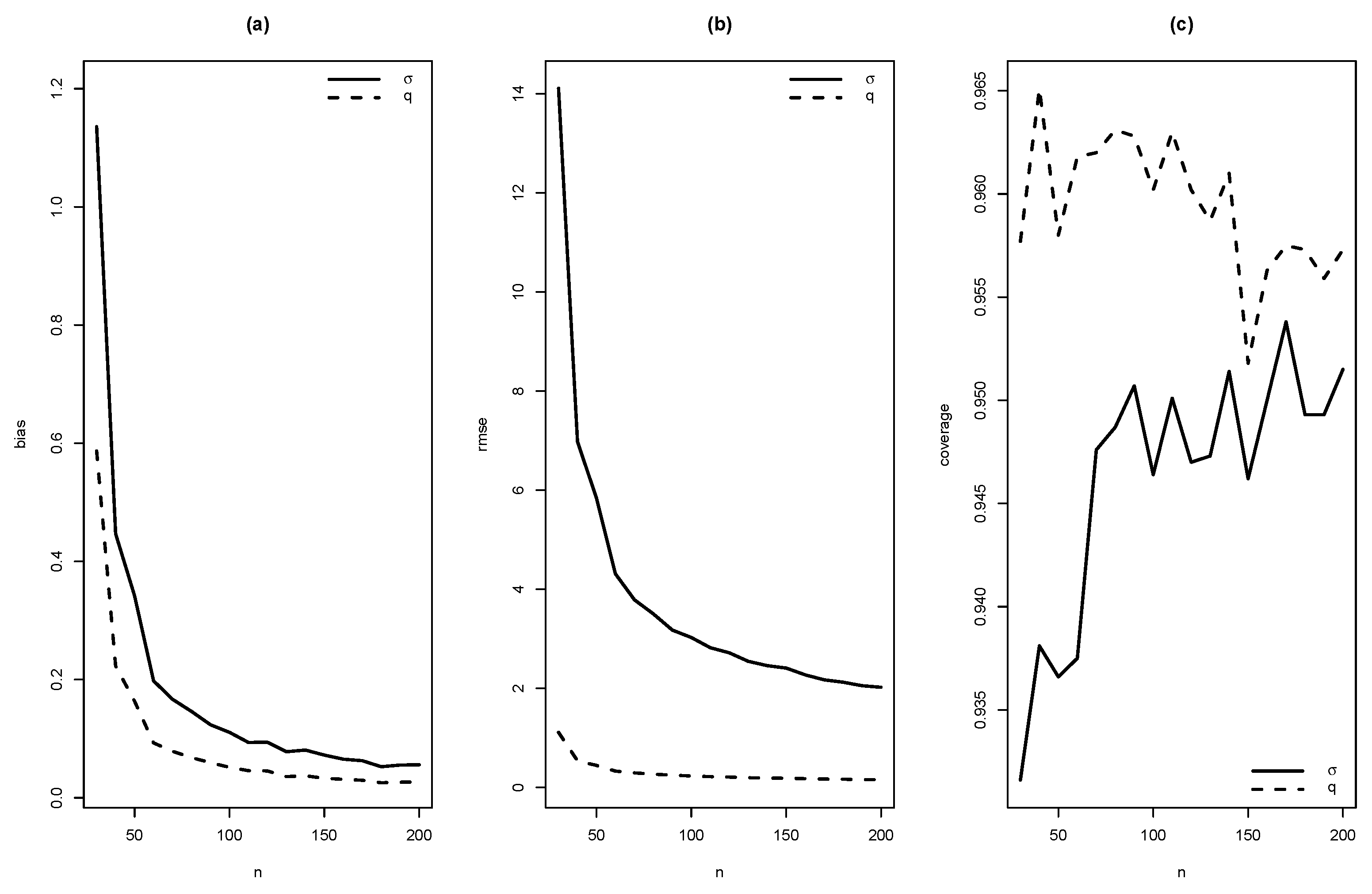
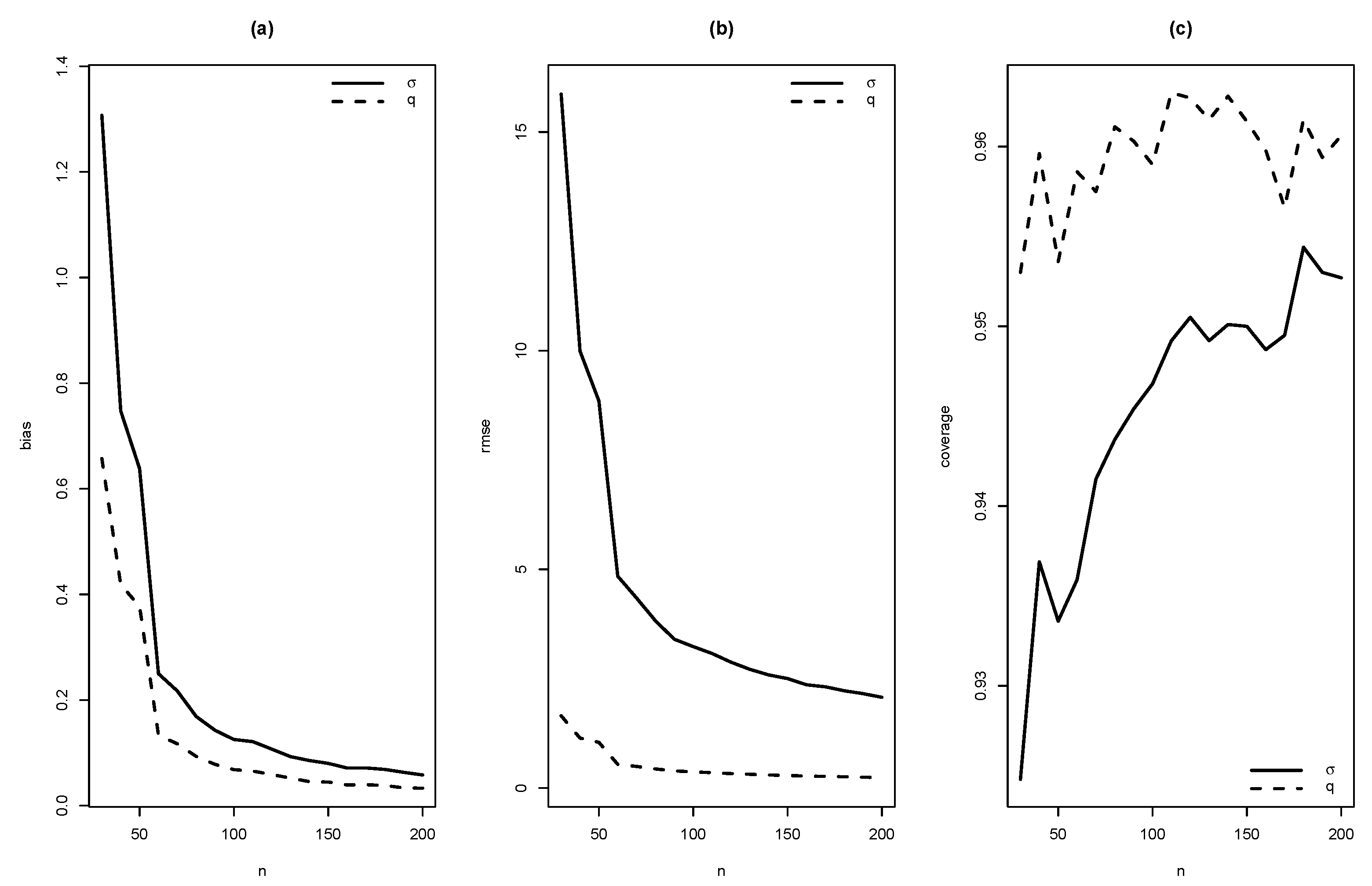
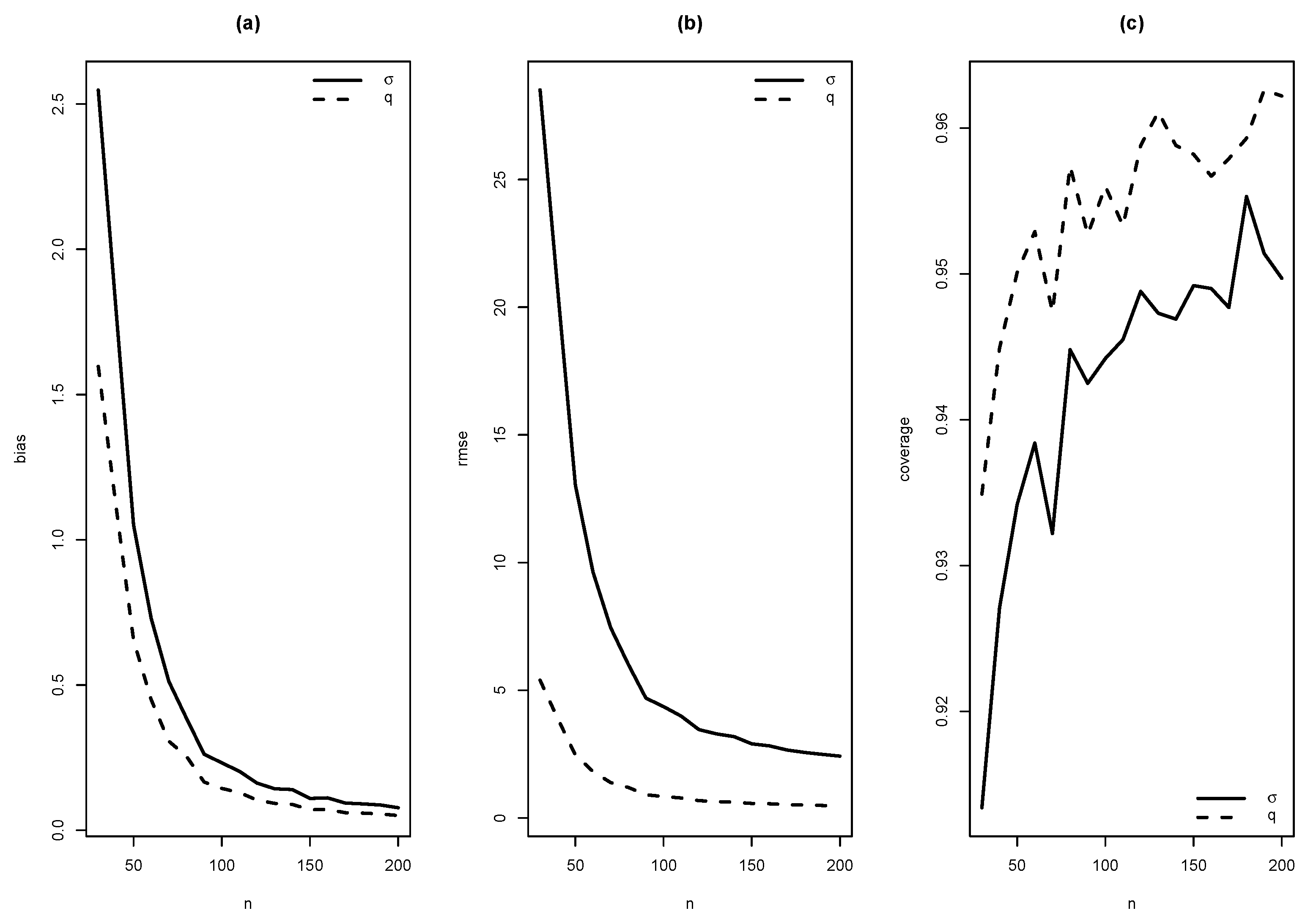
As summaries of these simulations, the average of estimates, average of standard errors of estimates, average bias, squared root of mean squared error (RMSE) and the empirical coverage probability of confidence intervals for the parameters (with confidence level 0.95) were calculated. From Figure 4, Figure 5, Figure 6, Figure 7, Figure 8, Figure 9, Figure 10 and Figure 11, average bias, RMSE and empirical coverage probability (in percentages) are plotted for n varying in . It is observed that if the sample size increases then bias and RMSE decrease, this fact suggests that the estimators are consistent. In addition, we note that the empirical coverage probability (in percentage) approaches to the nominal level (95%) when the sample size increases.
7. Real Data Illustration
In this section, we present applications of SMR model in two real datasets from the fields of lifetime analysis and reliability. To illustrate its good performance, our proposal is compared to other competing models previously introduced in literature. These are R and SR distributions.
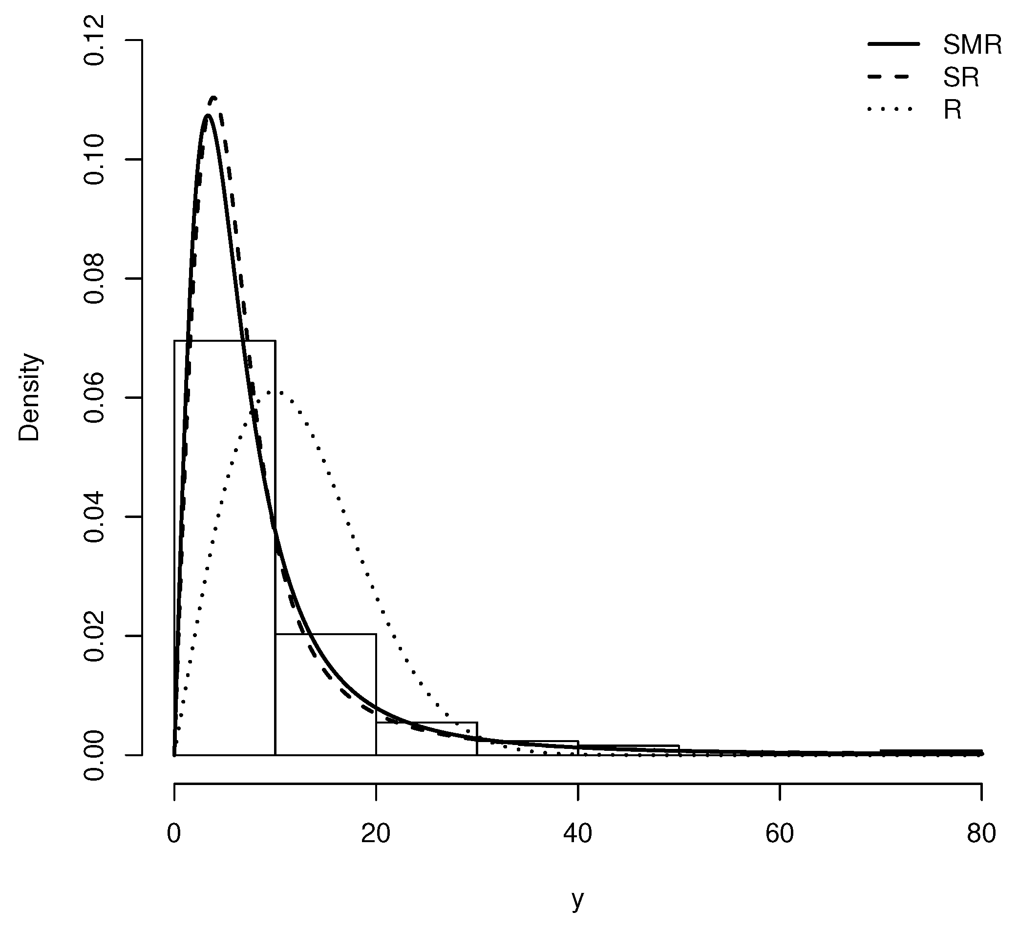
7.1. Application to Patients with Bladder Cancer
We consider a dataset corresponding to remission times (in months) of a random sample of 128 bladder cancer patients studied by Lee and Wang [19]. The model is proposed to describe this dataset. The EM algorithm was used to estimate and q. Their corresponding standard errors were obtained by using the inverse of the hessian matrix.
Table 1 provides the descriptive summaries. These are: the sample size n, the sample mean , the standard deviation S, the sample asymmetry coefficient , the sample kurtosis coefficient , the sample minimum and the sample maximum . We highlight that we are dealing with positive, positive skewed data with a really high kurtosis, .
Table 2 provides the ML estimates of parameters and their standard errors in parentheses for SMR, R and SR models. These models are compared by using the Akaike Information Criterion (AIC), Akaike [20] and the Bayesian Information Criterion (BIC), introduced in Schwarz [21]. Both criteria reveal that the SMR model provides a better fit to this data since their values are less than the others.
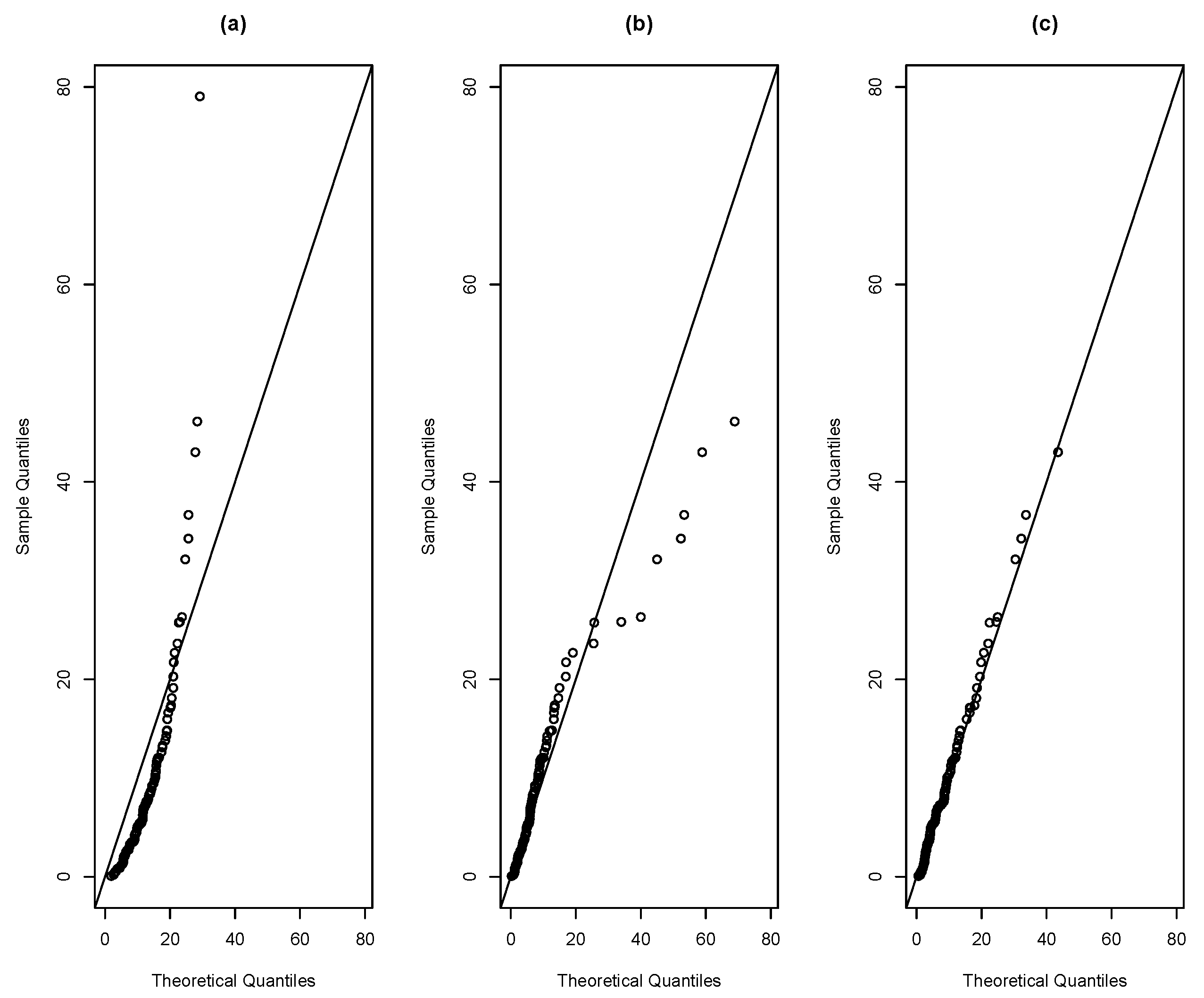
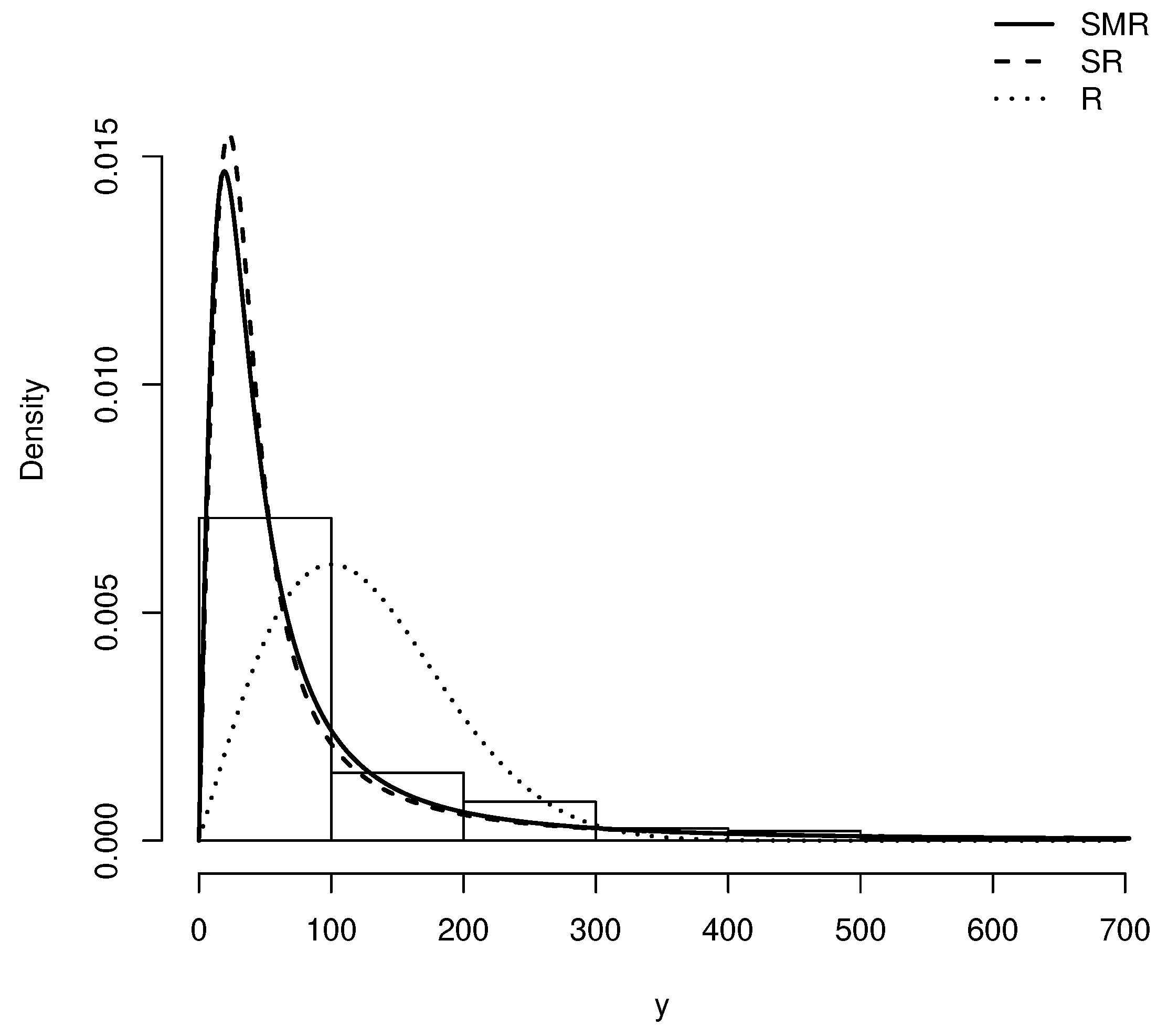
Figure 12 depicts the histogram of this dataset along with the estimated pdf for R, SR and SMR distributions. Moreover, Figure 13 provides the corresponding QQ-plots for these models. Note that the QQ-plots for R and SR models show that these distributions does not provide a good fit on the right tail of these data. However the QQ-plot for the SMR distribution does not exhibit this drawback.
All these plots and summaries suggest that the SMR model provides a better fit to this dataset than the other models under consideration.
7.2. Application to Number of Failures of an Air Conditioning System
The second dataset under consideration was reported by Proschan [22]. This dataset consists of the times between failures of the air-conditioning equipment in 13 Boeing 720 aircrafts. A similar outline to that given in previous applications has been followed. Table 3 shows the basic statistical summaries. We highlight that, again, a high value of kurtosis is observed .
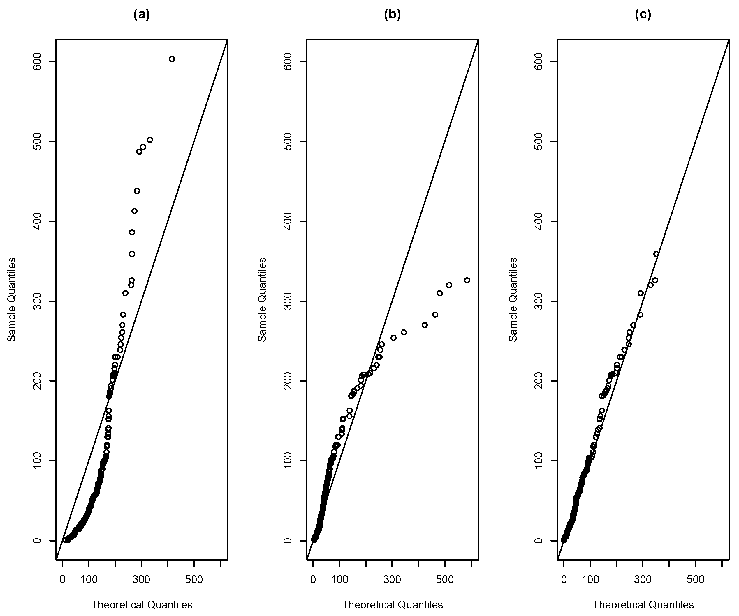
In Table 4, results related to the fit of R, SR and SMR models are given. Note that the SMR model provides a better fit over the others since its AIC and BIC values are less than those in R and SR models.
8. Conclusions
In this paper, the SMR distribution is introduced. As strengths of our proposal, we highlight that it is more flexible as for its kurtosis coefficient and hazard function than the Rayleigh and slashed Rayleigh distribution. Closed expressions are given for its main characteristics: pdf, cdf, moments and related coefficients. Since we are dealing with a positive and skew right model, it can be of interest for modeling survival time and reliability data. For this reason, features of interest in this field such as the hazard function, mean residual life and order statistics are studied. A closed expression is obtained for the Rényi entropy. The special interest is the EM estimation algorithm based on the hierarchical representation proposed for this model. A simulation study is included, which suggests that the ML estimators are consistent even for moderate sample sizes. Two real applications are included, in which AIC, BIC and QQ-plots show that our proposal provides a better fit than R and SR distributions, especially on the right tail of these datasets.
Author Contributions
Conceptualization, I.B.-C. and H.W.G.; formal analysis, P.A.R., I.B.-C., D.I.G. and H.W.G.; investigation, P.A.R., I.B.-C., D.I.G. and H.W.G.; methodology, I.B.-C. and H.W.G.; software, P.A.R. and D.I.G.; supervision, H.W.G.; validation, D.I.G. and I.B.-C.; visualization, H.W.G. All authors have read and agreed to the published version of the manuscript.
Funding
The research of I. Barranco-Chamorro was supported by Grant CTM2015-68276-R (Spain). The research of H.W. Gómez was supported by Grant SEMILLERO UA-2020 (Chile).
Conflicts of Interest
The authors declare no conflict of interest.
References
- Siddiqui, M.M. Some problems connected with Rayleigh distributions. J. Res. Natl. Bureu Stand. Ser. D 1962, 66, 167–174. [Google Scholar] [CrossRef]
- Miller, K.S. Multidimensional Gaussian Distributions; Wiley: New York, NY, USA, 1964. [Google Scholar]
- Polovko, A.M. Fundamentals of Reliability Theory; Academic Press: San Diego, CA, USA, 1968. [Google Scholar]
- Hirano, K. Rayleigh distribution, In Encyclopedia of Statistical Sciences; Kotz, S., Johnson, N.L., Read, C.B., Eds.; Wiley: New York, NY, USA, 1986; pp. 647–649. [Google Scholar]
- Lopez-Blazquez, J.F.; Barranco-Chamorro, I.; Moreno-Rebollo, J.L. Umvu estimation for certain family of exponential distributions. Commun. Stat.-Theory Methods 1997, 26, 469–482. [Google Scholar] [CrossRef]
- Ahmed, A.; Ahmad, S.P.; Reshi, J.A. Bayesian Analysis of Rayleigh Distribution. Int. J. Sci. Res. Publ. 2013, 3, 217–225. [Google Scholar]
- Sarti, A.; Corsi, C.; Mazzini, E.; Lamberti, C. Maximum likelihood segmentation of ultrasound images with Rayleigh distribution. IEEE Trans. Ultrason. Ferroelectr. Freq. Control 2005, 52, 947–960. [Google Scholar] [CrossRef] [PubMed] [Green Version]
- Kalaiselvi, S.; Loganathan, A.; Vijayaraghavan, R. Bayesian Reliability Sampling Plans under the Conditions of Rayleigh-Inverse-Rayleigh Distribution. Econ. Qual. Control 2014, 29, 29–38. [Google Scholar] [CrossRef]
- Dhaundiyal, A.; Singh, S.B. Approximations to the Non-Isothermal Distributed Activation Energy Model for Biomass Pyrolysis Using the Rayleigh Distribution. Acta Technol. Agric. 2017, 20, 78–84. [Google Scholar] [CrossRef] [Green Version]
- Iriarte, Y.A.; Gómez, H.W.; Varela, H.; Bolfarine, H. Slashed Rayleigh Distribution. Colomb. J. Stat. 2015, 38, 31–44. [Google Scholar] [CrossRef]
- Reyes, J.; Barranco-Chamorro, I.; Gallardo, D.; Gómez, H.W. Generalized modified slash Birnbaum-Saunders distribution. Symmetry 2018, 10, 724. [Google Scholar] [CrossRef] [Green Version]
- Reyes, J.; Barranco-Chamorro, I.; Gómez, H.W. Generalized modified slash distribution with applications. Commun. Stat.-Theory Methods 2020, 49, 2025–2048. [Google Scholar] [CrossRef]
- Iriarte, Y.A.; Varela, H.; Gómez, H.J.; Gómez, H.W. A Gamma-Type Distribution with Applications. Symmetry 2020, 12, 870. [Google Scholar] [CrossRef]
- Segovia, F.A.; Gómez, Y.M.; Venegas, O.; Gómez, H.W. A Power Maxwell Distribution with Heavy Tails and Applications. Mathematics 2020, 8, 1116. [Google Scholar] [CrossRef]
- Stacy, E.W. A generalization of the gamma distribution. Ann. Math. Stat. 1962, 33, 1187–1192. [Google Scholar] [CrossRef]
- Casella, G.; Berger, R.L. Statistical lnference; Duxbury Advanced Series; Thomson Learning: Pacific Grove, CA, USA, 2002. [Google Scholar]
- Johnson, N.L.; Kotz, S.; Balakrishnan, N. Continuous Univariate Distributions, 2nd ed.; Wiley Series in Probability and Statistics: New York, NY, USA, 1995; Volume 2. [Google Scholar]
- Dempster, A.P.; Laird, N.M.; Rubim, D.B. Maximum likelihood from incomplete data via the EM algorithm (with discussion). J. R. Stat. Soc. Ser. B 1977, 39, 1–38. [Google Scholar]
- Lee, E.T.; Wang, J. Statistical Methods for Survival Data Analysis; John Wiley & Sons: New York, NY, USA, 2003; Volume 476. [Google Scholar]
- Akaike, H. A new look at the statistical model identification. IEEE Trans. Autom. Control. 1974, 19, 716–723. [Google Scholar] [CrossRef]
- Schwarz, G. Estimating the dimension of a model. Ann. Stat. 1978, 6, 461–464. [Google Scholar] [CrossRef]
- Proschan, F. Theoretical explanation of observed decreasing failure rate. Technometrics 1963, 5, 375–383. [Google Scholar] [CrossRef]
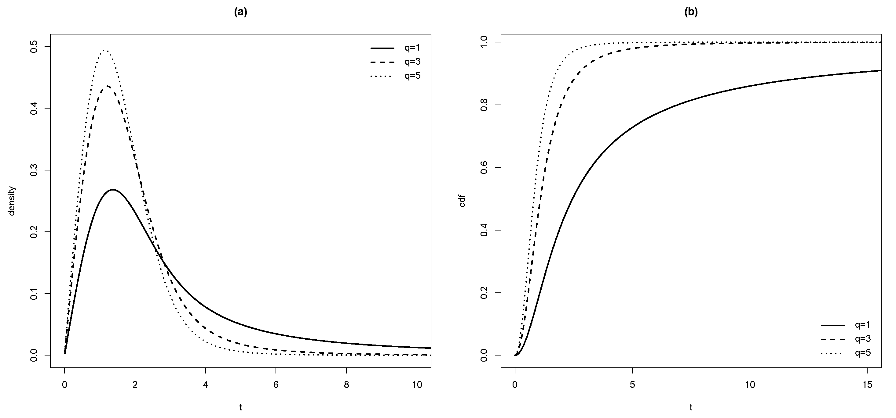
Figure 1.
(a) pdf and (b) cdf in SMR model for and different values of q.

Figure 2.
(a) Asymmetry and (b) kurtosis coefficients for the SMR and SR distribution.

Figure 3.
Hazard function model with (a) and (b) .

Figure 4.
Graphics of (a) bias, (b) RMSE and (c) coverage of simulation for , with .

Figure 5.
Graphics of (a) bias, (b) RMSE and (c) coverage of simulation for , 1.5 with .

Figure 6.
Graphics of (a) bias, (b) RMSE and (c) coverage of simulation for , with .

Figure 7.
Graphics of (a) bias, (b) RMSE and (c) coverage of simulation for , with .

Figure 8.
Graphics of (a) bias, (b) RMSE and (c) coverage of simulation for , with .

Figure 9.
Graphics of (a) bias, (b) RMSE and (c) coverage of simulation for , 1.5 with .

Figure 10.
Graphics of (a) bias, (b) RMSE and (c) coverage of simulation for , with .

Figure 11.
Graphics of (a) bias, (b) RMSE and (c) coverage of simulation for , with .

Figure 12.
Density adjusted for the remission times of patients with bladder cancer in the R, SR and SMR distributions.
Figure 12.
Density adjusted for the remission times of patients with bladder cancer in the R, SR and SMR distributions.

Figure 13.
QQ-plot for distributions (a) R, (b) SR, (c) SMR for the remission times of patients with bladder cancer.
Figure 13.
QQ-plot for distributions (a) R, (b) SR, (c) SMR for the remission times of patients with bladder cancer.

Figure 14.
Density adjusted for the number of failures of an air conditioning system in the R, SR and SMR distributions.
Figure 14.
Density adjusted for the number of failures of an air conditioning system in the R, SR and SMR distributions.

Figure 15.
QQ-plot for distributions (a) R, (b) SR, (c) SMR for the number of failures of an air conditioning system.
Figure 15.
QQ-plot for distributions (a) R, (b) SR, (c) SMR for the number of failures of an air conditioning system.


Table 1.
Descriptive statistics for the remission times of patients with bladder cancer.
| n | S | |||||
|---|---|---|---|---|---|---|
| 128 | 9.366 | 10.508 | 3.287 | 18.483 | 0.08 | 79.05 |
Table 2.
Estimates, standard errors (SE) in parenthesis, log-likelihood, AIC and BIC values for the remission times of patients with bladder cancer.
Table 2.
Estimates, standard errors (SE) in parenthesis, log-likelihood, AIC and BIC values for the remission times of patients with bladder cancer.
| Estimaciones | R (SE) | SR (SE) | SMR (SE) |
|---|---|---|---|
| 98.639 (8.718) | 8.647 (2.051) | 15.369 (5.108) | |
| - | 1.424 (0.224) | 1.772 (0.318) | |
| log-likelihood | −491.266 | −415.815 | −413.339 |
| AIC | 984.531 | 835.631 | 830.677 |
| BIC | 987.383 | 841.335 | 836.381 |
Table 3.
Descriptive statistics for number of failures of an air conditioning system.
| n | S | |||||
|---|---|---|---|---|---|---|
| 188 | 92.074 | 107.916 | 2.139 | 8.023 | 1 | 603 |
Table 4.
Estimates, SE in parenthesis, log-likelihood, AIC and BIC values for the number of failures of an air conditioning system.
Table 4.
Estimates, SE in parenthesis, log-likelihood, AIC and BIC values for the number of failures of an air conditioning system.
| Estimaciones | R (SE) | SR (SE) | SMR (SE) |
|---|---|---|---|
| 10,030.83 (730.135) | 264.611 (68.021) | 382.761 (113.843) | |
| - | 0.902 (0.107) | 1.069 (0.136) | |
| log-likelihood | −1191.275 | −1053.503 | −1046.549 |
| AIC | 2384.550 | 2111.006 | 2097.097 |
| BIC | 2387.787 | 2117.479 | 2103.570 |
Publisher’s Note: MDPI stays neutral with regard to jurisdictional claims in published maps and institutional affiliations. |
© 2020 by the authors. Licensee MDPI, Basel, Switzerland. This article is an open access article distributed under the terms and conditions of the Creative Commons Attribution (CC BY) license (http://creativecommons.org/licenses/by/4.0/).
Share and Cite
MDPI and ACS Style
Rivera, P.A.; Barranco-Chamorro, I.; Gallardo, D.I.; Gómez, H.W. Scale Mixture of Rayleigh Distribution. Mathematics 2020, 8, 1842. https://doi.org/10.3390/math8101842
AMA Style
Rivera PA, Barranco-Chamorro I, Gallardo DI, Gómez HW. Scale Mixture of Rayleigh Distribution. Mathematics. 2020; 8(10):1842. https://doi.org/10.3390/math8101842
Chicago/Turabian StyleRivera, Pilar A., Inmaculada Barranco-Chamorro, Diego I. Gallardo, and Héctor W. Gómez. 2020. "Scale Mixture of Rayleigh Distribution" Mathematics 8, no. 10: 1842. https://doi.org/10.3390/math8101842
Note that from the first issue of 2016, this journal uses article numbers instead of page numbers. See further details here.