Modeling of Strength Characteristics of Polymer Concrete Via the Wave Equation with a Fractional Derivative

Abstract

The article presents a solution to a boundary value problem for a wave equation containing a fractional derivative with respect to a spatial variable. This model is used to describe oscillation processes in a viscoelastic medium, in particular changes in the deformation-strength characteristics of polymer concrete (dian and dichloroanhydride-1,1-dichloro-2,2-diethylene) under the influence of the gravity force. Based on the obtained solution to the boundary value problem, the article presents four numerical examples corresponding to homogeneous boundary conditions and various initial conditions. The graphs of the found solutions were constructed and the calculation accuracy in the considered examples was estimated.

1. Introduction

Fractional calculus is currently at the center of attention of many researchers in the field of science and technology. In this regard, we should mention the monograph [1], which is a unique comprehensive review of fractional calculus and its application. Fractional partial differential equations play an increasingly important role in many fields of science and engineering, such as physics [2,3,4], biology [5,6], finance [7,8] and hydrodynamics [9,10]. Equations that contain fractional derivatives efficiently describe the motion of structures containing elastic and viscoelastic elements [11,12]. These equations also describe damped oscillations with fractional damping (in particular, the movement of rocks in earthquakes [13], fluctuation of nanoscale sensors, etc. [14,15]) and serve as a base for considering nonlinear oscillation processes [16]. The advantages of fractional derivatives are shown in modeling the mechanical and electrical properties of real materials, as well as in describing the rheological properties of rocks. Mathematical and simulation modeling of phenomena and processes, based on the description of their properties in terms of fractional derivatives, naturally leads to differential equations of fractional order.

Concrete structures are used everywhere in the construction of buildings and various structures since they are durable and reliable. At the same time, the concrete structure surface undergoes significant destructive effects because of external factors. Therefore, at present, based on a concrete mixture, a material with improved operating characteristics is being made—polymer concrete, which is distinguished by an increased, compared with concrete, resistance to moisture, low temperatures and chemical compounds and durability. Polymer concrete can be represented as a set of solid filler granules located in a viscoelastic medium in modeling. The transverse motion of a filler granule under the influence of the gravity force or an external force can be described by the equation of a fractional oscillator. Thus, replacing concrete with polymer concrete leads to replacing the second-order differential equation with a fractional-order differential equation.

Let us move on to the mathematical description.

2. Materials and Methods

We consider, in the domain $G=\left\{0\le x\le \mathfrak{X};0\le t\le 𝔍\right\}$, the first boundary value problem for the equation of string oscillation with a Riemann–Liouville fractional derivative of order α with respect to a spatial variable:

$$a^2\frac{{\partial }^{2}u}{\partial t^2}=\frac{{\partial }^{2}u}{\partial x^2}+c·D_{ox}^{\alpha }u.$$

(1)

Boundary conditions:

$$u\left(0,t\right)=u\left(\mathfrak{X},t\right)=0.$$

(2)

Initial conditions:

$$u\left(x,0\right)=\phi \left(x\right);$$

(3)

$$u_t^{\prime }\left(x,0\right)=\psi \left(x\right).$$

(4)

Here, 0 < α < 2—the order of the fractional derivative; c is a constant; the Riemann–Liouville fractional differential operator of order α > 0, where m − 1 < α ≤ m; m = 1,2, …, is defined as follows:

$$D_{ox}^{\alpha }f\left(x\right)=\frac{d^m}{d{x}^m}\left(\frac{1}{\mathsf{\Gamma }\left(m-\alpha \right)}{{\displaystyle \int }}_0^x\frac{f\left(\tau \right)d\tau }{{(x-\tau )}^{\alpha +1-m}}\right).$$

Assume that for functions (3)–(4), the following conditions hold:

$$\phi \left(x\right)\in C^2\left(0;\mathfrak{X}\right);{\phi }^{‴}\left(x\right)\in C\left(0;\mathfrak{X}\right);$$

(5)

$$\phi \left(0\right)=\phi \left(\mathfrak{X}\right)=0;$$

(6)

$${\phi }^{″}\left(0\right)={\phi }^{″}\left(\mathfrak{X}\right)=0;$$

(7)

$${\psi }^{″}\left(x\right)\in C\left(0;\mathfrak{X}\right);$$

(8)

$$\psi \left(0\right)=\psi \left(\mathfrak{X}\right)=0.$$

(9)

Note that more detailed information on Equation (1) can be found in [1]. Problems (1)–(4) are a generalization and refinement of the problem proposed in [17]. The results of [18] show that to simulate changes in the deformation-strength characteristics of polymer concrete under the influence of gravity force, one can use the result of solving problems (1)–(4). Samples of polymer concrete based on polyester resin (diane and diacyl chloride-1,1-dichloro-2,2-diethylene) were investigated. Polymer concrete is represented as a set of granules of mineral extender in an elastic-plastic medium. In this case, the motion of the granule u is described by Equation (1), where c—the viscosity modulus of the resin; a—related to the rigidity modulus of the resin; α—the elastic-plastic parameter of the medium. Let us show how to solve problems (1)–(4) by the Fourier method. Conditions (5)–(9) give us an opportunity to apply the Fourier method correctly in solving problems (1)–(4). Assume that

$$u\left(x,t\right)=X\left(x\right)T\left(t\right),$$

then for the unknown function X (x), we obtain the equality

$$X^{″}\left(x\right)+c·D_{ox}^{\alpha }X\left(x\right)=\lambda X\left(x\right).$$

(10)

Using the boundary conditions (2), we have:

$$X\left(0\right)=0;X\left(\mathfrak{X}\right)=0.$$

(11)

In this way, to find the unknown function $X\left(x\right)$, we obtain the two-point Dirichlet problem (10)–(11), whose solution, in the case 0 < α < 1, is given in [19].

It is a well-known fact [20] that a negative number λ is an eigenvalue of problems (10)–(11) if, and only if, λ is a zero of the function

$$\omega \left(\lambda \right)={\displaystyle \sum }_{n=0}^{\infty }{\left(-1\right)}^n{\displaystyle \sum }_{k=0}^n\frac{\left(\begin{array}{c}n\\ k\end{array}\right){\left(-\lambda \right)}^{n-k}{c}^k{\mathfrak{X}}^{2n+1-\mathrm{k}\mathsf{\alpha }}}{\mathsf{\Gamma }\left(2n+2-k\alpha \right)}.$$

(12)

The corresponding eigenfunctions $X_j\left(x\right)$ have the form

$$X_j\left(x\right)={{\displaystyle \sum }}_{n=0}^{\infty }{\left(-1\right)}^n{{\displaystyle \sum }}_{k=0}^n\frac{\left(\begin{array}{c}n\\ k\end{array}\right){\left(-{\lambda }_j\right)}^{n-k}{c}^k}{\mathsf{\Gamma }\left(2n+2-k\alpha \right)}{x}^{2n+1-k\alpha };j=1,2,3,\dots ;$$

(13)

here, ${\lambda }_j$ is j-th eigenvalue of problems (10)–(11). Here, the most important is the fact that the system of eigenfunctions (13) is complete in L₂ (see [20]).

Note that a general solution of the linear homogeneous equation

$$a^2{T}^{″}\left(t\right)={\lambda }_{m}T\left(t\right)$$

can be written as follows:

$$T_m\left(t\right)=A_m\sin \left(\frac{t}{a}\sqrt{-{\lambda }_m}\right)+B_m\cos \left(\frac{t}{a}\sqrt{-{\lambda }_m}\right).$$

Using this fact, we can write out the solution of the problems (1)–(4) in a standard form:

$$u\left(x,t\right)={\displaystyle \sum }_{m=1}^{\infty }{X}_m\left(x\right)T_m\left(t\right)$$

(14)

We will use the following form of initial condition (3)

$$u\left(x,0\right)={\displaystyle \sum }_{m=1}^{\infty }{X}_m\left(x\right)B_m=\phi \left(x\right)$$

(15)

and also use the following form of initial condition (4)

$$u{\prime }_t\left(x,0\right)={\displaystyle \sum }_{m=1}^{\infty }{A}_m{X}_m\left(x\right)\frac{\sqrt{-{\lambda }_m}}{a}=\psi \left(x\right).$$

(16)

The system of eigenfunctions (13) is complete but it is not orthogonal. Therefore, we introduce (according to [21]) the following system ${\left\{{\tilde{X}}_m\left(x\right)\right\}}_{m=1;2;\dots }$ of functions, which is biorthogonal to the considered-above system of eigenfunctions.

$${\tilde{X}}_m\left(x\right)={{\displaystyle \sum }}_{n=0}^{\infty }{\left(-1\right)}^n{{\displaystyle \sum }}_{k=0}^n\frac{\left(\begin{array}{c}n\\ k\end{array}\right){\left(-{\lambda }_m\right)}^{n-k}{c}^k}{\mathsf{\Gamma }\left(2n+2-k\alpha \right)}{\left(\mathfrak{X}-x\right)}^{2n+1-k\alpha };m=1,2,3,\dots$$

(17)

Now, it is possible to obtain a system of equations from Equations (15) and (16) for finding the coefficients ${\left\{A_m\right\}}_{m=1}^M$ and ${\left\{B_m\right\}}_{m=1}^M$. Multiplying both sides of (15) and (16) scalarly, we obtain

$$\{\begin{array}{c}\langle {\tilde{X}}_m\left(x\right),X_m\left(x\right)\rangle B_m=\langle \phi \left(x\right),{\tilde{X}}_m\left(x\right)\rangle \\ \langle {\tilde{X}}_m\left(x\right),X_m\left(x\right)\rangle A_m\frac{\sqrt{-{\lambda }_m}}{a}=\langle \psi \left(x\right),{\tilde{X}}_m\left(x\right)\rangle \end{array};m=1;2;\dots$$

where

$$\langle f\left(x\right),g\left(x\right)\rangle =\underset{0}{\overset{\mathfrak{X}}{{\displaystyle \int }}}f\left(x\right)·g\left(x\right)dx.$$

It follows that

$$\{\begin{array}{c}{B}_m=\frac{\langle \phi \left(x\right),{\tilde{X}}_m\left(x\right)\rangle }{\langle {\tilde{X}}_m,X_m\rangle }\\ A_m=\frac{a\langle \psi \left(x\right),{\tilde{X}}_m\left(x\right)\rangle }{\sqrt{-{\lambda }_m}\langle {\tilde{X}}_m\left(x\right),X_m\left(x\right)\rangle }\end{array};m=1;2;\dots$$

(18)

Note that due to the fulfillment of conditions (5)–(9), we conclude that the series corresponding to the functions $u\left(x,t\right)$, $\frac{{\partial }^{2}u}{\partial t^2}$ and $\frac{{\partial }^{2}u}{\partial x^2}$ converge uniformly (see [22]).

3. Results

Let us find, numerically, the first eigenvalues and the corresponding eigenfunctions (using the partial sum of the series in (12) and (13)) via the multi-paradigm numerical computing environment MATLAB. Considering a model of the polymer concrete reaction under the influence of the gravity force, we have the following notations: α—parameter of viscoelasticity of a medium; c—viscosity modulus of a medium. It is a known fact (see [23]) that for the polymer concrete based on polyester resin (dian and dichloroanhydride-1,1-dichloro-2,2-diethylene), we have α = 1.47 and c = 1.8.

The first seven eigenvalues corresponding to α = 1.47, c = 1.8 and $\mathfrak{X}=1$ are given in

Table 1. The first seven eigenvalues of boundary value problems (10)–(11) for α = 1.47, c = 1.8 and $\mathfrak{X}=1$.

λ1	λ2	λ3	λ4	λ5	λ6	λ7
−16.51	−59.49	−125.13	−213.33	−323.27	−455.09	−607.31

.

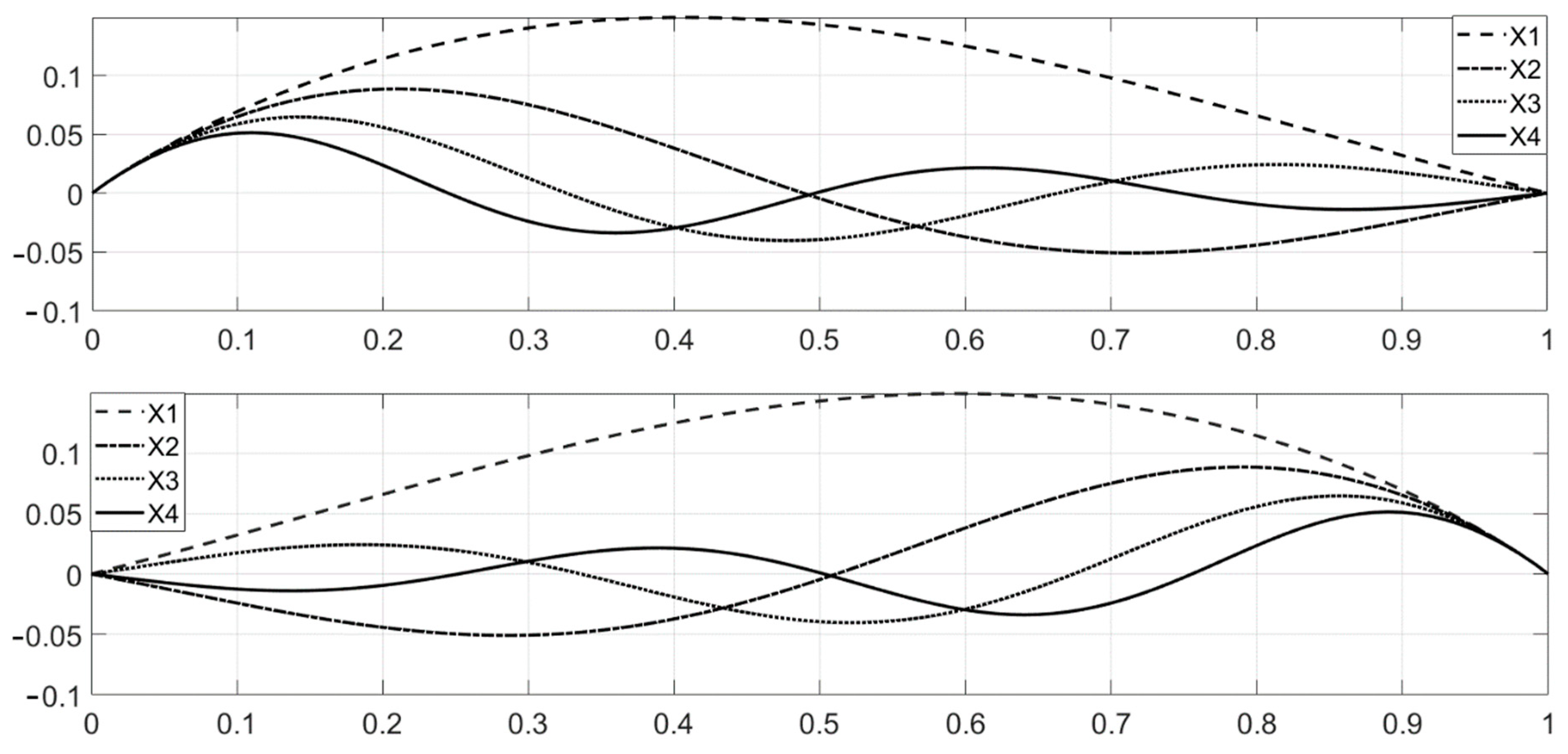
The seven eigenfunctions ${\left\{X_m\left(x\right)\right\}}_{m=1;2;\dots 7}$ and the functions from the biorthogonal system ${\left\{{\tilde{X}}_m\left(x\right)\right\}}_{m=1;2;\dots 7}$ have been obtained numerically, due to formulas (13) and (17), by replacing the series with the partial sums of the first 100 terms. The first four eigenfunctions, of the system ${\left\{X_m\left(x\right)\right\}}_{m=1;2;\dots },$ corresponding to the case α = 1.47, c = 1.8 and $\mathfrak{X}=1$ are shown at the top of Figure 1, and the first four, of the system ${\left\{{\tilde{X}}_m\left(x\right)\right\}}_{m=1;2;\dots },$ corresponding to the same case are at the bottom of Figure 1.

Further, using the MATLAB high-level language for technical calculations, we calculated the values of the inner product $\langle {\tilde{X}}_k\left(x\right),X_m\left(x\right)\rangle$ for the first seven functions of both systems and wrote out the results in

Table 2. Inner product of the first seven eigenfunctions of boundary value problems (10)–(11) and functions of the biorthogonal system; α = 1.47, c = 1.8 and $\mathfrak{X}=1$.

$\langle {\tilde{\mathit{X}}}_{\mathit{k}},{\mathit{X}}_{\mathit{m}}\rangle$	${\mathit{X}}_1$	${\mathit{X}}_2$	${\mathit{X}}_3$	${\mathit{X}}_4$	${\mathit{X}}_5$	${\mathit{X}}_6$	${\mathit{X}}_7$
${\tilde{X}}_1$	0.01046	0	0	0	0	0	0
${\tilde{X}}_2$	0	−0.00213	0	0	0	0	0
${\tilde{X}}_3$	0	0	0.00076	0	0	0	0
${\tilde{X}}_4$	0	0	0	−0.00035	0	0	0
${\tilde{X}}_5$	0	0	0	0	0.00018	0	0
${\tilde{X}}_6$	0	0	0	0	0	−0.00011	0
${\tilde{X}}_7$	0	0	0	0	0	0	0.00007

with an accuracy of five decimal places.

The matrix of the inner product is diagonal, thus the numerically-found systems of functions ${\left\{X_m\left(x\right)\right\}}_{m=1;2;\dots }$ and ${\left\{{\tilde{X}}_m\left(x\right)\right\}}_{m=1;2;\dots }$ are biorthogonal at the given level of accuracy.

Now, let us consider examples and find an approximate solution to problems (1)–(4) using, instead of expressing, a solution in the form of series (14), the sum of the first seven terms

$$u_{\left(7\right)}\left(x,t\right)={\displaystyle \sum }_{m=1}^7{X}_m\left(x\right)T_m\left(t\right).$$

In Examples 1–4, the function $\phi \left(x\right)$ determines the initial position of the granules of the mineral filler and the function $\psi \left(x\right)$ determines the initial speed of the granules of the mineral filler.

Example 1.

Let $\mathfrak{X}=1;𝔍=3;\phi \left(x\right)=0;\psi \left(x\right)=x{\left(1-x\right)}^2$. To solve problems (1)–(4), using system (12), we find the values of the first seven coefficients $A_m$ and $B_m$ in series (14). The values of coefficients $A_m$, calculated by virtue of (18), are shown in

Table 3. The values of the coefficients $A_m$ of the solution $u_{\left(7\right)}\left(x,t\right)$ (see Example 1).

$\mathit{m}$	1	2	3	4	5	6	7
$A_m$	0.20862	0.05574	−0.01698	0.01228	−0.00812	0.00586	−0.00503

.

$$B_m=0;m=1;2;\dots 7$$

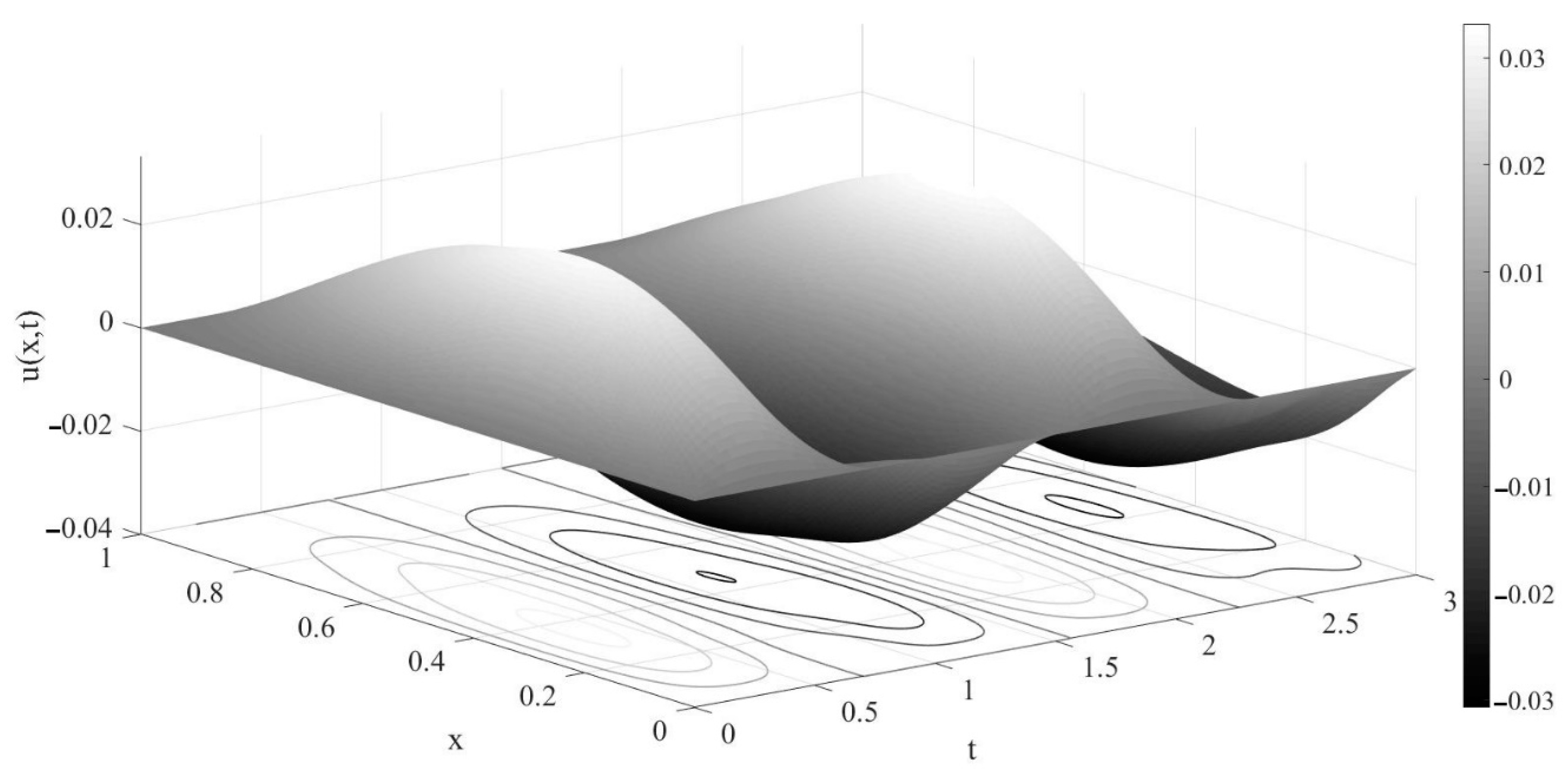
The graph of the approximate solution $u_{\left(7\right)}\left(x,t\right)$ is shown in Figure 2.

Let us estimate how much the last (seventh) term contributes to the sum; for this purpose, we consider the ratio of the variation of the seventh term to the variation of the sum of the first seven terms:

$$\frac{max\left\{X_7\left(x\right)T_7\left(t\right)\right\}-min\left\{X_7\left(x\right)T_7\left(t\right)\right\}}{max\left\{u_{\left(7\right)}\left(x,t\right)\right\}-min\left\{u_{\left(7\right)}\left(x,t\right)\right\}}100\%=0.5\%$$

Let us indicate the upper estimate for the series members (14):

$$\left|X_m\left(x\right)T_m\left(t\right)\right|\le 0.03·m^{-2.8}.$$

Example 2.

Let $\mathfrak{X}=1;𝔍=4;\phi \left(x\right)=0;\psi \left(x\right)=\left(1-x\right)x^3$. To solve problems (1)–(4), using system (12), we find the values of the first seven coefficients $A_m$ and $B_m$ in series (14). The values of coefficients $A_m$, calculated by virtue of (18), are shown in

Table 4. The values of coefficients $A_m$ and $B_m$ of the solution $u_{\left(7\right)}\left(x,t\right)$ (see Example 2).

$\mathit{m}$	1	2	3	4	5	6	7
$A_m$	0.14149	−0.13295	0.07009	−0.04226	0.02925	−0.02173	0.01719

.

$$B_m=0;m=1;2;\dots 7$$

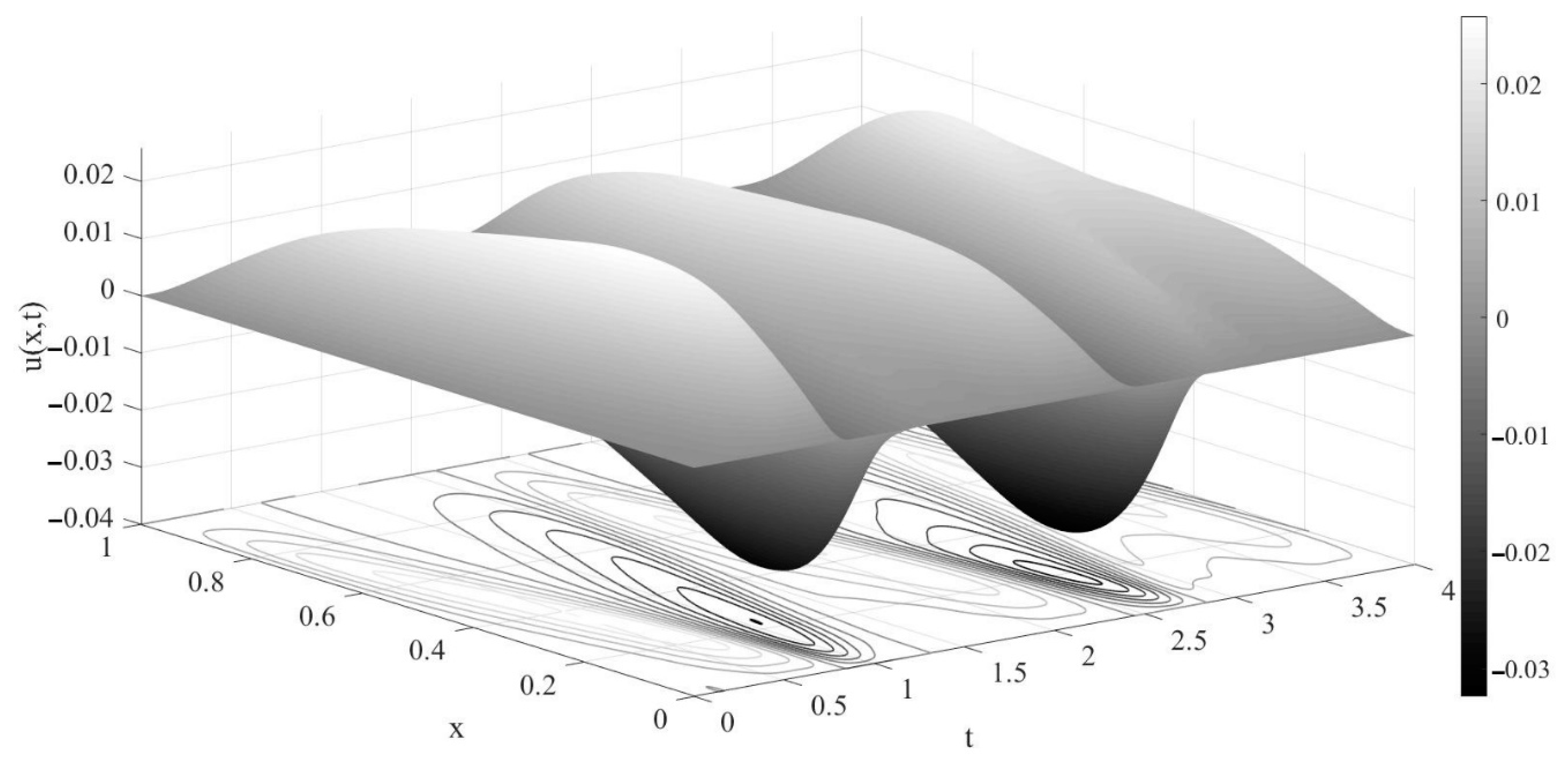
The graph of the approximate solution $u_{\left(7\right)}\left(x,t\right)$ is shown in Figure 3.

Let us estimate how much the last (seventh) term contributes to the sum; for this purpose, we consider the ratio of the variation of seventh term to the variation of sum of the first seven terms:

$$\frac{max\left\{X_7\left(x\right)T_7\left(t\right)\right\}-min\left\{X_7\left(x\right)T_7\left(t\right)\right\}}{max\left\{u_{\left(7\right)}\left(x,t\right)\right\}-min\left\{u_{\left(7\right)}\left(x,t\right)\right\}}100\%=1.9\%.$$

Let us indicate the upper estimate for the series members (14):

$$\left|X_m\left(x\right)T_m\left(t\right)\right|\le 0.07·m^{-2.5}.$$

Example 3.

Let $\mathfrak{X}=1;𝔍=5;\phi \left(x\right)=x\left(1-x\right);\psi \left(x\right)=x{\left(1-x\right)}^4$. To solve problems (1)–(4), using system (12), we find the values of the first seven coefficients $A_m$ and $B_m$ in series (14). The values of coefficients $A_m{\mathrm{and}B}_m,$ calculated by virtue of (18), are shown in

Table 5. The values of the coefficients $A_m$ and $B_m$ of the solution $u_{\left(7\right)}\left(x,t\right)$ (see Example 3).

$\mathit{m}$	1	2	3	4	5	6	7
$A_m$	0.06758	0.05946	0.01514	0.00500	0.00236	0.00120	0.00049
$B_m$	1.81104	−0.70356	0.38444	−0.33961	0.23810	−0.24218	0.18670

.

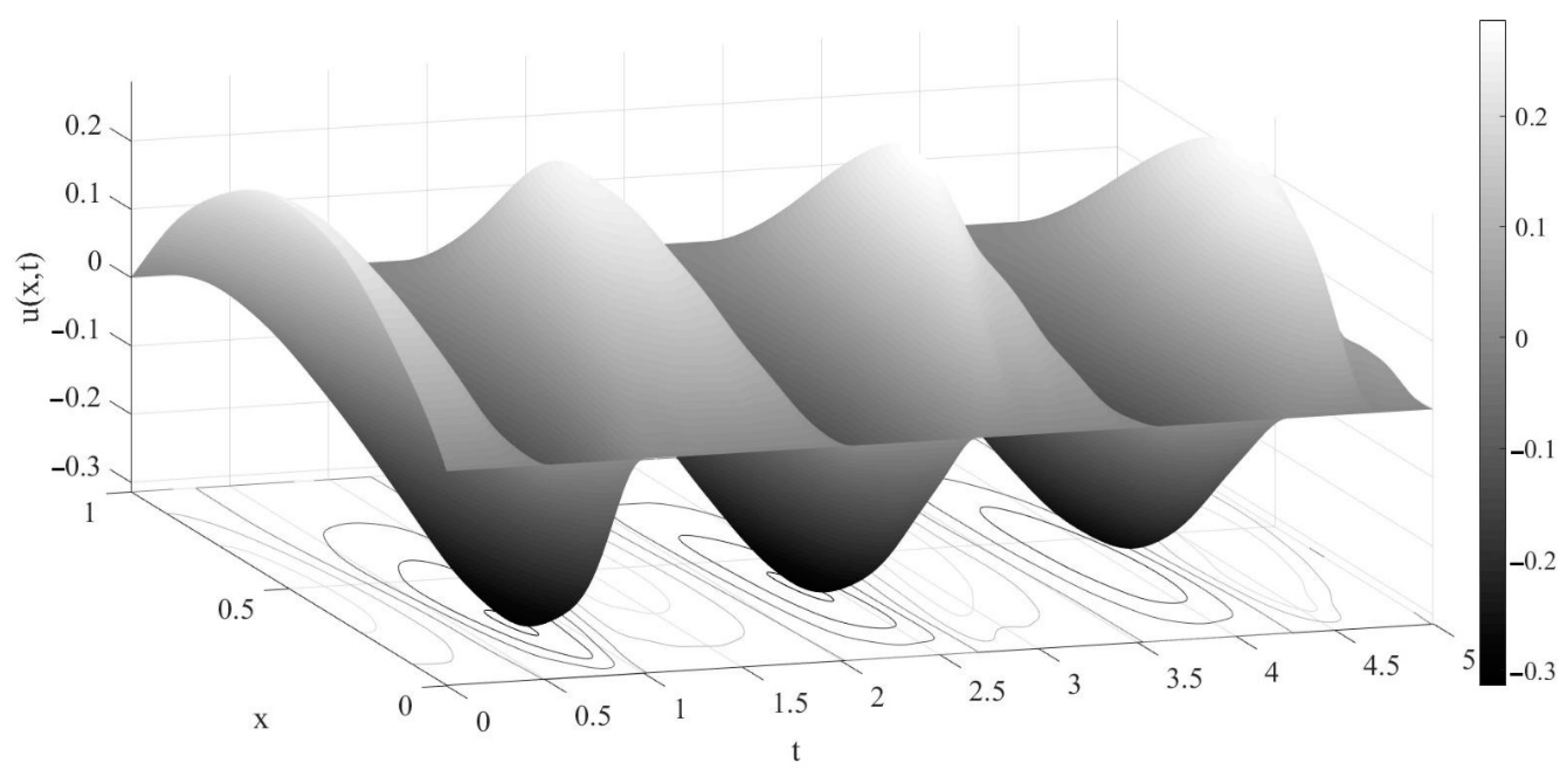
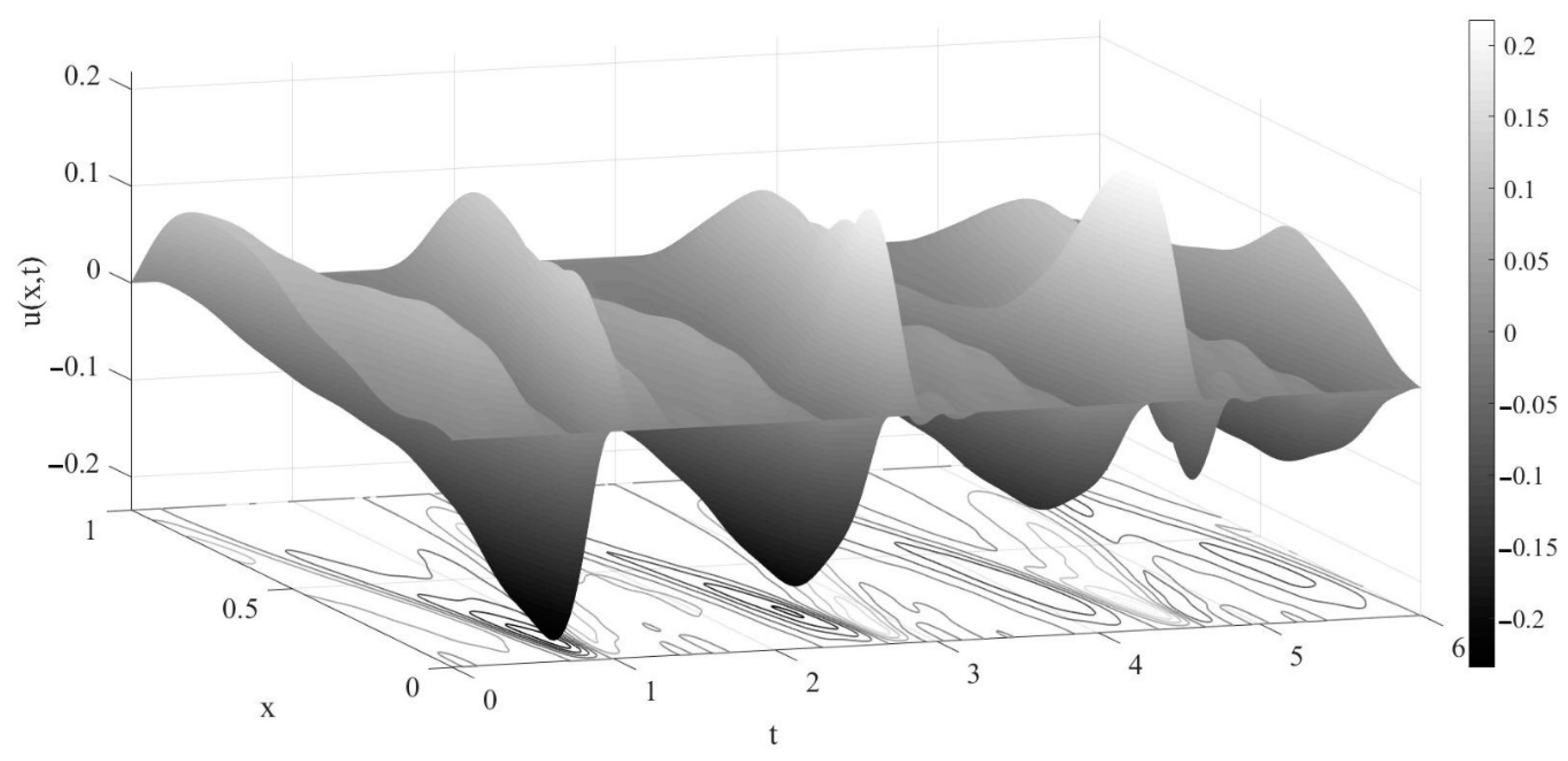
The graph of the approximate solution $u_{\left(7\right)}\left(x,t\right)$ is shown in Figure 4.

Let us estimate how much the last (seventh) term contributes to the sum; for this purpose, we consider the ratio of the variation of seventh term to the variation of sum of the first seven terms:

$$\frac{max\left\{X_7\left(x\right)T_7\left(t\right)\right\}-min\left\{X_7\left(x\right)T_7\left(t\right)\right\}}{max\left\{u_{\left(7\right)}\left(x,t\right)\right\}-min\left\{u_{\left(7\right)}\left(x,t\right)\right\}}100\%=2.0\%.$$

Let us indicate the upper estimate for the series members (14):

$$\left|X_m\left(x\right)T_m\left(t\right)\right|\le 0.27·m^{-2.1}.$$

Example 4.

Let $\mathfrak{X}=1;𝔍=6;\phi \left(x\right)=\left(1-x\right)x^3;\psi \left(x\right)=\left(1-x\right)x^3$. To solve problems (1)–(4), using system (12), we find the values of the first seven coefficients $A_m$ and $B_m$ in series (14). The values of coefficients $A_m{\mathrm{and}B}_m,$ calculated by virtue of (18), are shown in

Table 6. The values of the coefficients $A_m$ and $B_m$ of the solution $u_{\left(7\right)}\left(x,t\right)$ (see Example 4).

$\mathit{m}$	1	2	3	4	5	6	7
$A_m$	0.14149	−0.13295	0.07009	−0.04226	0.02925	−0.02173	0.01719
$B_m$	0.57490	−1.02545	0.78405	−0.61730	0.52588	−0.46347	0.42359

.

The graph of the approximate solution $u_{\left(7\right)}\left(x,t\right)$ is shown in Figure 5.

Let us estimate how much the last (seventh) term contributes to the sum; for this purpose, we consider the ratio of the variation of seventh term to the variation of sum of the first seven terms:

$$\frac{max\left\{X_7\left(x\right)T_7\left(t\right)\right\}-min\left\{X_7\left(x\right)T_7\left(t\right)\right\}}{max\left\{u_{\left(7\right)}\left(x,t\right)\right\}-min\left\{u_{\left(7\right)}\left(x,t\right)\right\}}100\%=6.0\%.$$

Let us indicate the upper estimate for the series members (14):

$$\left|X_m\left(x\right)T_m\left(t\right)\right|\le 0.29·m^{-1.6}.$$

4. Discussion

In this article:

-

The solution to problems (1)–(4) is presented.

-

The first seven eigenvalues of problems (10)–(11) are found in the case α = 1.47; c = 1.8; $\mathfrak{X}=1$, which gives us an opportunity to model the deformation-strength characteristics of polymer concrete (dian and dichloroanhydride-1,1-dichloro-2,2-diethylene) under the influence of the gravity force, with an accuracy of two decimal places.

-

The functions from the system ${\left\{{\tilde{X}}_m\left(x\right)\right\}}_{m=1;2;\dots }$, which is biorthogonal to the system of eigenfunctions ${\left\{X_m\left(x\right)\right\}}_{m=1;2;\dots }$ of problems (10)–(11), in the case α = 1.47; c = 1.8; $\mathfrak{X}=1$, are found numerically and their graphs are plotted.

-

The inner products of the eigenfunctions ${\left\{X_m\left(x\right)\right\}}_{m=1;2;\dots }$ of problems (10)–(11) and functions from the biorthogonal system ${\left\{{\tilde{X}}_m\left(x\right)\right\}}_{m=1;2;\dots },$ in the case α = 1.47; c = 1.8; $\mathfrak{X}=1$, are calculated and the obtained result confirms the correctness of replacing series (13) and (17) with partial sums in the calculations.

-

Four numerical examples of the application of the solution to problems (1)–(4) to modeling changes in the deformation-strength characteristics of polymer concrete (dian and dichloroanhydride-1,1-dichloro-2,2-diethylene) under the influence of the gravity force are considered.

-

The rate of decrease in terms (14) corresponding to the considered examples is obtained:

$$\left|X_m\left(x\right)T_m\left(t\right)\right|\le C·m^{\gamma },$$

where

$$0<C<0.3;-3<\gamma <-1.5$$

-

In the considered-above examples, we have established that the seventh (last) term contributes to the sum from 0.5% to 6%.

This allows us to speak about the sufficient accuracy of using seven terms to model changes in the deformation-strength characteristics of polymer concrete (dian and dichloroanhydride-1,1-dichloro-2,2-diethylene) under the influence of the gravity force.

References

- Handbook of Fractional Calculus with Applications; Tenreiro, J.A.; De Gruyter, M. (Eds.) GmbH: Berlin, Germany; Boston, MA, USA, 2019; Volume 1–8. [Google Scholar]
- Herrmann, R. Fractional Calculus: An Introduction for Physicists, 2nd ed.; World Scientific: Singapore, 2014. [Google Scholar]
- Sandev, T.; Tomovshi, Z. Fractional Equations and Models: Theory and Applications; Springer: Berlin/Heidelberg, Germany, 2019. [Google Scholar]
- Zaslavsky, G.M. Chaos, fractional kinetics, and anomalous transport. Phys. Rep. 2002, 371, 461–580. [Google Scholar] [CrossRef]
- Magin, R.L. Fractional Calculus in Bioengineering; Begell House: New York, NY, USA; Danbury, CT, USA, 2006. [Google Scholar]
- Yuste, S.B.; Lindenberg, K. Subdiffusion-limited reactions. Chem. Phys. 2002, 284, 169–180. [Google Scholar] [CrossRef] [Green Version]
- Sabatelli, L.; Keating, S.; Dudley, J.; Richmond, P. Waiting time distributions in financial markets. Eur. Phys. J. B 2002, 27, 273–275. [Google Scholar] [CrossRef]
- Song, L.; Wang, W. Solution of the fractional Black-Scholes option pricing model by finite difference method. Abstr. Appl. Anal. 2013, 45, 1–16. [Google Scholar] [CrossRef] [Green Version]
- Aleroev, T.S.; Aleroeva, H.T.; Huang, J.F.; Nie, N.M.; Tang, Y.F.; Zhang, S.Y. Features of seepage of a liquid to a chink in the cracked deformable layer. Int. J. Model. Simul. Sci. Comput. 2010, 1, 333–347. [Google Scholar] [CrossRef]
- Jiang, X.; Yu, X.M. Analysis of fractional anomalous diffusion caused by an instantaneous point source in disordered fractal media. Int. J. Non-Lin. Mech. 2006, 41, 156–165. [Google Scholar]
- Chirkii, A.A.; Matichin, I.I. On linear conflict-controlled processes with fractional derivatives. Tr. Inst. Mat. Mekh. UrO RAN 2011, 17, 256–270. [Google Scholar]
- Ingman, D.; Suzdalnitsky, J. Control of damping oscillations by fractional differential operator with time-dependent order. Comput. Methods Appl. Mech. Eng. 2004, 193, 5585–5595. [Google Scholar] [CrossRef]
- Koh, G.K.; Kelly, J. Application of fractional derivatives to seismic analysis of base-isolated models. Earthq. Eng. Struct. Dyn. 1990, 19, 229–241. [Google Scholar] [CrossRef]
- Draganescu, G.E.; Cofan, N.; Rujan, D.L. Nonlinear vibrations of a nano-sized sensor with fractional damping. J. Optoelectron. Adv. Mater. 2005, 7, 877–884. [Google Scholar]
- Fenlander, A. Modal synthesis when modeling damping by use of fractional derivatives. AIAA J. 1996, 34, 1051–1058. [Google Scholar] [CrossRef]
- Meilanov, R.P.; Yanpolov, M.S. Features of the phase trajectory of a fractal oscillator. Tech. Phys. Lett. 2002, 28, 30–32. [Google Scholar] [CrossRef]
- Aleroev, T. The analysis of the polymer concrete characteristics by fractional calculus. Phys. Conf. Ser. Modeling Methods Struct. Anal. 2019, 1425, 012112. [Google Scholar] [CrossRef] [Green Version]
- Aleroev, T.; Erokhin, S.; Kekharsaeva, E. Modeling of deformation-strength characteristics of polymer concrete using fractional calculus. IOP Mater. Sci. Eng. 2018, 365, 032004. [Google Scholar] [CrossRef] [Green Version]
- Aleroev, T.S.; Kekharsaeva, E. Boundary Value Problems for Differential Equations with Fractional Derivatives. Integral Transform. Spec. Funct. 2017, 28, 900–908. [Google Scholar] [CrossRef]
- Aleroev, T.; Aleroeva, H. Problems of Sturm-Liouville type for differential equations with fractional derivatives. In Fractional Differential Equations; Kochubei, A., Luchko, Y., Eds.; De Gruyter: Berlin, Germany; Boston, MA, USA, 2019; pp. 21–46. [Google Scholar]
- Aleroev, T.S.; Kirane, M.; Tang, Y.F. Boundary-value problems for differential equations of fractional order. J. Math Sci. 2013, 10, 158–175. [Google Scholar] [CrossRef] [Green Version]
- Samarskiy, A.A.; Tikhonov, A.N. Equations of Mathematical Physics: Textbook, 6th ed.; Publishing house of Moscow State University: Moscow, Russia, 1999; pp. 82–96. [Google Scholar]
- Aleroev, T.; Kirianova, L. Presence of Basic Oscillatory Properties in the Bagley-Torvik Model. In IPICSE-2018 MATEC Web of Conferences; EDP Sciences: Les Ulis, France, 2018; Volume 251, p. 04022. [Google Scholar]
Figure 1.
The first four functions, of the system , (at the top) and (at the bottom), corresponding to the case α = 1.47 and c = 1.8.
Figure 2.
The graph of the approximate solution of problems (1)–(4) under the imposed conditions in Example 1.
Figure 3.
A graph of the approximate solution of problems (1)–(4) under the imposed conditions in Example 2.
Figure 4.
A graph of the approximate solution of problems (1)–(4) under the imposed conditions in Example 3.
Figure 5.
A graph of the approximate solution of problems (1)–(4) under the imposed conditions in Example 4.