Reinforcement-Learning Based Dynamic Transmission Range Adjustment in Medium Access Control for Underwater Wireless Sensor Networks


1
Computer Science, The City University of New York -The Graduate Center, 365 5th Ave, New York, NY 10016, USA
2
Computer Science, The City College of New York, 160 Convent Ave, New York, NY 10031, USA
3
Electrical & Computer Engineering, Mississippi State University, Mississippi State, MS 39762, USA
4
Computer Science, University of Alabama, Tuscaloosa, AL 35487, USA
*
Author to whom correspondence should be addressed.
Electronics 2020, 9(10), 1727; https://doi.org/10.3390/electronics9101727
Submission received: 13 September 2020
/
Revised: 30 September 2020
/
Accepted: 9 October 2020
/
Published: 20 October 2020
(This article belongs to the Special Issue Underwater Communication and Networking Systems)
Abstract
:In this paper, we propose a reinforcement learning (RL) based Medium Access Control (MAC) protocol with dynamic transmission range control (TRC). This protocol provides an adaptive, multi-hop, energy-efficient solution for communication in underwater sensors networks. It features a contention-based TRC scheme with a reactive multi-hop transmission. The protocol has the ability to adjust to network conditions using RL-based learning algorithm. The combination of TRC and RL algorithms can hit a balance between the energy consumption and network performance. Moreover, the proposed adaptive mechanism for relay-selection provides better network utilization and energy-efficiency over time, comparing to existing solutions. Using a straightforward ALOHA-based channel access alongside “helper-relays” (intermediate nodes), the protocol is able to obtain a substantial amount of energy savings, achieving up to 90% of the theoretical “best possible” energy efficiency. In addition, the protocol shows a significant advantage in MAC layer performance, such as network throughput and end-to-end delay.
1. Introduction
Covering approximately 70% of the Earth’s surface, the oceans are one of the most important natural resources on this planet. The vast but largely unexplored oceans have been the center of a global competition for the riches of the world’s final frontier [1]. In the past decade, Underwater Wireless Sensor Network (UWSN) emerges as the enabling technology for applications such as environment monitoring, aquatic data collection, undersea explorations and exploitation, hence attracting much attention from both the industry and academia.
While we are exploring ever deeper into the blue oceans, more and more underwater sensors and instruments are being deployed. As a result, the oceans are becoming surprisingly noisy and crowded [2]. Looking forward, we envision that future UWSN systems could evolve into an Internet of Underwater Things (IoUT) [3], hosting a wide variety of intelligent underwater devices, such as smart underwater sensors, advanced telemetry instruments, high precision underwater positioning systems, USBL- based tracking devices, and much more. Each of these devices would have underwater communication capability, thus forming a densely deployed network at locations of interest.
For such a network to operate efficiently, two major research challenges will have to be addressed. The first challenge is how to design an effective medium access control (MAC) protocol for the network nodes to share a common wireless channel when there are multiple neighbors in the transmission range. Since electro-magnetic waves do not work well in water, UWSN often adopts acoustic signals to carry information. Acoustic waves travel at 1500 m/s in water, which is five orders of magnitude slower than the speed of electro-magnetic signals in terrestrial wireless communications. This leads to a significantly long propagation delay. Consequently, conventional handshaking based MAC protocols will experience a performance degradation, as the round trip time increases significantly [4]. Further, carrier-sensing based MAC protocols become less efficient in UWSN because a busy local channel does not necessarily indicate a busy channel at a remote network node [4]. Therefore, a new method needs to be designed in order to improve the network throughput and reduce the number of packet collisions.
The second challenge is the energy consumption. On the one hand, acoustic communication is known to be energy hungry. For example, the WHOI micro-modem, a well-known underwater acoustic modem, needs 150 W of power in transmission mode [5], whereas the TR1000 module for RF communications only takes 48 mW when in transmission mode [6]. As a result, in UWSN, the energy efficiency of the wireless network design can affect the overall system performance considerably. On the other hand, underwater sensors are mostly battery powered, with limited capacity. Replacing batteries in the field can be a logistical nightmare. Therefore, it is critical to improve the energy efficiency when designing UWSNs, especially for applications that require a long system life time.
In this paper, we propose a MAC protocol, called Learning Based Transmission Range Adjustment (LIBRA) to tackle these two challenges. First, we acknowledge the fact that the path loss is non-linear, and the power consumption grows rapidly with the increase of distance [7]. Instead of transmitting at the maximum range to reach a one-hop neighbor, we design the protocol to employ intermediate nodes to forward packets towards the destination within the source node’s maximum transmission range. Second, reducing transmission range can also be used as a way to reduce the number of packet collisions. This is because a reduced transmission range means a reduced interference range, leading to a reduced number of packet collisions. As a result, more network nodes can share the same channel, allowing concurrent transmissions possible within the network, hence boosting the overall network throughput. Third, a reinforcement learning algorithm is designed for selecting the proper intermediate nodes, i.e., relays, for the best energy saving. This is a very important feature for the highly dynamic ocean environment. Lastly, an ALOHA type scheme with implicit acknowledgement is developed for the transmissions between relays. ALOHA is known for its insensitivity to long propagation delays in the underwater environment [8,9,10]. Therefore its performance will not be penalized when the propagation delay increases in an UWSN, e.g., when network size grows or the next hop moves away from the previous node.
LIBRA can be considered as a crossover between MAC and network protocols. On the one hand, like a MAC protocol, it handles the data transfer between adjacent network nodes within their transmission range, i.e., single hop. On the other hand, for a one-hop destination, LIBRA tries to transmit the packet through multiple relays to save energy. Note that LIBRA is not a cross layer design since the route discovery and routing decision to a remote destination are handled independently by the routing protocol, and LIBRA does not require the cross-layer collaboration with a routing protocol. This design can make LIBRA compatible with a variety of routing protocols, which can optimize for different aspects of the network performance. As a result, the network will be able to meet a diverse and complicated user needs.
The contributions of the paper are: (1) we introduce a novel method to improve the energy efficiency in UWSN by employing relays to achieve good energy efficiency with minimum control message overhead; (2) we present and investigate a reinforcement learning based forwarding mechanism, conventionally a network layer service, into MAC layer; (3) we evaluate the benefits and overheads of employing multiple relays within a single-hop collision domain.
The rest of the paper is organized as follows: In Section 2, we present the related work. In Section 3, we describe the protocol design, the system model, the power control scheme, the relay selection and a case study to demonstrate the operation of the protocol. Afterwards, we compare the performance of the proposed protocol to existing work and present simulation results in Section 4. Finally, we conclude the paper and discuss future work in Section 5.
2. Related Work
Transmission range control (TRC) algorithms are usually introduced on MAC (L2) and/or Network (L3) layers. On the routing layer, they are used to find the most energy-efficient multi-hop path towards destination; and on the medium-access control (MAC) layer, they help to deliver packets over the shared channel with the minimum amount of transmission power. In other words, the TRC schemes can be multi-hop, that is, being able to send packets over multiple intermediate hops towards the final destination to decrease transmission power and save energy, or for single hop, being able to send packets directly to the destination with as minimum transmission (Tx) power as possible. In a multi-hop operation, TRC is often represented as a part of routing protocols with transmission power control on a MAC layer.
From the MAC-layer perspective (single-hop), the TRC schemes can be employed to reduce packet collisions and to enable the opportunities of simultaneous, collision-free communication with the reduced Tx power. Some of the TRC-enabled protocols use CSMA (Carrier-Sense Multiple Access) contention-based access, as in [11,12,13]. Other approaches rely on contention-free RTS/CTS-based handshakes to inform the network about current TRC configuration, as in [14]. An advantage of contention-based TRC schemes, such as in [11], is the better energy efficiency and higher throughput, since the near-zero amount of control messages is used in the communication process. Besides that, the contention-based access creates opportunities for simultaneous transmissions within the same maximum transmission range. This becomes possible since the transmission power is reduced and, therefore, a smaller collision domain is artificially introduced. An obvious downside of such a configuration is that the CSMA-based algorithms fail to overhear all the transmissions in a network due to the reduced Tx power, making the received (Rx) signal to be too weak to be detected, allowing hidden-terminal collisions to occur.
In order to avoid hidden terminal collisions, the CSMA techniques can be equipped with a “gossip” mechanism, responsible for distributing the information about the ongoing transmission to the nodes currently outside a transmission range, defined by the adjusted transmission power of the current node. This additional information ensures that the other nodes will not interfere with the ongoing transmissions and bound their Tx power accordingly. An example of such approach can be Power Controlled Multiple Access (PCMA) [15] protocol, which uses additional Collision Avoidance Information (CAI) messages to bound the transmission range of concurrent transmissions, avoiding the hidden terminal collisions. Even though such a technique eliminates hidden-terminal collisions while maintaining the reduced transmission power levels, the introduced control messages should still be sent with the maximum Tx power, increasing the overall energy consumption of a network. Moreover, this introduces an additional control traffic that might be especially harmful in low-capacity channels, as in UWSNs.
The TRC schemes with the contention-free channel access, as presented in [14], provide more reliability in terms of packet delivery, but eliminate the opportunities for simultaneous transmissions. This results in a significantly lower throughput but higher packet delivery ratio (PDR) than in the contention-based schemes. Besides that, the contention-free schemes heavily rely on the control messages, making them hardly applicable in the bandwidth-constrained multi-hop sensor networks.
From the routing layer (multi-hop) perspective, the TRC algorithms take into account the topological configuration of a given network and find an energy-efficient path (route) from a sender to a receiver as in [16]. An example of TRC multi-hop approach is implemented in energy-aware multi-hop routing protocols, such as power-aware routing optimization (PARO) [17]. In [18], the authors propose to increase a network lifetime by using directional antennas with the “minimum energy consumed per packet” metric introduced for energy-consumption optimization. Such multi-hop transmission power-aware routing can be more energy-efficient, comparing to the single-hop and the shortest-path algorithms. In [11], the authors propose a power-control MAC protocol, which is able to calculate distances between every nodes in a network, and then select the most energy-effective path from given source to the destination, by running the Bellman–Ford algorithm on a network graph.
An obvious advantage of the multi-hop TRC approach is the ability to leverage topological information of a given network to improve energy efficiency. A downside of such approach is an extra traffic which is introduced with every intermediate hop, which forwards the same packet in the same network, that is, creating additional burden onto the MAC protocols. Therefore, it is extremely important to find a balance between a number of extra-relays used and the overall energy efficiency trying to be achieved. Achieving such “relay vs. energy” balance is one of the main motivation for developing the protocol, proposed in this paper.
Other approaches in TRC include: 1—clustering [19]: a network selects a Cluster Head (CH) within a subset of nodes, which performs a centralized topology control function. This approach requires an advanced coordination and time synchronization between all the nodes in the cluster. 2—multi-channel communication [16,20]: the user data and control channel are separated by frequencies, creating a concurrent collision-free communication channel for exchanging control information, without interfering with a separate data communication channel. This approach allows faster and more flexible energy optimization on a MAC layer, however, this approach also requires a doubled amount of bandwidth, which may not be available, especially in the bandwidth-constrained networks, such as underwater acoustic networks.
As for transmission power control in the underwater sensor networks, there have been several MAC protocols proposed, implementing TRC operation specifically for an underwater environment. In [14], the authors propose to modify a conventional RTS/CTS/ACK procedure to include a receive power threshold information in RTS/CTS exchange.
One of the promising power-control MACs for UWSNs can be built on top of code division techniques, such as CDMA [21]. CDMA is widely used in terrestrial mobile networks, and have an advantage of a better bandwidth utilization per user, since the channel resources are divided in a code domain. However, this method requires a strict power alignment between all the communication devices to ensure that the reception power levels are similar among all the devices, required for successful decoding. For that, some CDMA-based underwater MAC protocols implement power control mechanisms. In [22], the authors propose a distributed power control mechanism for MAC protocol for underwater sensor networks. The proposed MAC protocol dynamically controls and adjusts data transmission power to overcome “near-far” problem using CDMA multiple-access technique. It also uses the handshaking mechanism to reduce the number of collisions in a network and coordinate the concurrent interference-free transmissions more precisely.
In [23], a MACA-based power control MAC protocol for UWSNs is proposed. The main idea of the proposed power-control method is to use different transmission powers for control messages (such as RTS/CTS) and data packets. By transmitting RTS/CTS messages with maximum transmission power, the proposed MAC protocol mitigates the hidden-terminal problems while still achieving low energy consumption since the data packets consume much less transmission power when being sent. The proposed MAC scheme also adopts an additional control message named Notification Signal (NS), which is responsible for notifying the neighboring nodes about the concurrent transmission events, decreasing the collision probability.
Our work is different from existing power-control based underwater MAC protocols [14,22,23,24]. First, the proposed method does not require a handshaking process to negotiate the transmission power. Second, even if the destination is located within the maximum transmission range, we prefer using relays than direct communications. Third, the protocol does not require location information or a static network topology. Further, LIBRA is random access based so that the performance does not degrade when the network size increases or the propagation delay is long.
3. Protocol Design
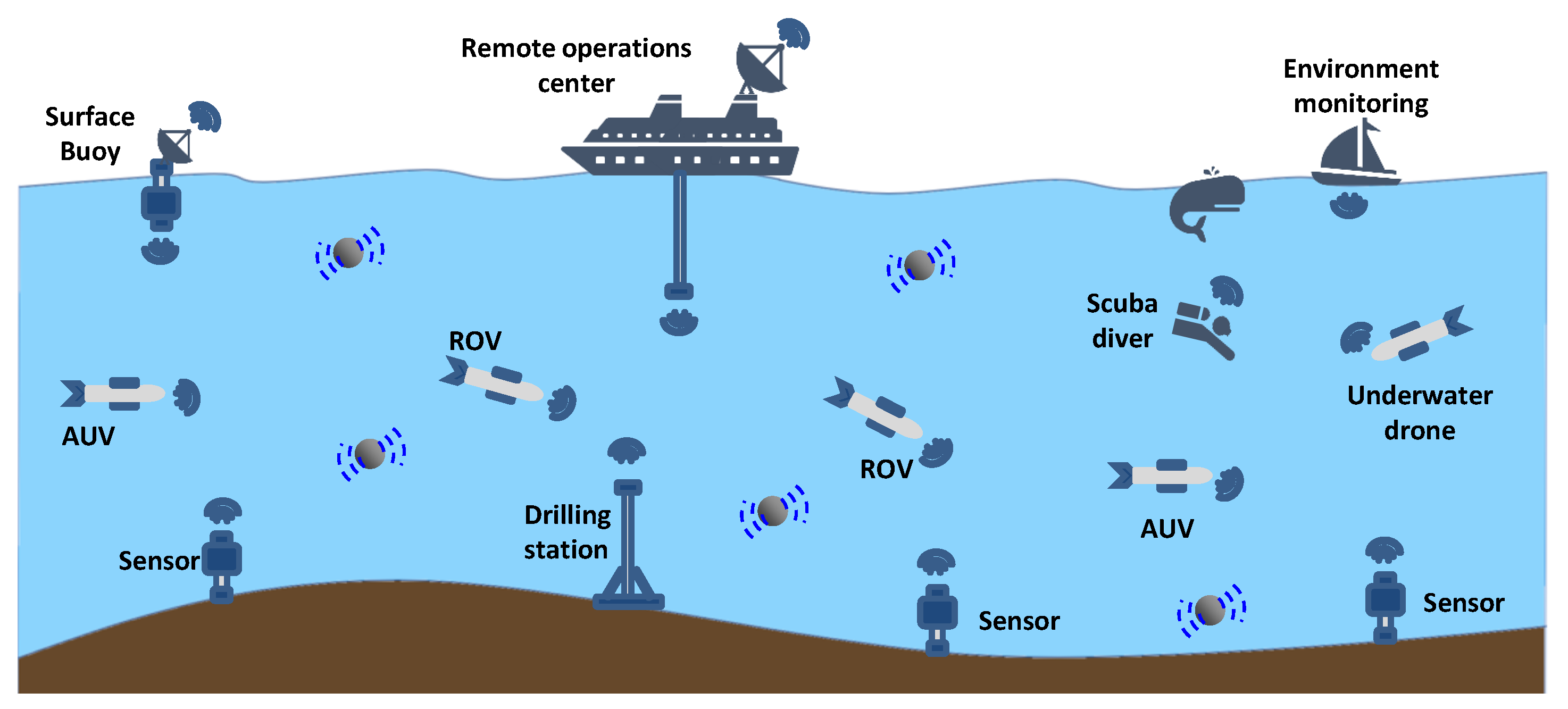
The proposed algorithm for transmission power control is designed to minimize energy consumption in a multi-hop underwater network environment, as depicted in Figure 1, where multiple battery-powered underwater communication devices—sensor nodes, sensor gateways and AUVs—share the same transmission medium and communicate with each other. Instead of relying on a direct transmission from a source to a destination, the algorithm employs relays—the network nodes located inbetween the selected source and destination. Since acoustic communication is known for its high energy consumption, and the energy needed for the acoustic signal needed to reach a destination increases exponentially as the distance increases [7,25,26], a number of relays along a direct path from the source to the destination can significantly improve the overall energy efficiency of the network system. However, every relay would consume its own power to forward the message further, thus increasing the total energy consumption. Therefore, it is crucial to find a theoretical balance between the energy required to send a packet directly towards a destination, and the total energy needed to deliver the same packet over a number of relays.
The proposed protocol relies on the forwarding and the RL-feedback algorithms to adjust to the most energy-efficient path from a source node to a destination node. The protocol selects next-hop relays which are the closest ones to the optimal distance estimated by our algorithm. In another word, a sender—either the original source or a relay—tries to find a next-hop relay located as close as possible to the optimal distance. The sender then sends the packet using the reduced transmission power, just enough to reach the relay, and finally gets a reward back from the relay.
The forwarding algorithm runs on the sender side whenever a packet needs to be delivered to a destination. The algorithm calculates the corresponding optimal distance and then seeks for the best possible next-hop relay using a softmax method, according to a selection weight.
When a next-hop relay is selected and a packet is forwarded, the RL-feedback algorithm kicks in to adjust the corresponding selection weights for the future transmissions. For this purpose, first, a feedback-reward is generated on a receiver side, based on its actual location; second, the reward is propagated back to the sender, updating the selection weight for the chosen relay.
In this section, we will first explain the underwater acoustic propagation model and the optimal distance in Section 3.1. Then in Section 3.2 we will describe the forwarding algorithm in details, followed by the learning algorithm in Section 3.3. Afterwards, we will present an example in Section 3.4 to connect all the dots and show how the proposed protocol works.
3.1. System Model
According to [7], the underwater acoustic attenuation can be modeled as:
where l is the distance between the source and destination and k is the spreading factor ( in underwater environment). is the absorption coefficient determined by the acoustic channel frequency f. According to [25], can be modeled as:
The overall energy consumption, , using n relays can then be estimated by
where n is the number of intermediate relays, L is the direct distance from the source to the destination, f is the central frequency of acoustic signal, k is the spreading factor, is the threshold of receiving signal power, is the transmission delay in seconds and is the power consumption for receiving a signal.
Figure 2 shows the energy consumption from a source to a destination with a distance of L. We change the number of relays from 0, i.e., direct transmission without a relay, to 10 relays. It can be noticed that the longer the distance L between source and destination is, the more transmission power is required to deliver a signal to a destination, which should be strong enough to be recovered (i.e., above a hardware determined receiving threshold). It can also be observed that, when the distance L between a source to a destination is long (i.e., >3 km), the energy consumption is skyrocketing as the number of intermediate relays reaches 0. On the other hand, if L is not very long (i.e., 1.5 km), the introduced relays can actually harm the overall energy efficiency of a path, since: (1) every new introduced relay does not shorten the direct distance sufficient enough to take advantage of the non-linear signal attenuation; (2) the energy consumption of every new relay adds up, hence increasing the total energy consumption.
The proposed algorithm employs relays instead of direct transmissions. As indicated by Figure 2, this scheme can operate efficiently when the communication range of the underwater sensor nodes is over 3 km. In fact, the range of many commercially available underwater acoustic modems [5,27,28] is in excess of 5 km. Therefore, we consider the proposed protocol to be very feasible in practical settings.
So far, from Equation (4), we can easily locate the function’s minimum; now it is possible to estimate the optimal inter-hop distance between relays to achieve maximum possible energy efficiency. For example, for a source-destination pair 3000 m away, the number of optimal helper-relays would be 2 (Figure 2). Therefore, the optimal distance can be estimated as m, where is the optimal distance between relays, is the direct distance between source s and destination d, and is the optimal number of helper-relays for a given direct distance, found as a function minimum of Equation (4).
3.2. Forwarding Algorithm
The forwarding algorithm is executed on the sender- and relay-nodes while forwarding a packet towards a destination. It is described as Algorithm 1 below.
| Algorithm 1 Packet Forwarding Algorithm |
| 1: Assign s to be an address of a sending node |
| 2: Assign Get packet p to send |
| 3: Read destination d of p |
| 4: Read of p |
| 5: Get towards destination |
| 6: Calculate |
| 7: for all possible next-hops j do |
| 8: Update based on Equation (6) |
| 9: if then |
| 10: |
| 11: else |
| 12: |
| 13: Adjust Tx power to reach next hop (Equation (11)) |
| 14: Send p to next hop |
| 15: Set IA expiration timer |
First, the current sender s obtains a packet p to send—either from the MAC-layer’s send-queue (if the sender is the originator of p), or from the PHY-layer (if the sender is a relay, i.e., it has received p from a previous sender).
Second, the sender s reads the destination address d from packet’s header and calculates the current optimal distance . This metric is then recalculated on per-packet basis, i.e., for every new packet to be sent, the optimal distance is recalculated to accommodate possible changes in the network conditions. After calculating , the sender estimates the selection weights for a next-hop relay by comparing and for every possible next-hop j, as expressed by:
where is a direct distance from the source s to next-hop j, is an optimal inter-hop distance from the source s towards destination d.
Third, an actual next-hop relay is selected non-deterministically, using a function which converts the estimated weights to selection probabilities :
Such a probabilistic way of selecting next-hop relays can be beneficial in networks with dynamic topologies such as UWSNs, where the properties of a certain link might significantly vary in time. Small random variation in relay selection emphasizes exploration for every possible action, bringing a balance between the exploration vs. exploitation problem described in the Reinforcement Learning literature [29].
Finally, the actual next-hop node is selected randomly from a list of all possible relays, according to their selection probabilities—i.e., the higher is, the higher chances for j to be selected.
In the case when a node has obtained the packet from the PHY-layer, meaning the node is a relay for a given packet p, the node does an additional check for a hop count expiration. That is, if of p exceeds maximum allowed hop count number, MAX_TTL, the node force-selects the final destination of p to be a next-hop relay.
3.3. RL-Feedback Scheme
The RL-Feedback scheme can be divided into two parts—the receiver part, where a feedback-reward is generated and sent back to the previous sender, and the sender part that waits for the incoming reward to update the selection weights for optimizing future relay selections, hence improving the energy efficiency.
3.3.1. Reward Generation
For the proposed RL-based algorithm, a difference between the optimal and residual distances is chosen as the main argument of the reward function. By residual distance , a difference between the direct distance and a distance from the current relay j towards the final destination d is considered:
Thus, the residual distance describes a relay-node perspective on how energy-efficient the relay is for a given (src, dst) pair. If is greater than , meaning that the relay-node is located farther away along the optimal path, the previous sender should receive a small feedback-reward for the chosen relay. On the other hand, if the values of and are close to each other, the previous sender has been able to select a “good” relay, meaning that a high reward should be sent back to reinforce this relay to be selected in the future. The reward-generation algorithm is proposed as Algorithm 2 below, with the reward calculation function as follows:
Equation (9) emphasizes the fact that the reward is based on current location of the receiver and how far it is from the destination node. Naturally, the closer the receiver’s location to the optimal distance is, the higher the reward would be.
| Algorithm 2 Reward Generation Algorithm |
| 1: Receive packet p from PHY-layer |
| 2: Read from the packet header |
| 3: Get distance from current node to the destination |
| 4: Generate reward based on Equations (8) and (9) |
| 5: Insert into packet header |
| 6: if then |
| 7: Send explicit message back to previous sender |
| 8: else |
| 9: Perform next-hop relay selection based on Algorithm 1 |
| 10: Send packet to next relay, with enough Tx power for the previous sender to overhear it |
3.3.2. Weight Update
On the sender-side, a node uses Implicit Acknowledgements (IA) to extract a reward information. In other words, it expects to overhear a packet transmission on a relay it has previously sent the packet to. In the case when the next-hop relay is the destination itself, the sender expects to receive an explicit reward message back.
Denoting as the learning rate, upon the reception of either an IA or a reward message, the sender updates the selection weight of a given relay in the following manner:
If no IA or reward message is received before the timer expires, which is set right after packet transmission, a default negative reward is assigned to Equation (10). The corresponding algorithm is presented in Algorithm 3.
| Algorithm 3 Weight Update Algorithm |
| 1: Initialize reward |
| 2: if then |
| 3: Assign negative reward: |
| 4: else |
| 5 Assign reward from packet header: |
| 6: Update selection weight using Equation (6) |
3.4. Operation Example
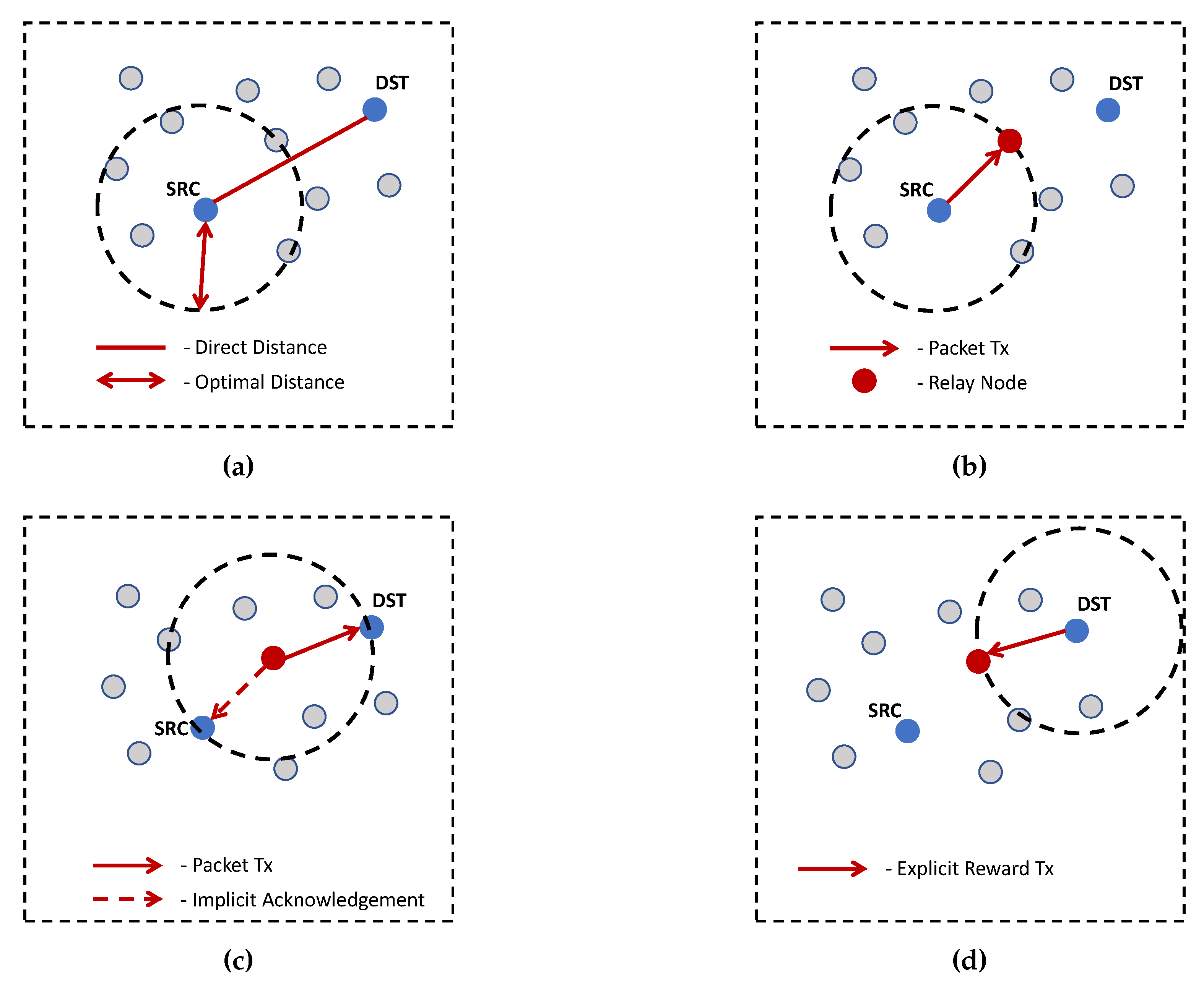
In this section, we present an example to demonstrate the operation of the proposed protocol. Let us consider a fully-connected underwater network of 12 nodes randomly placed within a rectangle area, as depicted in Figure 3. At the beginning of the operation (Figure 3a), a source node (SRC) has a packet to send towards a one-hop destination node (DST). The SRC node then estimates a direct distance to the DST node and calculates the optimal distance , where s is the source node ID, and d is the destination node ID.
Given the optimal distance and the direct distance , the SRC node performs the node-selection operation, according to the Algorithm 1. In this particular example, divides the direct distance into two parts, implying that the optimal number of relays is 1. The number of relays can be bigger or smaller, depending on the two factors: 1, direct distance in a src-dst pair which defines the optimal distance; 2, actual positions of the intermediate nodes, which may or may not be located along the direct path from the source to the destination. As a result, the SRC node finds a relay-node (red circle in the figure), which location “splits” the direct path into two segments, close to the optimal distance. Based on Equation (9), this relay-node would get the highest reward. Therefore, it would get the highest chance to be selected, according to the selection probabilities calculated in Equation (7). Eventually, the SRC node transmits the packet towards the relay-node (Figure 3b).
The relay-node receives packet from the SRC node, reads the optimal distance value from its header and finds a node which is the closest one to the DST node, within the optimal distance. The relay-node selects the DST node for the next transmission, since it is located closer to the optimal distance. Indeed, every other next-hop option would only increase the path distance, bringing it farther away from the optimal metric. Thus, the relay-node selects the DST node and forwards the packet towards it, Figure 3c.
While a packet is propagated towards the DST node, its signal would also be overheard by the previous sender—the SRC node. This becomes possible because of two factors: 1, an omni-directional transmission is assumed; 2, the sender (relay-node) makes sure that the previous sender would get a packet by adjusting its Tx power, given the distance between the relay-node and SRC node. When the SRC node gets a copy of a packet sent from the relay to the DST node, it reads its header, obtains a reward from it, and updates its selection weights for future transmissions. Such “overheard” packets are often called the Implicit Acknowledgments (IA) in the literature and, in this paper, they implement a feedback mechanism, required for the RL-based algorithm of the relay selection. The IA reception is also depicted on Figure 3c.
Finally, the DST node receives packet from the relay-node (Figure 3d). After a successful reception, the DST node sends an explicit reward-message back to a previous sender—the last relay node. Such a reward message is necessary, because the final destination would not forward the packet any further and, thus, the previous sender would not overhear any IA. In other words, an explicit reward-message is only sent by the destination node to a previous node the destination has received a packet from; the implicit acknowledgements carry the rewards to the previous senders in the rest of the cases.
Path Energy Estimation
Assume that every node in the example above is able to transmit a packet at maximum of 60 Watts of power on a 25 kHz central frequency. The direct distance from the source to the destination node is equal to 2000 m. Given this information, now it is possible to estimate the energy spent on transmitting a packet from the SRC to DST node, and compare it with the energy which could have been consumed for a direct transmission, without the helper-relay.
The minimum transmission power required to send a signal from the source directly to the destination can be calculated using the Rayleigh attenuation model:
where is the required transmission power (in Watts), is the received signal threshold for successful decoding (equaled to for this example), l is the distance between the source and destination (2000 m), is the spreading factor ( in underwater environment), and is the absorption coefficient determined by the acoustic channel frequency f (25 kHz), according to Equation (2) (Thorp equation [7]). Thus, the transmission power for direct transmission would be Watts.
Now, for the simplicity, assume that the introduced intermediate relay is located equally far from the SRC and DST nodes, and its distance to both of them is equal to 1100 m. Therefore, given the same inputs as above, the total transmission power required to deliver the same packet to the destination through the relay would be equal to Watts, where is the total Tx power required to send a packet from SRC to DST via the relay and is the Tx power required to send a packet to and from the relay (1-hop transmission).
Thus, the difference in the transmission powers between direct vs. 1-relay transmissions is 7.47 times, which is substantial, especially considering that the underwater acoustic transmission power dwarfs the receiving power. For instance, the relevant reception power for a conventional 60-Watt acoustic modem varies around 0.8 Watts [5].
4. Performance Evaluation
In this section, we compare the proposed LIBRA protocol with two conventional MAC protocols for UWSNs–ALOHA [8] and SFAMA [30], which are described in Section 4.1. Then we introduce three simulation scenarios used in this paper and the performance metrics in Section 4.2. Following that, we present and explain the simulation results in Section 4.3. The comparisons focus on the network throughput, number of collisions and the energy efficiency. In addition, we evaluate the adaptiveness and effectiveness of the learning algorithm. Finally, we summarize the findings from the simulation results and present a discussion in Section 4.4.
As for the toolset used to evaluate the performance of compared protocols, aqua-sim-ng [31], an NS-3 based network simulator for UWSNs, is selected. As an extension to the NS-3 simulator, the aqua-sim-ng simulator leverages all the functionalities of the well-known and powerful NS-3 framework, introducing underwater communication models for the physical, MAC and routing layers. All protocols involved in the simulations are implemented in aqua-sim-ng.
4.1. Compared Protocols
Two conventional MAC protocols for UWSNs have been selected for performance comparisons. The first one is ALOHA [8], which is a classic MAC protocol, based on contention-based channel access mechanism. The second protocol is Slotted Floor-Acquisition Multiple Access (SFAMA) [30], which uses contention-free channel-reservation mechanism to share and access the channel resources.
In the following subsections, generic algorithms of ALOHA and SFAMA will be presented, alongside with their default operational parameters used in the simulations and comparisons.
4.1.1. ALOHA Protocol
ALOHA protocol is based on a simple contention-based channel access algorithm, described in the following steps. First, before sending a packet, the sender checks its network device, attached to the channel. If the network device is busy, i.e., the node is transmitting or receiving something to/from the channel, do a random transmission backoff within the specified time window, defined as a configuration parameter. Second, when the sender returns from the backoff, it checks the network device once again and, if it is free, do send the packet and go to the next one in the queue. Third, if the channel remains busy, keep doing the backoffs until the channel is free or a packet transmission deadline is reached. If the packet transmission deadline is reached, force the packet transmission regardless from the channel state, causing a possible collision, or drop the packet. The packet transmission deadline is a configurable parameter in the implementation.
For the simulation scenarios in this paper, an existing implementation of ALOHA protocol for underwater networks was used, provided by the aqua-sim-ng simulator. The default configuration parameters for the ALOHA implementation used in the experiments is presented in Table 1.
4.1.2. SFAMA Protocol
SFAMA protocol [30] uses a contention-free channel reservation mechanism for scheduling packet transmissions among the nodes sharing the same underwater channel. First, before data transmission, the sender generates and broadcasts an Request to Send (RTS) message across the network, if the channel is free. The nodes receiving the RTS remain silent within a pre-defined slot interval, equalled to the maximum packet latency—the sum of the maximum propagation delay and transmission delay for a packet. Such a slot duration guarantees collision-free transmissions, since every node in a network would be able to overhear and defer the transmissions no later than the maximum packet latency. Second, at the beginning of the next slot, the destination broadcasts a Clear to Send (CTS) message back to sender. As the CTS message propagates over the network, all the other nodes would know the start and the end of the data transmission for a given sender-receiver pair and will remain silent. Third, when the sender get a CTS from receiver, it sends the data packet. Finally, when the receiver successfully gets the data packet, it responses with an ACK back to the sender, informing it about the successful data transmission, so that the sender can process the next packet in its queue.
If two or more nodes are trying to reserve a data transmission at the same time, a collision within the RTS or CTS phase might occur, since the nodes are competing for the shared channel resources. That means a node making a reservation might overhear another incoming RTS or CTS. In such a case, the node would defer its RTS/CTS handshake and keep silent during a randomly selected number of backoff slots. After that, a node tries to reserve a new time-slot for the same data packet transmission.
Besides the main RTS/CTS/data/ACK mechanism described above, SFAMA may use a number of additional features to improve its performance. For instance, SFAMA may send data packets back-to-back in a single RTS/CTS exchange. This is called a packet-train, the size of which can be configured separately. It may also use different priority schemes for particular packets as well as enabling/disabling the final ACK transmission. These parameters are assumed to be configurable as well.
SFAMA protocol has also been implemented in the aqua-sim-ng simulator. Its default configuration parameters which then were used in the simulation experiments are presented in Table 1.
4.2. Simulation Scenarios
To be able to evaluate the performance of the protocols, three simulation scenarios were implemented.
- Adaptiveness Scenario
The adaptiveness scenario was designed to evaluate the performance of the adaptive learning algorithm of the proposed protocol when the distance inbetween the nodes is exactly the optimal distance, so that the protocol would quickly find and converge to the optimal path. We plan to observe how much total energy consumption has been eventually consumed, and how many different path variations have been selected prior to converging to the optimal path.
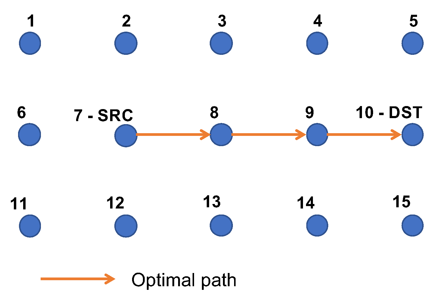
For this purpose, we design a network topology consisting of 15 nodes placed into the corners of 3 × 5 grid, as shown on Figure 4. The optimal distance was set to the length of an edge between the two closest nodes. The source node ID is 7, the destination node is 10. We assume the SRC node transmit packets with a fixed packet rate towards the DST node. Based on this configuration, the most energy-efficient (optimal) path becomes obvious—that is the 7-8-9-10 path.
The task of the protocol was to converge to the optimal path after a number of “trials”—packet transmission events. We will demonstrate how the randomized soft-max selection algorithm of the proposed protocol behaves in such a configuration in Section 4.3. We will be particularly interested in how fast the protocol converges to the optimal path.
For every path selected by the protocol, the path energy consumption was calculated as following:
where is the receiving time of incoming packet; is the receiving power of incoming packet; is the transmission time of packet; is the transmission power of packet; is an energy consumption of the nodes in IDLE state (when no Tx/Rx events occur). In the simulations, and were set to 0.158 Watts [32], whereas was adjusted dynamically by the protocol.
- Energy Scenario
Different from the adaptiveness scenario, in the energy scenario, we focus on the performance in random topologies, in which the node distance is no longer the optimal distance. This is more realistic than the previous scenario. The objective is to test and compare the energy-related properties of the proposed proposal with those of ALOHA and SFAMA in realistic situations.
For this purpose, different network density scenarios were implemented, by increasing the number of nodes within the same 10 × 10 km area, placed randomly. We would like to see how different densities affect the energy efficiency of the protocols. The task of the protocol was to find and use an optimal path, that is, the path with the minimum energy consumption. It will be showed “how far from optimal” the selected path turned out to be. This is expressed in a special metric, called energy efficiency—a ratio between energy consumption of the truly optimal path and the energy consumption of the path(s) actually selected by the protocol.
The network traffic is generated by picking random pairs of source and destination nodes for data transmission. Since we are exploring the optimal possible energy efficiency in this scenario, we would like to reduce the energy waste caused by interference and packet collisions. Therefore, a low packet rate of 0.01 pkts/sec has been chosen specifically to avoid any possible packet interference and collision events, which could have been introduced by the relay-nodes during the packet forwarding. This provided more accurate environment for calculating pure-energy metrics of the protocol, filtering out additional energy overheads due to possible packet retransmissions and random backoffs which could have occurred with higher packet rates.
The following energy metrics will be evaluated for this scenario:
- Total energy consumption : total energy consumed by a network during packet transmissions, in Joules:where —energy consumption for sending a single packet over path i; —number of packets sent over path i;
- Energy per bit : a fraction of the total energy, spent on every successfully received bit of information, in Joules:where is a total number of successfully received packets; —packet size, in Bytes;
- Energy efficiency : a fraction between the most energy-efficient (optimal) solution and the actual of a protocol:where —truly optimal energy consumption, pre-calculated for every given SRC-DST pair.
- Traffic Scenario
The traffic scenario was implemented to provide an evaluation of the maximum network throughput for the protocols being compared. For such scenario, the density of a network was fixed to 1.28 nodes per squared kilometer (which is equivalent to 128 nodes in 10 × 10 km area), while the packet generation rate varied from 0.01 to 0.6 packets per second. For the traffic scenario, every single node in a network was generating packets towards randomly chosen destination, according to the Poisson distribution with rate .
The density of 128 nodes in 10 × 10 km area has been chosen to ensure the connectivity of the network, considering that every node had 3000 m of the maximum transmission range. Given that range and the density, an average number of nodes in 3000 meter radius can be estimated around 36 nodes, providing a good variation in the src-dst pairs as well as creating a lot of possible path-options the proposed protocol can select from. This would pose a challenge to the proposed path-selection algorithm.
The following performance metrics were calculated for the traffic scenario, in addition to the previous ones:
- Total throughput : the total amount of received bits per second, in bps:where is a simulation duration, in seconds;
- End-to-end delay : the time spent for delivering a packet from a source’s application layer to a destination’s application layer, in seconds:where —timestamp when a packet is sent from the application down to the network stack; —timestamp when a packet is received and sent up to the application;
- Collisions per packet : how many collisions are caused by a single data packet transmission, in average:where is a total amount of collisions occurred; is a total number of transmitted data packets;
- Tx events per data packet : how many Tx events were caused by a single data packet, in average:where —total amount of Tx-events occurred in a simulation run;
- Rx events per packet : how many Rx events were generated by a single packet transmission (including service messages):where —total amount of Rx-events occurred in a simulation run; —total amount of transmitted packets, including both data and service messages.
For all scenarios, the maximum transmission range was fixed to 3000 m, with 60 Watts of maximum Tx power. Packet size was fixed to 800 Bytes. Simulation time was set to 1000 s. Additional parameters for both scenarios are presented in Table 2.
4.3. Simulation Results
The simulation results for all scenarios described above were averaged over 1000 iterations for every simulation run. The standard deviation of the simulation results is listed in Table 3.
4.3.1. Adaptiveness Scenario
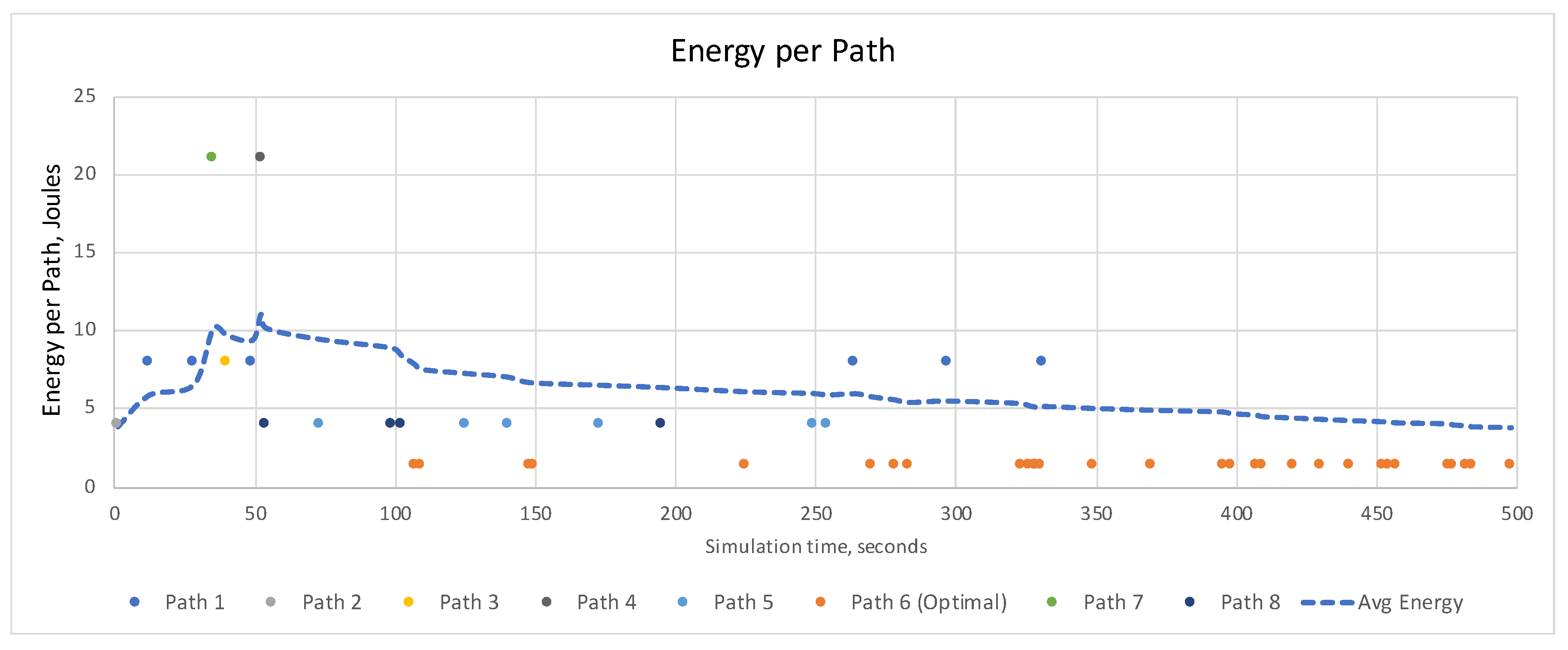
Figure 5 shows how the proposed protocol operates under the simulation scenario visualized in Figure 4. The protocol was able to quickly find the optimal path after 10 packet transmissions (attempts), and saved a substantial amount of energy from the beginning of the operation. As the packet transmission went on, the average path energy consumption was decreasing since the protocol was getting closer to the most energy-efficient path until it finally converged to it after 30 attempts, providing the maximum possible energy-efficiency thereafter.
At the beginning of the operation (when the simulation was initialized and the first packet was generated at the source), the protocol was trying to find the optimal path, until it finally converged to it at the simulation time around 350 s, that is, the protocol started to use only the optimal path (path 6) after 350 s simulation time. In the interval between 0 and 350 s simulation time, the protocol was under a path discovery phase, where the different path variations were tried out from path 1 to path 8, as shown in Figure 5. Every dot in the figure shows a single trial of a particular path, that is, the actual packet transmission from the source to the destination using a specific path. The vertical axis shows the corresponding energy consumed for sending a packet via the selected path.
It also can be noticed, that the first selection of the optimal path (path 6) happened at the 103rd second. However, since the protocol relies on the randomized path selection based on the soft-max algorithm, the protocol was still able to try different path options afterwards. This behavior will be more beneficial in the long run and under dynamic network topologies, since the protocol would still try to discover more options with some probability, even if the current optimal path has already been found.
The dashed line in Figure 5 shows the average energy consumption at a specific time point. Since the protocol converges to the path with the minimum energy consumption over time, the average energy consumption also decreases over time. This is one of the main advantage of the proposed protocol—even if some number of non-optimal paths were selected at the beginning, the protocol is still able to achieve excellent energy efficiency over time and remain flexible to network topology fluctuations at the same time.
Another interesting property of the proposed protocol is how its convergence time, i.e., the time the protocol has spent to converge to some path, depends on the traffic rate from the source. In the given scenario, the source was generating traffic towards destination with 0.01 pkts/s rate. This explains the 350 s convergence time of the protocol, because the protocol did not have enough events (packet transmissions) to converge faster. In other words, if the packet traffic was higher, the protocol would have found the optimal path faster.
4.3.2. Energy Scenario
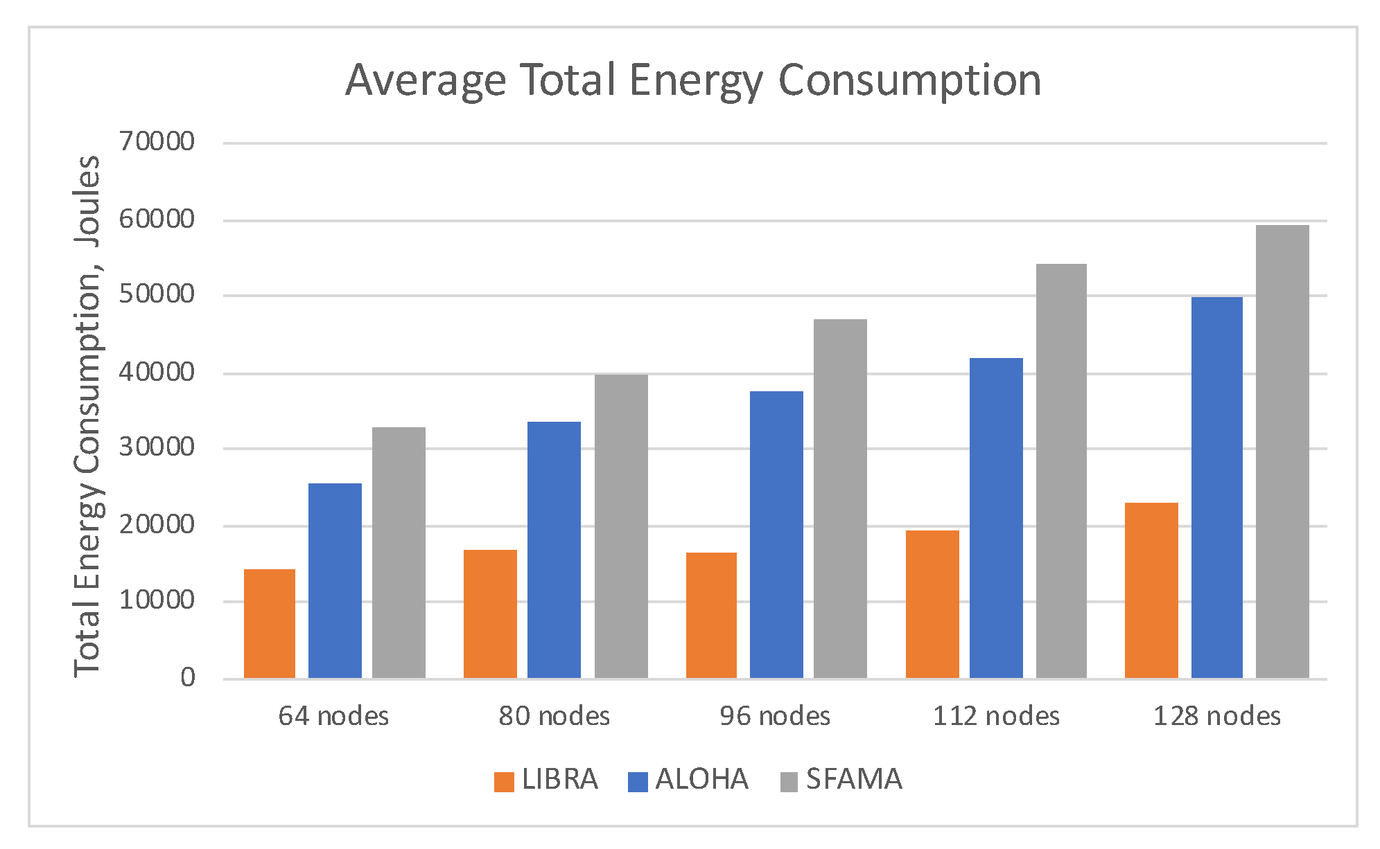
In terms of the energy efficiency for different density conditions, the proposed protocol shows a significant advantage, compared to ALOHA and SFAMA. This can be observed in Figure 6 and Figure 7, which show total energy consumption of a network and the energy per received bit, correspondingly. The figures show that, as the number of nodes in 10 × 10 km area increases, the average energy consumed on the selected path also increases. This behavior is true for SFAMA and ALOHA, while the proposed protocol shows stable energy consumption over different densities. This is explained by different channel access mechanisms used by SFAMA and ALOHA. SFAMA relies on explicit channel reservation, i.e., it sends RTS message across the entire network before packet transmission, which triggers all the nodes in the area to send the replies with CTS messages back. Obviously, as the number of nodes increases, the number of CTS messages needed to be sent also increases, which consumes more energy.
ALOHA does not use any channel reservation. However, every new introduced node in a network still spends some energy on listening to the packets, coming from the source to the destination node. This is true, because the source node transmits a packet in a 3000 m range, according to the simulation parameters. Since the network nodes are placed randomly in 10 × 10 km area, the chance that some nodes would appear somewhere near the src-dst pair is high.
Even though the proposed transmission scheme is similar to ALOHA in sending sending packets out, the introduced transmission control algorithm significantly reduces possible transmission range due to a decreased transmission power. The reduced transmission range means that less nodes would overhear packet transmissions and, therefore, would not spend any energy on the overhearing. This results in much more stable energy consumption across different network densities.
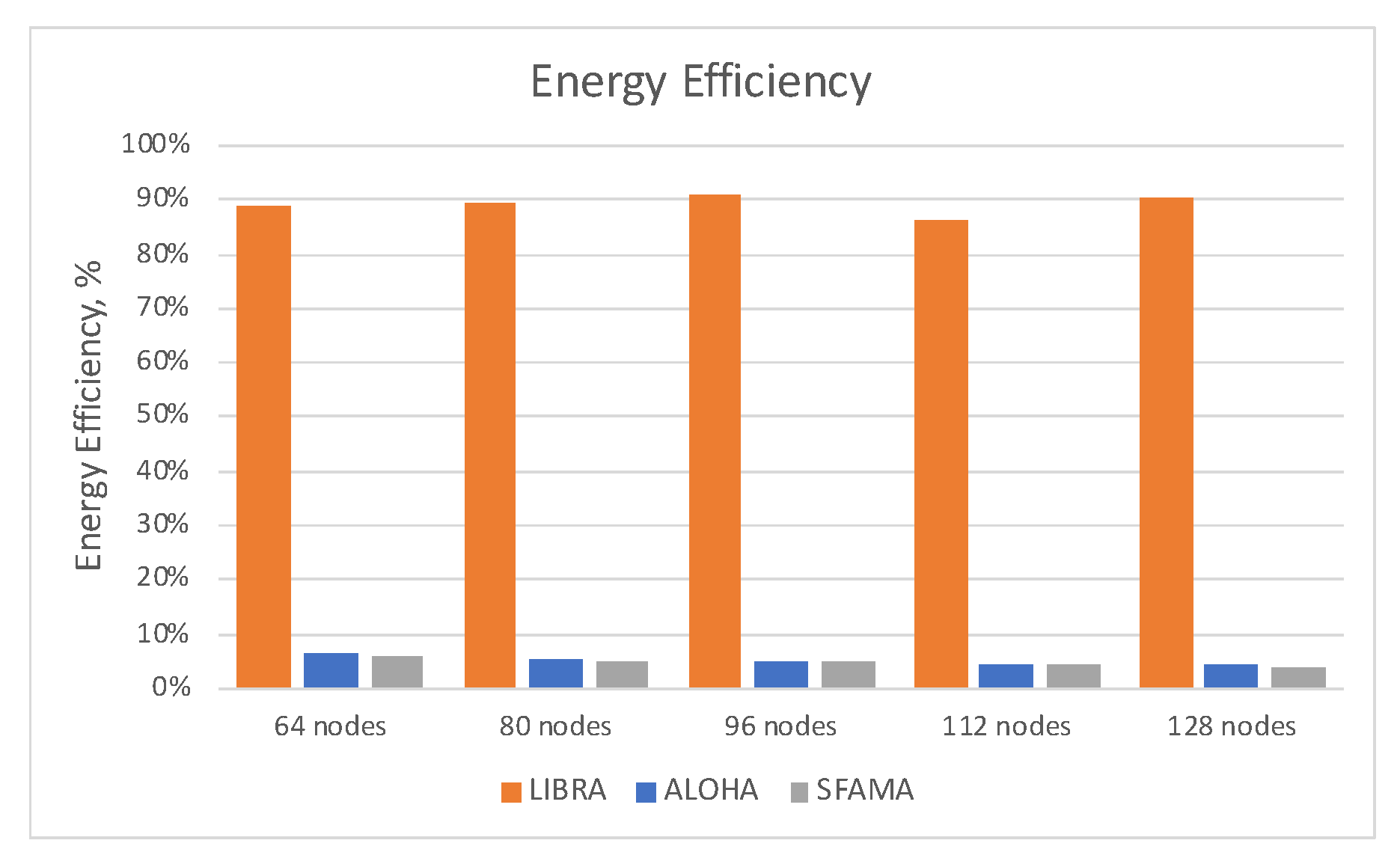
As for the energy-effectiveness of the protocols being tested, the proposed adaptive power control scheme achieves much better performance. Figure 8 shows the energy efficiency—the optimal energy consumption over the actual energy consumption, representing how efficient the protocols are, compared to the optimal solution. The proposed protocol achieves 90% energy-efficiency of the optimal path, outperforming the rest of the protocols. This is largely achieved, again, by the adaptive multi-hop nature of the protocol, which learns from the environment, trying to find the path as close to the optimal as possible. To achieve this, the protocol constantly tries out different paths until it finds a suitable one and starts using it most of the time—the converged path.
4.3.3. Traffic Scenario
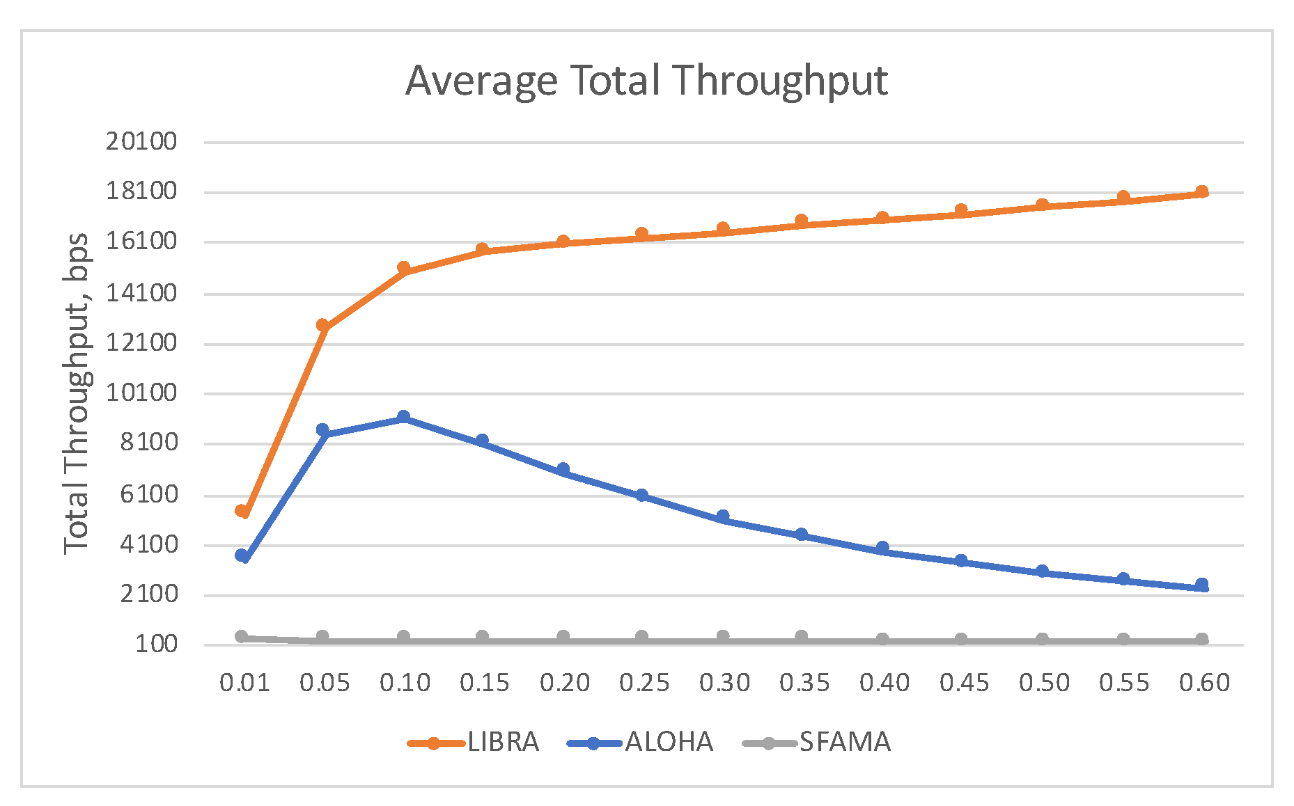
In terms of network throughput, the proposed protocol significantly outperforms both ALOHA and SFAMA, showing up to 80× more throughput, as presented in Figure 9. Such a significant advantage is mainly achieved by two factors: 1, transmission power control, adjusted for a next-hop distance; 2, multi-hop relay operation. The first factor makes sure that the transmission power is small enough so that a packet can only be received by a next-hop relay. This produces less interference among the neighbors and, therefore, creates more opportunities for collision-free simultaneous packet transmissions across the nodes. Considering the traffic-scenario with 128 nodes in 10 × 10 grid area, a number of such possibilities for simultaneous transmissions makes a considerable contribution to much more superior network throughput. The second factor for high network throughput is the usage of multi-hop relays. Even though the original and the main purpose of using multi-hop relays is the energy consumption optimization, the relays also produce a significant amount of duplicate traffic, which is coming from the source nodes. In particular, every relay-node increases the amount of original packets in a network by a factor of N, where N is a number of relays. This increases the chances for the original packets to be received at the destination.
Figure 9 also demonstrates different behavior under variable traffic load. For example, ALOHA shows a throughput degradation after reaching its maximum around 0.10, which corresponds to the theoretical analysis of ALOHA-based protocols [33]. SFAMA, on the other hand, demonstrates stable network throughput which does not degrade over traffic. This is because SFAMA uses deterministic channel reservation procedure to avoid collisions and schedule packet transmissions in time. This behavior also aligns with classical analysis of channel-reservation MAC protocols.
However, the behavior of the proposed protocol is different from both ALOHA and SFAMA. Even though the proposed protocol is similar to pure ALOHA when sending packets down to the channel, its network throughput shows stable increase. This is directly related to the transmission power control algorithm, which reduces the interference range. In addition, the intermediate relays increase the chances for packets to be received at the destinations. This is indicated by Figure 10 and Figure 11, which show how many reception (Rx) events and how many transmission (Tx) events were triggered by a single packet transmission, correspondingly. More Rx events means more nodes could be affected or interfered by the transmission. Figure 10 indicates that SFAMA triggers the highest amount of Rx events, which can be explained by the RTS/CTS messages at maximum transmission range, competing for a single packet transmission. ALOHA also shows higher number of Rx events per packet transmission compared to LIBRA. However, this number quickly degrades as the traffic load increases. This behavior of ALOHA is also logical and can be explained by an increasing amount of Tx backoff-events as the traffic load increases. In contrast, since LIBRA diminishes the collision domain by reducing the Tx power, it shows the lowest amount of Rx events per packet transmission, saving more energy (This is true especially if we assume the power consumption in receiving mode is higher than idle mode.) and allowing more throughput.
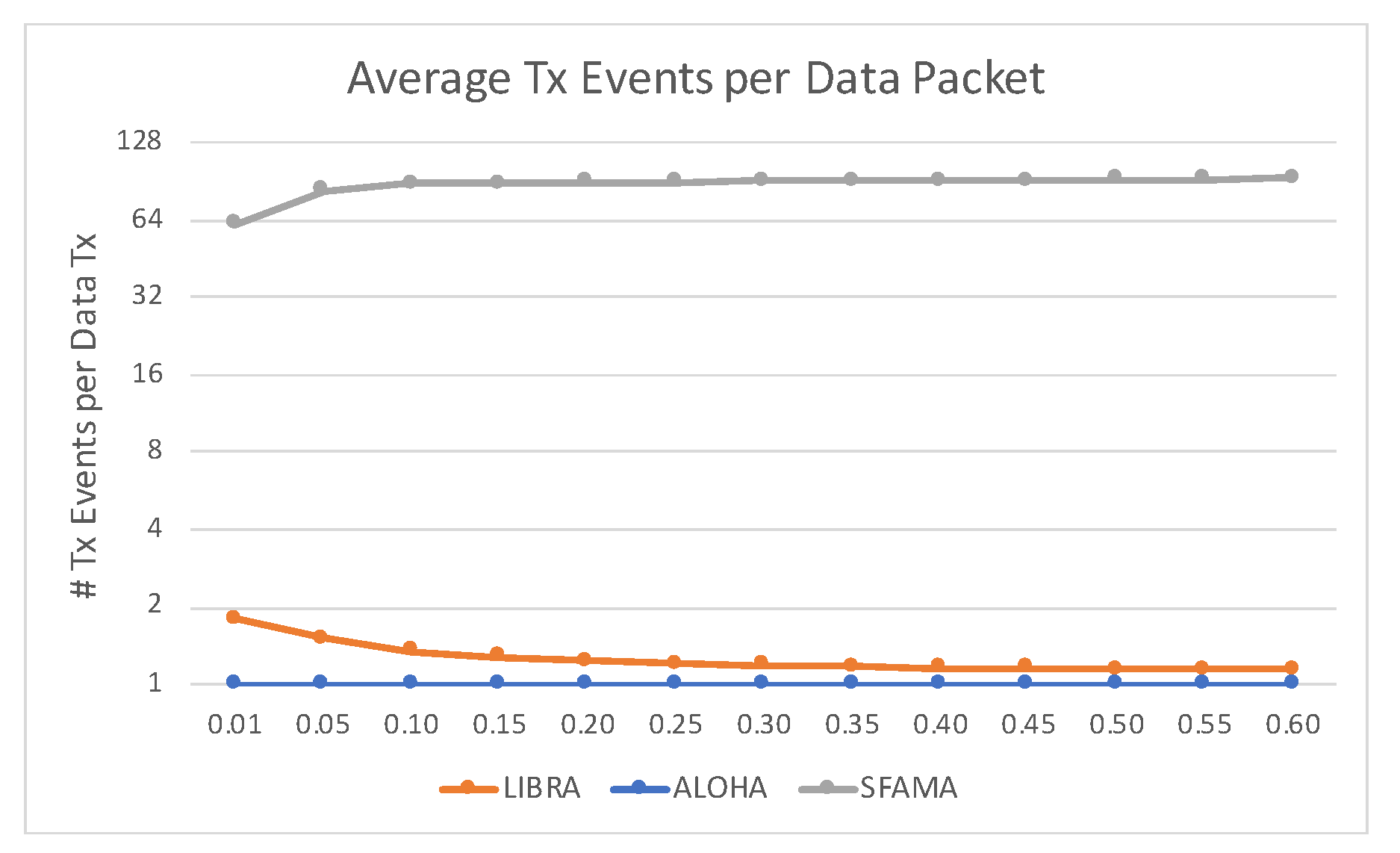
Another interesting behavior of the compared protocols can be observed on Figure 11, which shows how many Tx events were triggered by a single data packet transmission, on average. For instance, ALOHA always shows 1 Tx event per data packet, since it does not rely on any control messages or intermediate relays, it just simply transmits a data packet directly to a destination after a possible backoff. Hence, only a single Tx event is required to send a packet. In contrast, SFAMA uses RTS/CTS message exchanges to reserve a channel. Therefore, it takes some time and efforts until a single data packet can be sent. Since the Traffic Scenario implements a very dense network environment with a high amount of random traffic, it takes a significant number of Tx events until a data packet can be sent in a collision-free manner. A different behavior is shown by LIBRA—even though the protocol does not rely on control messages, it uses the relays to forward a data packet towards a destination. Since every relay forwards the previous message, the average number of Tx events per single data packet is more than one. Figure 11 shows that the average number of Tx events is around 2 for LIBRA (in low traffic), and then it decreases and approaches 1 as the traffic load increases. This behavior is explained by the proposed learning and relay-selection algorithms, which are converging to limit-values as more trials are executed with a higher traffic.
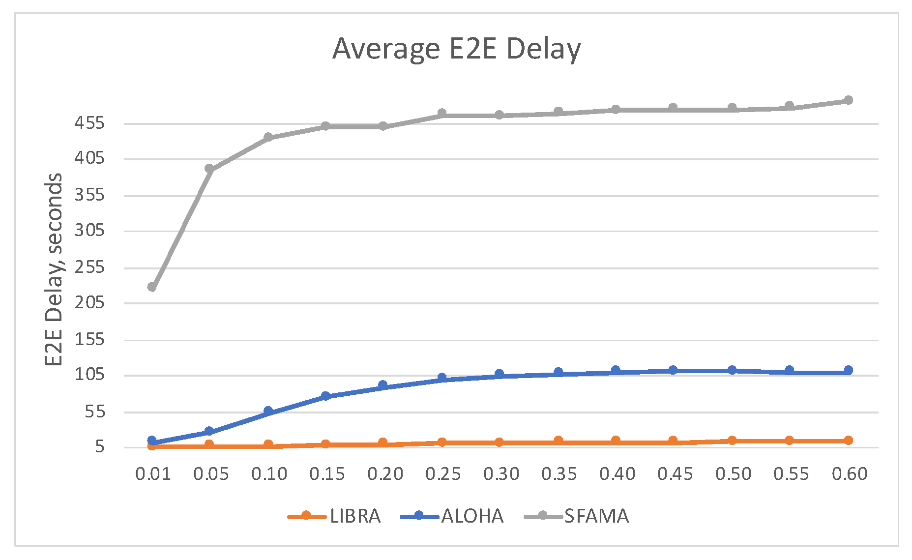
The simulation results also show that LIBRA outperforms SFAMA and ALOHA in terms of the packet end-to-end delay, as shown in Figure 12. SFAMA has the worst performance among the three protocols. This is expected due to its RTS/CTS handshaking process for channel reservation. Because of the long signal propagation delay in the underwater environment, the round trip time can be orders of magnitudes larger than that of terrestrial wireless networks. Hence it is not surprising that SFAMA takes a long time to deliver a data packet. In addition, because the Traffic Scenario simulates a very dense network and SFAMA does not have a power control mechanism, the number of collisions among control messages is high. As previously discussed, SFAMA takes a large amount of transmission attempts before a node can secure the channel for data transmissions (see Figure 11). This further increases the amount of time SFAMA needs to deliver a data packet. ALOHA, on the one hand, does not perform a handshaking based channel reservation. Therefore, it is not sensitive to the long round trip time. That’s why ALOHA works better than SFAMA in terms of end to end delay. On the other hand, ALOHA does not perform any dynamic transmission range control. Therefore, compared to LIBRA, ALOHA’s transmission range is much larger. This creates a larger collision domain and causes a higher number of collisions, meaning ALOHA requires more transmission attempts to successfully deliver a data packet. Further, a bigger transmission range means putting more neighboring nodes into receiving mode or backoff mode, again increasing the end-to-end delay significantly. LIBRA has the best performance because it actively and dynamically adjust the transmission range. With a smaller transmission range, the protocol can reduce the size of the collision domain, hence reducing the number of collisions. This method also make it possible to have multiple concurrent transmissions. All these factors contribute to the good performance of LIBRA in the end-to-end delay comparison with SFAMA and ALOHA.
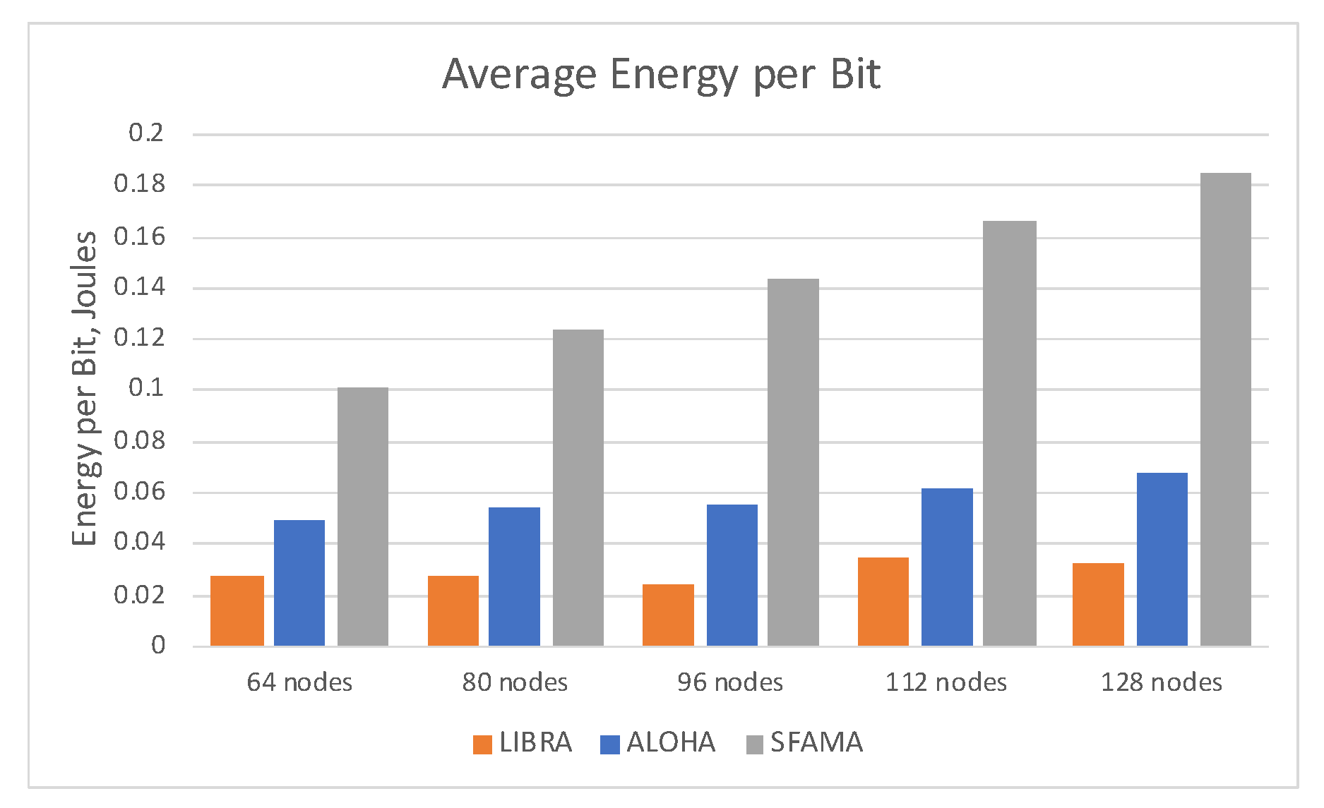
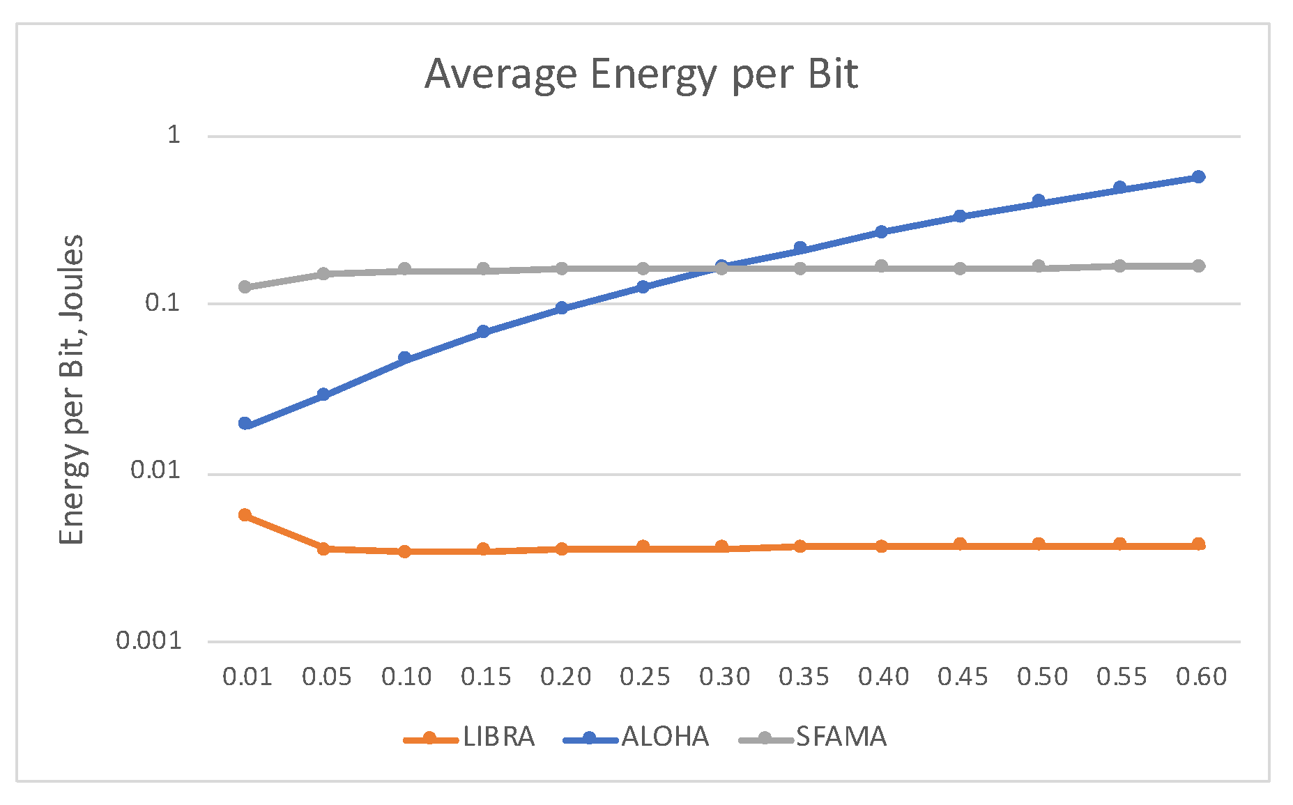
In terms of energy consumption, the proposed protocol consumes much less energy while achieving superior network performance. As shown in Figure 13, the average consumed energy per received bit is the lowest for the proposed protocol and the highest for ALOHA. Here, SFAMA shows the results closer to our protocol, however, the peak difference can be up to 40 times higher for SFAMA.
The advantage in energy consumption can be explained, again, by the transmission power control over multiple relays. As described in the original motivation of this work, every intermediate relay can at most halve the distance between source and destination, thus, saving major part of the energy on transmitting a packet to that relay. This, combined with the improved network throughput, results in much better energy-per-bit performance.
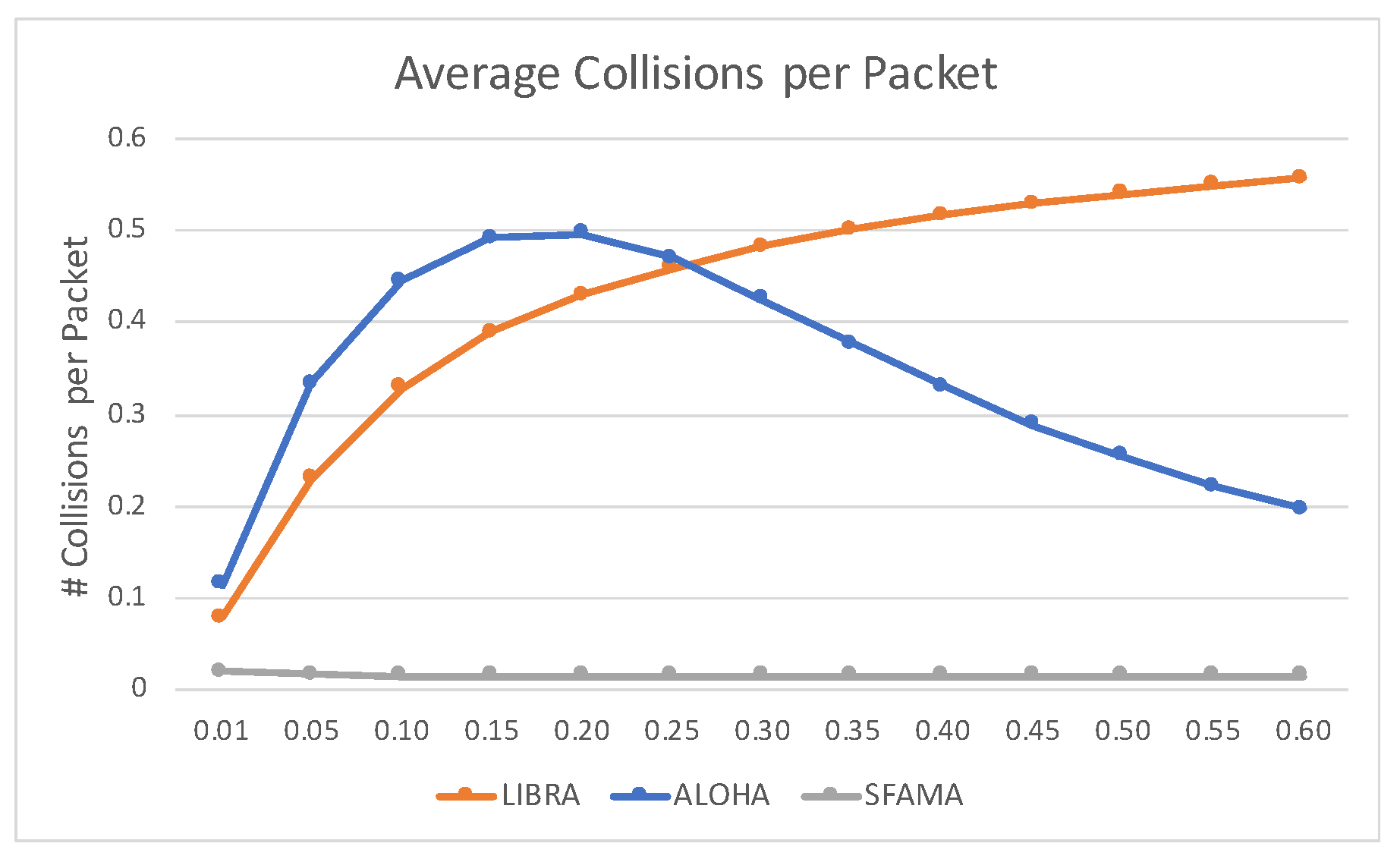
Figure 14 shows average number of collisions per packet. As can be seen from the figure, the behavior of the proposed protocol follows the ALOHA until 0.20 packets/second. After that point, average number of collisions for ALOHA decreases as the proposed protocol continues to send packets to the channel, keeping colliding with the other transmissions. Such behavior can be explained by ALOHA backoff-mechanism, which starts to defer the packet transmissions due to high packet traffic coming from the neighboring nodes. This is not the case for the proposed protocol, since it relies on the power control. This significantly reduces the range of a packet reception that, in its turn, does not trigger the ALOHA-based backoff mechanism, since less packets will be overheard. In other words, ALOHA tends to defer packet transmission as the traffic grows, since it senses more transmissions within the fixed transmission range. In contrast, the proposed protocol uses power control to reduce actual transmission range, encouraging more packet transmissions from the other nodes outside that range. Moreover, the intermediate relays contribute to the collision probability as well, since they increase the original packet traffic, as mentioned earlier. SFAMA performs much differently from ALOHA and LIBRA, since it relies on the channel reservation procedure, which is designed to eliminate data packet collisions. This explains the low metric for SFAMA, as it only considers data packets and excludes services messages, which are still a subject to collisions, since the RTS/CTS channel reservation happens in a contention-based manner, as mentioned in Section 4.1.2.
4.4. Discussions
From the simulation results, we can conclude that the proposed protocol performs well on the MAC layer, compared to the other well-established MAC protocols for UWSNs, i.e., ALOHA and SFAMA. A significant advantage is demonstrated in simulations with regard to the network energy consumption and energy per bit, as well as the total network throughput.
Such an advantage can be explained by the proposed adaptive transmission range control scheme, combined with a contention-based (ALOHA-based) channel access. The first part achieves substantial energy savings by reducing the initial transmission power that, in its turn, opens up the possibilities for collision-free and simultaneous packet transmissions. The second part—ALOHA-based channel access—efficiently utilizes such collision-free transmission possibilities, resulting in the increased network throughput.
The introduced intermediate relays, used by the protocol to further decrease energy consumption, have both positive and negative effects on the network performance. The positive effect can be expressed in the high energy-efficiency, as showed in Figure 8, reaching 90% correlation with the actual most energy-efficient path—the path with the lowest energy consumption. Without the help of relay-nodes, it would not be possible to achieve such low energy consumption, since the intermediate nodes are often the part of the optimal energy path from the source to the destination, in the simulation conditions provided.
However, the use of relays also produces a negative effect. This effect is expressed in much higher packet collision probability for the proposed protocol, introduced by the relays as they forward packets from one node to another. Every such packet forwarding event increases the amount of initial packet traffic in a network and, therefore, quickly saturates local channel capacity. This, combined with non-reliable ALOHA-based channel access, results in high packet collision probability.
Even though we observe high collision probability for the proposed power control scheme, this disadvantage can be justified by the following points. First, according to Figure 14, the collision probability for the proposed protocol is lower than ALOHA in the [0.01–0.25] packet generation rates. Second, as the traffic rate goes higher, ALOHA starts performing more backoffs due to a much larger collision domain than in the proposed protocol, which reduces its collision domain using the adaptive transmission power control. More ALOHA backoffs result in lower collision probability which we see in the figure, but it also results in a network throughput degradation, as confirmed by Figure 9, since less packets are being sent per second due to the increased transmission backoffs. Further, the increased collision probability for the proposed protocol actually means that the protocol is able to push much more traffic through the network, resulting in a significant network throughput gain. This is particularly important, considering that the protocol is also far more energy-efficient at the same time.
In contrast, SFAMA uses channel reservation techniques which avoid collisions but it also results in poor network performance, hardly comparable to those from either ALOHA or LIBRA. However, its solid advantage is the overall stability (i.e., no randomness). SFAMA is the only protocol which achieved near-zero data collision probability regardless of the traffic and show smaller but very stable network throughput. This might be important for some types of UWSNs applications, which would trade throughput performance over network stability. This is an attractive feature of SFAMA, which sheds a light on a possible combination of the proposed transmission power control and SFAMA in the future research. In particular, it would be interesting to investigate how SFAMA (or any other MAC-protocol with a channel reservation mechanism) would be performing, combined with multi-hop adaptive power control algorithm.
Another important conclusion can be drawn from the adaptiveness scenario. As it is shown in Figure 5, the proposed protocol tries out different path options at the beginning of its operation and finally converges to energy-efficient path. Such behavior may be beneficial in the underwater networks with mobile topologies, where the nodes move and, thus, optimal paths also change over time. Furthermore, given that the protocol converges to the energy efficient path after some time, the average energy consumption in a network would also decrease over time and will be reaching optimal values.
5. Conclusions
This paper presents the design, implementation and performance evaluation of LIBRA, a reinforcement learning assisted energy efficient MAC protocol for UWSNs. LIBRA tries to address two issues in a densely deployed UWSN, i.e., packet collisions and power consumption. We design a transmission power control scheme to reduce the collision domain, as well as minimizing system energy consumption. With a reduced collision domain, the protocol allows more network nodes to share the acoustic channel and enables concurrent transmissions within the maximum transmission range. By reducing the transmission power and using intermediate relays, we manage to achieve significant energy savings due to non-linear signal attenuation. Moreover, we design a reinforcement learning based algorithm to select the best relay to further optimize the energy efficiency. Last but not the least, we develop a ALOHA-like transmission scheme with implicit acknowledgements among relays to reduce the end-to-end delay. Simulation results show that LIBRA can achieve good network throughput and low end-to-end delay while significantly reducing the network energy consumption.
As for the future work, we are interested in studying how node mobility would affect the protocol performance. Specifically, we would like to investigate the effectiveness of various learning algorithms on different mobility patterns. In addition, we would like to investigate how other MAC protocols would perform if combined with the multi-hop adaptive power control algorithm. Moreover, in this paper we assume all network nodes have the same communication and computation capability. As a next step, we would like to study how to handle a heterogeneous network which is common in many IoUT applications. Further, we plan to implement the protocol’s prototype in real systems and evaluate the performance in practical and real-world settings.
Author Contributions
Conceptualization, D.D. and Z.P.; methodology, D.D. and Z.P.; software, D.D.; validation, D.D., Z.P., Y.L. and L.P.; formal analysis, D.D. and Z.P.; investigation, D.D. and Z.P.; resources, Z.P.; data curation, D.D. and Z.P.; writing–original draft preparation, D.D. and Z.P.; writing–review and editing, D.D., Z.P., Y.L. and L.P.; visualization, D.D. and Z.P.; supervision, Z.P.; project administration, Z.P.; funding acquisition, Z.P.; All authors have read and agreed to the published version of the manuscript.
Funding
This research was funded by PSC-CUNY Research Award, grant number 61796-0049.
Conflicts of Interest
The authors declare no conflict of interest.
References
- Tabary, Z. The Final Frontier: Who Owns the Oceans and Their Hidden Treasures? Reuters, 3 December 2018. [Google Scholar]
- Doughton, S. Ocean’s Deepest Spot a Noisy Place, Oregon Scientists Find. The Seattle Times, 4 March 2016. [Google Scholar]
- Domingo, M.C. An Overview of the Internet of Underwater Things. Elsevier J. Netw. Comput. Appl. 2012, 35, 1879–1890. [Google Scholar] [CrossRef]
- Zhu, Y.; Jiang, Z.; Peng, Z.; Zuba, M.; Cui, J.H.; Chen, H. Toward Practical MAC Design for Underwater Acoustic Networks. In Proceedings of the IEEE INFOCOM, Turin, Italy, 14–19 April 2013; pp. 683–691. [Google Scholar]
- WHOI. Micro-Modem Specifications. Available online: https://acomms.whoi.edu/micro-modem (accessed on 12 September 2020).
- Murata. TR1000—Datasheet. 2010. Available online: https://www.alldatasheet.com/datasheet-pdf/pdf/106155/RFM/TR1000.html (accessed on 12 September 2020).
- Stojanovic, M. On the Relationship Between Capacity and Distance in an Underwater Acoustic Communication Channel. In Proceedings of the First ACM International Workshop on UnderWater Networks (WUWNet), Los Angeles, CA, USA, 25 September 2006; pp. 41–47. [Google Scholar]
- Chirdchoo, N.; Soh, W.S.; Chua, K.C. Aloha-Based MAC Protocols with Collision Avoidance for Underwater Acoustic Networks. In Proceedings of the IEEE INFOCOM, Anchorage, AK, USA, 6–12 May 2007. [Google Scholar]
- Syed, A.; Ye, W.; Krishnamachari, B.; Heidemann, J. Understanding Spatio-Temporal Uncertainty in Medium Access with ALOHA Protocols. In Proceedings of the WUWNet, Montreal, QC, Canada, 14 September 2007; pp. 41–48. [Google Scholar]
- Filipe, L.; Vieira, M.; Kong, J.; Lee, U.; Gerla, M. Analysis of Aloha Protocols for Underwater Acoustic Sensor Networks. In Proceedings of the WUWNet, Los Angeles, CA, USA, 25 September 2006. [Google Scholar]
- Rodoplu, V.; Meng, T. Minimum Energy Mobile Wireless Networks. IEEE J. Sel. Areas Commun. 1999, 17, 1333–1344. [Google Scholar] [CrossRef] [Green Version]
- Wang, J.; Shen, J.; Shi, W.; Qiao, G.; Wu, S.; Wang, X. A Novel Energy-Efficient Contention-Based MAC Protocol Used for OA-UWSN. Sensors 2019, 19, 183. [Google Scholar] [CrossRef] [PubMed] [Green Version]
- Radha, S.; Bala, G.J.; Stephy, V.; Princy, D.M.; Divya, J.; Sherene, J.R.P. Power Optimization in MAC Protocols for WSN. In Proceedings of the 2nd International Conference on Signal Processing and Communication (ICSPC), Coimbatore, India, 29–30 March 2019. [Google Scholar]
- Doukkali, H.; Nuaymi, L.; Houcke, S. Power and Distance Based MAC Algorithms for Underwater Acoustic Networks. In Proceedings of the OCEANS, Boston, MA, USA, 18–21 September 2006. [Google Scholar]
- Monks, J.P.; Bharghavan, V.; Hwu, W.-M.W. A Power Controlled Multiple Access Protocol for Wireless Packet Networks. In Proceedings of the IEEE INFOCOM, Anchorage, AK, USA, 22–26 April 2001; pp. 219–228. [Google Scholar]
- Ammar, M.; Ibrahimi, K.; Jouhari, M.; Ben-Othman, J. MAC Protocol-Based Depth Adjustment and Splitting Mechanism for UnderWater Sensor Network (UWSN). In Proceedings of the IEEE Global Communications Conference (GLOBECOM), Abu Dhabi, UAE, 9–13 December 2018. [Google Scholar]
- Gomez, J.; Campbell, A.T.; Naghshineh, M.; Bisdikian, C. PARO: Supporting Dynamic Power Controlled Routing in Wireless Ad Hoc Networks. Wirel. Netw. 2003, 9, 443–460. [Google Scholar] [CrossRef]
- Spyropoulos, A.; Raghavendra, C.S. Energy Efficient Communications in Ad Hoc Networks Using Directional Antennas. In Proceedings of the IEEE INFOCOM, New York, NY, USA, 23–27 June 2002; pp. 220–228. [Google Scholar]
- Kwon, T.J.; Gerla, M. Clustering with Power Control. In Proceedings of the IEEE MILCOM, Atlantic City, NJ, USA, 31 October–3 November 1999. [Google Scholar]
- Muqattash, A.; Krunz, M. Power Controlled Dual Channel (PCDC) Medium Access Protocol for Wireless Ad Hoc Networks. In Proceedings of the IEEE INFOCOM, San Francisco, CA, USA, 30 March–3 April 2003. [Google Scholar]
- Sozer, E.M.; Stojanovic, M.; Proakis, J.G. Underwater Acoustic Networks. IEEE J. Ocean. Eng. 2000, 25, 72–83. [Google Scholar] [CrossRef]
- Wei, X.; Zhao, L.; Li, X.; Zou, C. A Distributed Power Control Based MAC Protocol for Underwater Acoustic Sensor Networks. In Proceedings of the 4th IEEE International Conference on Circuits and Systems for Communications, Shanghai, China, 26–28 May 2008. [Google Scholar]
- Qian, L.; Zhang, S.; Liu, M.; Zhang, Q. A MACA-based Power Control MAC Protocol for Underwater Wireless Sensor Networks. In Proceedings of the IEEE/OES China Ocean Acoustics (COA), Harbin, China, 9–11 January 2016. [Google Scholar]
- Chen, Y.D.; Lien, C.Y.; Fang, Y.S.; Shih, K.P. TLPC: A Two-level Power Control MAC Protocol for Collision Avoidance in Underwater Acoustic Networks. In Proceedings of the MTS/IEEE OCEANS, Bergen, Norway, 10–14 June 2013. [Google Scholar]
- Brekhovskikh, L.M.; Lysanov, Y. Fundamentals of Ocean Acoustics; Springer: New York, NY, USA, 1982. [Google Scholar]
- Stojanovic, M.; Preisig, J. Underwater Acoustic Communication Channels: Propagation Models and Statistical Characterization. IEEE Commun. Mag. 2009, 47, 84–89. [Google Scholar] [CrossRef]
- Teledyne Benthos. Acoustic Telemetry Modems: User’s Manual; Teledyne Benthos: North Falmouth, MA, USA, 2006. [Google Scholar]
- EvoLogics GmbH. EvoLogics Underwater Acoustic Modems. Available online: https://evologics.de/acoustic-modems (accessed on 12 September 2020).
- Sutton, R.S.; Barto, A.G. Reinforcement Learning an Introduction; MIT Press: Cambridge, MA, USA, 1998. [Google Scholar]
- Molins, M.; Stojanovic, M. Slotted FAMA: A MAC Protocol for Underwater Acoustic Networks. In Proceedings of the IEEE OCEANS, Singapore, 16–19 May 2006; pp. 1–7. [Google Scholar]
- Peng, Z.; Dugaev, D. The Aqua-Sim NG Official Webpage. Available online: http://hudson.ccny.cuny.edu/mediawiki/index.php/Aqua-Sim_NG (accessed on 12 September 2020).
- NS-3. UAN Framework. Available online: https://www.nsnam.org/docs/release/3.12/models/html/uan.html (accessed on 12 September 2020).
- Kurose, J.; Ross, K. Computer Networking: A Top-Down Approach, 7th ed.; Pearson: London, UK, 2016. [Google Scholar]
Figure 1.
An underwater wireless sensor network.

Figure 2.
Energy consumption over intermediate hops with different distances L.

Figure 3.
Example of the protocol’s operation.

Figure 4.
Network configuration for the adaptivity scenario.

Figure 5.
Energy per packet on every selected path in Adaptiveness Scenario, Joules.

Figure 6.
Average total energy consumption, Joules.

Figure 7.
Average energy per bit, Joules.

Figure 8.
Energy efficiency.

Figure 9.
Total network throughput in traffic scenario, in bps.

Figure 10.
Average number of Rx events per packet transmission.

Figure 11.
Average number of Tx events per data packet.

Figure 12.
Average end-to-end delay, in seconds.

Figure 13.
Energy per bit in traffic scenario, in Joules.

Figure 14.
Average number of collisions per packet.


Table 1.
ALOHA and SFAMA parameters.
| Parameter Name | Value | Description |
|---|---|---|
| ALOHA: | ||
| Min. backoff | 0 s | Minimum backoff time |
| Max. backoff | 1.5 s | Maximum backoff time |
| ACK On | False | Send ACK from receiver or not; False—do not send ACK |
| SFAMA: | ||
| Max. backoff slots | 100 | Maximum number of backoff slots |
| Max. burst | 1 | Maximum number of packets in the train |
| ACK On | True | Send ACK from receiver or not; True—send ACK |
Table 2.
Simulation parameters.
| Energy Scenario | Traffic Scenario | |
|---|---|---|
| Number of nodes | 64–128 | 128 |
| Density | 0.64–1.28 | 1.28 |
| Area | 10 × 10 km | 10 × 10 km |
| Number of src-dst pairs | 1 | 128 |
| Packet rate, pkts/sec | 0.01 | 0.01–0.6 |
| Packet size, Bytes | 800 | 800 |
| Max. Tx Range, meters | 3000 | 3000 |
| Max. Tx Power, Watts | 60 | 60 |
| Channel speed, bps | 10,000 | 10,000 |
Table 3.
Standard deviations as percentage from average, [0.01–0.60] packets/sec, 128 nodes.
| LIBRA | ALOHA | SFAMA | |
|---|---|---|---|
| Total Throughput | 2.57–5.33% | 4.57–15.04% | 20.94–24.48% |
| Energy per Bit | 3.27–5.90% | 4.63–16.16% | 21.93–23.91% |
| Collisions per Packet | 0.97–4.86% | 2.05–7.12% | 37.53–43.49% |
| Rx Events per Tx | 1.00–2.46% | 1.23–6.96% | 8.63–12.02% |
| Tx Events per Data Packet | 0.29–0.67% | 0.47–2.61% | 14.83–17.08% |
| End-to-end Delay | 2.39–2.69% | 8.76–27.36% | 13.31–16.18% |
Publisher’s Note: MDPI stays neutral with regard to jurisdictional claims in published maps and institutional affiliations. |
© 2020 by the authors. Licensee MDPI, Basel, Switzerland. This article is an open access article distributed under the terms and conditions of the Creative Commons Attribution (CC BY) license (http://creativecommons.org/licenses/by/4.0/).
Share and Cite
MDPI and ACS Style
Dugaev, D.; Peng, Z.; Luo, Y.; Pu, L. Reinforcement-Learning Based Dynamic Transmission Range Adjustment in Medium Access Control for Underwater Wireless Sensor Networks. Electronics 2020, 9, 1727. https://doi.org/10.3390/electronics9101727
AMA Style
Dugaev D, Peng Z, Luo Y, Pu L. Reinforcement-Learning Based Dynamic Transmission Range Adjustment in Medium Access Control for Underwater Wireless Sensor Networks. Electronics. 2020; 9(10):1727. https://doi.org/10.3390/electronics9101727
Chicago/Turabian StyleDugaev, Dmitrii, Zheng Peng, Yu Luo, and Lina Pu. 2020. "Reinforcement-Learning Based Dynamic Transmission Range Adjustment in Medium Access Control for Underwater Wireless Sensor Networks" Electronics 9, no. 10: 1727. https://doi.org/10.3390/electronics9101727
Note that from the first issue of 2016, this journal uses article numbers instead of page numbers. See further details here.