Hybrid Energy Network Management: Simulation and Optimisation of Large Scale PV Coupled with Hydrogen Generation

Abstract

The power production of electrical Renewable Energy Sources (RES), mainly PV and wind energy, is affected by their primary source of energy: solar radiation value or wind strength. Electrical networks with a large share of these sources must manage temporal imbalances of supply and demand. Hybrid Energy Networks (HEN) can mitigate the effects of this unbalancing by providing a connection between the electricity grid and and other energy vectors such as heat, gas or hydrogen. These couplings can activate synergies among networks that, all together, increase the share of renewable sources helping a decarbonisation of the energy sector. As the energy system becomes more and more complex, the need for simulation and optimisation tools increases. Mathematical optimisation can be used to look for a management strategy maximising a specific target, for instance economical, i.e. the minimum management cost, or environmental as the best exploitation or RES. The present work presents a Mixed Integer Linear Programming (MILP) optimisation procedure that looks for the minimum running cost of a system made up by a large-scale PV plant where hydrogen production, storage and conversion to electricity is present. In addition, a connection to a natural gas grid where hydrogen can be sold is considered. Different running strategies are studied and analysed as functions of electricity prices and other forms of electrical energy exploitation.

1. Introduction

A power plant is a system that converts one primary source of energy to another form: for instance, in a gas-fired power station, methane is converted to electricity. In a different way, Hybrid Energy Networks (HEN) are characterised by the possibility of creating different power conversion paths. For instance, in a cogeneration plant, natural gas can be converted into heat and electricity at the same time. This feature allows a greater exploitation of the primary fuel with respect to a separate production of heat and electricity. On one hand, this plant is more efficient, while, on the other hand, its management is more complex as its power production must meet dynamically different external parameters such as heating demand or price of electricity sold to the grid.

Another difference that makes the management of HEN more elaborate is the possibility of using energy storage components. Storage can be more economical and efficient when adopted in one energy vector than in another: for instance a thermal energy storage can be less flexible but cheaper than the storage of electrical energy in an electrochemical battery storage.

The research interest toward these kinds of systems is high, as is testified by several strategic documents, such as the recent communication from European Commission on the role of hydrogen for a carbon neutral Europe [1] and by several research projects. The International Energy Agency is carrying out a project aimed at promoting the opportunities for district heating and cooling (DHC) networks by means of an integrated approach, creating a hybrid energy infrastructure between electric grids, gas grids and other energy vectors through various coupling points (CHP, power-to-heat/gas, etc.) [2]. It is in fact well understood that integration of different energy carriers is one of the most promising and effective way to achieve a move toward a decarbonised society [3,4,5,6].

Despite the opportunities that the integration of different forms of energy offers, it must be remarked that this process has to merge different requirements and specific characteristics of each of the carrier involved. In this respect, simulation tools that could incorporate the most important features of all the concurrent phenomena are needed. As a detailed analysis of this multiphysics system can become very convoluted, a suitable level of approximation must be found: on the one hand, the model must be able to catch the technical constraints of all forms of energy involved, while, on the other hand, it should be used efficiently in an optimisation loop to find out the best integration strategy. This trade-off between accuracy and computational cost has been found in recent years to be the hourly time resolution that is able to implement operational constraints, such as energy balance and interactions with market prices and load variations [5].

This work addresses the problem of HENs simulation, tackling the aspect of hydrogen production in the direction of power-to-gas process where electrical energy, obtained by intermittent renewable sources, can be stored, by electrochemical conversion, in a gaseous fuel such as hydrogen. As it is produced by exploiting renewable energy sources, this gas is usually called green hydrogen and can be either pumped in an existing network, such as the natural gas one, or converted locally, producing electricity when the electrical grid is in need. The study and analysis of the process can be approached at different levels, for instance at the national level taking into account both electric and gas constraints [7] or at the local level optimising the share of hydrogen produced by the plant [8]; the second approach is followed in the present work.

Once the system model is defined, several methodologies can be adopted for its optimisation. As, in general, the problem formulation is nonlinear, its optimisation can be tackled by heuristic procedures, such as evolutionary algorithms [9]. Unfortunately, the computational cost of these techniques is usually high and thus an alternative approach resorts to the approximation of the model by linear and/or piece-wise linear equations. In the first case, the use of linear programming techniques is allowed while in the second case the mixed integer linear programming technique is needed. The feasibility of this approach has been already published in the case of complex energy systems [10,11,12,13], which, under the hypotheses of the model, guarantees that the global optimal point is found.

It must also be remarked that optimisation process has to deal with different objectives. As a first issue, the economical return of HEN must be assessed, but it is also true that the impact of these new infrastructures is not negligible. For instance, in the case of large PV plants, the increase of soil usage for energy production should take into account the temporary loss of agricultural land. At the same time, the production of hydrogen needs the electrolysis of water and the use of this natural resource is obviously impacting on the environment. A real multi-criteria optimisation should thus be used as it is already done on some more consolidated plants (see, e.g., [11]). At this stage of HEN development, the availability of an operational optimisation tool enables the quantification of economic return of investment and thus it can be used to assess the viability of scenarios where different environmental politics can be put at stake and compared.

Following the previous considerations, this paper presents a methodological approach for the assessment of a HEN based on the production of electricity by PV with a local storage of energy in the form of hydrogen or by means of electrochemical batteries. The problem is formulated in mathematical terms, highlighting its peculiarities and its implementation in a modular procedure. To assess the computational performance of the implementation, some operational optimisations on a test case study, whose data are derived from literature, are performed. These results show the potential advantages of the approach which can be used to assess different scenarios.

2. Description of the Hybrid Energy System

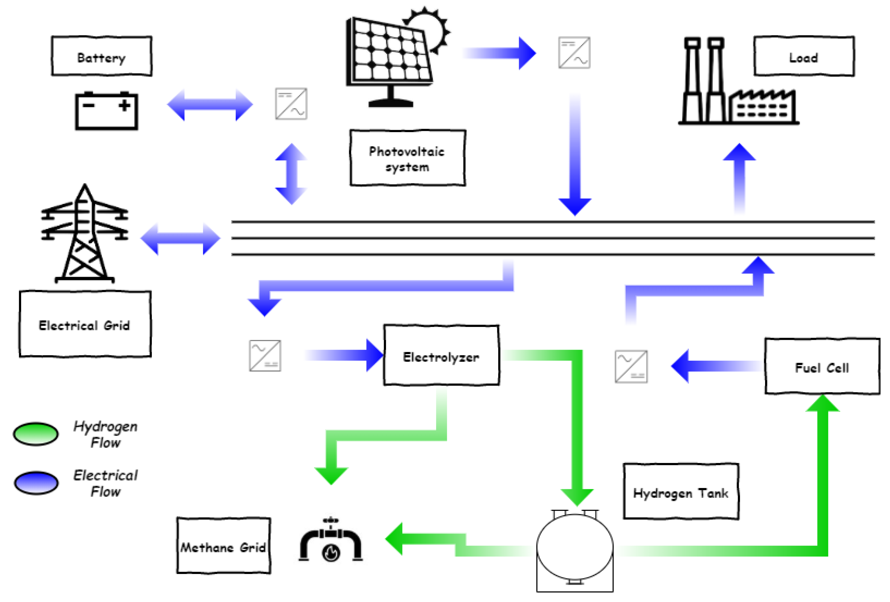
The Hybrid Energy System (HES) analysed in this work is made up of two different energy vectors: electricity and hydrogen. The primary energy source of the plant is solar irradiation while its outputs are electricity and hydrogen: electrical power can be consumed locally or sold to the electrical network. On the other hand, hydrogen produced by renewable electrical energy can be either converted again into electricity or sold to a natural gas network. Both forms of energy can be stored: in hydrogen tanks and/or in Battery Energy Storage System (BESS) accumulating electrical energy. In Figure 1, a sketch of the system and of its power flows is presented.

In the following, a brief outline of the methodology used and of the equations describing the working of modules are given.

2.1. Modelling of the HES

The modelling of the system is made on the basis of energy flow balance in time intervals over a time horizon defining the plant scheduling and management. The proposed simulation takes in input the power production and economical data, the characteristics of the power conversion modules and their interactions and as results it computes a strategy that minimises a target function by using output power levels as degrees of freedom of the system.

Basically, the workflow of the optimisation procedure is subdivided into three main sections:

• Definition of a scheduling interval and its discretisation. The number of intervals of equal length $\Delta t$ is $N_{int}$, for instance a one day scheduling period can be divided either into 24 intervals of 1 h or in 96 intervals of 15 min. Time profiles of the energy production such as production of the PV plant and demand of the local energy load, together with the time profiles of the energy prices, are considered to be known data. This phase is carried out by reading different files containing the time series of data, either obtained by environmental conditions (solar irradiation) or by market prices (purchasing and selling of electrical energy). As the approach proposed is more oriented toward energy flows, every power variable in the system is modelled as constant in each time interval. Transient phenomena, related for instance to power–electronics converters connecting PV output in DC and electrical grid in AC, are neglected and, furthermore, HES is considered to be in steady-state in each time interval.
• Definition of technical and operational characteristics of the different sources as well as connections among them. Mathematically, these constraint equations are divided into two categories:

  -

  Balance equations represent the energy balance of each energy carrier in order to ensure feasible solutions where output is covered by production.

  -

  Constitutive equations represent the relations between the input and output power of a source, as well as its operational limits.

  The first set of equation is linear by definition; its structure is in fact made up of an algebraic sum of energy values over a given time interval. Each energy vector is characterised by its own balance equation and a constraint equation is defined for every single time interval. The second set of equations does not have an a priori structure, as the input–output relation of one module could be in general a nonlinear function. In most application cases, these relations are linear or can be approximated by piece-wise linear relations.
• Computation of the target function to be optimised and evaluation of the scheduling strategy minimising/maximising it. As an example, if an economical target function is adopted, the sum over the time intervals of earnings obtained by selling the electrical energy to the grid has to be maximised. In this last case, the objective function is expressed as a linear form made by multiplying the energy sold to the grid in each interval by the unit selling price.

After the mathematical description of the HES is obtained, the optimisation of its target function can be attempted. This process can be approached in different ways, but, if model equations are linear, the most efficient way of looking for the optimal point is by using Linear Programming (LP) techniques. Unfortunately, the problem formulation is not fully linear because of the presence of piece-wise linear equations and/or by logical variables that must be used to describe the ON/OFF status of modules. In this case, the optimal scheduling can be found by means of a Mixed Integer Linear Programming (MILP) solver by using a standard branch and bound MILP solver [14]. A more detailed description of the procedure used can be found in [10] for the case of hybrid electric and thermal hybrid network.

2.2. PV Plant

The PV plant is modelled by means of its net power output in each time interval.

$$PV\left(t_k\right),k=1,\cdots ,N_{int}$$

(1)

The power takes into account the efficiency of DC/AC converters and transformers. The energy produced is given as $PV\left(t_k\right)\Delta t$ and it is expressed in ($\mathrm{MWh}$). The power produced is obtained by an atlas (e.g., [15]) and considering the PV modules technology and their fixed-mounting or single/double axis tracking.

2.3. Electrical Grid and Load

The plant is connected to the electrical grid with the possibility of selling and purchasing electrical energy. The main characteristics of the grid are the unit price values that change in time both during the day and throughout the year. These variations are expressed as a time series of the electrical prices. The unit selling price is given by:

$$c_s\left(t_k\right),k=1,\cdots ,N_{int}$$

(2)

$c_s$ coefficients are obtained by market data and are expressed in $(€/\mathrm{MWh})$. Electrical power can also be purchased by the grid at a unit price that is expressed by:

$$c_p\left(t_k\right)=c_s\left(t_k\right)+c_{grid}$$

(3)

where the constant term $c_{grid}$ takes into account the costs of electrical system charges, the fares for meter transport and management and excises and taxes which are added to the unit cost of electricity. Fixed costs of connections are not considered in the present work as they are independent from the plant management and they should be added afterwards.

Besides price values, the electrical connection is considered to have a maximum rated power $P_{grid}^{max}$ related to connecting lines and transformers capacities that cannot be exceeded.

The power level exchanged with the grid is one of the degrees of freedom of the plant management as power produced by PV plant can either be sold to the grid or, as shown below, stored in batteries or converted to hydrogen. In each time interval, the power exchanged with the grid is given by two variables, $P_s\left(t_k\right)$ and $P_p\left(t_k\right)$, the sold and purchased power values expressed in ($\mathrm{MW}$), respectively. The two variables are mutually exclusive as the plant cannot sell and purchase power at the same time. This constraint is taken into account by two logical variables that can take 0 or 1 values in each interval. The constraint equation is given by:

$$0\le {\delta }_s\left(t_k\right)+{\delta }_p\left(t_k\right)\le 1,k=1,\cdots ,N_{int}$$

(4)

which ensures that the plant in each $t_k$ can be either selling power $({\delta }_s\left(t_k\right)=1)$ or purchasing it $({\delta }_p\left(t_k\right)=1)$, or neither of the two. The presence of the logical variables in the problem formulation forces to use the MILP formulation for optimisation.

Another characteristic of the proposed formulation is the possibility to constrain the power exchanged with the electrical grid to follow a given profile in time. This need comes from the requirements of dispatching that can ask the plant to follow a schedule different from the production level of PV. The possibility of storing PV production in either BESS or hydrogen gives the plant more flexibility [16]. The modelling of this dispatch condition is, in the present formulation, managed by setting a logical variable ${\delta }_{disp}\left(t_k\right)$ at the 1 value in the time intervals when $P_s\left(t_k\right)$ or $P_p\left(t_k\right)$ must be equal to a set value $P_{grid}^{disp}\left(t_k\right)$.

Local electrical users can be present, and they are supposed to be known and defined for each time interval as:

$$U_e\left(t_k\right),k=1,\cdots ,N_{int}$$

(5)

2.4. Electrolyser

Water electrolysis is a viable technology to store electrical energy by converting it into hydrogen [17]. For what concerns the hydrogen production and avoiding details about the technology, the equation that describes water electrolysis is:

$$q_{el}\left(t_k\right)={\eta }_{el}·K_{el}·P_{el}\left(t_k\right)$$

(6)

where $q_{el}\left(t_k\right)$ is the hydrogen mass flow in the kth interval, expressed in $\mathrm{kg}/\mathrm{h}$; ${\eta }_{el}$ is the efficiency of the electrolyser which is considered constant and depending on the technology; $K_{el}$ is the operative constant that converts a unit electrical energy in input to the resulting hydrogen mass, for instance $K_{el}=21.25\mathrm{kg}/\mathrm{MWh},(@273\mathrm{K},1\mathrm{bar})$; and $P_{el}\left(t_k\right)$ is the electrical power in input to the electrolyser in the kth interval and it is considered as the independent variable of the component.

By stoichiometry, the water mass needed to obtain a hydrogen unit mass in $\mathrm{kg}$ is given by:

$$m_{H2O}=9·m_{H2}$$

(7)

Following the approach proposed in [8], the operative cost for running the electrolyser is computed on a depreciation approach. To this cost a maintenance cost is added. the equation used is:

$$c_{el}=\frac{C_{e{l}_i}}{L_{el}}+c_{e{l}_m}$$

(8)

where $C_{e{l}_i}=c_{e{l}_i}·P_{e{l}_{max}}$, expressed in €, is the electrolyser investment cost and $c_{e{l}_i}$, in €$/\mathrm{kW}$, is its unit cost; $L_{el}$, expressed in $\mathrm{h}$, is the service life; and $c_{e{l}_m}$, expressed in €$/\mathrm{h}$, is the hourly operation and maintenance (O&M) cost.

2.5. Fuel Cell

Fuel cell is the power module that converts hydrogen in electrical power [18]. As for the electrolyser, its operating equation is given by:

$$q_{fc}\left(t_k\right)=\frac{P_{fc}\left(t_k\right)}{{\eta }_{fc}·H_i}$$

(9)

where $P_{fc}\left(t_k\right)$ is the electrical power in input to the fuel cell and it is its control variable; $q_{fc}\left(t_k\right)$ is the hydrogen mass flow in the kth interval, expressed in $\mathrm{kg}/\mathrm{h}$, in input to the fuel cell; ${\eta }_{FC}$ is the efficiency of the fuel cell that is considered constant and depending on the technology; and $H_i$ is its operating constant, for instance $H_i=0.033$, expressed in $\mathrm{MWh}/\mathrm{kg},(@273\mathrm{K},1\mathrm{bar})$.

Again, as for electrolyser, economic costs are evaluated on a depreciation basis:

$$c_{fc}=\frac{C_{f{c}_i}}{L_{fc}}+c_{f{c}_m}$$

(10)

where $C_{f{c}_i}=c_{f{c}_i}·P_{f{c}_{max}}$, in €, is the investment cost and $c_{f{c}_i}$, in €$/\mathrm{kW}$, is the unit power cost; $L_{fc}$, $\mathrm{h}$, is the service life; and $c_{f{c}_m}$, in €$/\mathrm{h}$

2.6. Hydrogen Tank

The mass of hydrogen coming from water electrolysis can be stored in a tank to be used, at a later time, by fuel cell. The quantity of hydrogen mass stored in the tank is ruled by a dynamic equation as its rate of variation depends on the mass flow in input/output respectively from electrolyser/fuel cell. It is in fact given by:

$$M_{tank}\left(t_k\right)=M_{tank}\left(t_{k-1}\right)+\frac{(q_{tank}^{in}\left(t_k\right)-q_{tank}^{out}\left(t_k\right))}{M_{tank}^{max}}·\Delta t·100$$

(11)

where $q_{tank}^{in}\left(t_k\right)$, in $\mathrm{kg}/\mathrm{h}$ is the hydrogen mass flow in input to the tank, while $q_{tank}^{out}\left(t_k\right)$ is the outgoing flow; and $M_{tank}\left(t_k\right)$ is the quantity of stored hydrogen, expressed as a percentage of the maximum mass that the tank can contain $M_{tank}^{max}$ in $\mathrm{kg}$. As in previous cases, economic costs are computed on a depreciation basis:

$$c_{tank}=\frac{C_{tan{k}_i}}{L_{tank}}+c_{tan{k}_m}$$

(12)

where $C_{tan{k}_i}=c_{tan{k}_i}·M_{tank}^{max}$, in € is the tank investment cost and $c_{tan{k}_i}$ in €$/\mathrm{kg}$ is the unit cost; $L_{tank}$, in $\mathrm{h}$ is the service life; and $c_{tan{k}_m}$, in €$/\mathrm{h}$, is the hourly operation and maintenance (O&M) cost.

2.7. Natural Gas Grid

Hydrogen can be transported employing the same infrastructures already developed for natural gas as it can be blended up to a certain percentage, usually lower than 10 %, with natural gas [19]. In the present model, the hydrogen mass flow sold to the gas grid is expressed by $q_{grid}\left(t_k\right)$, in $\mathrm{kg}/\mathrm{h}$. The unit selling price of hydrogen, expressed in €$/\mathrm{kg}$, is taken as a datum known from natural gas market. Once the unit price is defined, the decision variable $q_{grid}\left(t_k\right)$, expressed in $\mathrm{kg}/\mathrm{h}$, is used to describe hydrogen flow to the natural gas grid.

2.8. Battery Energy Storage System

Storage of electrical energy can be obtained by electrochemical batteries. This form of storage is alternative to hydrogen conversion. As in the case of hydrogen storage, the equation that models this phenomenon is dynamic as the rate of energy storage is equal to the battery power input/output.

The BESS status is described by its State Of Charge (SOC) that can be expressed as a percentage of the maximum battery capacity. The equation describing the BESS is:

$$So{c}_{batt}\left(t_k\right)=So{c}_{batt}\left(t_{k-1}\right)+\frac{(P_{bc}\left(t_k\right)·{\eta }_{bc}-\frac{P_{bd}\left(t_k\right)}{{\eta }_{bd}})}{E_{batt}}·\Delta t·100$$

(13)

where $P_{bc}\left(t_k\right)$, in $\mathrm{MW}$ is the electrical power flowing in (charging) the battery; $P_{bd}\left(t_k\right)$, in $\mathrm{MW}$ is the electrical power flowing out (discharging) the battery; ${\eta }_{bc}$ and ${\eta }_{bd}$ are the charging and discharging efficiency values; and $E_{batt}$, in $\mathrm{MWh}$, is the rated battery capacity.

Again, the depreciation approach is used for the definition of the economic cost, while, in this case, maintenance costs are neglected [8]. The number of charge/discharge cycles is used to evaluate the service life of BESS.

3. MILP Optimisation Procedure

The mathematical model above defined can be used to describe the HES and to optimise it. The decision variables used in the problem are subdivided into real valued (

Table 1. Real valued decision variables.

Name	Unit	Description	Carrier
$P_{el}$	$\mathrm{MW}$	electrolyser input power	electrical
$P_{fc}$	$\mathrm{MW}$	Fuel Cell output power	electrical
$P_{bc}$	$\mathrm{MW}$	BESS charging power	electrical
$P_{bd}$	$\mathrm{MW}$	BESS discharging power	electrical
$P_s$	$\mathrm{MW}$	power sold to the grid	electrical
$P_p$	$\mathrm{MW}$	power purchased from the grid	electrical
$q_{grid}$	$\mathrm{kg}/\mathrm{h}$	mass flow sold to the gas grid	hydrogen
$q_{tank}^{in}$	$\mathrm{kg}/\mathrm{h}$	mass flow in the tank	hydrogen
$q_{tank}^{out}$	$\mathrm{kg}/\mathrm{h}$	mass flow out of the tank	hydrogen

) and integer (0/1) ones (

Table 2. Integer valued decision variables.

Name	Description
${\delta }_{el}$	electrolyser status
${\delta }_{fc}$	Fuel Cell status
${\delta }_s$	electrical sell
${\delta }_p$	electrical purchase
${\delta }_{bc}$	BESS charge
${\delta }_{bd}$	BESS discharge
${\delta }_{grid}$	hydrogen sell to gas grid
${\delta }_{in}$	hydrogen tank in flow
${\delta }_{out}$	hydrogen tank out flow

). The total number of variables for each time interval is thus nine real variables and nine integer ones.

3.1. Electrical Balance

In every time interval, the balance of electrical power must be enforced, that is:

$$\left.\begin{array}{c}PV\left(t_k\right)-U_e\left(t_k\right)·\Delta t+\hfill \\ +P_p\left(t_k\right)·\Delta t-P_s\left(t_k\right)·\Delta t+\hfill \\ -P_{el}\left(t_k\right)·\Delta t+P_{fc}\left(t_k\right)·\Delta t+\hfill \\ -P_{bc}\left(t_k\right)·\Delta t+P_{bd}\left(t_k\right)·\Delta t=0\hfill \end{array}\right\}k=1,\cdots ,N_{int}$$

(14)

Besides balance equation, limits on power values must also be constrained:

$$0\le P_{bc}\left(t_k\right)\le {\delta }_{bc}\left(t_k\right)·P_{b{c}_{max}}$$

(15)

$$0\le P_{bd}\left(t_k\right)\le {\delta }_{bd}\left(t_k\right)·P_{b{d}_{max}}$$

(16)

$$0\le P_s\left(t_k\right)\le {\delta }_s\left(t_k\right)·P_{s_{max}}$$

(17)

$$0\le P_p\left(t_k\right)\le {\delta }_p\left(t_k\right)·P_{p_{max}}$$

(18)

$${\delta }_{el}\left(t_k\right)·P_{e{l}_{min}}\le P_{el}\left(t_k\right)\le {\delta }_{el}\left(t_k\right)·P_{e{l}_{max}}$$

(19)

$${\delta }_{fc}\left(t_k\right)·P_{f{c}_{min}}\le P_{fc}\left(t_k\right)\le {\delta }_{fc}\left(t_k\right)·P_{f{c}_{max}}$$

(20)

$$So{c}_{min}\le Soc\left(t_k\right)\le So{c}_{max}$$

(21)

in addition, physical constraints on some variables must also be defined to avoid conflicts between power flows, as previously explained in (4):

$$0\le {\delta }_{el}\left(t_k\right)+{\delta }_{fc}\left(t_k\right)\le 1$$

(22)

$$0\le {\delta }_s\left(t_k\right)+{\delta }_p\left(t_k\right)\le 1$$

(23)

$$0\le {\delta }_{bc}\left(t_k\right)+{\delta }_{bd}\left(t_k\right)\le 1$$

(24)

Initial and final conditions of storage units can be specified, for instance imposing that start and end status of storage would be equal:

$$\sum _{k=1}^{N_p}[P_{bc}\left(t_k\right)-P_{bd}\left(t_k\right)]=0$$

(25)

3.2. Hydrogen Balance

In addition, the hydrogen balance must be imposed in each time interval. By considering as positive the hydrogen generated, the equation is:

$$\left.\begin{array}{c}+q_{el}\left(t_k\right)·\Delta t-q_{fc}\left(t_k\right)·\Delta t-q_{grid}\left(t_k\right)·\Delta t+\hfill \\ -q_{tank}^{in}\left(t_k\right)·\Delta t+q_{tank}^{out}\left(t_k\right)·\Delta t=0\hfill \end{array}\right\}k=1,\cdots ,N_{int}$$

(26)

As in the previous case, for hydrogen constraints on maximum values of flows, contemporary in and out flows and initial and final status of storage must also be enforced, so that:

$$0\le q_{grid}\left(t_k\right)\le {\delta }_{grid}\left(t_k\right)·q_{grid}^{max}$$

(27)

$$0\le q_{tan{k}_{in}}\left(t_k\right)\le {\delta }_{in}\left(t_k\right)·q_{tank}^{max}$$

(28)

$$0\le q_{tan{k}_{out}}\left(t_k\right)\le {\delta }_{out}\left(t_k\right)·q_{tank}^{max}$$

(29)

$$M_{tank}^{min}\le M_{tank}\left(t_k\right)\le M_{tank}^{max}$$

(30)

$$0\le {\delta }_{in}\left(t_k\right)+{\delta }_{out}\left(t_k\right)\le 1$$

(31)

$$\sum _{k=1}^{N_p}[q_{tan{k}_{in}}\left(t_k\right)-q_{tan{k}_{out}}\left(t_k\right)]=0$$

(32)

3.3. Objective Function

The aim of the procedure is to find out the better exploitation for the electrical power produced by PV considering all alternatives regarding storage. The objective function is in this case economical: all earning and costs during the scheduling period are considered, so that the problem is formulated by:

$$\sum _{k=1}^{N_p}min\left\{\begin{array}{c}+c_{el}·{\delta }_{el}\left(t_k\right)·\Delta t+c_{fc}·{\delta }_{fc}\left(t_k\right)·\Delta t+\hfill \\ -c_s\left(t_k\right)·P_s\left(t_k\right)·\Delta t+c_p·P_p\left(t_k\right)·\Delta t+\hfill \\ -c_{H_2}·q_{grid}\left(t_k\right)·\Delta t+c_{tank}·\Delta t+\hfill \\ +c_{bc}·P_{bc}\left(t_k\right)·\Delta t+c_{bd}·P_{bd}\left(t_k\right)·\Delta t\hfill \end{array}\right.$$

(33)

The objective function must be minimised taking into account all constraints presented in the previous sections.

By considering the list of variables presented in Table 1 and Table 2, the problem has a dimension that is $18\ast N_{int}$; for example, for a week period scheduling discretised on the hour basis $N_{int}=168$, the problem has to handle 1512 real valued variables and 1512 integer valued ones.

4. Case Studies

The proposed optimisation formulation was implemented in a Python procedure [20], using the package PuLP [21] for the solution of the MILP problem. The simulation was implemented with a modular architecture so that components can be added or removed from the system, testing different plant configurations. In this way, several arrangements were run with the aim of checking procedure functionality and accuracy. These case studies were inspired by a real test case situated in the central part of Italy where there is the possibility of building a large-scale PV plant on poor quality agricultural land in a region easily accessed by electrical, natural gas and water infrastructures. Irradiation data on this location were then used to draw a PV and hydrogen plant. The V plant was designed on state-of-the-art panels coupled with hydrogen handling components defined on the basis of literature data, mainly the ones found in [8]. The performance of the plant were evaluated on different time horizons, as described below. For the sake of simplicity and graphical clarity, one day scheduling period on the hour basis was used in all the presented cases. The day used for display was sampled in April as, from analysis of different seasonal data, it is the one where energy storage is more often used.

4.1. Computational Cost

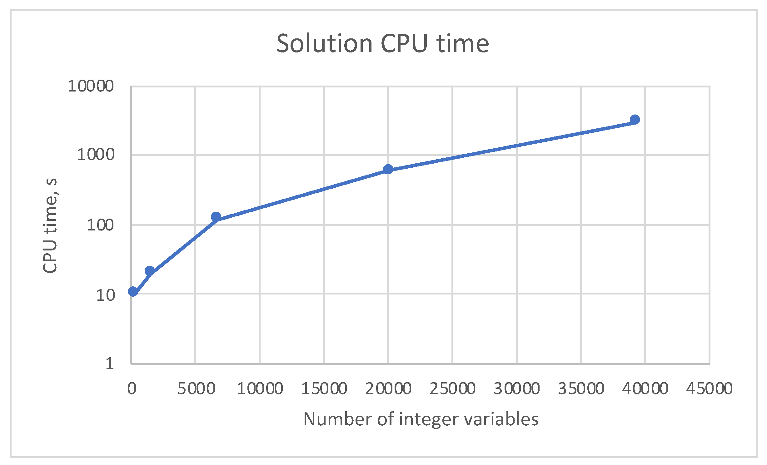
The computational cost of the procedure was tested to verify its applicability to real world cases. The procedure was run on a computer with 2.5 GHz Dual-Core Intel Core i7 running different problems changing the dimension in terms of number of variables. CPU times were recorded and are reported in

Table 3. CPU time on one-hour time scale discretisation.

Scheduling	Number of Variables Real	Number of Variables Integer	Number of Constraints	CPU Time ($\mathbf{s}$)
one day	216	216	170	10
one week	1512	1512	1190	20
one month	6696	6696	5270	120
three months	20,088	20,088	15,810	600
six months	39,312	39,312	31,620	3000

. The CPU times are also shown in semi-logarithmic scale in Figure 2. This representation highlights the exponential nature of the computational cost of the procedure [22]. Despite this exponential cost, it must be remarked that the problem has a weak coupling between time intervals as only storage devices are characterised by dynamic equations, e.g., (11) and (13). Following the experience gained with other scheduling optimisation processes, the most interesting analysis period is usually one day or one week. Thus, in absolute terms, the computational costs for operational cases, i.e., 24 or 168 h for one day or one week, respectively, at the hour base, are well matched with the use of the procedure within an operational optimisation of the system.

4.2. Case 1: Connection with Natural Gas Grid

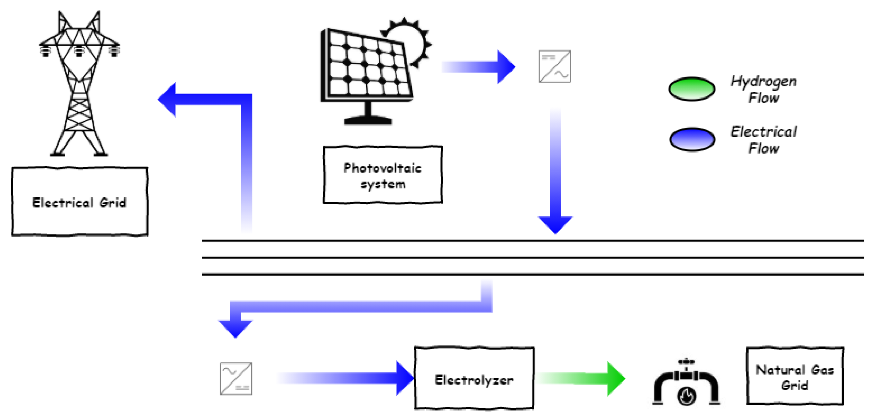
In this case, the interactions between the HES and natural gas grid are considered and thus only the electrolyser is working in the system while hydrogen tank and fuel cell are removed. The aim of this study is to find out the selling price of hydrogen to the natural gas grid that makes the hydrogen generation competitive versus the selling of the PV production to the electrical grid. A schematic outline of the HES is shown in Figure 3.

The following data are considered for the plant:

-

PV plant:

$$P{V}_{rate}=120\mathrm{MW}$$

(34)

-

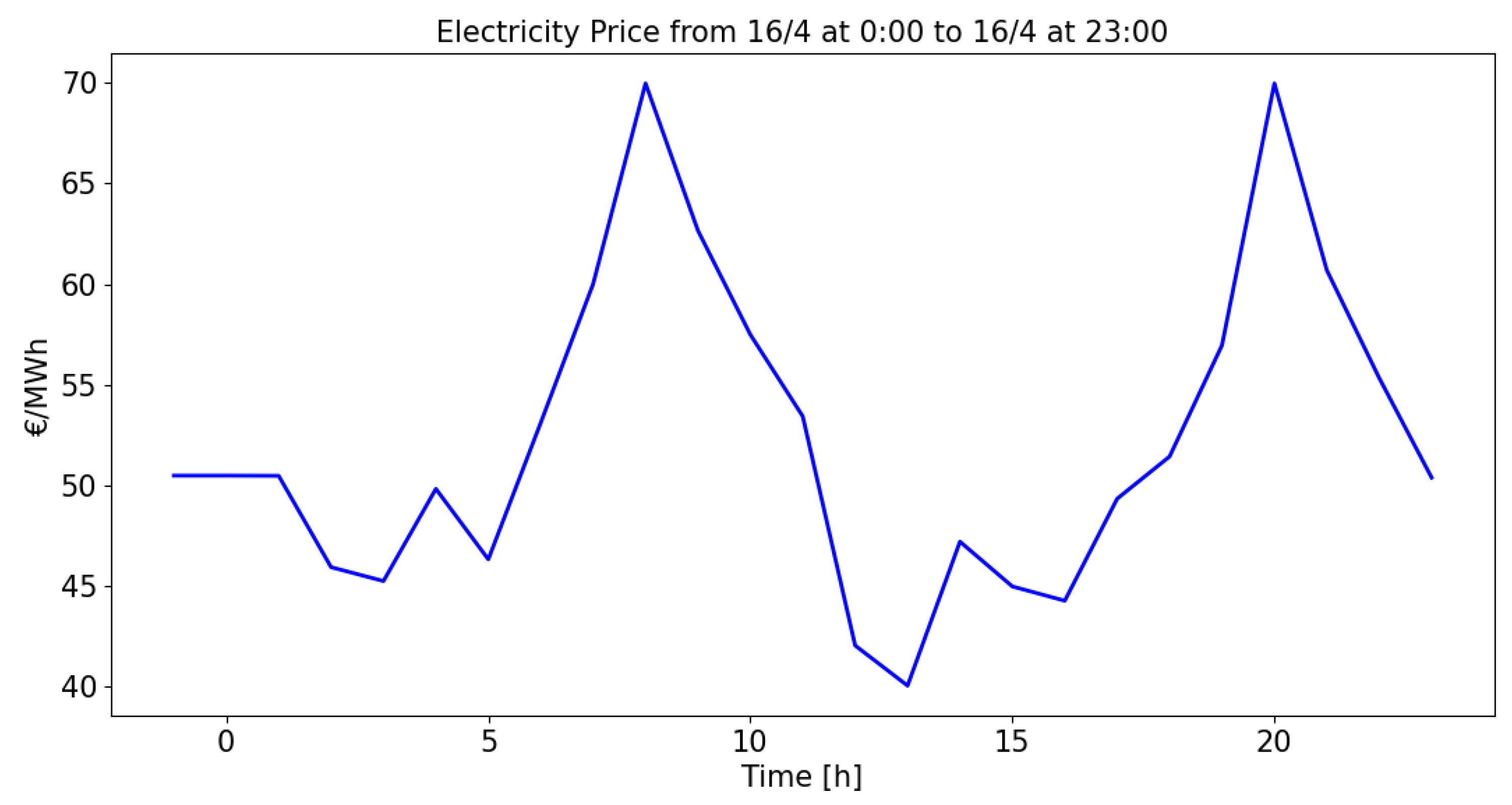
Electrical network:

$$P_{grid}^{max}=200\mathrm{MW}$$

(35)

The unit price of electricity is defined on the basis of market data and one day series is reported in Figure 4.

-

Electrolyser:

$$P_{e{l}_{max}}=20\mathrm{MW}$$

(36)

$$P_{e{l}_{min}}=20\%·P_{e{l}_{max}}=4\mathrm{MW}$$

(37)

$${\eta }_{el}=0.7$$

(38)

$$c_{el}=160.00€/\mathrm{h}$$

(39)

It is considered that hydrogen is produced at the pressure of $30\mathrm{bar}$, which is suitable for natural gas grid output and for short term storage.

-

Natural gas grid:

$$q_{grid}^{max}=1000\mathrm{kg}/\mathrm{h}$$

(40)

The hydrogen selling price is set as fixed externally.

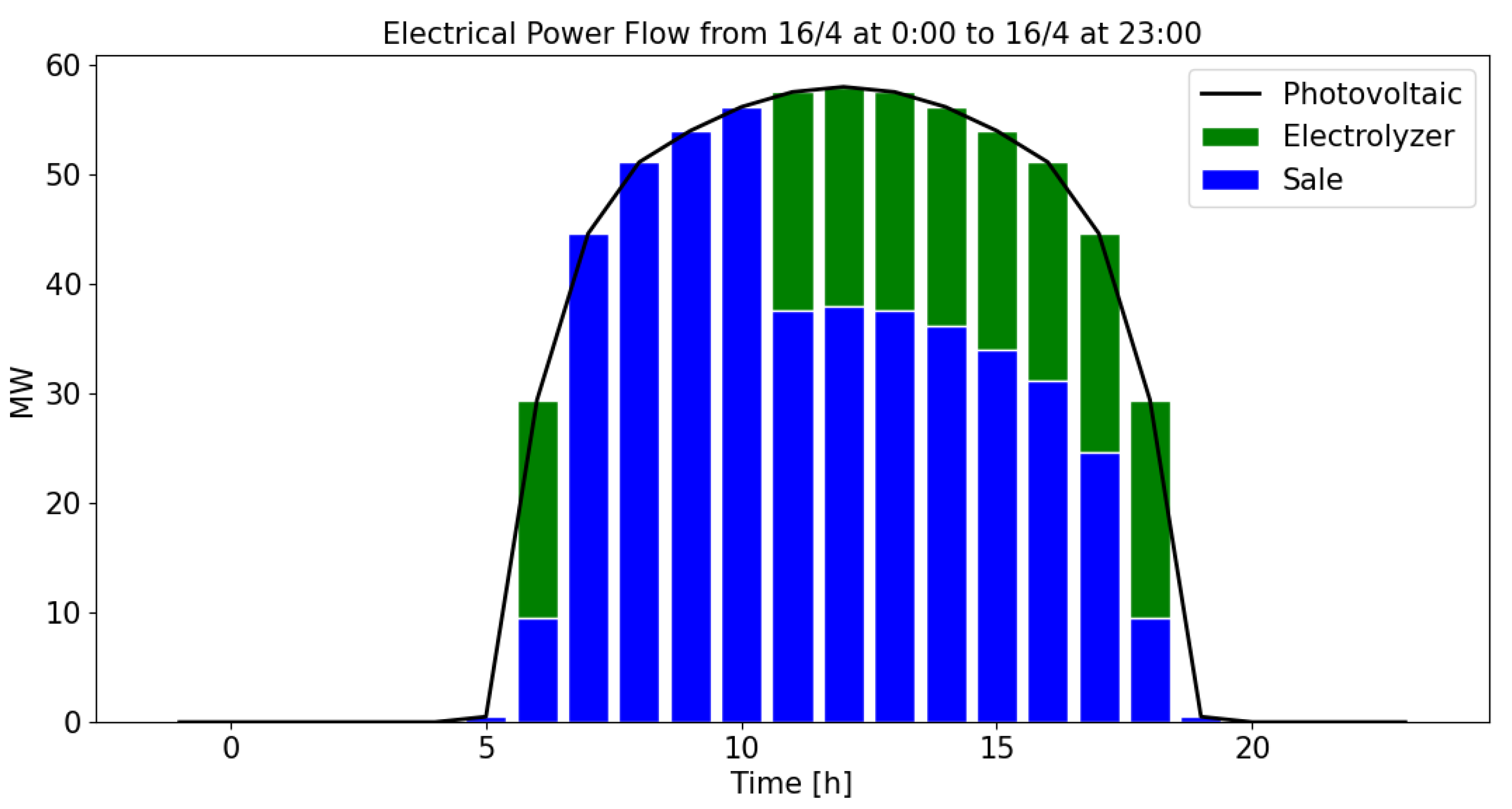
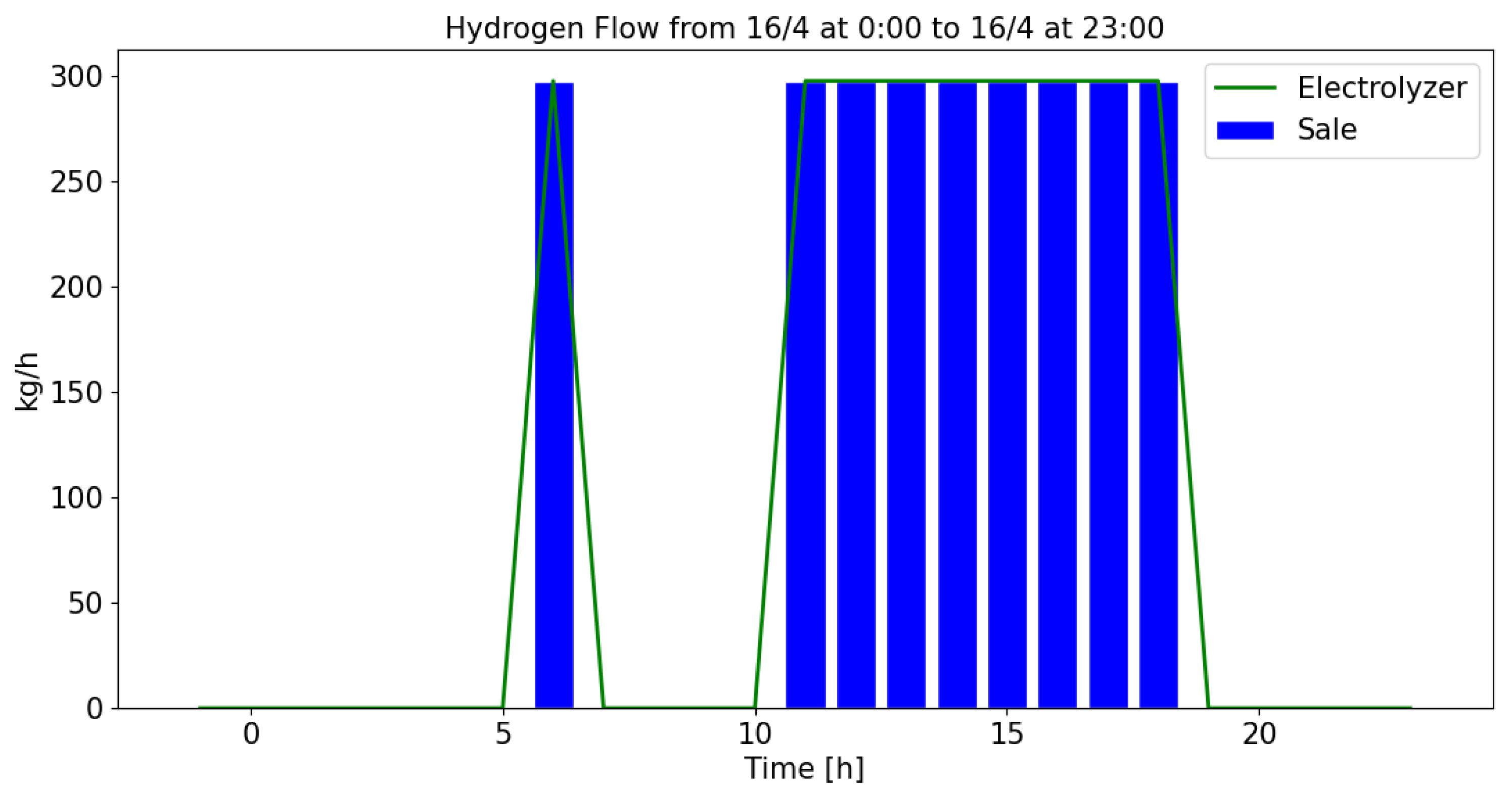
Hydrogen selling price is used as a parameter varying within 2–5 €$/\mathrm{kg}$. The results obtained by the optimiser in one sample day in April, at the selling hydrogen price of $4.2€/\mathrm{kg}$, are shown in Figure 5 and Figure 6. It is possible to see how the competition between the electricity and natural gas prices makes more convenient to produce hydrogen in low electrical price hours. In particular, the solution found exploits 1 h during the very early morning and the interval between 11 and 19, when the electricity price is constrained to be low by a large offer of PV renewable energy available on the electrical market.

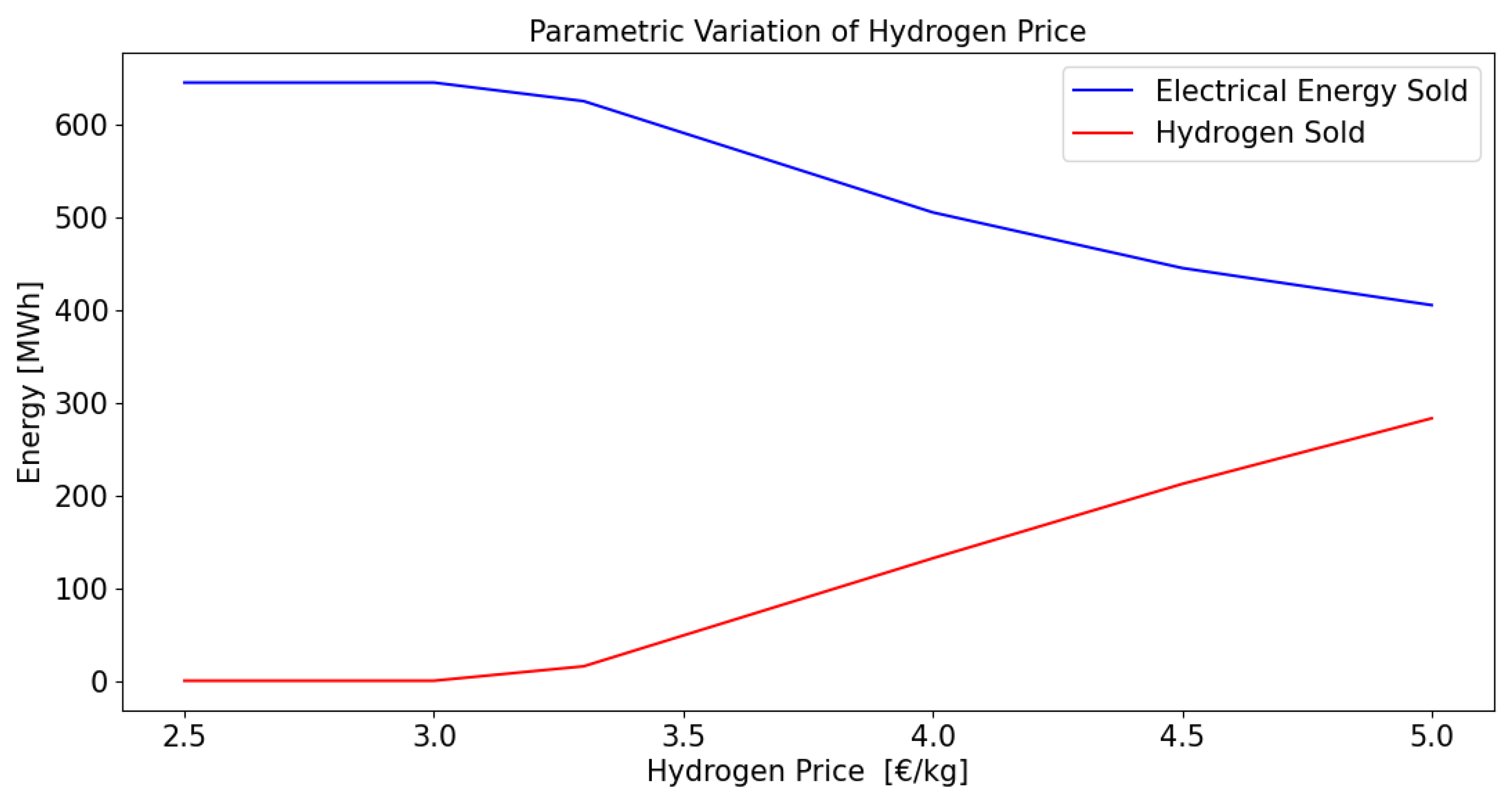
From the parametric analysis, it is possible to find the hydrogen selling price for which, during the day, it is competitive to produce hydrogen. By considering a 24-h scheduling period and by varying the hydrogen price, the quantity of hydrogen energy produced and sold to the natural gas grid is shown in Figure 7 and numerical values are reported in

Table 4. Daily energy sold under the form of electricity and hydrogen.

${\mathit{H}}_2$ Price	Electrical Energy	${\mathit{H}}_2$ Energy
$€/\mathrm{kg}$	$\mathrm{MWh}$	$\mathrm{MWh}$
2.5	645.3	0.0
3.0	645.3	0.0
3.3	625.2	17.7
4.0	505.6	130.3
4.5	445.9	214.3
5.0	405.9	284.2

. It can be seen that the breakeven price, defined as the gas price at which, with the present situation of electrical market price, the production of hydrogen starts to be competitive, is found at about $3€/\mathrm{kg}$. This is due to a low price of electrical energy during the central hours of the day, as can it be seen in Figure 4.

4.3. Case 2: Hydrogen Storage and Fuel Cell Generation

The production of electrical power by the fuel cell requires a double stage of power conversion: from electrical to hydrogen and back from hydrogen to electrical. This process is obviously largely inefficient due to the sum of the losses in both energy conversion processes. Under these hypothesis and considering the current values of energy prices, the production of electrical energy by the fuel cell is not competitive. To test the procedure, an academic test case was devised which requires the triggering of the fuel cell, thus validating the correctness of the whole simulation.

The electrolyser, tank and grid data are the same as used in Case 1. The fuel cell has the following data:

$$P_{f{c}_{max}}=5\mathrm{MW}$$

(41)

$$P_{f{c}_{min}}=20\%·P_{f{c}_{max}}=4\mathrm{MW}$$

(42)

$${\eta }_{fc}=0.7$$

(43)

$$c_{fc}=45.00€/\mathrm{h}$$

(44)

In this case, the hydrogen tank has a maximum capacity of $M_{tank}^{max}=350\mathrm{kg}$ leading to a maximum value of stored energy equal to $11.55\mathrm{MWh}$, which is sufficient for a short-term storage even if it cannot provide long self-sufficiency periods of the plant.

This test is made by a specific arrangement: it is considered that a local electrical load, constant in time, and with a power $U_e=1\mathrm{MW}$, is connected to the plant. This load is supplied during the day by the electrical power produced by PV while during the night it can be provided either by the power purchased by the electrical grid or by the fuel cell. When the cost of purchasing electrical power during the night overcomes a certain threshold, it is more convenient for the system to accumulate hydrogen during the day and use it in the night by running the fuel cell. To simplify the analysis, a flat cost of electrical energy is used; this assumption again does not correspond to the actual situation of prices, but it is used here for testing purposes.

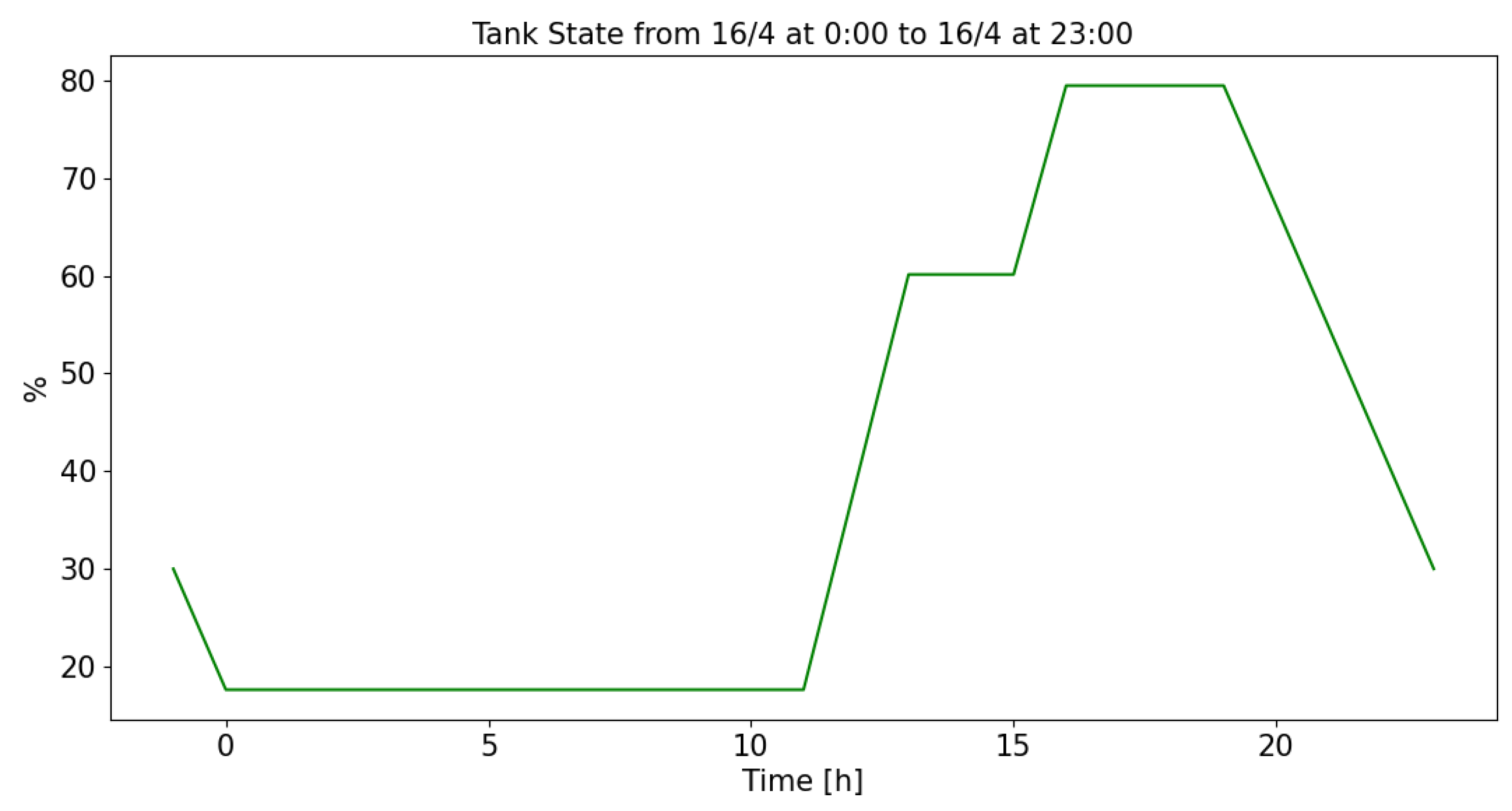
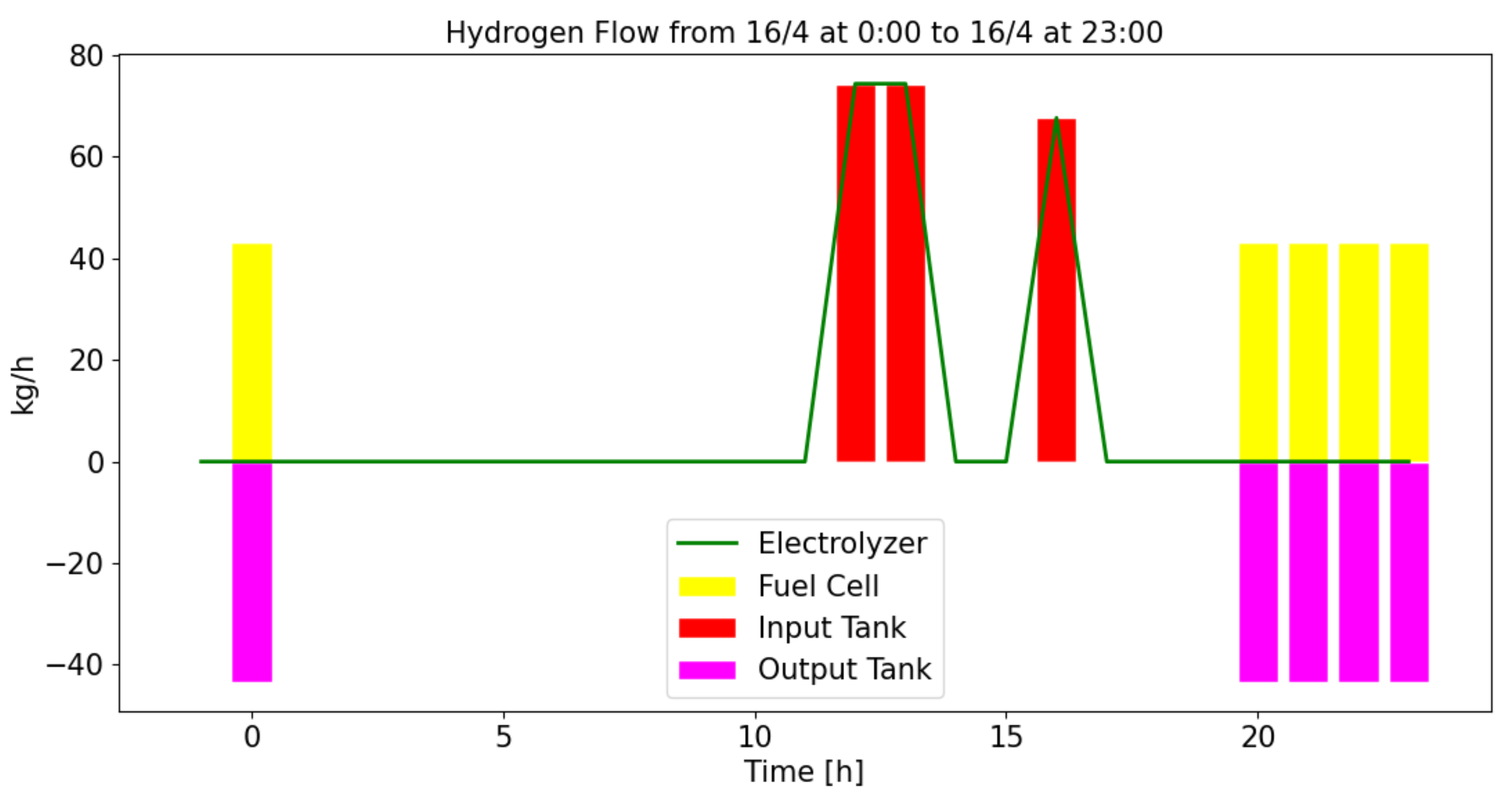
By changing parametrically the price of electricity, the procedure finds it more convenient to run the fuel cell for a value larger than $200€/\mathrm{MWh}$. As displayed in Figure 8, the hydrogen tank is filled up during the day by means of the PV energy. During evening and night, the fuel cell is running until the hydrogen tank is emptied so that, in this particular case, the load is supplied for 5 h, as shown in Figure 9. As the capacity of the tank is limited, the procedure finds during the day the hours when it is less convenient selling electrical power to the grid and stores it instead in the hydrogen tank.

Besides the testing of the procedure, the breakeven price value of $200€/\mathrm{MWh}$ gives a term of comparison with the present price situation with respect to the one when the local use of hydrogen is becoming economically suited.

4.4. Case 3: Dispatching Constraint

Non-predictable renewable energy has an impact on power delivery scheduling and can overload the transmission system [23,24]. In this respect, energy storage of PV electricity in hydrogen and its subsequent conversion in electrical energy can help ancillary electrical grid systems.

This aspect is modelled in the scheduling procedure by activating a constraint that affects the value of power exchanged by the system with the electrical grid. If HES is licensed as a controllable power generation unit, it is characterised by a power band which can be increased or reduced so that the power exchanged with the electrical grid exactly match a time profile. This service is remunerated by the Transmission System Operator by means of a power band price defined in the regulation markets.

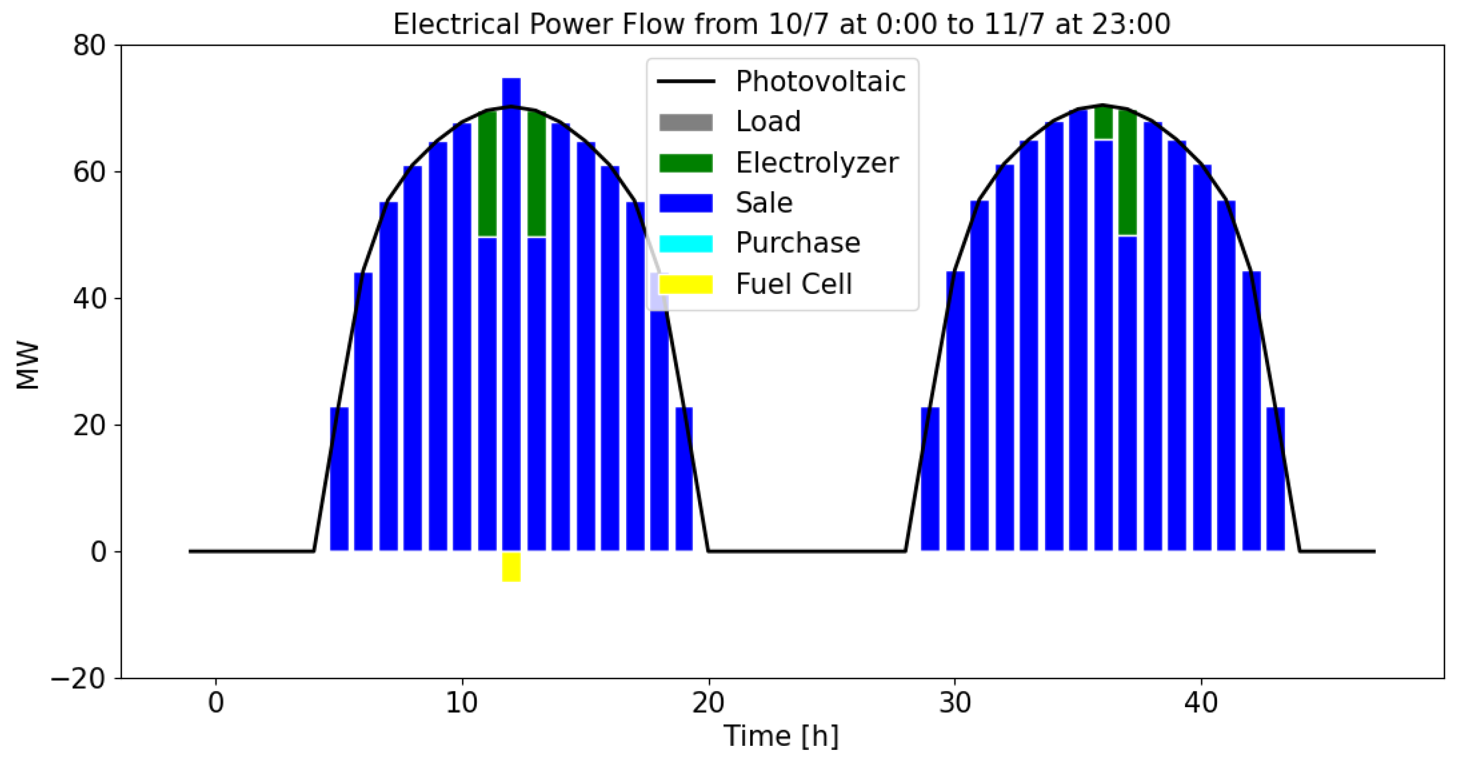
The procedure is tested in this case by simulating two days of scheduling with two dispatch requests. On the first day, an increase in power output for 1 h, at 11 a.m., is required: $75\mathrm{MW}$ is asked while the PV production is forecasted at $70\mathrm{MW}$. On the second day, a reduction of power output is imposed: power sold to the grid is reduced from $70\mathrm{MW}$ of forecasted PV to $65\mathrm{MW}$, again for a period of 1 h. The procedure is able to find an optimal solution by adding the fuel cell output to the PV production in the first case while storing the excess power in hydrogen in the second. The solution of the MILP formulation assures that a feasible solution fulfilling the limits imposed by storage capacity can be found. A hourly diagram of the quantities involved is shown in Figure (Figure 10).

This means that there is either sufficient energy stored, or capacity to store it, to meet the dispatch constraint, otherwise the optimisation run exits with an unfeasible status. In addition, the scheduling is optimal in the sense that, besides fulfilling the power output required, the minimum operating cost is sought as required by problem definition in Equation (33).

5. Discussion and Further Developments

The proposed MILP-based procedure was applied to several cases of operational optimisation of a HES with PV generation and hydrogen conversion facilities. The procedure enabled the definition of minimum operational costs which can be used both for the evaluation of several economic indicators in the planning phase of HES and/or for runtime scheduling of existing plants.

The procedure can in fact be applied, for instance, to the evaluation of key performance indices (for instance the Levelised Cost Of Energy produced by the plant) assuring the minimisation of its operational costs under the dynamic price variation and fulfilment of all technical constraints. Parametric studies can be performed by changing the parameters of the system, both technical and economical, in order to find their best arrangement in a planning phase of the HES or to find its operational scheduling on an existing system.

Further developments of the procedure are related to the addition of more criteria for optimisation, allowing the introduction of complex storage models, for instance taking into account battery ageing, and of environmental quantities such as the saving of greenhouse gas emissions. In this case, the role of hydrogen in industrial or transport applications could be assessed. These new features would allow critically evaluating different scenarios where hydrogen requests from particular applications are inserted and/or further constraints are considered, for instance limitation on water availability in input to the electrolyser or additional costs on storage of hydrogen and its liquefaction process.

References

- Communication from the Commission to the European Parliament, the Council, the European Economic and Social Committee and the Committee of the Regions. A Hydrogen Strategy for a Climate-Neutral Europe; Brussels, 8.7.2020 COM(2020) 301 Final. Available online: https://ec.europa.eu/knowledge4policy/publication/ (accessed on 10 July 2020).
- Hybrid Energy Networks: District Heating and Cooling Networks in an Integrated Energy System Context. Available online: https://www.iea-dhc.org/the-research/annexes/2017-2021-annex-ts3-draft/ (accessed on 1 July 2020).
- Ball, M.; Wietschel, M. The future of hydrogen-opportunities and challenges. Int. J. Hydrogen Energy 2009, 34, 615–627. [Google Scholar] [CrossRef]
- Fairley, P. Solar and Wind Power Could Ignite a Hydrogen Energy Comeback. Sci. Am. 2020, 322, 36–43. [Google Scholar]
- Lund, H.; Werner, S.; Wiltshire, R.; Svendsen, S.; Thorsen, J.E.; Hvelplund, F.; Mathiesen, B.V. 4th Generation District Heating (4GDH): Integrating smart thermal grids into future sustainable energy systems. Energy 2014, 68, 1–11. [Google Scholar] [CrossRef]
- Su, W.; Wang, J.; Roh, J. Stochastic Energy Scheduling in Microgrids With Intermittent Renewable Energy Resources. IEEE Trans. Smart Grid 2014, 5, 1876–1883. [Google Scholar] [CrossRef]
- Clegg, S.; Mancarella, P. Integrated Modeling and Assessment of the Operational Impact of Power-to-Gas (P2G) on Electrical and Gas Transmission Networks. IEEE Trans. Sustain. Energy 2015, 6, 1234–1244. [Google Scholar] [CrossRef]
- Yang, H.; Pu, Y.; Qiu, Y.; Li, Q.; Chen, W. Multi-Time Scale Integration of Robust Optimization with MPC for Islanded Hydrogen-Based Microgrid. In Proceedings of the 2019 IEEE Sustainable Power and Energy Conference (iSPEC), Beijing, China, 21–23 November 2019; pp. 1163–1168. [Google Scholar]
- Rodriguez del Nozal, A.; Gutierrez Reina, D.; Alvarado-Barrios, L.; Tapia, A.; Esca no, J.M. A MPC Strategy for the Optimal Management of Microgrids Based on Evolutionary Optimization. Electronics 2019, 8, 1371. [Google Scholar] [CrossRef] [Green Version]
- Canova, A.; Cavallero, C.; Freschi, F.; Giaccone, L.; Repetto, M.; Tartaglia, M. Optimal energy management. IEEE Ind. Appl. Mag. 2009, 15, 62–65. [Google Scholar] [CrossRef]
- Freschi, F.; Giaccone, L.; Lazzeroni, P.; Repetto, M. Economic and environmental analysis of a trigeneration system for food-industry: A case study. Appl. Energy 2013, 107, 157–172. [Google Scholar] [CrossRef]
- Teng, F.; Strbac, G. Full Stochastic Scheduling for Low-Carbon Electricity Systems. IEEE Trans. Autom. Sci. Eng. 2017, 14, 461–470. [Google Scholar] [CrossRef]
- Zhang, X.; Strbac, G.; Shah, N.; Teng, F.; Pudjianto, D. Whole-System Assessment of the Benefits of Integrated Electricity and Heat System. IEEE Trans. Smart Grid 2019, 10, 1132–1145. [Google Scholar] [CrossRef]
- Cook, W.; Koch, T.; Steffy, D.; Wolter, K. An Exact Rational Mixed-Integer Programming Solver. In Lecture Notes in Computer Science (LNCS); Springer: Berlin/Heidelberg, Germany, 2011; pp. 104–116. [Google Scholar]
- Photovoltaic Geographical Information System (PVGIS). Available online: http://re.jrc.ec.europa.eu/pvgis/ (accessed on 1 July 2020).
- Teleke, S.; Baran, M.E.; Bhattacharya, S.; Huang, A.Q. Rule-Based Control of Battery Energy Storage for Dispatching Intermittent Renewable Sources. IEEE Trans. Sustain. Energy 2010, 1, 117–124. [Google Scholar] [CrossRef]
- Carmo, M.; Fritz, D.L.; Mergel, J.; Stolten, D. A comprehensive review on PEM water electrolysis. Int. J. Hydrogen Energy 2013, 38, 4901–4934. [Google Scholar] [CrossRef]
- Vazquez, S.; Lukic, S.M.; Galvan, E.; Franquelo, L.G.; Carrasco, J.M. Energy Storage Systems for Transport and Grid Applications. IEEE Trans. Ind. Electron. 2010, 57, 3881–3895. [Google Scholar] [CrossRef] [Green Version]
- Quarton, C.J.; Samsatli, S. Power-to-gas for injection into the gas grid: What can we learn from real-life projects, economic assessments and systems modelling? Renew. Sustain. Energy Rev. 2018, 98, 302–316. [Google Scholar] [CrossRef]
- Available online: https://www.python.org (accessed on 1 July 2020).
- Available online: http://citeseerx.ist.psu.edu/viewdoc/summary?doi=10.1.1.416.4985’ (accessed on 1 July 2020).
- Carpaneto, E.; Cavallero, C.; Freschi, F.; Repetto, M. Immune Procedure for Optimal Scheduling of Complex Energy Systems. In Artificial Immune Systems. ICARIS 2006; Bersini, H., Carneiro, J., Eds.; Lecture Notes in Computer Science; Springer: Berlin/Heidelberg, Germany, 2006. [Google Scholar] [CrossRef] [Green Version]
- IRENA Hydrogen from Renewable Power: Technology Outlook for the Energy Transition. 2018. Available online: http://www.irena.org/publications/2018/ (accessed on 1 July 2020).
- Ferrario, A.M.; Amoruso, C.; Robles, R.V.; Del Zotto, L.; Bocci, E.; Comodi, G. Power-to-Gas from curtailed RES electricity in Spain: Potential and applications. In Proceedings of the 2020 IEEE International Conference on Environment and Electrical Engineering and 2020 IEEE Industrial and Commercial Power Systems Europe (EEEIC/I CPS Europe), Madrid, Spain, 9–12 June 2020; pp. 1–6. [Google Scholar]
Figure 1.
Schematic of the HES plant studied.
Figure 2.
Computational cost, in , versus number of integer variables.
Figure 3.
Schematic of the HES where interface with natural gas grid is considered.
Figure 4.
Unit prices of electricity for one day in April.
Figure 5.
Hourly diagram of electrical power produced by PV, sold to the grid and used to supply electrolyser at the selling hydrogen price of .
Figure 6.
Hourly diagram of hydrogen produced, in , by the electrolyser at the selling hydrogen price of .
Figure 7.
Daily energy sold under the form of hydrogen, in , versus its unit price in .
Figure 8.
Percentage capacity of the hydrogen tank during the 24-h period.
Figure 9.
Flow of hydrogen in the node.
Figure 10.
Hourly diagram of electrical power produced by PV, sold to the grid and used to supply electrolyser and local load.