the Creative Commons Attribution 4.0 License.
the Creative Commons Attribution 4.0 License.
 | 20 Oct 2020
Helium in the Earth's foreshock: a global Vlasiator survey
Markus Battarbee
Xóchitl Blanco-Cano
Lucile Turc
Primož Kajdič
Andreas Johlander
Vertti Tarvus
Stephen Fuselier
Karlheinz Trattner
Markku Alho
Thiago Brito
Urs Ganse
Yann Pfau-Kempf
Mojtaba Akhavan-Tafti
Tomas Karlsson
Savvas Raptis
Maxime Dubart
Maxime Grandin
Jonas Suni
Minna Palmroth
The foreshock is a region of space upstream of the Earth's bow shock extending along the interplanetary magnetic field (IMF). It is permeated by shock-reflected ions and electrons, low-frequency waves, and various plasma transients. We investigate the extent of the He2+ foreshock using Vlasiator, a global hybrid-Vlasov simulation. We perform the first numerical global survey of the helium foreshock and interpret some historical foreshock observations in a global context.
The foreshock edge is populated by both proton and helium field-aligned beams, with the proton foreshock extending slightly further into the solar wind than the helium foreshock and both extending well beyond the ultra-low frequency (ULF) wave foreshock. We compare our simulation results with Magnetosphere Multiscale (MMS) Hot Plasma Composition Analyzer (HPCA) measurements, showing how the gradient of suprathermal ion densities at the foreshock crossing can vary between events. Our analysis suggests that the IMF cone angle and the associated shock obliquity gradient can play a role in explaining this differing behaviour.
We also investigate wave–ion interactions with wavelet analysis and show that the dynamics and heating of He2+ must result from proton-driven ULF waves. Enhancements in ion agyrotropy are found in relation to, for example, the ion foreshock boundary, the ULF foreshock boundary, and specular reflection of ions at the bow shock. We show that specular reflection can describe many of the foreshock ion velocity distribution function (VDF) enhancements. Wave–wave interactions deep in the foreshock cause de-coherence of wavefronts, allowing He2+ to be scattered less than protons.


The Earth's bow shock forms due to the interaction of the supermagnetosonic solar wind with our planet's magnetic field. As in other heliospheric shocks, solar wind particles interacting with the shock undergo a variety of processes, including reflection and acceleration. Upstream of the bow shock, in regions where plasma is magnetically connected to the shock, the reflected particles form a region called the foreshock. It is a very complex environment, populated by a variety of suprathermal ion distributions (Thomsen, 1985; Fuselier, 1995; Wilson, 2016), waves (Hoppe et al., 1981; Blanco-Cano et al., 2009; Wilson, 2016), and nonlinear transient structures (Kajdič et al., 2017; Blanco-Cano et al., 2018). The edges of the foreshock are magnetically connected to quasi-perpendicular regions of the Earth's bow shock (where the angle between the shock normal and the magnetic field θBn ≳ 45∘), whereas the central region of the foreshock is magnetically connected to the quasi-parallel bow shock (where θBn ≲ 45∘).
Most studies of the foreshock have concentrated on studying the proton dynamics and properties of ultra-low frequency (ULF) waves. Suprathermal ion distributions in the foreshock include field-aligned ion beams (FABs), gyrating distributions and hot diffuse populations. The original classification, based on the 2D International Sun–Earth Explorer 1 (ISEE) velocity distributions, also included intermediate ions (Thomsen, 1985). Subsequent observations with higher time resolution have, however, showed that intermediate distributions often display signatures of gyrating ions, which can be either isotropic or gyrophase bunched (Fuselier et al., 1986; Meziane et al., 2001). The interaction of suprathermal ions with the solar wind results in instabilities able to generate ULF waves (Gary, 1991).
Little attention has been given to the helium component, which is the most important minor species in the solar wind. Although helium constitutes typically only about 4 %–5 % of the total ion number density (Ipavich et al., 1984; Wurz, 2005; Gedalin, 2017), its contribution to the upstream mass density and dynamic pressure can be as large as 20 % (Gedalin, 2017). Thus, He2+ effects in shock dynamics and foreshock physics should not be ignored. Scholer et al. (1981) reported on ISEE observations of proton and alpha particle 30–36 keV∕q beams at the edge of the foreshock that exhibited similar time profiles. Ipavich et al. (1988) studied the content of ∼10 keV nuc−1 H+ and He2+ in field-aligned beams with the AMPTE CCE spacecraft. They found that the alpha particles in the beams have approximately the same velocity as the H+ ions, but that the He2+ to H+ density ratio is dramatically smaller (2 orders of magnitude) than that measured simultaneously in the solar wind. Based on a study of 14 field-aligned beam events recorded with the ISEE satellite, Fuselier and Thomsen (1992) concluded that the ratio is roughly one-tenth of the solar wind ratio.
Fuselier et al. (1990) showed that two types of suprathermal He2+ distributions can be observed upstream of the quasi-parallel shock, namely a diffuse distribution (energetic; from several keV∕e up to the detector maximum) and a non-gyrotropic gyrating distribution. These gyrating He2+ distributions are observed near the shock, and their velocity components are consistent with near-specular reflection of a portion of the incident solar wind He2+ ions. The helium content in these gyrating populations can be roughly the same as in the pristine solar wind when the Alfvénic Mach number is MA>7. These authors suggested at that time that the near-specularly reflected He2+ ions may be the seed population for the more energetic diffuse helium populations.
Using ISEE data, Fuselier et al. (1995) and Fuselier (1995) studied in more detail the origin of diffuse suprathermal ions with energies from a few up to . They found that the ratio of He2+ to H densities with suprathermal energies (normalized to solar wind abundances) is dependent on the location within the foreshock. High-energy field-aligned beams () near the foreshock edges show significant ratios (near solar wind quantities), whereas lower energy beams () deeper within the foreshock exhibit intermediate proton distributions and lower ratios. This difference in helium fraction was then assumed to be indicative of their origin. Low-energy beam production was explained in terms of magnetospheric leakage or shock reflection, whereas high-energy beams were attributed to shock drift acceleration, which is efficient for both protons and He2+. Additionally, Fuselier et al. (1995) found that, still deeper within the quasi-parallel foreshock, He2+ distributions are non-gyrotropic partial rings, whereas H distributions are ring beams and density ratios return to solar wind levels. Both of these distribution types are consistent with specular reflection of a portion of the incident solar wind (Fuselier et al., 1990).
Diffuse ion distributions are found throughout the deep foreshock, far from the foreshock edge. For them, the ratio of suprathermal He2+ to suprathermal H ion densities is similar to that of the solar wind composition, usually Thus, Fuselier et al. (1995) suggested that the lower energy field-aligned beams with almost no helium content cannot be the seed population for diffuse ions. They proposed that the very energetic field-aligned beams at the edge of the foreshock propagate upstream much faster than the solar wind flow, and are confined to the edge, and therefore cannot contribute to the diffuse population observed further downstream. These results changed the original paradigm in which the origin of diffuse ions was explained in terms of field-aligned beams evolving into intermediate ions and then diffuse distributions (Thomsen, 1985). The fact that high-concentration He2+ gyrating ions are observed in the quasi-parallel foreshock, as are diffuse ions, suggests that gyrating distributions can be the seed population for the diffuse He2+ distributions. Similarly, gyrating H+ distributions are probably the source of the energetic diffuse H+ as well.
Using 1D hybrid simulations, Trattner and Scholer (1991) and Trattner and Scholer (1994) studied the acceleration of protons and He2+ ions at the quasi-parallel shock. They found that the concentration of helium in the diffuse population depends on the solar wind Mach number, plasma β, and the shock θBn. In another numerical work, Trattner and Scholer (1993) investigated the thermalization of He2+ through the quasi-parallel shock and showed that, even if initially the heavier ions are less decelerated by the cross-shock potential, this difference disappears within a few gyroperiods downstream of the shock. The simulation results of Trattner and Scholer (1994) show a non-gyrotropic He2+ distribution re-entering the upstream region from the magnetosheath due to its large gyroradius, consistent with the shapes of the distributions observed by ISEE. These authors showed that He2+ ions can alter the shock structure and that the occurrence of He2+ ion clouds upstream of the shock is dependent on the Mach number.
In the recent years, the Hot Plasma Composition Analyzer (HPCA) instrument (Young et al., 2016) onboard the Magnetosphere Multiscale (MMS) spacecraft (Burch et al., 2016) has allowed new investigations of helium ions near the Earth's bow shock, providing, in particular, He2+ velocity distributions. Broll et al. (2018) investigated the reflection of He2+ at the quasi-perpendicular bow shock and showed that He2+ ions can undergo a similar specular-reflection process as the protons. The study of interstellar He+ pick-up ions at the quasi-perpendicular bow shock conducted by Starkey et al. (2019) revealed that single reflection at the shock plays a significant role in accelerating these ions.
In this work, we analyse He2+ properties in the foreshock using a global hybrid-Vlasov simulation of near-Earth space performed with the Vlasiator model (Palmroth et al., 2018). Vlasiator ion distribution functions have been compared to spacecraft observations of the foreshock in the past in Kempf et al. (2015). We investigate both the local and global properties of suprathermal He2+ ions and their possible influence on wave activity. We compare our results with MMS measurements in the Earth's foreshock and propose some new interpretations of some ISEE observations in the global context provided by our numerical simulation.
2.1 Simulations
We investigate the Earth's foreshock region using Vlasiator (Palmroth et al., 2018), a hybrid-Vlasov simulation capable of describing ion kinetics whilst encompassing global scales. Vlasiator solves the Vlasov equation for grid-discretized particle distribution functions, with closure provided by Ohm's law augmented by the Hall term. Electrons are considered a charge-neutralizing massless fluid with no electron pressure gradient term. We investigate the foreshock using a 2D–3V simulation, with 3D moments and velocity distribution functions but a 2D spatial domain. The geocentric solar ecliptic (GSE) simulation domain is and and a single cell width in the Y direction. The spatial resolution is 300 km (1.3 times the solar wind ion inertial length) and the velocity–space resolution for both ion species (protons and alpha particles) is 30 km s−1.
Our simulation is set to have solar wind values of β=0.7, Mms=5.6, and MA=6.9. We initialize the simulation with a solar wind of and . Due to the mass ratio, we set Tp=0.5 MK, and Tα=1.0 MK. The solar wind speed is set to in the direction, simulating fast solar wind conditions and ensuring efficient simulation initialization. Despite the use of fast solar wind conditions, the Alfénic Mach number (7) and plasma beta (0.7) are typical for a variety of solar wind conditions, ensuring the validity of the initial conditions.
We set an interplanetary magnetic field (IMF) of Bx=3.54 nT and , resulting in a 45∘ cone angle. Although the simulation plane is meridional, the foreshock dynamics are comparable with an ecliptical Parker spiral setup. The Earth's magnetic dipole is a -aligned line dipole, resulting in a realistic magnetopause standoff distance (Daldorff et al., 2014). The simulation has an inner boundary at , modelled as a perfectly conducting ionosphere. Thus, the run is nearly identical to the simulation presented in Blanco-Cano et al. (2018), with the addition of alpha particles as an independent, self-consistent species. Our alpha particle density is set to only 1 % of the solar wind, so mass loading and effects on ULF wave properties are expected to be small. In order to constrain memory usage, we set the minimum stored phase–space densities (as explained in von Alfthan et al., 2014) to and .
Additionally, in subsection 3.1 we compare our main simulation to an equatorial Vlasiator simulation with a spatial resolution of 228 km and solar wind values of β=2.3, Mms=5.9, MA=10, , , and . The IMF is set to 5 nT, with a 5∘ cone angle.
2.2 Observations
In this study, we also analyse observations from the MMS mission (Burch et al., 2016) in the Earth's foreshock. We use data from three different instruments, namely the fluxgate magnetometer (FGM; Russell et al., 2016), the Hot Plasma Composition Analyzer (HPCA; Young et al., 2016), and the dual ion spectrometers (DIS; Pollock et al., 2016), which is part of the fast plasma investigation (FPI) instrument. For all instruments, we use survey-mode data only. The FGM produces magnetic field measurements with 16 s−1 time resolution in fast survey mode.
Energy–time spectrograms from HPCA measurements are used to identify whether the spacecraft are located in the foreshock or in the solar wind. We also calculate partial densities for the different ion species, following the procedure described in the HPCA science algorithms and user manual available on the MMS Science Data Center web page (https://lasp.colorado.edu/mms/sdc/public/datasets/hpca/, last access: 1 October 2020). HPCA data are made available in survey or burst modes. Data are collected in 0.5 spin (10 s) time resolution at 64 energies, 16 azimuth angles, and 16 elevation angles for five different species (H+, He+, He2+, O+, and O2+). In the survey-mode data used here, the data are reduced in energy and angles to 16 energies, eight azimuths, and eight elevation angles. The total energy range of the data is between and 40 keV∕e, with a mass resolution of .
Finally, we calculate the ion partial density (without species separation), using measurements from a FPI–DIS, as a means of comparison to the partial densities obtained from HPCA. The FPI produces burst sky maps which consist of ion count arrays of 32 energies × 32 azimuth angles × 16 polar angles that are accumulated every 150 ms. Then, 30 consecutive DIS burst sky maps are summed in order to produce the survey-mode sky maps with a time resolution of 4.5 s. The energy range of the DIS is between 10 eV∕e and 30 keV∕e.
In Fig. 1, we show an overview of the foreshock region in the simulation. Figure 1a shows out-of-plane magnetic field By fluctuations at time t=1100 s, showcasing the ULF wave fronts seen throughout the foreshock, displayed on a symmetric logarithmic colour scale. The black curves indicate magnetic field lines. Figure 1b also displays the ULF foreshock extent as black contours drawn for at time t=1100 s, with the diverging colour map indicating the relative abundances of foreshock suprathermal ions, scaled to the incoming solar wind number density ratio. The solar wind and/or foreshock thermal ion distribution was accumulated from the velocity space constrained within a sphere of 500 km s−1, centred at the solar wind speed , and all ions outside this sphere were considered part of the suprathermal distribution. Suprathermal particle measurements were averaged over 4 min (between 1080 and 1220 s), providing an overview of a steady state foreshock, smoothing over effects due to the gyration of particle populations at the foreshock edge. An animated version of Fig. 1b, showing instantaneous density ratios instead of the 4 min average, is provided as Supplementary video A.
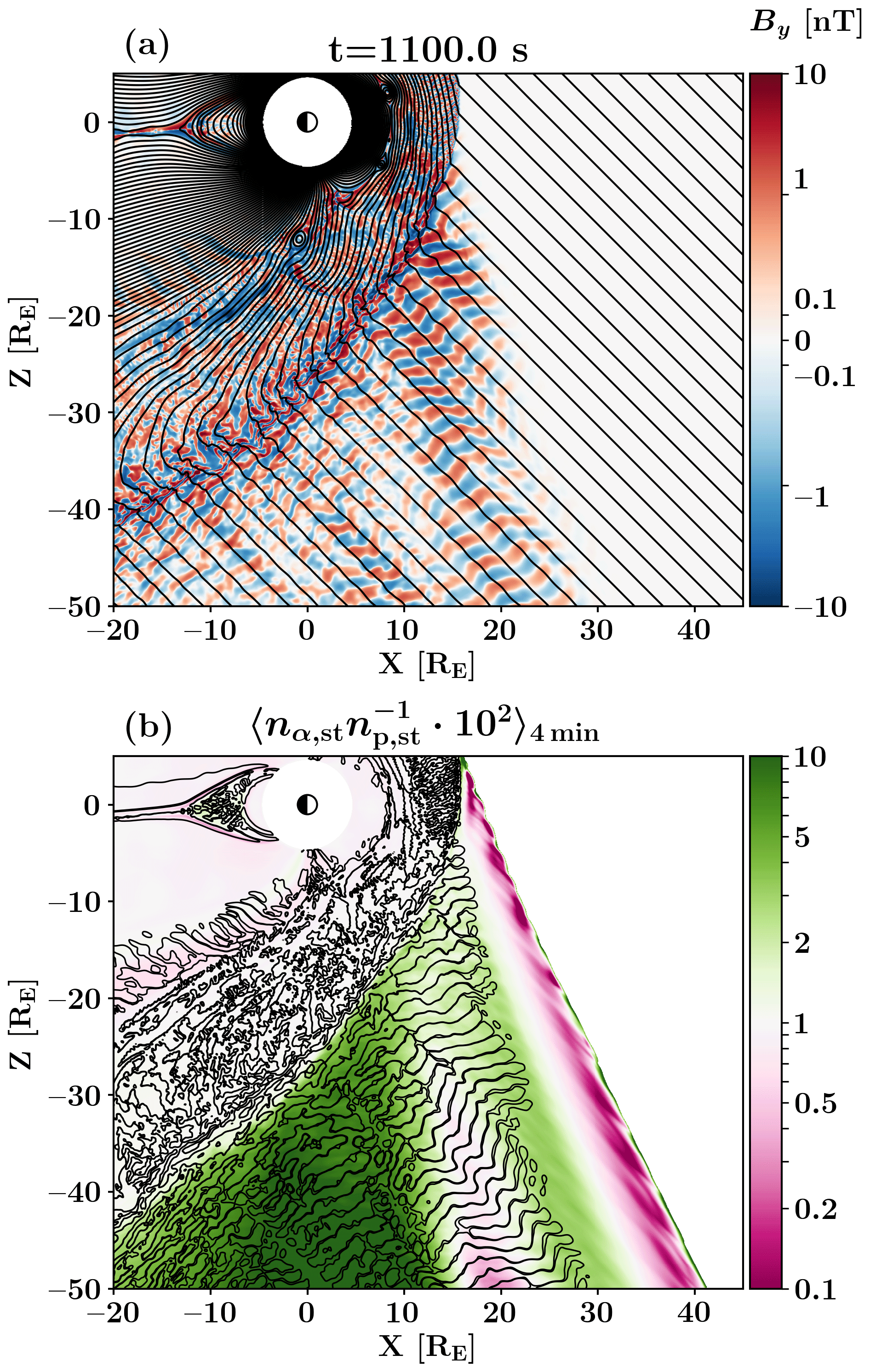
Figure 1Overview of the foreshock region of the simulation. (a) Out-of-plane magnetic field fluctuations By at 1100 s, using a symmetric logarithmic colour scale, indicating the extent of the ULF foreshock region. Black curves indicate magnetic field lines. (b) Ratio of suprathermal densities for helium over proton, normalized to the solar wind ratio of 1 %, averaged over a period of 4 min. The ratio is not shown in the pristine solar wind. Black contours are drawn for at time t=1100 s.
3.1 Foreshock edge
As shown in Fig. 1, the ion and ULF foreshocks are not identical in extent. The ULF foreshock edge visible in both panels connects to the bow shock at , whereas the ion foreshock edge intersects the bow shock already at (Fig. 1b). At the bottom of the figure, at , we see the ion foreshock extending up to X=40 RE, whereas the ULF foreshock only extends to a position ∼10 RE further downstream. We also see that, in Fig. 1b, the ratio of suprathermal alphas to protons in the foreshock shows significant deviations from the incoming solar wind ratio of 1 ∕ 100. Throughout most of the deep foreshock, the ratio, shown in Fig. 1b, tends to values ≳2, whereas at the foreshock edge, it falls below 0.2. This abundance of He2+ within the deep foreshock is likely a computational artefact, with H ions being efficiently scattered into the diffuse population, which is not tracked, whereas He2+ remains in non-gyrotropic partial rings and clumps. Right at the edge of the foreshock we see spatially periodic structures with, again, large alpha-to-proton ratios, likely caused by bursty reflection at the quasi-perpendicular shock and the alpha particles having larger gyroradii, thus gyrating further into the upstream. The ULF and ion dynamics of the foreshock edge are further examined in Fig. 2.

Figure 2(a) Magnetic field out-of-plane component By indicating the ULF foreshock extent. Contours indicate proton (black) and helium (green) suprathermal densities at 0.1 % (dotted contours) and 0.5 % (solid contours) of solar wind values. Four thick lines indicate the cut-throughs across the foreshock boundary. (b–e) Profiles across the foreshock at the positions shown in (a). Profiles are shown for suprathermal proton density (black solid line), suprathermal helium density (green solid line), and magnetic field magnitude (blue solid line). The horizontal dashed lines indicate 0.5 % (dashed line) of the solar wind density.
Figure 2a shows an excerpt from Fig. 1a, featuring a portion of the foreshock edge. The colour map is again the out-of-plane magnetic field component, overlaid with contours of proton (black) and helium (green) suprathermal densities. We focus on the contours upstream of the ULF foreshock. The solid contours are drawn where the suprathermal density is 0.5 % of the species' solar wind density and the dotted contours at 0.1 %, respectively. The thick grey lines indicate four cut-throughs across the foreshock edge. The magnetic field strength and the suprathermal proton and helium densities along these cuts are plotted in Fig. 2b–e. As shown in these plots, there is variation in the profiles of ions across the foreshock edge, moving into the foreshock from right to left. Close to the bow shock (Fig. 2b–c), there is a somewhat rapid increase in ion densities near 10 RE, followed by a gradual increase over the following 1–2 RE and finally plateauing values. Further out (Fig. 2d and e), we see a more gradual increase in suprathermal ion densities over several RE and a less clear plateau. The suprathermal ion density threshold at 0.5 % of the species solar wind density is shown as a horizontal dashed line.
We note that non-thermal particles are found several RE upstream of the foreshock waves, consistent with previous works showing that no ULF wave activity is observed in conjunction with the region closest to the foreshock edge where field-aligned beams are expected (and found). More importantly, we find significant amounts of suprathermal helium throughout the field-aligned beam region and into the ULF foreshock. As shown by the black and green contours in Fig. 2a, the helium foreshock edge is located equal to or slightly downstream of the proton foreshock edge. This shift is more pronounced in the dotted contours and increases when moving further away from the bow shock. At about 30 RE from the shock, the difference is of the order of 1 RE. The shift of the foreshock edge is also noticeable in the line profiles (Fig. 2b–e). This suggests that the proton foreshock is slightly more extended than the helium foreshock, and measurements made at the very edge of the foreshock can suggest significantly lower helium fractions despite the helium abundances rising to proton-comparable levels a few RE deeper within the foreshock. We also point out that the plateau of alpha particles inside the foreshock edge has more fluctuations to it than the plateau of protons.
We also note that the suprathermal ion density contours in Fig. 2 and the time-averaged ratios seen in Fig. 1 are not smooth, having a wavy shape instead. Supplementary Video A shows the wavy shape is due to intermittent reflection of ions at the bow shock, with bursts of ions propagating away from the shock along the field lines. This periodic and intermittent enhanced reflection of particles may be due to mesoscale reformation of the bow shock (Battarbee et al., 2020e) and can cause further discrepancies and variation in field-aligned beam densities.
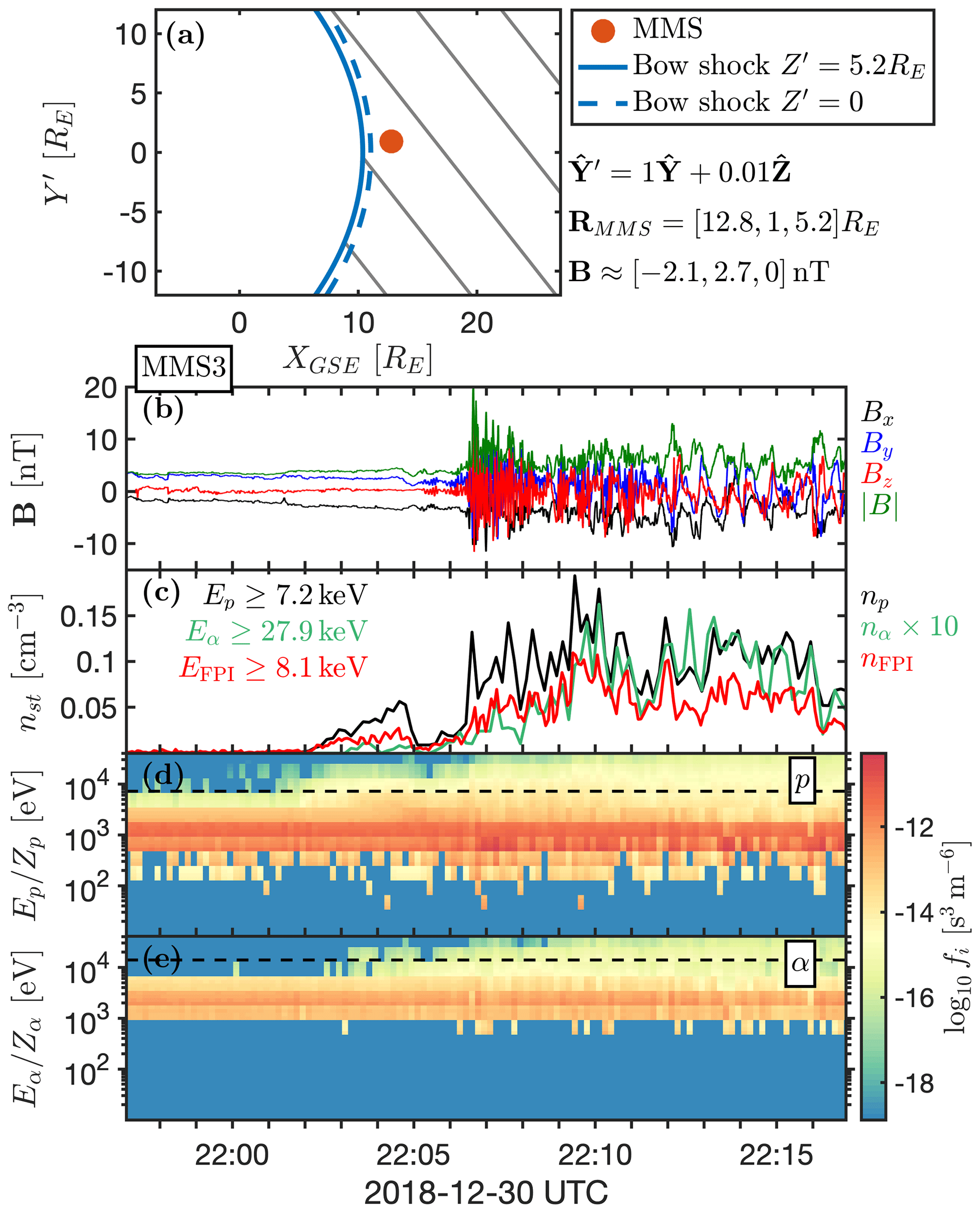
Figure 3MMS3 crossing from the solar wind into the foreshock region on 30 December 2018. (a) The MMS position relative to the bow shock just before the foreshock crossing in a plane that contains B. The solid blue line shows the bow shock position in the plane containing MMS and the dashed line in the plane containing Earth. The grey lines are the magnetic field lines. (b) The survey-mode measurements of the magnetic field magnitude and components, showing the spacecraft entering the ULF foreshock. (c) The number densities for H+ and He2+ suprathermal ions measured by HPCA with spacecraft frame energy cutoffs indicated in the legend, with the helium density multiplied by 10 to ease density evaluation. The FPI ion number density is shown for comparison. (d, e) The HPCA ion energy spectrograms for protons and helium, with the dashed line indicating the respective suprathermal ion cutoff energies.

Figure 4MMS3 crossing from the solar wind into the foreshock on 18 November 2018. The format is the same as in Fig. 3 but with He2+ multiplied by 25.
We now compare our numerical results with observations from the MMS spacecraft at the foreshock edge. Figures 3 and 4 show two time intervals during which the MMS3 spacecraft crossed from the solar wind into the foreshock region. Figures 3a and 4a show the spacecraft position relative to the bow shock model, which is scaled with the solar wind dynamic pressure (Farris et al., 1991; Schwartz, 1998). The plane is chosen so that B is in the plane and that Y′ is in the positive YGSE direction. Figures 3b–e and 4b–e, from top to bottom, show the IMF magnitude and components, the suprathermal densities of H+ (black; HPCA), He2+ (green; HPCA), and all ions (red; FPI) and proton and He2+ energy–time spectrograms from the HPCA instrument. The He2+ suprathermal densities have been multiplied by 10 or 25 to ease comparison of suprathermal ion density gradients. The lowest energy used in the calculation of the suprathermal (partial) densities for each species is also stated on the panel. This energy is about 4 times higher for alphas compared to the protons, due to larger mass of He2+. We note that the energy–time spectrograms show energy per charge , with the lowest energy included in the suprathermal population shown with the dashed line set to the values indicated in Figs. 3c and 4c. Also, only those suprathermal ions measured by HPCA (up to 40 keV∕e) are included in the densities, but we estimate the lost contribution due to higher energy ions to be small due to very small phase–space densities.
During both time intervals the transition between the foreshock and the undisturbed solar wind was not due to any IMF rotational discontinuity, as can be seen from the MMS magnetic field components. We also checked the solar wind measurements propagated to the bow shock nose from the OMNI database (King and Papitashvili, 2005) and found no sharp IMF change during those intervals. This means that the foreshock was undergoing gradual motion due to slow IMF rotations, so the spacecraft did not observe travelling foreshocks (Kajdič et al., 2017) or foreshock cavities (Schwartz et al., 2006; Billingham et al., 2008, 2011). This gradual motion of the foreshock region over the spacecraft location allows for magnetic field and suprathermal density profiles to be compared with those obtained from our simulations (Fig. 2).
Figures 3c and 4c show that the proton and He2+ suprathermal densities do not always behave in the same manner. In Fig. 3c, we can clearly see that the proton and He2+ suprathermal densities are well correlated across the foreshock edge, although H+ has a slightly stronger initial beam before 22:06 Coordinated Universal Time (UTC). Both increase with a similar relative gradient as the spacecraft crosses from the solar wind into the foreshock. In Fig. 4c, the suprathermal proton density starts to increase ∼3 min before the suprathermal He2+ density and remains low well into the foreshock. This suggests that the proton foreshock extends further outward than the He2+ foreshock. In other words, the proton foreshock extends to field lines connected to larger θBn values than the He2+ foreshock.
In order to better understand the different foreshock edge crossing behaviour seen in Figs. 3 and 4, we compare the main Vlasiator simulation used in this study to an equatorial plane simulation with a quasi-radial IMF, as detailed in Sect. 2.1. In Fig. 5, we show an enlarged view of the foreshock edge of both runs, with colour maps indicating the out-of-plane component of the magnetic field and black and green contours indicating proton and helium suprathermal densities at 0.5 % (solid) and 0.1 % (dotted) inflow densities, averaged over 2 min. In comparing the Vlasiator plots with MMS observations, it is important to keep in mind that the Vlasiator definition for suprathermals includes reflected particles with simulation frame energies comparable with the solar wind bulk, whereas the MMS suprathermal density is defined with a markedly higher minimum energy threshold. Comparison of Fig. 5a–b indicates that simulations can reproduce the two different foreshock edge behaviours, with Fig. 5a (our main run) presenting a relatively rapid drop-off and Fig. 5b (the quasi-radial IMF comparison run) showing a much more gradual fall-off of suprathermal ion densities and a greater difference between the two ion species.
The IMF prior to the 30 December 2018 foreshock edge crossing had the IMF pointing in the dawn, anti-sunward direction with its cone angle . Consequently, this was also the orientation of the foreshock. At the time, MMS3 was located near the nose of the Sun–Earth line, at approximately in GSE coordinates. This location, together with large IMF cone angle, means that the foreshock edge was crossed in a way that is qualitatively similar to that shown in Fig. 5a.
In the case of the 18 November 2018 event, the IMF cone angle was and pointing in the northern, anti-sunward direction prior to the foreshock encounter, and consequently, this was also the foreshock orientation. The GSE coordinates of MMS3 were , i.e. far from the Sun–Earth line. Thus, this foreshock edge crossing is comparable with the one shown in Fig. 5b.

Figure 5An enlarged view of the foreshock edge, with the magnetic field out-of-plane component Boop indicating the ULF foreshock extent. Contours indicate suprathermal ion densities, as in Fig. 2a, but averaged over 2 min. (a) The meridional plane 45∘ IMF simulation used in the majority of this paper. (b) An equatorial plane 5∘ IMF run for comparison. The IMF orientation appears to affect the suprathermal ion density gradient at the foreshock edge.
3.2 Velocity distribution functions and their properties
We now examine the properties of ion velocity distribution functions (VDFs) at the edge of and within the foreshock. Figure 6 shows 2D projections of proton and helium velocity distribution functions in the solar wind frame at three positions close to the foreshock edge, extracted from our Vlasiator simulation at time 1000 s. In Fig. 6 (panels 1–2 and 4, subpanels ), we show projections that have been generated by averaging the instantaneous VDFs over the vB×V direction, whereas subpanels labelled have been averaged over the vB direction. We use two different colour scales to differentiate the phase–space densities of the two ion species, with ranges selected to account for the input solar wind abundance ratio. Figure 6 (panels 1–2 and 4) shows VDFs from virtual spacecraft locations (A, B, and C, respectively). The Fig. 6 subpanels also show an ellipsoid located at the position in velocity space where particles would end up if they were specularly reflected from the solar wind population at the closest point of the bow shock. The shock location was determined according to a plasma compression criterion of np>2np,sw, and the shock normal direction was estimated to be equal to a vector pointing from the closest shock location to the virtual spacecraft location. We emphasize that this estimate is a rough one, to be improved upon in future studies, and does not account for ion propagation times, drifts, or the existence of an electron pressure gradient cross-shock potential. Figure 6 (panel 3) shows an overview of the foreshock region, indicating the locations of the spacecraft on top of a colour map depicting the temperature anisotropy calculated from the whole proton VDF. The dark orange region at the upstream edge of the foreshock, with parallel temperatures in excess of perpendicular temperatures, is indicative of the FAB region of the proton foreshock. Magnetic fields lines are depicted with black curves.
In panel 1 of Fig. 6, at the position of virtual spacecraft A located very close to the foreshock edge, we see very clear proton and helium FABs, though the helium beam appears to have more structure. Parallel velocities of both beams are between 1500 and 2000 km s−1 in the solar wind frame or in the simulation frame, which translates to roughly 3–5 keV nuc−1. We note that this is larger than the energy at which specularly reflected particles would be found, which suggests that these particles have experienced shock drift acceleration (SDA) at the quasi-perpendicular shock front. This indicates that the source of the FABs in panel 3 of Fig. 6 is located at roughly . Panel 2 of Fig. 6 depicts VDFs at position B, at the boundary between the FAB region and the ULF foreshock. At this location, the ion beam seems to be transitioning into a more gyrating distribution, with a gyrophase-bunched signature (visible in the panel at ) for both species but particularly for helium at . Parallel velocities have begun to decrease, extending down to 1000 km s−1 in the solar wind frame of reference. A similar upstream ion velocity decrease was also seen in Battarbee et al. (2020e). Still, at this position, both helium and protons show a qualitatively similar shape to their distribution functions. Conversely, in panel 4 of Fig. 6, at position C, the proton VDF resembles a low-energy field-aligned beam, extending from 1000 to 1800 km s−1 in vB, whereas the helium distribution has very little trace of a beam, instead consisting of a broken up gyrating ion population. An animated version of Fig. 6 can be found as Supplementary Video B. We also note that, early in this video, at virtual spacecraft A, the helium VDF in particular shows what appears to be a gyrophase-bunched population but which remains stationary in velocity space. We deduct that it is in fact spatial sampling of the helium foreshock edge, visible due to the large gyroradius of alpha particles. We also point out that the proton beam energy found, in particular, in panel 1 of Fig. 6 does not extend to the tens of keV∕e found in some spacecraft observations, possibly a result of the sparse velocity space implementation in Vlasiator.
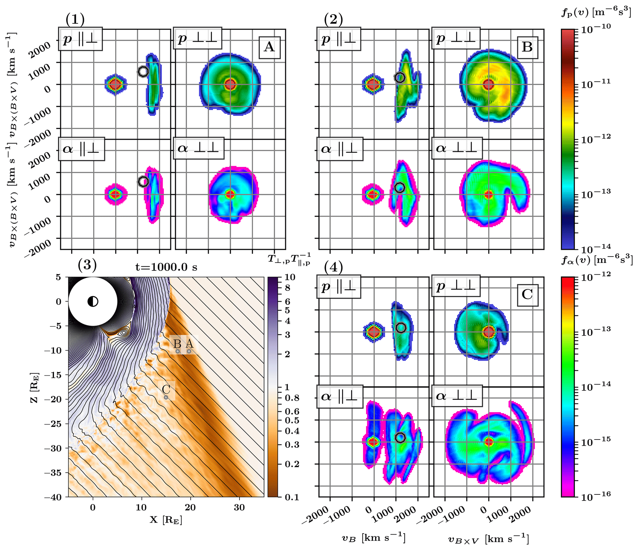
Figure 6Velocity distribution functions (VDFs) for protons and alpha particles and their locations in the foreshock. (3) Map of the foreshock, with three VDF positions indicated with capital letters. The colour indicates the proton temperature anisotropy, with magnetic field lines in black. Panels (1), (2), and (4) show sets of four projections of ion VDFs at virtual spacecraft locations in the solar wind frame. Coordinates are chosen to represent two positions at the foreshock boundary (A and B) and one just within the ULF foreshock (C). In each set, the subpanels are labelled as vB versus (; left columns) or vB×V versus (; right columns) and protons (top rows) or helium (bottom rows). The black and white circles estimate the areas of specular reflection.
Figure 7 is similar to Fig. 6 but with virtual spacecraft locations chosen to represent regions further within the foreshock and also closer to the quasi-parallel bow shock. Panels 1 and 2 of Fig. 7 show spacecraft D and E, which are located close to the bow shock and depict mostly gyrating and intermediate ion populations. The helium populations of gyrating ions appear to have more structure to them. It is also noteworthy that both proton and helium subpanels of panel 1 in Fig. 7 have what looks like a FAB propagating towards the shock at a parallel velocity greater than the solar wind speed, with velocities vB<0. Although the estimate of the velocity space location of specularly reflected particles does not account for particle travel times or shock shape evolution, we find that the near-circular ellipsoids indicating potential specular reflection are usually found in VDF regions where there are enhancements, suggesting that specular reflection indeed plays a role in the generation of these populations. As the bow shock reforms as a mesoscale process with distinctly non-planar features, the direction of specular reflection varies, leading to the intermittent and gyrating partial rings seen in these VDFs. This mapping of specular reflection can also be seen in Supplementary Video C, which is an animated version of Fig. 7. Panel 4 of Fig. 7 shows proton and helium VDFs further within the deep foreshock and away from the bow shock. The proton population appears to be a gyrating ion population, and the helium population is a low-energy beam population, but viewing the VDFs at different times (see Supplementary Video C) shows that both ions usually resemble gyrating ion populations.
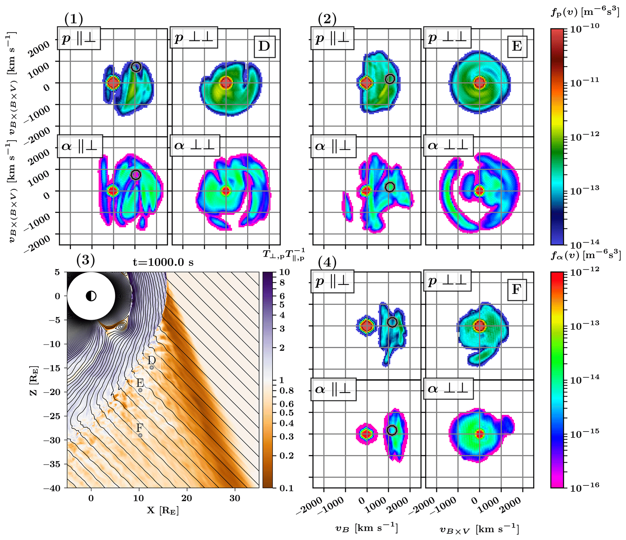
Figure 7Velocity distribution functions for protons and alpha particles and their locations in the foreshock. (3) Map of the foreshock with three VDF positions indicated with capital letters. The colour indicates proton temperature anisotropy, with magnetic field lines in black. Panels (1), (2), and (4) show sets of four projections of ion VDFs at virtual spacecraft locations in the solar wind frame. Coordinates are chosen to represent two positions close to the quasi-parallel bow shock (D and E) and one deep within the outer foreshock (F). In each set, subpanels are labelled as vB versus (; left columns) or vB×V versus (; right columns) and protons (top rows) or helium (bottom rows). The black and white circles estimate the areas of specular reflection.
In light of the complex simulated VDF shapes, and in order to obtain a better understanding of global foreshock ion characteristics, we show, in Fig. 8, plots of global per-species temperature anisotropies and a measure of per-species non-gyrotropy. We apply the temperature anisotropy to the whole VDF, allowing us to identify regions where VDFs have FAB-like features showing up as anisotropy values much smaller than 1. The agyrotropy measure (Swisdak, 2016) is as follows:
where is the parallel pressure, is the perpendicular pressure, and P12, P13, and P23 are off-diagonal pressure tensor components that can be used to evaluate the complexity of the VDF and the role of gyrating ions. For a completely gyrotropic distribution, Qag=0 and Qag=1 would signify a maximal deviation from gyrotropy. Figure 8a–b show agyrotropies for protons and helium, respectively, and Fig. 8c–d show temperature anisotropies. The panels in Fig. 8 also show out-of-plane magnetic field contours at a level of ±0.2 nT, indicating the extent and structure of the ULF foreshock. We find that the FAB region of protons is clearly visible in Fig. 8c at the edge of the ion foreshock as a dark orange band (). In Fig. 8a we see the same structure at the foreshock edge. It is visible as a band of medium green blobs (Qag,p∼0.01) close to the shock nose, transitioning to paler green thin streaks (Qag,p∼0.001) away from the shock.
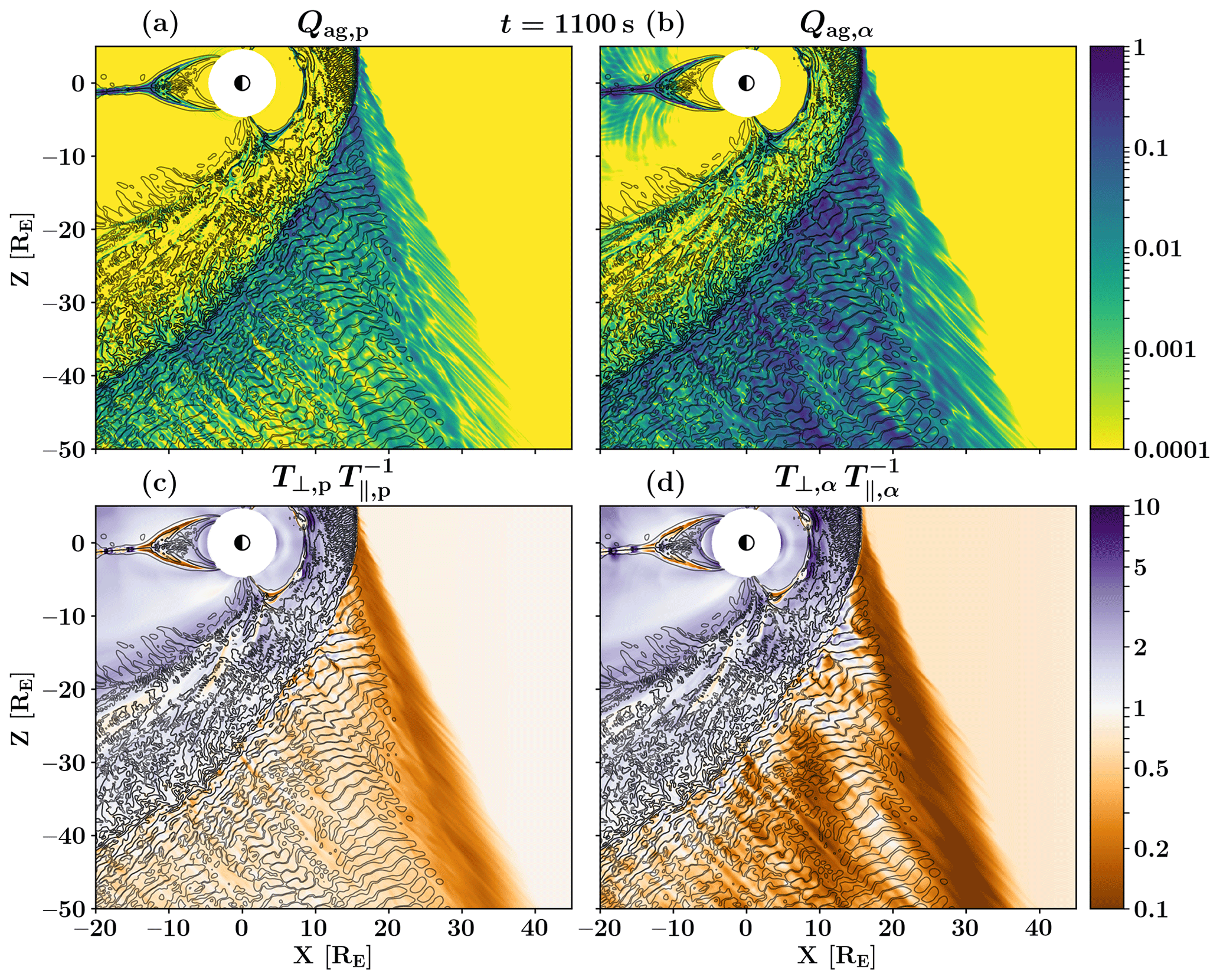
Figure 8Foreshock characteristics for proton and helium at 1100 s. (a, c) Protons and (b, d) helium are shown. (a, b) Agyrotropy Qag (see Eq. 1), where a value of 0 corresponds with perfect gyrotropy. (c, d) Temperature anisotropy calculated for the total distribution function, including both solar wind and suprathermal parts. Black contours show the out-of-plane magnetic field By fluctuations at a level of ±0.2 nT, indicating the extent of the ULF foreshock region.
For helium, in Fig. 8d, this FAB region at the edge of the foreshock is also clearly visible, with very low anisotropy values. Interestingly, helium also shows a parallel pressure signature (dark orange low anisotropy values) deeper in the foreshock. This region coincides with a weakening of the ULF foreshock, visible in the destructuring of wave fronts (black contours) in the vicinity of (). Referring to Fig. 1b, we see that this band of low-energy, FAB-type alpha particles coincides with an increase in the measured helium fraction, which continues downstream from that point.
Figure 8a–b show, in particular for protons, an enhancement in agyrotropy at the boundary between the FAB region and the ULF foreshock. This dark green region is a signature of gyrating and gyrophase-bunched ions at this boundary, in agreement with Meziane et al. (2004), Mazelle et al. (2007), and Andrés et al. (2015). This effect can also be seen at virtual spacecraft location B in Fig. 6 (panel 2; () and () subpanels), as a gyrophase-bunched extension of the ion distribution. We note that this increase in agyrotropy and, thus, gyrating ions matches the ULF foreshock and previous studies well, down to about , but the boundary becomes less well defined further out, away from the shock. We also note that Fig. 8b shows darkened bands of increased agyrotropy on both the upstream and downstream edges of the inner-foreshock-heightened parallel pressure alpha particle band, which suggests there might be similar gyrophase sampling taking place as for the foreshock FAB beam proper.
For both protons and helium, we see striped enhancements of agyrotropy right at the outer ion foreshock boundary, indicative of spatial sampling of gyrating ion beams right at the outermost foreshock edge. The gyration of these ion beams, accelerated at the quasi-perpendicular shock front and made non-uniform by the rippling of the shock front, is particularly visible in Supplementary Video D, which is an animated version of Fig. 8. Finally, we note that large regions of the foreshock close to the quasi-parallel bow shock show signatures of temperature anisotropies ≳1 and enhanced agyrotropies, which are likely a signature of specular reflection of ions at the quasi-parallel bow shock.
3.3 Foreshock waves
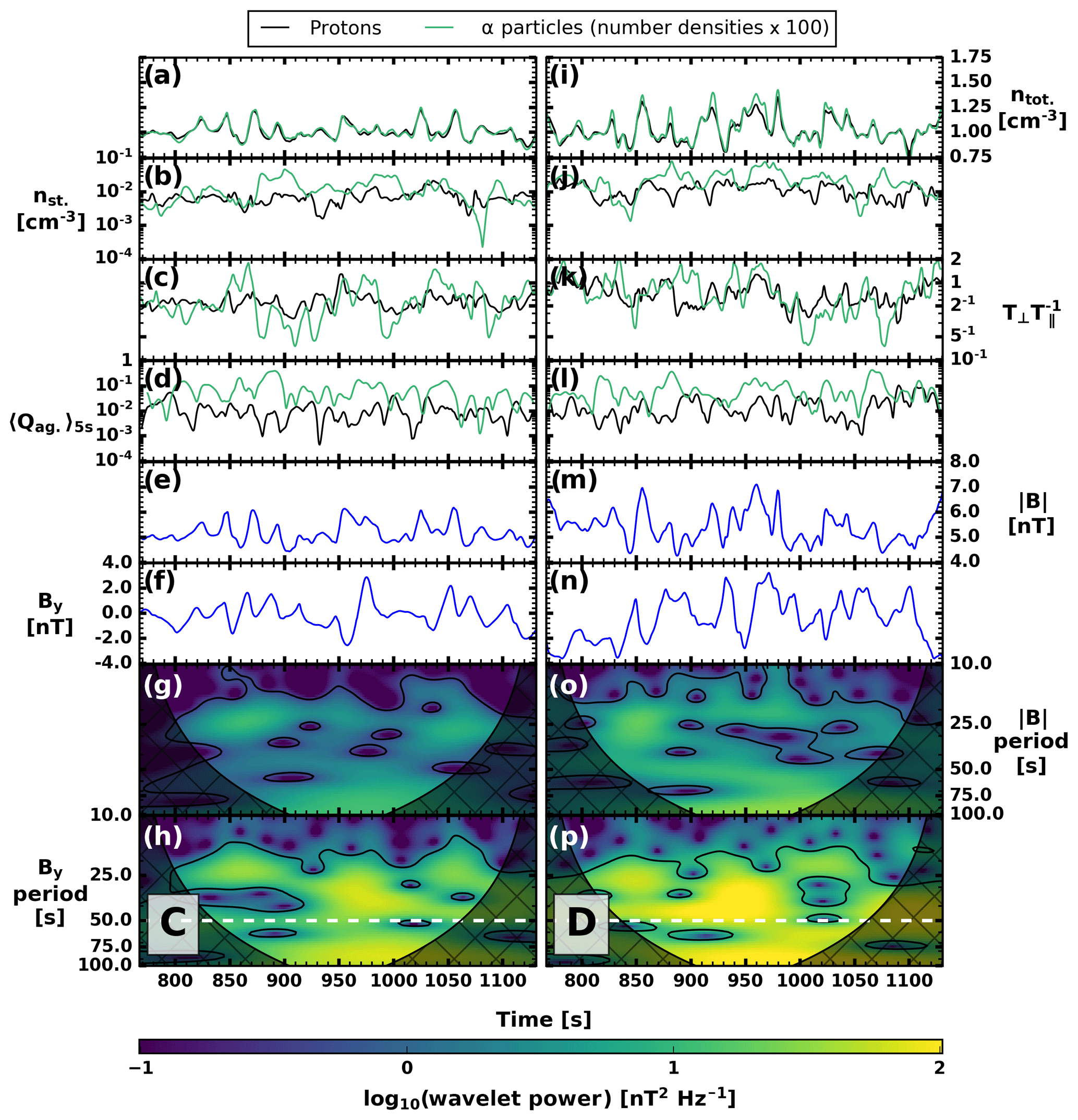
Figure 9Time series and wavelets at virtual spacecraft positions C (a–h) and D (i–p) at the edge of the ULF foreshock. Panels (a–d) and (i–l) show proton (helium) quantities in black (green). (a, i) Total number densities. (b, j) Suprathermal number densities on a logarithmic scale. (a, b, i, and j) The helium number densities have been multiplied by 100. (c, k) Temperature anisotropies. (d, l) Agyrotropy Qag measured as a 5 s running average. (e, m) Magnetic field magnitudes . (f, n) Magnetic field out-of-plane components By. (g, o) Wavelet power spectra of fluctuations. (h, p) Wavelet power spectra of By fluctuations. The black contours show the 95 % confidence level, and the cross-hatched regions denote the cone of influence. The white dashed lines show the expected frequency of By fluctuations (see text).
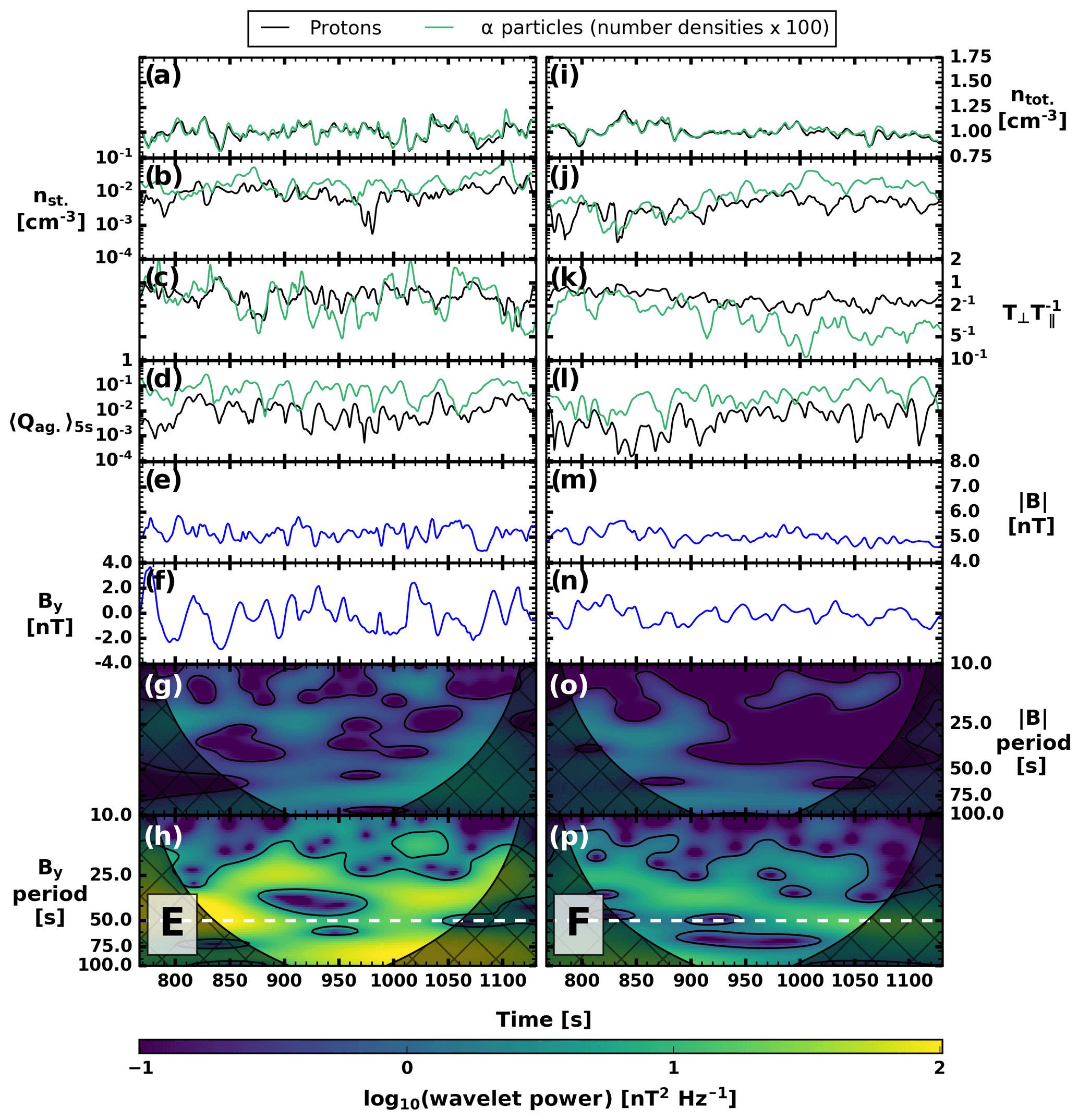
Figure 10Time series and wavelets at virtual spacecraft positions E (a–h) and F (i–p) in the ULF foreshock. Panels (a–d) and (i–l) show proton (helium) quantities in black (green). (a, i) Total number densities. (b, j) Suprathermal number densities on a logarithmic scale. (a, b, i, and j) The helium number densities have been multiplied by 100. (c, k) Temperature anisotropies. (d, l) Agyrotropy Qag measured as a 5 s running average. (e, m) Magnetic field magnitudes . (f, n) Magnetic field out-of-plane components By. (g, o) Wavelet power spectra of fluctuations. (h, p) Wavelet power spectra of By fluctuations. The black contours show the 95 % confidence level, and the cross-hatched regions denote the cone of influence. The white dashed lines show the expected frequency of By fluctuations (see text).
Figures 9 and 10 show measurements from virtual spacecraft placed at locations C, D, E, and F in the foreshock (see Figs. 6 and 7). The top row in each plot displays the total number density ntot for protons and helium, and the second row displays their suprathermal number densities nst. In both rows, the helium number densities have been multiplied by a factor of 100 to ease the comparison with proton number densities. Note that the suprathermal number densities are shown on a logarithmic scale, since the values vary significantly. In the third row, temperature anisotropy is displayed, and the fourth row displays the agyrotropy measure Qag. The time series of Qag have been smoothed out with a 5 s running average to help readability due to a large number of high-frequency fluctuations. The fifth and sixth rows display the total magnetic field and its out-of-plane component By, respectively.
The fluctuations of H+ and He2+ total densities follow each other quite closely at all locations, though the amplitude of the He2+ density oscillations is larger than that of protons at point D and E. These larger He2+ density variations seem to be well correlated with the fluctuations of the He2+ suprathermal density at position D (Fig. 9j) but not so much at point E (Fig. 10b). At all locations analysed with these virtual spacecrafts, the suprathermal ion ratio is larger than the solar wind ion ratio , as shown already by Fig. 1b. The agyrotropy is also more pronounced for He2+ than for H+, as illustrated in Fig. 8a–b, and with the VDF discussed in the previous section.
The two bottom rows of Figs. 9 and 10 (panels g, h, o and p) display the wavelet power spectra of and By, in order to investigate foreshock wave activity. The wavelet transform (Torrence and Compo, 1998) is calculated using the Morlet wavelet. The black contours in the power spectra show the 95 % confidence level, and the cross-hatched regions bordering the spectra depict the cone of influence, where edge effects arising due to the time series' endpoints become important. The horizontal dashed line on the By wavelet power spectra is drawn at 50 s, which is close to the expected spacecraft frame period of foreshock fast magnetosonic waves for these upstream conditions, according to empirical models (Le and Russell, 1996; Takahashi et al., 1984). At all four positions, an enhancement in the By component power spectra can be seen in the vicinity of this period, which is in agreement with previous works showing that fast magnetosonic waves permeate the foreshock in Vlasiator simulations as in spacecraft observations (Palmroth et al., 2015; Turc et al., 2018). We note that none of the virtual spacecraft selected here display the typical quasi-monochromatic foreshock waves shown in these previous studies, due to their relative proximity to the bow shock (≲7 RE). In the vicinity of the shock, the wave activity is more complex due to nuanced interactions between the waves and the diffuse ion population (Greenstadt et al., 1995; Turc et al., 2018).
At point F we find weaker wave activity, despite its location deep within the foreshock. This is most likely due to the low density of suprathermal gyrating or beam particles in this part of the foreshock (see Fig. 10j). This results in a lower wave growth rate as this parameter depends on the beam density for the beam–beam instabilities at play in the foreshock (Gary, 1993). This weaker wave activity is accompanied by a lower temperature anisotropy for the He2+ ions, due to the suprathermal He2+ population being in the form of low-energy, field-aligned beams in this region (see Fig. 7, panel 4). Comparing the positions of our virtual spacecraft with Fig. 8 and the contours indicating well-structured or more broken up ULF wave fronts, we see that the weakest wave power (point F) is seen at the most broken up position, and the strongest power (point D) is found at a position of well-structured wave fronts.
According to previous works, the plasma rest frame frequency of foreshock fast magnetosonic waves generated by proton beams is of the order of 10 % of the proton gyrofrequency, probably due to the cyclotron resonance which gives rise to the waves (Hoppe and Russell, 1982; Eastwood et al., 2005; Wilson, 2016). He2+ ions have a gyrofrequency that is half that of protons. He2+ ion beams could, thus, generate fast magnetosonic waves at a period of ∼100 s with the upstream parameters used in our simulation. The wavelet power spectra in Figs. 9 and 10 show enhanced wave power around ∼100 s, but this part of the spectra is mostly inside the cone of influence of the wavelet transform, making it difficult to draw firm conclusions. Moreover, the analysis of the foreshock wave properties in an identical Vlasiator run without a helium population (not shown) reveals similar enhancements of the wave power at ∼100 s. It is therefore unlikely that these fluctuations are due to helium beam instabilities. Thus, despite a 1 % solar wind helium content providing non-negligible mass loading, we find the helium component to not have a significant impact on foreshock wave populations.
In this study, we present how sometimes the proton foreshock extends further out upstream than the helium foreshock. Our model of the edge of the foreshock shows that, within a few RE of the foreshock edge, the ratio of suprathermal alphas to protons (as shown in Fig. 1b) often tends towards a value of about 10 times less than the solar wind. This seems to be in excellent agreement with Fig. 1b of Fuselier and Thomsen (1992). They restricted the analysis of beam ions to high energies (1.6–5.7 times the solar wind energy), which will likely require measurements very close to the foreshock edge. At any given distance from the shock, slower particles will have travelled for a greater period of time and will thus have drifted deeper into the foreshock due to, for example, E×B drift. In the central section of the FAB region, but still outside the ULF foreshock, we report a suprathermal alpha fraction of the order of the solar wind value. At the very sunward edge of the foreshock in Fig. 1b, some regions of relatively more abundant suprathermal alphas can be seen, and we suggest that this is an effect stemming from the larger gyroradii of alpha particles, as the feature is clearly spatially periodic.
In our simulation, we find that, well inside of the upstream edge of the foreshock, there is a region with strong, well-structured ULF wavefronts and a relative decrease in suprathermal alpha particles, as shown in Fig. 1b. We suggest that this could be due to these very strong proton-driven ULF waves being strong enough to scatter even alpha particles which are not in resonance with the wave oscillation, due to a larger mass-to-charge ratio than that of protons. Further inside the foreshock, the ULF wave front breaks up into less uniform waves. This break-up is inherent to proton dynamics and not caused by the presence of alphas. Previously, the growth of waves with distance from the foreshock edge has been reported in Le and Russell (1992), but their study was performed close to the nose of the shock, whereas the destructuring we report takes place far along the flank of the bow shock. In this region we report a helium fraction higher than that of the solar wind. One possible explanation for this is that the destructured ULF waves are still able to scatter protons, but alpha particles propagate in a less disturbed fashion, more akin to a low-energy FAB. This is seen as a second region of parallel pressure enhancement for alphas in Fig. 8d.
Based on the time–energy spectrogram results in panels d and e of Figs. 3 and 4, it appears that the foreshock edge transitions for H+ and He2+ were in more agreement for the December 2018 event than for the November 2018 event. During the event depicted in Fig. 3, the IMF upstream of the foreshock was dominated by the By component, and MMS was located at approximately and Z=5RE (roughly at the nose of the shock). If we assume a parabolic bow shock shape, the field lines at the foreshock edge were thus connected to a region of the shock where . For each field line, we can estimate the derivative of θBn as follows:
where is a normalized spatial distance vector perpendicular to the foreshock edge. At the location of MMS with the listed IMF conditions, the derivative of θBn respective to the distance to the foreshock edge is large. Conversely, during the event depicted in Fig. 4, MMS was located at approximately and Z=6RE, i.e. somewhat at the flank, and the IMF had a strong −Bx component. Thus, the field lines at the foreshock edge can be assumed to connect to a region where the corresponding derivative of θBn for each field line is small. When comparing two Vlasiator simulations with different IMF directions in Fig. 5 and corresponding qualitatively with the MMS observation situations, we see qualitatively similar behaviour. We note that the contours in Fig. 5 were averaged over time, smoothing out variations due to ion gyroradii, ion gyrotimes, and reflection variations due to mesoscale bow shock reformation. Variations such as these are detectable in virtual and real spacecraft measurements. Based on this comparison, we suggest that the different profiles of the foreshock edge transition, seen particularly well in the suprathermal ion densities, may be related to the derivative of θBn for the connecting field line, as we are able to replicate the MMS observation variation in the gradient of suprathermal ion profiles using two simulation runs with different IMF cone angles. In a previous study, Sibeck et al. (2008) investigated foreshock edge gradients in radial IMF hybrid simulations, finding a correlation with model dipole tilt. They stated that their bow shock edges were still propagating outwards, and the foreshock in their Fig. 1 appears tilted to the south, possibly as a result of non-radial magnetic field components and, perhaps, a similar underlying cause as in our explanation. This can be investigated further in both observational and simulational studies.
Figure 8 shows that helium exhibits a greater agyrotropy throughout the ion foreshock. Interestingly, enhanced helium agyrotropy appears to coincide with well-structured ULF regions. This suggests that the mostly proton-induced ULF waves might be efficient drivers of agyrotropy for gyrating He2+ ions which have half the gyrofrequency of protons, leading them to scatter into the diffuse distribution. Proton-induced waves have been shown to heat the solar wind helium populations (Hollweg and Turner, 1978; Dusenbery and Hollweg, 1981). We propose that this additional heating by ULF waves is one reason for the helium ions exhibiting greater agyrotropy values than protons throughout the foreshock. Another source of agyrotropy and VDF break-up in helium may be that He2+ ions have greater gyroradii than H+ ions, and thus, each ion scans a greater extent of foreshock waves and structures.
We note the absence of a diffuse population of ions in our proton and helium VDFs in Figs. 6 and 7 but deduce that it is due to the low phase–space density of the diffuse ion population extending below our velocity space sparsity threshold, leading to those ions being discarded. We do not expect the diffuse ion population to strongly affect the wave dynamics, maintaining reasonable validity of the rest of our results. We do admit that some of our deductions about proton and alpha particle scatterings depend on this assumption that the suprathermal density decrease can be interpreted as the scattering of ions from a gyrating population to a diffuse population. At least some of the reported relative alpha particle abundance in Fig. 1 can be attributed to this, which agrees with the proton-induced ULF waves being more efficient at scattering protons, leading to a greater portion of the proton suprathermal population scattering into the diffuse part of velocity space, whereas alphas remain as gyrating ions tracked by the simulation (and resulting in high agyrotropies as well). We also note that our study is limited to lower energy FABs with energies of the order of 1–1.5 times the solar wind energy. The lack of a deka–keV FAB in our simulation may result from our choice of cold electrons, i.e. no electron pressure gradient term at the shock front. Since protons with a mass-to-charge ratio of 1 would feel the effect of a cross-shock potential stronger than alpha particles would, this can also partially explain the predominantly large helium fraction in our simulated foreshock.
We evaluate virtual spacecraft wavelets, looking for signatures of waves driven by helium beam instabilities, which could develop together with the proton beam instabilities in the foreshock, but we do not find convincing evidence for such waves. This result is as expected because of the low abundance of He2+ ions in our simulation, i.e. only 1 % of the solar wind proton number density. This number density is still enough to cause mass loading, pushing the bow shock 0.5–1.0 RE further towards the Earth than in a comparative run without helium (comparison not shown here; for the other simulation see Blanco-Cano et al., 2018). Future simulations with a higher helium-to-proton ratio will allow further investigation of helium-driven waves in the foreshock. We note that, due to the ratio of gyrofrequencies, simulations must be run for an extended period of time in order to accurately capture potential helium-induced waves.
Providing a point of comparison with a similar model, Jarvinen et al. (2019) simulated the magnetosphere and the foreshock of Mercury with a global hybrid cloud-in-cell model, including 4 % of He2+ ions in solar wind. Jarvinen et al. (2019) presented a fast-mode ULF wave field at wave periods of approximately 5 s, and populations of both H+ and He2+ were present in the quasi-parallel bow shock region, with He2+ backscattering found to be more efficient than for H+. Similar to our model, they did not include an electron pressure gradient term. We note that, despite how the Hermean magnetosphere is much smaller and the impinging solar wind is quite different from that at the Earth, some properties of ULF waves at different planetary foreshocks appear to scale with respect to the interplanetary magnetic field magnitude, as illustrated by Hoppe and Russell (1982). Additionally, Fig. 1b shows proportionally enhanced suprathermal He2+ densities compared to H+, which is similar to the point result in Jarvinen et al. (2019), but we also show spatial structure in the ratio of the suprathermal populations.
In summary, we show how, for the simulated solar wind conditions, He2+ is a significant foreshock species which has dynamics similar to those of protons but with distinct properties, such as preferential heating by proton-induced ULF waves. Both protons and helium are found in the FAB at the foreshock edge, with beam energies decreasing from ≳ 5 to when going from the foreshock edge to the inner edge of the FAB region. Helium ions are found to exhibit more agyrotropy than protons, probably due to their interaction with the proton-dominated ULF waves.
The profiles of suprathermal abundances of proton and helium at the foreshock edge show variability, both in Vlasiator simulations and in MMS data, and we show how this may be explained with the prevailing IMF orientation affecting the derivative of θBn at the field-line-connected position at the bow shock.
Vlasiator (https://www.helsinki.fi/en/researchgroups/vlasiator; Palmroth, 2020) is distributed under the GPL-2 open source license at https://github.com/fmihpc/vlasiator/, https://doi.org/10.5281/zenodo.3640593 (Palmroth and the Vlasiator team, 2020). Vlasiator uses a data structure developed in-house at the University of Helsinki, and it is available at (https://github.com/fmihpc/vlsv/, Sandroos, 2019). The Analysator software is available at (https://github.com/fmihpc/analysator/; Hannuksela and the Vlasiator team, 2020) and was used to produce the presented figures. The run described here takes several terabytes of disk space and is kept in storage maintained within the CSC – IT Center for Science. Data presented in this paper can be accessed by following the data policy on the Vlasiator website.
The supplementary videos A, B, C, and D provide movie extensions of Figs. 1b, 6, 7, and 8, showcasing the temporal evolution of foreshock features and particle population shapes and properties. Movie A (Battarbee, 2020a) is a filmed extension of Fig. 1b. The animation of the foreshock region of the simulation includes over 250 s of simulation. The ratio of suprathermal densities for helium over protons is normalized to the solar wind ratio of 1 %. The ratio is not shown in the pristine solar wind. Black contours are drawn for . Movie B (Battarbee, 2020b) is a filmed extension of Fig. 6. It shows the animation of velocity distribution functions for protons and alpha particles and their locations in the foreshock. Panel 3 shows a map of the foreshock, with three VDF positions indicated with capital letters. The colour indicates the proton temperature anisotropy, with magnetic field lines in black. Panels 1, 2, and 4 show sets of four projections of ion VDFs at virtual spacecraft locations in the solar wind frame. Coordinates are chosen to represent two positions at the foreshock boundary (namely A and B) and one just within the ULF foreshock (C). In each set, the subpanels are labelled as vB versus (; left columns) or vB×V versus (; right columns) and protons (top rows) or helium (bottom rows). Movie C (Battarbee, 2020c) is a filmed extension of Fig. 7. It shows an animation of the velocity distribution functions for protons and alpha particles and their locations in the foreshock. Panel 3 shows a map of the foreshock, with three VDF positions indicated with capital letters. The colour indicates the proton temperature anisotropy, with magnetic field lines in black. Panels 1, 2, and 4 show sets of four projections of ion VDFs at virtual spacecraft locations in the solar wind frame. Coordinates are chosen to represent two positions close to the quasi-parallel bow shock (D and E) and one deep within the outer foreshock (F). In each set, subpanels are labelled as vB versus (; left columns) or vB×V versus (; right columns) and protons (top rows) or helium (bottom rows). Movie D (Battarbee, 2020d) is a filmed extension of Fig. 8. It shows an animation of the foreshock characteristics for proton and helium over 363 s of simulation. The left column (panels a and c) shows protons, and the right column (panels b and d) shows helium. The top row shows agyrotropy Qag (see Eq. 1), where a value of 0 corresponds with perfect gyrotropy. The bottom row shows temperature anisotropy , calculated for the total distribution function including both solar wind and suprathermal parts. Black contours show the out-of-plane magnetic field By fluctuations at a level of ±0.2 nT, indicating the extent of the ULF foreshock region.
This paper was outlined and drafted at the Third International Vlasiator Science Hackathon held in Helsinki, Finland, on 19–23 August 2019. MB, XBC, LT, and PK performed the preliminary investigation leading to the team effort. MB led the investigation and the writing process. AJ provided the MMS plots and SF and KT verified them. VT performed the wavelet analysis with the help of LT. MP led the Vlasiator team and organized the hackathon. UG and YPK were instrumental in adding helium support to Vlasiator. All coauthors (including MA, TB, MAT, TK, SR, MD, and JS) provided scientific input during the Hackathon event, during the pre-submission review process, or both.
The authors declare that they have no conflict of interest.
This paper was outlined and drafted at the Third International Vlasiator Science Hackathon held in Helsinki, Finland, on 19–23 August 2019. The hackathon was funded by the European Research Council (grant no. 682068) under the PRESTISSIMO project. We acknowledge the European Research Council for the Starting grant (grant no. 200141-QuESpace), with which Vlasiator was developed, and the Consolidator grant (grant no. 682068-PRESTISSIMO), awarded to enable the further development of Vlasiator for scientific investigation. The Finnish Centre of Excellence in Research of Sustainable Space, funded through the Academy of Finland (grant no. 312351), also supported the Vlasiator development and science. We also gratefully acknowledge the Academy of Finland (grant nos. 322544, 328893, and 309937). XBC acknowledges support from the UNAM PAPIIT-DGAPA project (grant no. IN105218-3) and CONACyT (grant no. 255203). MAT acknowledges support from NASA MMS (grant no. NG04EB99C), NASA MMS GI (grant no. 80NSSC18K1363), NASA (grant no. 80NSSC18K0999), and the DGA project at École Polytechnique (grant no. 2778/IMES). Primož Kajdič's work has been supported by PAPIIT (grant no. IA101118). Research at the Southwest Research Institute, Texas, USA, was supported by the MMS prime contract (grant no. NNG04EB99C). This research was made possible with the data and efforts of the people of the Magnetospheric Multiscale (MMS) mission. The data are available through the MMS Science Data Center at https://lasp.colorado.edu/mms/sdc/public/ (last access: 1 October 2020) and the Coordinated Data Analysis Web (CDAWeb) at https://cdaweb.sci.gsfc.nasa.gov/index.html/ (last access: 1 October 2020).
This research has been supported by the European Research Council (grant nos. 682068 and 200141), the Academy of Finland, Luonnontieteiden ja Tekniikan Tutkimuksen Toimikunta (grant nos. 312351, 322544, 328893, and 309937), UNAM PAPIIT-DGAPA (grant nos. IN105218-3 and IA101118), CONACyT (grant no. 255203), NASA (grant nos. NNG04EB99C, 80NSSC18K1363, and 80NSSC18K0999), and the DGA project at École Polytechnique (grant no. 2778/IMES).
This paper was edited by Nick Sergis and reviewed by David Sibeck and Jeffrey Broll.
Andrés, N., Meziane, K., Mazelle, C., Bertucci, C., and Gómez, D.: The ULF wave foreshock boundary: Cluster observations, J. Geophys. Res.-Space Phys., 120, 4181–4193, https://doi.org/10.1002/2014JA020783, 2015. a
Battarbee, M.: Supplementary Video A, TIB AV-Portal, https://doi.org/10.5446/46641 (last access: 20 March 2020), 2020a. a
Battarbee, M.: Supplementary Video B, TIB AV-Portal, https://doi.org/10.5446/46638 (last access: 20 March 2020), 2020b. a
Battarbee, M.: Supplementary Video C, TIB AV-Portal, https://doi.org/10.5446/46639 (last access: 20 March 2020), 2020c. a
Battarbee, M.: Supplementary Video D, TIB AV-Portal, https://doi.org/10.5446/46640 (last access: 20 March 2020), 2020d. a
Battarbee, M., Ganse, U., Pfau-Kempf, Y., Turc, L., Brito, T., Grandin, M., Koskela, T., and Palmroth, M.: Non-locality of Earth's quasi-parallel bow shock: injection of thermal protons in a hybrid-Vlasov simulation, Ann. Geophys., 38, 625–643, https://doi.org/10.5194/angeo-38-625-2020, 2020e. a, b
Billingham, L., Schwartz, S. J., and Sibeck, D. G.: The statistics of foreshock cavities: results of a Cluster survey, Ann. Geophys., 26, 3653–3667, https://doi.org/10.5194/angeo-26-3653-2008, 2008. a
Billingham, L., Schwartz, S. J., and Wilber, M.: Foreshock cavities and internal foreshock boundaries, Planet. Space Sci., 59, 456–467, https://doi.org/10.1016/j.pss.2010.01.012, 2011. a
Blanco-Cano, X., Omidi, N., and Russell, C. T.: Global hybrid simulations: Foreshock waves and cavitons under radial interplanetary magnetic field geometry, J. Geophys. Res.-Space Phys., 114, A01216, https://doi.org/10.1029/2008JA013406, 2009. a
Blanco-Cano, X., Battarbee, M., Turc, L., Dimmock, A. P., Kilpua, E. K. J., Hoilijoki, S., Ganse, U., Sibeck, D. G., Cassak, P. A., Fear, R. C., Jarvinen, R., Juusola, L., Pfau-Kempf, Y., Vainio, R., and Palmroth, M.: Cavitons and spontaneous hot flow anomalies in a hybrid-Vlasov global magnetospheric simulation, Ann. Geophys., 36, 1081–1097, https://doi.org/10.5194/angeo-36-1081-2018, 2018. a, b, c
Broll, J. M., Fuselier, S. A., Trattner, K. J., Schwartz, S. J., Burch, J. L., Giles, B. L., and Anderson, B. J.: MMS Observation of Shock-Reflected He at Earth's Quasi-Perpendicular Bow Shock, Geophys. Res. Lett., 45, 49–55, https://doi.org/10.1002/2017GL075411, 2018. a
Burch, J. L., Moore, T. E., Torbert, R. B., and Giles, B. L.: Magnetospheric Multiscale Overview and Science Objectives, Space Sci. Rev., 199, 5–21, https://doi.org/10.1007/s11214-015-0164-9, 2016. a, b
Daldorff, L. K. S., Tóth, G., Gombosi, T. I., Lapenta, G., Amaya, J., Markidis, S., and Brackbill, J. U.: Two-way coupling of a global Hall magnetohydrodynamics model with a local implicit particle-in-cell model, J. Comput. Phys., 268, 236–254, https://doi.org/10.1016/j.jcp.2014.03.009, 2014. a
Dusenbery, P. B. and Hollweg, J. V.: Ion-cyclotron heating and acceleration of solar wind minor ions, J. Geophys. Res.-Space Phys., 86, 153–164, https://doi.org/10.1029/JA086iA01p00153, 1981. a
Eastwood, J. P., Balogh, A., Lucek, E. A., Mazelle, C., and Dandouras, I.: Quasi-monochromatic ULF foreshock waves as observed by the four-spacecraft Cluster mission: 1. Statistical properties, J. Geophys. Res.-Space Phys., 110, A11 219, https://doi.org/10.1029/2004JA010617, 2005. a
Farris, M. H., Petrinec, S. M., and Russell, C. T.: The thickness of the magnetosheath: Constraints on the polytropic index, Geophys. Res. Lett., 18, 1821–1824, https://doi.org/10.1029/91GL02090, 1991. a
Fuselier, S.: Ion distributions in the Earth's foreshock upstream from the bow shock, Adv. Space Res., 15, 43–52, https://doi.org/10.1016/0273-1177(94)00083-D, proceedings of the D2.1 Symposium of COSPAR Scientific Commission D, 1995. a, b
Fuselier, S. A. and Thomsen, M. F.: He2+ in field-aligned beams: ISEE results, Geophys. Res. Lett., 19, 437–440, https://doi.org/10.1029/92GL00375, 1992. a, b
Fuselier, S. A., Thomsen, M. F., Gosling, J. T., Bame, S. J., and Russell, C. T.: Gyrating and intermediate ion distributions upstream from the Earth's bow shock, J. Geophys. Res.-Space Phys., 91, 91–99, https://doi.org/10.1029/JA091iA01p00091, 1986. a
Fuselier, S. A., Lennartsson, O., Thomsen, M. F., and Russell, C. T.: Specularly reflected He2+ at high Mach number quasi-parallel shocks, J. Geophys. Res.-Space Phys., 95, 4319–4325, https://doi.org/10.1029/JA095iA04p04319, 1990. a, b
Fuselier, S. A., Thomsen, M. F., Ipavich, F. M., and Schmidt, W. K. H.: Suprathermal He2+ in the Earth's foreshock region, J. Geophys. Res.-Space Phys., 100, 17107–17116, https://doi.org/10.1029/95JA00898, 1995. a, b, c
Gary, S. P.: Electromagnetic ion/ion instabilities and their consequences in space plasmas: A review, Space Sci. Rev., 56, 373–415, https://doi.org/10.1007/BF00196632, 1991. a
Gary, S. P.: Theory of Space Plasma Microinstabilities, Cambridge University Press, Cambridge, 1993. a
Gedalin, M.: Effect of alpha particles on the shock structure, J. Geophys. Res.-Space Phys., 122, 71–76, https://doi.org/10.1002/2016JA023460, 2017. a, b
Greenstadt, E. W., Le, G., and Strangeway, R. J.: ULF waves in the foreshock, Adv. Space Res., 15, 71–84, https://doi.org/10.1016/0273-1177(94)00087-H, 1995. a
Hannuksela, O. and the Vlasiator team: Analysator: python analysis toolkit, GitHub, available at: https://github.com/fmihpc/analysator/, last access: 20 March 2020. a
Hollweg, J. V. and Turner, J. M.: Acceleration of solar wind He3. Effects of resonant and nonresonant interactions with transverse waves, J. Geophys. Res.-Space Phys., 83, 97–113, https://doi.org/10.1029/JA083iA01p00097, 1978. a
Hoppe, M. M. and Russell, C. T.: Particle acceleration at planetary bow shock waves, Nature, 295, 41, https://doi.org/10.1038/295041a0, 1982. a, b
Hoppe, M. M., Russell, C. T., Frank, L. A., Eastman, T. E., and Greenstadt, E. W.: Upstream hydromagnetic waves and their association with backstreaming ion populations: ISEE 1 and 2 observations, J. Geophys. Res.-Space Phys., 86, 4471–4492, https://doi.org/10.1029/JA086iA06p04471, 1981. a
Ipavich, F. M., Gosling, J. T., and Scholer, M.: Correlation between the He/H ratios in upstream particle events and in the solar wind, J. Geophys. Res.-Space Phys., 89, 1501–1507, https://doi.org/10.1029/JA089iA03p01501, 1984. a
Ipavich, F. M., Gloeckler, G., Hamilton, D. C., Kistler, L. M., and Gosling, J. T.: Protons and alpha particles in field-aligned beams upstream of the bow shock, Geophys. Res. Lett., 15, 1153–1156, https://doi.org/10.1029/GL015i010p01153, 1988. a
Jarvinen, R., Alho, M., Kallio, E., and Pulkkinen, T. I.: Ultra-low-frequency waves in the ion foreshock of Mercury: a global hybrid modelling study, Monthly Notices Roy. Astron. Soc., 491, 4147–4161, https://doi.org/10.1093/mnras/stz3257, 2019. a, b, c
Kajdič, P., Blanco-Cano, X., Omidi, N., Rojas-Castillo, D., Sibeck, D. G., and Billingham, L.: Traveling Foreshocks and Transient Foreshock Phenomena, J. Geophys. Res.-Space Phys., 122, 9148–9168, https://doi.org/10.1002/2017JA023901, 2017. a, b
Kempf, Y., Pokhotelov, D., Gutynska, O., Wilson III, L. B., Walsh, B. M., von Alfthan, S., Hannuksela, O., Sibeck, D. G., and Palmroth, M.: Ion distributions in the Earth's foreshock: Hybrid-Vlasov simulation and THEMIS observations, J. Geophys. Res.-Space Phys., 120, 3684–3701, https://doi.org/10.1002/2014JA020519, 2015. a
King, J. H. and Papitashvili, N. E.: Solar wind spatial scales in and comparisons of hourly Wind and ACE plasma and magnetic field data, J. Geophys. Res.-Space Phys., 110, A02104, https://doi.org/10.1029/2004JA010649, 2005. a
Le, G. and Russell, C.: A study of ULF wave foreshock morphology – II: spatial variation of ULF waves, Planet. Space Sci., 40, 1215–1225, https://doi.org/10.1016/0032-0633(92)90078-3, 1992. a
Le, G. and Russell, C. T.: Solar wind control of upstream wave frequency, J. Geophys. Res., 101, 2571–2576, https://doi.org/10.1029/95JA03151, 1996. a
Mazelle, C., Meziane, K., Wilber, M., and Le Quéau, D.: Wave-particle interaction in the terrestrial ion foreshock: new results from Cluster, in: Turbulence and Nonlinear Processes in Astrophysical Plasmas, edited by: Shaikh, D. and Zank, G. P., Vol. 932 of American Institute of Physics Conference Series, pp. 175–180, https://doi.org/10.1063/1.2778961, 2007. a
Meziane, K., Mazelle, C., Lin, R. P., LeQuéau, D., Larson, D. E., Parks, G. K., and Lepping, R. P.: Three-dimensional observations of gyrating ion distributions far upstream from the Earth's bow shock and their association with low-frequency waves, J. Geophys. Res.-Space Phys., 106, 5731–5742, https://doi.org/10.1029/2000JA900079, 2001. a
Meziane, K., Wilber, M., Mazelle, C., LeQuéau, D., Kucharek, H., Lucek, E. A., Rème, H., Hamza, A. M., Sauvaud, J. A., Bosqued, J. M., Dandouras, I., Parks, G. K., McCarthy, M., Klecker, B., Korth, A., Bavassano-Cattaneo, M. B., and Lundin, R. N.: Simultaneous observations of field-aligned beams and gyrating ions in the terrestrial foreshock, J. Geophys. Res.-Space Phys., 109, A05107, https://doi.org/10.1029/2003JA010374, 2004. a
Palmroth, M.: Vlasiator, Web site, available at: http://www.physics.helsinki.fi/vlasiator/, last access: 20 March 2020. a
Palmroth, M. and the Vlasiator team: Vlasiator: hybrid-Vlasov simulation code, Github repository, https://doi.org/10.5281/zenodo.3640593, available at: https://github.com/fmihpc/vlasiator/, version 4.0, last access: 20 March 2020. a
Palmroth, M., Archer, M., Vainio, R., Hietala, H., Pfau-Kempf, Y., Hoilijoki, S., Hannuksela, O., Ganse, U., Sandroos, A., Alfthan, S. v., and Eastwood, J. P.: ULF foreshock under radial IMF: THEMIS observations and global kinetic simulation Vlasiator results compared, J. Geophys. Res.-Space Phys., 120, 8782–8798, https://doi.org/10.1002/2015JA021526, 2015JA021526, 2015. a
Palmroth, M., Ganse, U., Pfau-Kempf, Y., Battarbee, M., Turc, L., Brito, T., Grand in, M., Hoilijoki, S., Sandroos, A., and von Alfthan, S.: Vlasov methods in space physics and astrophysics, Living Rev. Comput. Astrophys., 4, 1, https://doi.org/10.1007/s41115-018-0003-2, 2018. a, b
Pollock, C., Moore, T., Jacques, A., Burch, J., Gliese, U., Saito, Y., Omoto, T., Avanov, L., Barrie, A., Coffey, V., Dorelli, J., Gershman, D., Giles, B., Rosnack, T., Salo, C., Yokota, S., Adrian, M., Aoustin, C., Auletti, C., Aung, S., Bigio, V., Cao, N., Chandler, M., Chornay, D., Christian, K., Clark, G., Collinson, G., Corris, T., De Los Santos, A., Devlin, R., Diaz, T., Dickerson, T., Dickson, C., Diekmann, A., Diggs, F., Duncan, C., Figueroa-Vinas, A., Firman, C., Freeman, M., Galassi, N., Garcia, K., Goodhart, G., Guererro, D., Hageman, J., Hanley, J., Hemminger, E., Holland, M., Hutchins, M., James, T., Jones, W., Kreisler, S., Kujawski, J., Lavu, V., Lobell, J., LeCompte, E., Lukemire, A., MacDonald, E., Mariano, A., Mukai, T., Narayanan, K., Nguyan, Q., Onizuka, M., Paterson, W., Persyn, S., Piepgrass, B., Cheney, F., Rager, A., Raghuram, T., Ramil, A., Reichenthal, L., Rodriguez, H., Rouzaud, J., Rucker, A., Saito, Y., Samara, M., Sauvaud, J.-A., Schuster, D., Shappirio, M: Fast Plasma Investigation for Magnetospheric Multiscale, Space Sci. Rev., 199, 331–406, https://doi.org/10.1007/s11214-016-0245-4, 2016. a
Russell, C. T., Anderson, B. J., Baumjohann, W., Bromund, K. R., Dearborn, D., Fischer, D., Le, G., Leinweber, H. K., Leneman, D., Magnes, W., Means, J. D., Moldwin, M. B., Nakamura, R., Pierce, D., Plaschke, F., Rowe, K. M., Slavin, J. A., Strangeway, R. J., Torbert, R., Hagen, C., Jernej, I., Valavanoglou, A., and Richter, I.: The Magnetospheric Multiscale Magnetometers, Space Sci. Rev., 199, 189–256, https://doi.org/10.1007/s11214-014-0057-3, 2016. a
Sandroos, A.: VLSV: file format and tools, GitHub, available at: https://github.com/fmihpc/vlsv/ (last access: 20 March 2020), 2019. a
Scholer, M., Ipavich, F. M., and Gloeckler, G.: Beams of protons and alpha particles ≳30 keV/charge from the Earth's bow shock, J. Geophys. Res.-Space Phys., 86, 4374–4378, https://doi.org/10.1029/JA086iA06p04374, 1981. a
Schwartz, S. J.: Shock and Discontinuity Normals, Mach Numbers, and Related Parameters, ISSI Scientific Reports Series, 1, 249–270, 1998. a
Schwartz, S. J., Sibeck, D., Wilber, M., Meziane, K., and Horbury, T. S.: Kinetic aspects of foreshock cavities, Geophys. Res. Lett., 33, L12103, https://doi.org/10.1029/2005GL025612, 2006. a
Sibeck, D. G., Omidi, N., Dandouras, I., and Lucek, E.: On the edge of the foreshock: model-data comparisons, Ann. Geophys., 26, 1539–1544, https://doi.org/10.5194/angeo-26-1539-2008, 2008. a
Starkey, M. J., Fuselier, S. A., Desai, M. I., Burch, J. L., Gomez, R. G., Mukherjee, J., Russell, C. T., Lai, H., and Schwartz, S. J.: Acceleration of Interstellar Pickup He+ at Earth's Perpendicular Bow Shock, Geophys. Res. Lett., 46, 10735–10743, https://doi.org/10.1029/2019GL084198, 2019. a
Swisdak, M.: Quantifying gyrotropy in magnetic reconnection, Geophys. Res. Lett., 43, 43–49, https://doi.org/10.1002/2015GL066980, 2016. a
Takahashi, K., McPherron, R. L., and Terasawa, T.: Dependence of the spectrum of Pc 3-4 pulsations on the interplanetary magnetic field, J. Geophys. Res., 89, 2770–2780, https://doi.org/10.1029/JA089iA05p02770, 1984. a
Thomsen, M. F.: Upstream Suprathermal Ions, American Geophysical Union (AGU), https://doi.org/10.1029/GM035p0253, 1985. a, b, c
Torrence, C. and Compo, G. P.: A Practical Guide to Wavelet Analysis, B. Am. Meteorol. Soc., 79, 61–78, https://doi.org/10.1175/1520-0477(1998)079<0061:APGTWA>2.0.CO;2, 1998. a
Trattner, K. J. and Scholer, M.: Diffuse alpha particles upstream of simulated quasi-parallel supercritical collisionless shocks, Geophys. Res. Lett., 18, 1817–1820, https://doi.org/10.1029/91GL02084, 1991. a
Trattner, K. J. and Scholer, M.: Distributions and thermalization of protons and alpha particles at collisionless quasi-parallel shocks., Annales Geophys., 11, 774–789, 1993. a
Trattner, K. J. and Scholer, M.: Diffuse minor ions upstream of simulated quasi-parallel shocks, J. Geophys. Res.-Space Phys., 99, 6637–6650, https://doi.org/10.1029/93JA03165, 1994. a, b
Turc, L., Ganse, U., Pfau-Kempf, Y., Hoilijoki, S., Battarbee, M., Juusola, L., Jarvinen, R., Brito, T., Grandin, M., and Palmroth, M.: Foreshock Properties at Typical and Enhanced Interplanetary Magnetic Field Strengths: Results From Hybrid-Vlasov Simulations, J. Geophys. Res.-Space Phys., 123, 5476–5493, https://doi.org/10.1029/2018JA025466, 2018. a, b
von Alfthan, S., Pokhotelov, D., Kempf, Y., Hoilijoki, S., Honkonen, I., Sandroos, A., and Palmroth, M.: Vlasiator: First global hybrid-Vlasov simulations of Earth's foreshock and magnetosheath, J. Atmos. Solar-Terr. Phys., 120, 24–35, https://doi.org/10.1016/j.jastp.2014.08.012, 2014. a
Wilson III, L. B.: Low Frequency Waves at and Upstream of Collisionless Shocks, American Geophysical Union (AGU), https://doi.org/10.1002/9781119055006.ch16, 2016. a, b, c
Wurz, P.: Solar Wind Composition, in: The Dynamic Sun: Challenges for Theory and Observations, ESA Publications Division; ESTEC, P.O. Box 299, 2200 AG Noordwijk, The Netherlands, 2005. a
Young, D. T., Burch, J. L., Gomez, R. G., De Los Santos, A., Miller, G. P., Wilson, P., Paschalidis, N., Fuselier, S. A., Pickens, K., Hertzberg, E., Pollock, C. J., Scherrer, J., Wood, P. B., Donald, E. T., Aaron, D., Furman, J., George, D., Gurnee, R. S., Hourani, R. S., Jacques, A., Johnson, T., Orr, T., Pan, K. S., Persyn, S., Pope, S., Roberts, J., Stokes, M. R., Trattner, K. J., and Webster, J. M.: Hot Plasma Composition Analyzer for the Magnetospheric Multiscale Mission, Space Sci. Rev., 199, 407–470, https://doi.org/10.1007/s11214-014-0119-6, 2016. a, b