


Abstract
We compute the relaxations experienced by a superconducting qubit and the simultaneous variation induced on the shape of a microwave pulse during the propagation of the pulse through the qubit. The environmentally affected propagation and the dressed relaxations are accounted by a microscopic-master-Maxwell equation pair. It is shown that the qubit longitudinal relaxation vanishes when the pulse envelope adopts a solitonic shape of nπ area whereas its transverse relaxation vanishes when the pulse phase has a periodic variation that is orthogonal to the spectral density of the environment. The pulse would propagate absorption-free when its area matches 2nπ. Otherwise, the environmental feedback decelerates the velocity of the soliton envelope and induces an monotonic increase of phase in the microwave. A pulse of non-2nπ area thus ramifies into a transparent part that travels absorption-free at incident velocity and a slowing part that decays through space. The ramification explains the environmental origin of pulse splitting observed in self-induced transparency.
Export citation and abstract BibTeX RIS

Original content from this work may be used under the terms of the Creative Commons Attribution 4.0 licence. Any further distribution of this work must maintain attribution to the author(s) and the title of the work, journal citation and DOI.
1. Introduction
1.1. Qubit–pulse interactions
Superconducting circuit systems comprising one or a few qubits are controlled by microwave pulses. When coupled with a cavity field residing in a coplanar stripline resonator, these qubits form a pulse-controlled circuit quantum electrodynamic (cQED) system [1, 2], which serves as the foundation of solid-state entanglement generation [3, 4] and quantum computing [5, 6]. For examples, resonant and dispersive square pulses with appropriate lengths are transmitted to read out qubit states [7], to perform x- and y-rotations to achieve GHZ states [8], and recently to raise gating fidelity [9]. In general, the shapes and lengths of the microwave pulses are proven to be pivotal to the desired operations on the qubits for computing purposes [10, 11]. The operations involved are based on the Rabi oscillations of the Jaynes–Cummings Hamiltonian that models the cQED system and its extension to dispersive coupling regime.
From a quantum optical point of view, a superconducting qubit when biased to an optimal point is essentially a two-level artificial atom and many circuit versions of optical effects [12] entail from the qubit interactions with the microwave pulses traveling in the waveguides. These effects include tunability in electromagnetically induced transparency (EIT) by dressing the artificial atom [13], coexistence of EIT and Autler–Townes splittings [14], and parametric amplification [15]. The circuit EIT effect is experimentally verified [16] under an improve method using polariton states [17]. These studies are all considered under the umbrella of qubit-field interactions where the microwave driving field is continuous, i.e. square pulses at long-time equilibrium limit.
Less understood is the qubit-field interaction where the driving field adopts a time-varying envelope. Recent experimental advances demonstrate that engineering a slow-varying envelope can rapidly reset superconducting qubits [18]. From a control-theoretic perspective, permitting drivings to vary arbitrarily in time leads to more efficient optimal control [19]. However, a quantum optical theory of superconducting qubits interacting with finite pulses of time-dependent envelopes is not yet sufficiently developed, especially when the qubits are environmentally coupled. To address the insufficiency, we study here the time variations of both the envelope and the phase of the pulse of solitary pulses when it propagates through one single qubit while that qubit is interacting simultaneously with a bath. Meanwhile, we also study the reaction of the qubit when it faces the incoming propagation.
Regarded as a scattering problem, the qubit–pulse interaction is analogous to the classical effect of self-induced transparency (SIT) [20, 21], which investigate the propagation of narrow pulses in resonant atomic media, and its related study on backward scattering [22]. Indeed, for a coherent square pulse, part of the incident photon is reflected [23] and the energy dissipation can channel through the reflected photon [24]. Therefore, we adopt a methodology approach similar to that of SIT, i.e. deriving an equation pair that describes the intertwining motions of the pulse and the qubit and computing analytical solutions to this pair. Nevertheless, there are two major distinctions from SIT.
First, SIT studies solitary optical pulses whose widths are much shorter than the length of the atomic medium (e.g. 7 nsec pulses in a 1 mm Rb-sample at density N = 1011 cm−3 [25]). In a superconducting circuit, as illustrated in the model figure 1, the microwave pulse is longer than the dimensions of a superconducting qubit. The pulse usually falls into the nanosecond range [7], which translates to a length on the scale of centimeter, when propagating in a silicon-substrated circuit and facing a qubit typically measured at only 300 μm [15]. Due to this consideration, backward scattered propagation is neglected, since we focus only on the envelopes with a rate of variation slower than the product of the transition frequency and the atomic polarization [22, 26]. Secondly, the original SIT studies disregard the environment, for which the relaxation times T1 and T2 are assumed infinite and the atomic motion part is described by a Bloch equation. In contrast, we promotes the Bloch equation to an adiabatic master equation to take qubit-bath interactions into account. Moreover, only one artificial atom is considered, rather than an atomic ensemble.

Figure 1. Illustration of the model (not drawn to scale): a superconducting qubit (detail circuit model shown in the inset, typical dimension measured at 300 μm for a transmon qubit [15]) in the vicinity of a coplanar waveguide (black core line surrounded by dark gray ground strips) facing a traveling microwave field (envelope drawn in orange, wavelength measured at 2 cm for a typical 5 GHz microwave on a silicon substrate).
Download figure:
Standard image High-resolution image1.2. Controlling relaxation rates
The SIT effect reveals that a light pulse of solitonic shape can travel through an atomic media absorption-free when the pulse area is a multiple of π [27]. Following the analogy between SIT and qubit–pulse interaction, a natural question is whether microwave pulses can be used to eliminate qubit relaxations. Multiple approaches have targeted qubit decoherence. First, the problem is algebraically approached through decoherence-free subspaces [28], which is implemented in a superconducting circuit using Purcell effect [29]. The second approach is device-based. For instance, the introduction of transmon [30] permits fine tuning of the qubit anharmonicity, prolonging the decoherence times to over 2 μs [31]. With modified circuit cavity orientation, energy relaxation time of 92 μs is obtained [32]. Even with normal cavities, modifying the transmon geometry raises the coherence times to the order of tens of μs [33]. The third and most recent approach is through the technique of extrapolation [34], which given the same noisy measurements improves the effective coherence times by several folds [35].
In contrast to all the above, we take a quantum-optical approach that follows from the analytical solution to the Maxwell-master equation pair to determine the relaxation rates, both longitudinal and transverse, of a qubit under pulse propagation. In particular, we seek the conditions under which these rates vanish when the propagating pulse is an SIT pulse of solitonic shape.
We find that the qubit motion contributes a complex inhomogeneous term to the Maxwell equation. The longitudinal relaxation accumulated on the qubit, which associates with the imaginary amplitude of this term, would vanish when the pulse envelope adopts a hypersecant solution and its time integral has an asymptotic value of nπ. Originated from the terminology of magnetic spins, the longitudinal relaxation associates with the diagonal elements of the density matrix for the two-level qubit. It describes the dynamic redistribution of the two elements regarded as populations of the ground and excited states, due to processes of environmental influence such as spontaneous radiation. The transverse relaxation, on the other hand, associates with the off-diagonal elements and is cognate with both the phase variations between the quantum states and the population. In the complex inhomogeneous term we derive, it corresponds to the real amplitude part and is determined by the integral of the product of two time functions. Treating the integral formula as an inner product of the space of time functions, zero transverse relaxation is theoretically obtainable when one time function (the spectral function of the bath) becomes orthogonal to the other (the sine of the pulse phase).
In addition to the properties about relaxation rates, the hypersecant solution further implies the sustenance of envelope shape during propagation when the envelope encloses a 2nπ asymptotic area. In other words, an 2nπ-pulse propagates absorption-free through the qubit while keeping the qubit free from longitudinal relaxation. A general pulse with a non-2nπ area experiences a ramification into a 2nπ-hypersecant part that travels at the incident velocity and a remainder part that travels at a slower speed, being dragged by the environmental feedbacks. We remark that earlier interpretations of pulse ramifications related to SIT [26] points to a mathematical origin that double-peak solutions and hypersecant solutions are Backlund transformable to each other. This interpretation neither addresses the physical origin of ramification nor considers environmental effects. On the contrary, we focus on the environmental origin of pulse splitting observed in SIT [21, 25], which provides clues for relaxation control using microwave pulses in superconducting circuits. The similarities and differences between SIT and our treatment are summarized in table 1.
Table 1. Summarized comparisons of pulse propagation through a medium: atomic SIT vs our approach for microwave pulses through a superconducting qubit.
| SIT | Qubit–pulse interaction | |
|---|---|---|
| Interaction Hamiltonian | Time-dependent semi-classical | |
| Propagating medium | Natural atoms | One superconducting qubit |
| Equation for medium | Optical Bloch equation | Microscopic master equation |
| Propagating pulse type | Laser pulse | Microwave pulse |
| Equation for pulse | Maxwell equation | |
| Relative scale | Wavelength ≪ medium dimension | Wavelength ≫ medium dimension |
| Environmental coupling | Ignored | Considered |
| Effect of pulse shape | Pulse absorption | Pulse absorption + qubit relaxations |
| Interpretation of pulse splitting | Mathematical Backlund-transform induced | Physical environment induced |
Our systematic study addresses both the concerns of the relaxation rates and the description of propagation. We begin the study by describing the qubit–pulse interaction model in section 2 and follow with the derivation of the relaxation factor in section 3. The full solutions of the pulse envelope and phase are presented in section 4 along with the discussion of pulse ramifications, before a conclusion is given in section 5.
2. Qubit–pulse interaction in thermal environment
We begin the derivation by assuming the electric field of an incident microwave pulse take the form

where  and φ(x, t) denote, respectively, its envelope and phase during its traveling along a waveguide. ω denotes the frequency and k the associated wavevector of the carrier wave. In equation (1), x and t denote laboratory spatial and time coordinates but they are customarily compressed [27, 36] into the single variable τ = t − x/v of local time under the reference frame that travels along with the wavefront. When dispersive effects are not considered, the velocity v of the wavefront is assumed constant, whose value depends on the pulse shape, and the electric field becomes a single-variable function
 ![$E\left(\tau \right)=\mathcal{E}\left(\tau \right)\mathrm{cos}\left[\varphi \left(\tau \right)+\omega \tau \right]$](https://content.cld.iop.org/journals/1367-2630/22/10/103041/revision2/njpabbca4ieqn2.gif) under the traveling reference frame. The system, illustrated in figure 1, is described by the time-dependent Hamiltonian (ℏ = 1)
under the traveling reference frame. The system, illustrated in figure 1, is described by the time-dependent Hamiltonian (ℏ = 1)

where ω0 and μ are the transition frequency and the effective dipole moment, respectively, of the qubit. In other words, E(τ) is non-zero during the propagation of the pulse through the qubit; otherwise, E(τ) vanishes, letting the qubit evolve freely and the pulse travel freely. If  remains constant, the system reduces back to the one-dimensional waveguide QED system [37, 38], on which the circuit analogue of resonant fluorescence for instance can be realized [39].
Expanding E(τ) in its amplitude and phase in the semiclassical Hamiltonian (2) and dropping the counter-rotating terms, the system Hamiltonian reads

in the rotating frame eiωτ/2 of the microwave carrier, i.e. after a unitary transformation of U(τ) = exp i{ωσzτ/2}. The symbol Δ = ω0 − ω indicates the qubit-field detuning. Then, through the dressed states


HS' is diagonalized with eigenvalues ±Ω/2 where  and
and  is the transformation angle. When the pulse is not overlapping with the qubit, the two dressed states assume the asymptotic
  or
or  of the bare states.
The environmental effects to the qubit are modeled on a multi-mode-resonator bath with free Hamiltonian  . Paired with the diagonalized
  , the Universe has the Hamiltonian H = HS' + HB + HI, where the system-bath coupling is the tensor product

Since the system eigenstates do not remain static but rather follow the change in the amplitude of the microwave pulse, the basis for system-bath coupling should align with the time-dependent basis in equations (4) and (5) to take into account of dressed relaxations [13, 40]. While the dressed system and the bath mutually affect each other during the process of qubit-field interaction, we consider the slow-varying envelope case  as illustrated in figure 1, making the evolution adiabatic on the system side [41]. To validate the adiabaticity, consider the downward transition rate
  between the two dressed states (4) and (5) as dictated by the Fermi golden rule, where the denominator is the difference between the eigenenergies of the states. For the numerator,
  under the bare-state basis has
  and its complex conjugate as the off-diagonal elements. Since the phase variation
  in time is environmentally induced during the qubit–pulse interaction, its magnitude is secondary to
  and its effect can be omitted at first-order expansion of
  . Then transforming to the dressed-state basis,
  . For a resonant pulse with a slow-varying envelope, both the transformation angle (2θ ≈ π/2) and the time derivative (
 ) guarantee a vanishing downward transition rate between the dressed levels. The same considerations also apply to the upward transition and thus the adiabaticity is validated. Following the reference frame of the transient pulse, we therefore consider the evolution of the system density matrix
  under the picture of adiabatic transformation, where

denotes the unitary matrix up to time τ. In the matrix,

expresses the total phase, i.e. both the dynamic (the first term) and the geometric phase (the second term), culminated in each dressed state.
Our considerations begin with the Liouville equation for the system density matrix ρ in the Schroedinger picture, which reads

where the integral corresponds to the first nontrivial term in the perturbative expansion of time-ordered evolution of the Universe. The density matrix  of the bath will be partial-traced out when taking the ensemble average. This integral represents the feedback from the bath onto the system during the pulse propagation under the Born–Markov approximation. Expanding the double commutator will give four terms involving both τ and τ − s. Those related to the bath part only involves double-time correlations when taking the trace and read [41]

Those related to the system can be considered separately. Following the method [42], the feedback can be recorded by reversing the direction of time (τ − s → s) such that  .
.
3. Relaxation factor
Expanding the commutators and tracing out the bath operators in the Liouville equation yields the microscopic master equation in the Lindblad form

after converting to the Schroedinger picture. The Pauli matrices are hatted to indicate that the dressed basis is assumed, e.g.  .
.

denotes the spectral density distribution of the bath stemming from the integration, which is essentially the Fourier transform of equation (10). The detailed derivations of equation (11) is given in appendix
To quantify this influence, we consider the qubit polarization  as a time-dependent response to the incident pulse, where the trace is taken over the dressed system basis. From equation (11), one can derive that
  where
where  indicates a ρ(τ0)-dependent complex factor. For a resonant pulse (δ = 0) interacting with a ground-state qubit akin to the case of SIT [20], the real and imaginary parts read


In the two parts of the factor,

converts the spectral function γ(Ω) into the time domain to determine the effective decay in the response of the polarization. It can be regarded as the bath-spectrum-weighted transform of equation (12) and thus a decay factor corresponding to the bath correlations prescribed in equation (10). Since the polarization derived from the density matrix is proportional to the qubit susceptibility [13], the two parts in equations (13) and (14) associates with, respectively, the transverse and the longitudinal relaxations of the qubit. If the resonant pulse is interacting rather with a qubit of total population inversion, the case is akin to that of quantum amplification [36], whence the sign of  flips whilst the rest remains unchanged.
Considering the complex factor  as a function of Ω(τ) and φ(τ), we observe that the qubit relaxations are controlled by the incident microwave pulse. As a typical case, the qubit–pulse resonance scenario, i.e.
  , shows that the longitudinal part is determined by both the pulse envelope
  and the pulse phase φ(τ), the latter implied in the decay factor Γ(τ). Since
  appears as the integrand in the argument of a sine function, extending the upper limit of integration to asymptotic values (i.e.
  ) shows that if the full area under the envelope is nπ,
  and thus longitudinal relaxation of the qubit would vanish. The condition for zero transverse relaxation
  , on the other hand, requires a vanishing Γ(τ). The integral formula (15) for Γ(τ) has a product of two factors γ(Ω) and sin2 φ as its integrand. Since both of the factors are time functions, where the time dependence of γ deduces from that of Ω(s), equation (15) can be regarded as the definition of an inner product of the function space over the real-number field of time s. Consequently, an orthogonality condition is established between pairs of time functions, i.e. the pairs that render the inner product to vanish. It signifies the vanishment of transverse relaxation when one has matching time variations of the pulse phase φ(s) in sin2 φ and of the eigenvalue Ω(s) in γ(Ω) to obey the orthogonality. In other words, if the spectral distribution of the environment is determinable, a pulse with appropriate phase variation can be designed to cancel out the dephasing of the qubit during the pulse propagation. Most of the existing experimental investigations rely on a constant-phase carrier cosωτ, typically generated by an oven-based fixed frequency microwave generator. With the advent of high-speed arbitrary wave generators (AWG) of effective bandwidth over 10 GHz, a carrier cos(ωτ + φ(τ)) of variable phase can be either directly synthesized by the AWG digital-to-analog conversion circuit and generated in combination with oven signal generators through IQ modulations. For the latter, the AWG generates the baseband IQ signals that are fed into modulators to mix with the fixed carrier generated by the oven signal generator.
Equipped with the expression of P(τ) = P(t − x/v), we can determine how the microwave pulse responds to the qubit. Consider the standard Maxwell equation

where κ is the classical decay factor of the electric field and c is the velocity of light in the medium, which is typically silicon for a superconducting circuit. Since E(t) assumes the form of equation (1), in which the envelope  and the phase φ(t) are the slow variables compared to ω, and the precession of P(t) follows
  , which is also slow compared to ω, the terms not on the order of ω can be ignored [21, 43] after substituting the expressions of E(t) and P(t) into the derivatives and equation (16) can be linearized. Comparing the coefficients of the carrier ei(φ+ωt−kx) and its conjugate, we obtain the coupled equations


about the envelope and the phase, respectively, under the local time frame τ = t − x/v. In the equations, v is the velocity of the envelope wavefront and not necessarily equal to the phase velocity c. The detailed derivations are given in appendix
With equations (17) and (18), it becomes clear that the factor  affects
  only through its imaginary part and φ(t) through both its real and imaginary parts, which concords with equations (13) and (14) since the longitudinal relaxation corresponds to the energy loss of the traveling pulse. The two equations obtained show that not only the qubit relaxations are determined by the pulse shape, but the pulse shape variations are also decided by the relaxation factor. Consequently, the master-Maxwell equation pair given by equations (11) and (16) serves as a microscopic foundation for the evolutions of both the environmentally coupled qubit and the pulse. Substituting equation (14) into equation (18) leads to an integro-differential equation about the pulse envelope, under the influence of the thermal environment through the factor Γ(τ). We give its analytical solution in the next section and show that pulses of asymptotic 2nπ areas are transparent to the qubit. Combining the observations above, we note that a 2nπ-pulse would experience no absorption by the qubit, which coincides with the SIT effect, on one hand and drive the qubit to be immuned from longitudinal relaxation on the other.
4. Absorption-free propagation and ramification
To find a general solution to equation (18) for  with arbitrary initial area, we convert the integro-differential equation of
  into the second-order differential equation

of the enveloped area  up to the wavefront, which is an inverted pendulum equation augmented with a decay factor. We have used the positive factor
  to abbreviate the equation valid for the initial setting of
  .
.
To find the analytic expression for  , the pendulum equation is first reduced to the first-order equation:
  . Taking the time limit τ → ∞ on both sides show that a solitonic 2nπ-pulses (i.e. asymptotically smooth envelopes with vanishing slopes at two ends) experience no area loss. For pulses of arbitrary enveloping area, we retain the phase variable φ in the expression of Γ(τ) and solve equation (19) formally as a pendulum equation. The envelope as a time derivative of
  reads
reads

where τD is a delay time. The derivation is given in appendix

Figure 2. Plot of the pulse envelope  scale to arbitrary unit as a function of local time τ = t − x/v, illustrating the scenario of pulse ramification. The single pulse at the initial moment τ = 0 splits into one 2π-pulse traveling absorption-free while driving the qubit relaxation-free and one non-nπ-pulse attenuating over time. System parameters are taken from experiments of superconducting qubit circuits.
Download figure:
Standard image High-resolution imageSince the initial qubit inversion, i.e.  , only affects the sign of equation (14), the line of derivation up to equation (20) remains valid except that the sign flipping should be carried to rhs of equation (19). Hence, the solitonic solution still applies as long as the negative sign can be absorbed into the factor M, making c − v → v − c. Therefore, whether with or without initial inversion, the microwave pulse would propagate in a decay-free environment when Γ(τ) vanishes without disturbing the qubit population; only that one is propagating at a superluminal velocity and the other at subluminal velocity. Given equation (20) and the initial envelope
  such that the parameter M be defined, the exact value of the velocity can be found inversely:

which is similar in form to those found in references [21, 36]. Should dispersive effects be taken into account, the phase velocity ∂ω/∂k would actually change during the course of propagation of the pulse through the qubit and depends on the variation of the pulse phase φ(τ) against time. Since the phase equation of equation (17) contains both the variables φ and  ,the solution of φ as a time function can only be found through a perturbative expansion, given a certain form of the decay factor Γ(τ).
The manifestation of the environmental effects depends on the knowledge of the spectral density γ(Ω) to determine the decay factor Γ(τ). Without knowing its exact expression, we give a numerical simulation of the  evolution during the first moments of qubit–pulse interaction by making the following assumptions: (i) change of Ω(τ) during the pulse-qubit interaction is small relative to the bare qubit level spacing, thus adiabatic approximation is valid; and (ii) the change of phase φ(τ) is small over the course of interaction. The latter assumption is correlated to the former, which will be proved by the simulations given below. It follows that the integrand of Γ(τ) in equation (15) can be regarded as constant 4C0 under the slow variation, which allows the approximation Γ(τ) ≈ 4C0(τ − τ0) and leads to an exponential decay of the pulse peak in equation (20) (the scale factor 4 is added to simplify expressions below).
Under such premise, the integral in equation (20) is computed numerically, giving rise to the propagation of a decaying pulse as illustrated in figure 2. Note that  under the local time frame τ would appear simply as a decaying envelope peaking at τ = 0. To appreciate the propagation process in the figure, we have returned the reference frame to the separate laboratory axes x/v and t, where parameters are set to values accessible by typical qubits in superconducting circuits: ω = 5 GHz and a Q-factor of 103 [15, 44]. Since τ0 is an arbitrary initial time point, it is set to zero to simplify the analysis.
We observe that a pulse of arbitrary enveloping area ramifies into two: one of area a multiple of 2π travels freely, shown as one ridge that converges to a constant height, and one of non-integral area attenuates over t, shown as the other ridge in figure 2. Following the wavefronts of the two peaks, one observe that the slopes of their projections onto the x–t plane differs. The one traveling absorption-free pertains to a constant slope and therefore travels at a constant velocity of light while the other has a curving slope. The separation of wavefronts increases monotonically over time, showing that the attenuating pulse is decelerating. This can be proved analytically by taking the τ-derivative of the argument of the hyper-secant function in equation (20), giving the effective velocity veff = v exp{−C0(t − t0)}.
The approximations taken in giving figure 2 is essentially a first-order perturbative expansion of  , from which the envelope and phase governed by equations (17) and (18) are decoupled. Consequently, the dynamic phase accumulated when propagating through the qubit is computed by integrating equation (17), which reads

The second term contributed by the environment feedback generates an advancement to the phase. Using the same system parameters as in figure 2, the integrals of equation (22) can be numerically computed, giving rise to the typical carrier wave oscillations as plotted in figure 3, where the phase advancement over a duration of 20 periods is shown against a carrier of no phase variation.
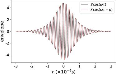
Figure 3. The effect of the variation of pulse phase φ(τ) over time is shown by the carrier wave under the typical hypersecant shape of a solitonic pulse. The blue curve for a pulse with finite φ(τ) is set against a yellow curve for a constant phase and shows that its oscillations are completed in advance to pulses free from environmental effects.
Download figure:
Standard image High-resolution imageSince the three factors in the integrands of equation (22) are either exponential or variants of exponential functions, the phase culminated on a pulse is a monotonically increasing function of time. This is evidenced by the plots of φ(τ) given as dashed curves in figure 4 for four different constant spectral densities γ. The rate of phase accumulation increases along with the increment of γ when Γ, regarded as a measure of rate of feedback from the environment is accordingly increased. The envelope area  computed from the integral of
  in equation (20) is plotted in the same figure, showing that the area variation accentuates on the range of time where the phase variation is minimal, thereby ratifying the assumptions we took above when arriving at the explicit solution of
  .
.

Figure 4. The pulse envelope area  (solid curves and scaled on the left axis) and the pulse carrier phase φ(τ) (dashed curves scaled on the right axis) are plotted as functions of local time τ over the same duration for the spectral densities γ = 4C0 = 5 MHz (blue curves), 50 MHz (yellow curves), 100 MHz (red curves), and 150 MHz (black curves).
Download figure:
Standard image High-resolution image
5. Conclusion
To conclude, we have taken an adiabatic master equation approach to analyze the propagation of a pulse through an environmentally coupled qubit. The qubit would be free from longitudinal relaxation when the pulse area is nπ. Further, when an orthogonal condition between the pulse phase and the bath spectral density is satisfied, the transverse relaxation also vanish during propagation. If the pulse area is 2nπ, the propagation becomes transparent. It is also proved that when relaxations are not vanishing, the thermal environment is responsible for inducing pulse ramifications which are frequently observed in SIT experiments. The approach has also enabled us for the first time to compute analytically the phase variation in the pulse during its propagation through a two-level system. Modeled on superconducting qubit circuits, the exact knowledge on pulse–qubit interactions would benefit the designs of more sophisticated microwave control pulses for quantum information processing.
Acknowledgments
Y-BG acknowledges the support of the National Natural Science Foundation of China under Grant No. 11674017. HI acknowledges the support by FDCT of Macau under Grants 065/2016/A2 and 0130/2019/A3, University of Macau under Grant MYRG2018-00088-IAPME, and National Natural Science Foundation of China under Grant No. 11404415.
Appendix A.: Adiabatic quantum master equation
To construct a master equation for the system when taking into account the geometric phases, we consider customarily a quantum heat bath consisting of a multimode resonator  having dipole-field interaction
  with the qubit.
Since the incident pulse with envelope  is a weak driving field to the qubit, the qubit evolution under the coupling strength
  could be regarded as an adiabatic process under Born–Oppenheimer approximation when compared to the thermal relaxing process under couplings
  . Under the total Hamiltonian

with HS'(τ) + HB regarded as the free energy, the adiabatic process is described by the master equation for the Universe  :
:

in interaction picture.  stands for the density matrix for the thermal bath. The system-bath interaction
  has been transformed to the adiabatic evolution frame with the double-time transformation
  being used for the historic Hamiltonian HI(τ − s) following the convention [41, 42].
As given in equation (5) in the main text, the unitary transformations involve the dressed basis defined at both the initial moment τ0 and the current moment τ or the historic moment τ − s. In practice, we unify the basis reference to time τ by inversing eigenstate definitions of equations (4) and (5), finding equation (7), i.e.

based on which we can also derive

During the adiabatic process, the bath variables aj and  stay relatively static while the operator σx relevant to the system is rotated. Therefore, the static σx in the dressed basis reads

Then following the qubit-field interaction using the unitary transformation equation (A.4), the operator during the interaction reads for any historic moment s:
where  , which includes the special case with s = 0.
The derivation of the microscopic master equations begins with tracing out the bath variables in the Liouville equation (A.2) of the Universe, giving

where the integration limit is modified following equation (9). We note that evoking the commutator generates the double-time operators  according to equation (6). Therefore, equipped with equation (A.6), we compute
and ![${\hat{\sigma }}_{x}\left(\tau -s\right){\hat{\sigma }}_{x}\left(\tau \right)={\left[{\hat{\sigma }}_{x}\left(\tau \right){\hat{\sigma }}_{x}\left(\tau -s\right)\right]}^{{\dagger}}$](https://content.cld.iop.org/journals/1367-2630/22/10/103041/revision2/njpabbca4ieqn69.gif) . At the long-term limit τ → ∞, equation (A.7) expands into four terms. In dealing with the first term, we consider
. At the long-term limit τ → ∞, equation (A.7) expands into four terms. In dealing with the first term, we consider
Note from the expression of equation (A.8) the double-time operator product would contribute multiple terms in the integral, but only those with the factor  would remain since the other terms containing the fast-oscillating exponential factors would vanish after the integration over long period. Consequently, since only this exponential factor involves in the integration over the variable s, all other factors about time τ do not participate in the integration and

where the last equation employs the definition of equation (12). The integral would become

When applying the same arguments to the other three terms in the expansion of the rhs of equation (A.7), we arrives at

Finally, seeing that  is given in the interaction picture of the adiabatic evolution, we note that for the conversion back to Schroedinger picture,
which is the Lindblad form of the master equation as in equation (11). Therefore, at resonance with zero detuning, θ = π/4 and the Lindbladian term assumes a minimal coefficient  , which can be further reduced depending on the historic values of φ(τ) as demonstrated in the main text. On the other hand, the absence of interference from the incident pulse corresponds to the limiting case of large detuning δ with
  , giving θ = 0 and thus a maximal Lindbladian coefficient γ(ω0). With this coefficient, the master equation resumes its standard form in the bare-state basis.
Appendix B.: Equations of envelope and phase
From the original Maxwell equation (16), the loss κ in the waveguide is assumed negligible. Then the so-called slowly-varying envelope approximation [36], that is  ,
,  , ∂φ/∂t ≪ ω, and ∂φ/∂x ≪ k for the electric field E(t);
  and
and  for the polarization P(t) can be taken. Thus when substituting the expressions of E(t) and P(t) (i.e. in the form of equation (1)), the second-order partial derivatives with respect to both time and space are regarded as negligible terms in comparison to the linear terms
  , etc. The Maxwell equation is essentially reduced to a first-order PDE.
When comparing the real and the imaginary parts of both sides of this PDE, one arrives at the coupled equations


for the envelope variable and the phase variable. For the local time τ = t − x/v, the two derivative operators on the left-hand side can be combined, i.e.

under which equations (B.1) and (B.2) become ODEs of one variable:


Rearranging the factors on two sides lead to equations (17) and (18). The equation of  still couples to that of φ(τ) through an implicit dependence in
  . To effectively decouple them, we consider the perturbative expansion of Γ(τ) of equation (15) in
  , i.e. letting φ assume the initial value φ(0) in the integral, which is valid under the adiabatic approximation. Consequently, the expression of equation (20) for the envelope can be regarded as its zeroth-order solution and its higher-order corrections can be obtained by substituting the solution of φ in equation (22) back into Γ(τ) in a consecutive manner.
Appendix C.: Solving for envelope and phase
Noticing that the sinusoidal factor in equation (14) is simply  , given the definition of the envelope area
  , we can write equation (19) as

Recognizing  and using the abbreviation
  , we arrive at the inverted pendulum equation

Since  , the equation can be rewritten as

Since two time variables  and Γ(τ) are on the rhs, we adopt the Born–Oppenheimer approximation to regard Γ(τ) as a slow-varying variable compared to
  such that formal integration can be carried out on both sides. We note that in current experiments the longitudinal relaxation time T1 have entered microsecond range [31–33] while the microwave pulse width in concern is in the range of tens of nanoseconds. The latter can be synthesized with modern waveform generators without difficulty. Hence, the validity of the assumption is experimentally guaranteed and carrying out the integration gives

Then taking the square root on both sides, one arrives at a first-order equation

whereby the  factor can be moved to lhs and we can formally solve for
  :
:

where τ0 is an arbitrary initial time of integration and C is the integration constant. Hence,

and letting  shows
shows  . Absorbing C into the exponential, we can simplify the above into

where  can be regarded as the delay time. Then, using the identity
 ![$\mathrm{sin}2\theta =2{\left[\mathrm{tan}\enspace \theta +1/\mathrm{tan}\enspace \theta \right]}^{-1}$](https://content.cld.iop.org/journals/1367-2630/22/10/103041/revision2/njpabbca4ieqn94.gif) , equation (C.5) can be written as
, equation (C.5) can be written as

which gives equation (20).
For the phase φ(τ), we substitute the decay factor equation (13) into equation (17) to get

which is an integro-differential equation, considering the expression of  in equation (20). Like described in the text, we simplify the consideration by reducing Γ(τ) to a linear dependence on time, writing Γ(τ) = 4C0(τ − τ0) and hence

Therefore, equation (C.10) reads
Then integrating both sides with respect to the local time τ yields equation (22).