From Probabilistic to Quantile-Oriented Sensitivity Analysis: New Indices of Design Quantiles


Department of Structural Mechanics, Faculty of Civil Engineering, Brno University of Technology, 602 00 Brno, Czech Republic
Symmetry 2020, 12(10), 1720; https://doi.org/10.3390/sym12101720
Submission received: 28 September 2020
/
Revised: 14 October 2020
/
Accepted: 15 October 2020
/
Published: 19 October 2020
(This article belongs to the Special Issue Symmetric and Asymmetric Data in Solution Models)
Abstract
:In structural reliability analysis, sensitivity analysis (SA) can be used to measure how an input variable influences the failure probability Pf of a structure. Although the reliability is usually expressed via Pf, Eurocode building design standards assess the reliability using design quantiles of resistance and load. The presented case study showed that quantile-oriented SA can provide the same sensitivity ranking as Pf-oriented SA or local SA based on Pf derivatives. The first two SAs are global, so the input variables are ranked based on total sensitivity indices subordinated to contrasts. The presented studies were performed for Pf ranging from 9.35 × 10⁻⁸ to 1–1.51 × 10⁻⁸. The use of quantile-oriented global SA can be significant in engineering tasks, especially for very small Pf. The proposed concept provided an opportunity to go much further. Left-right symmetry of contrast functions and sensitivity indices were observed. The article presents a new view of contrasts associated with quantiles as the distance between the average value of the population before and after the quantile. This distance has symmetric hyperbola asymptotes for small and large quantiles of any probability distribution. Following this idea, new quantile-oriented sensitivity indices based on measuring the distance between a quantile and the average value of the model output are formulated in this article.
1. Introduction
The reliability of building structures is influenced by inherent uncertainties associated with the material properties, geometry, and structural load variables to which the reliability measure is sensitive [1]. A common measure of reliability is the failure probability Pf, which is estimated using stochastic models [2]. Failure occurs when the load action is greater than the resistance. In this respect, the key issue is the identification of the significance of input random variables with regard to Pf.
Reliability-oriented sensitivity analysis (ROSA) consists of computing the sensitivity ranking of input variables ranked according to the amount of influence each has on Pf. It is argued that sensitivity analysis (SA) should be used “in tandem” with uncertainty analysis and the latter should precede the former in practical applications [3]. This can encumber the entire computational process, especially in cases of very small Pf.
Alternatively, the assessment of reliability can be performed by comparing the design quantiles of load and resistance [4,5]. A structure is reliable if the design resistance is greater than the design load action. One might ask, if the reliability assessment based on Pf can be replaced by a reliability assessment based on design quantiles, can the SA of Pf be replaced by the SA of design quantiles? For this purpose, new types of sensitivity indices oriented to both design quantiles and Pf can be investigated in engineering applications.
In civil engineering, classical Sobol SA (SSA) [6,7] is applied in the research of structural responses [8,9,10,11,12,13,14,15,16] or responses in geotechnical applications [17,18]. SSA is attractive for a number of reasons, e.g., it measures sensitivity across the whole input space (i.e., it is a global method), and it is capable of dealing with non-linear responses, as well as measuring the effect of interactions in non-additive models. However, SSA is based on the decomposition of variance of the model output, without a direct reference (only with partial empathy) to reliability [19].
Sobol indices in the context of ROSA can be derived as in [20], by introducing the binary random variable 1 (failure) or 0 (success) as the quantity of interest [21], where the basis of this transformation is the importance measure between Pf and conditional Pf defined in [22]. Indices can be derived in different variants, depending on whether the square of the importance measure [20] or the absolute value of the importance measure [23,24] is considered, but only the variant [20] after Sobol is based on decomposition, with the sum of all indices equal to one.
Both classical Sobol indices [6,7] and Sobol indices in the context of ROSA [20] are a subset of sensitivity indices subordinated to contrasts [25] (in short, Fort contrast indices). The general idea of Fort contrast indices [25] is that the importance of an input variable may vary, depending on what the quantity of interest is. Fort contrast indices define different types of indices based on a common platform, thus providing new perspectives on solving reliability tasks of different types.
It can be shown that Sobol indices in the context of ROSA [20] are Fort contrast indices [25] associated with Pf (referred to as contrast Pf indices in this article). Furthermore, it can be shown that the classical Sobol indices [6,7] are Fort contrast indices [25] associated with variance. In general, the type of Fort contrast index [25] varies, according to the type of contrast used. Contrast functions permit the estimation of various parameters associated with a probability distribution. By changing the contrast, SA can change its key quantity of interest. The contrast may or may not be reliability-oriented.
Fort contrast indices can be considered as global since they are based on changes of the key quantity of interest (Pf, α-quantile, variance, etc.) with regard to the variability of the inputs over their entire distribution ranges and they provide the interaction effect between different input variables. On the other hand, contrast functions account for the variability of the inputs regionally, according to the type of key quantity of interest, e.g., changes around the mean value are important for variance, changes around the quantile are important for the quantile, etc.
Standard [4] establishes the basis that sets out the way in which Eurocodes can be used for structural design. Although the concept of the probability-based assessment of structural reliability has been known about for a long time [5], new types of quantile-oriented SA have not yet been examined, in the context of structural reliability, at an appropriate depth. It can be expected that many of the reliability principles applied in [4] can be applied symmetrically in ROSA using new types of sensitivity indices to find new relationships. The introduced ROSA may be connected to decision-oriented methods [26] in areas of civil engineering, where decision-making under uncertainty is presently uncommon.
2. Probability-Based Assessment of Structural Reliability
Let the reliability of building structures be a one-dimensional random variable Z:
where X1, X2, …, XM are random variables employed for its computation. The classical theory of structural reliability [27] expresses Equation (1) as a limit state using two statistically independent random variables, the load effect (action F), and the load-carrying capacity of the structure (resistance R).
The variable that unambiguously quantifies reliability or unreliability is the probability that inequality (2) will not be satisfied. If Z is normally distributed, reliability index β is given as
where μZ is the mean value of Z and σZ is its standard deviation. By modifying Equation (3), we can express μZ −β·σZ = 0. The failure probability Pf can then be expressed as
where ΦU(·) is the cumulative distribution function of the normalized Gaussian probability density function (pdf). Reliability is defined as Ps = (1 − Pf). For other distributions of Z, β is merely a conventional measure of reliability. Equation (3) can be modified for normally distributed Z, F, and R as
where αF and αR are values of the first-order reliability method (FORM) sensitivity factors.
It can be noted that Sobol’s first-order indices are equal to the squares of αF and αR: SF = and SR = , respectively [19]. By applying αF and αR according to Equation (6), Equation (5) can be written with formally separated random variables as
Equation (7) is a function of the four statistical characteristics of μF, σF, μR, and σR, from which β, αF, and αR are computed. The left side in Equation (7) is the design load Fd (upper quantile) and the right side is the design resistance Rd (lower quantile).
3. Sensitivity Analysis
In structural reliability, the key quantities of interest are the failure probability Pf and the design quantiles Fd and Rd. In order to analyse the reliability, ROSA must be focused on the same key quantity of interest: Pf, Fd, and Rd. Local and global types of ROSA are applied in this article.
3.1. Local ROSA
The partial derivative δPf/δμxi with respect to the mean value μ of the input variable Xi presents a classical measure of change in Pf (see, e.g., [28,29,30,31,32]). The derivative-based approach has the advantage of being very efficient in terms of the computation time. There are two main disadvantages of using the derivative as an indicator of sensitivity.
The first disadvantage is that the derivative measures only change at the point (local SA) where it is numerically realized. If the algorithms on the computer are of the “black-box” type, then only a numerical evaluation of the derivative is possible. The second disadvantage is that a large absolute value of the derivative does not necessarily mean a large influence of the input on the output if the distribution range of the input variable is small compared to other variables.
A better proportional degree of sensitivity is obtained when the derivative is multiplied by the standard deviation σXi of the input variable.
The advantage of using Equation (9) is the inclusion of σXi and the possibility of introducing a correlation between the input random variables. A limitation of the derivative-based approach occurs when the analysed variable is of an unknown linearity.
Regarding quantiles, the use of partial derivatives as an indicator of sensitivity analogously to Equation (9) is not offered. For example, for the additive model X1 + X2, the derivative of the quantile with respect to the mean value is always equal to one. Conversely, in non-additive models, the derivative of the quantile with respect to the mean value may give very high or low values, and thus, the derivative of the quantile does not appear to be a useful measure of sensitivity.
3.2. Global ROSA
Global ROSA can be computed using Fort contrast indices [25], which implicitly depend on parameters associated with the probability distribution. In engineering applications, it is primarily the probability Pf [33,34], the design quantiles Fd and Rd [35], or the median [36].
Sensitivity indices subordinated to contrasts associated with probability (in short, contrast Pf indices) are based on quadratic-type contrast functions [25]. However, contrast Pf indices can be defined more easily based on the probability of failure and the conditional probabilities of failure [19]. A formula that does not require the evaluation of contrast functions can be used for practical computation. For practical use, the first-order probability contrast index Ci can be rewritten in the form of [19]
The sensitivity index Ci measures, on average, the effect of fixing Xi on Pf, where Pf = P(Z < 0) is the failure probability and Pf|Xi = P((Z|Xi) < 0) is the conditional failure probability. The mean value E[·] is taken over Xi. In Equation (10), the term Pf(1 − Pf) is derived for probability estimator θ* = Argmin ψ(θ) = Pf from the minimum of contrast :
where V (1Z<0) is the variance in the case where there are only two outcomes of 0 and 1, with one having a probability of Pf. The largest variance occurs if Pf = 0.5, with each outcome given an equal chance. The contrast function ψ(θ) = E(1Z<0 − θ)2 vs. θ is convex and symmetrical in the interval across the vertical axis θ*. The plot of Pf(1 − Pf) vs. Pf is a concave function with left-right symmetry. The contrast for conditional probability is expressed in a similar manner as (Pf|Xi)(1 − Pf|Xi).
The second-order sensitivity index Cij is computed similarly:
where Pf|Xi,Xj = P((Z|Xi,Xj) < 0) is the conditional failure probability for fixed Xi and Xj. E[·] is taken over Xi and Xj. The index Cij measures the joint effect of Xi and Xj on Pf minus the first-order effects of the same factors. The third-order sensitivity index Cijk is computed similarly:
where Pf|Xi,Xj,Xk = P((Z|Xi,Xj,Xk) < 0) is the conditional failure probability for fixed triples Xi, Xj, and Xk. The other indices are computed analogously. All input random variables are considered statistically independent. The sum of all indices must be equal to one:
Contrast Pf indices can also be derived by rewriting Sobol indices in the context of ROSA [21]. Estimating all sensitivity indices in Equation (14) can be highly computationally challenging and difficult to evaluate. For a large number of input variables, it may be better to analyse the effects of input variables using the total effect index (in short, the total index) CTi.
Pf|X~i = P((Z|X~i) < 0) is the conditional failure probability evaluated for a input random variable Xi and fixed variables (X1, X2,…, Xi–1, Xi+1,…, XM). The total index CTi measures the contribution of input variable Xi, including all of the effects caused by its interactions, of any order, with any other input variable. The total index CTi can also be computed if all sensitivity indices in Equation (14) are computed. For example, CT1 for M = 3 can be written as CT1 = C1 + C12 + C13 + C123.
The structural reliability can also be assessed using design quantiles (see, e.g., [37]). Sensitivity indices subordinated to contrasts associated with the α-quantile [25] (in short, contrast Q indices) are based on contrast functions of the linear type. The contrast function ψ associated with the α-quantile can be written with parameter θ as [25]
where Y is scalar (here, F or R). Equation (16) reaches the minimum if the argument θ is the α-quantile estimator θ* (here, Fd or Rd). The plot of contrast function ψ(θ) vs. θ is convex and, with some exceptions, asymmetric.
Equation (16) is not quadratic like the contrast associated with Pf, because the distance (Y − θ) is considered linear. The first-order contrast Q index is defined, on the basis of Equation (16), as
where the first term in the numerator (and denominator) is the contrast computed for the estimator of α-quantile θ* = Argmin ψ(θ). The second term in the numerator is computed analogously, but with the provision that Xi is fixed. E[·] is taken over Xi.
The second-order α-quantile contrast index Qij is computed analogously, but with the fixing of pairs Xi and Xj:
The third-order sensitivity index Qijk is computed similarly:
All input random variables are considered statistically independent. The sum of all indices must be equal to one:
The total index QTi can be written analogously to Equation (15) as:
where the second term in the numerator contains the conditional contrast evaluated for input random variable Xi and fixed variables (X1, X2, …, Xi–1, Xi+1, …, XM). Equation (21) is analogous to Equation (15), but for the quantile.
3.3. Specific Properties of Contrasts Associated with Quantiles
Can contrast indices Q be estimated more easily, without having to evaluate the contrast function from Equation (16)? Let us study Equation (16) using a simple case study, where Y has a Gaussian pdf:
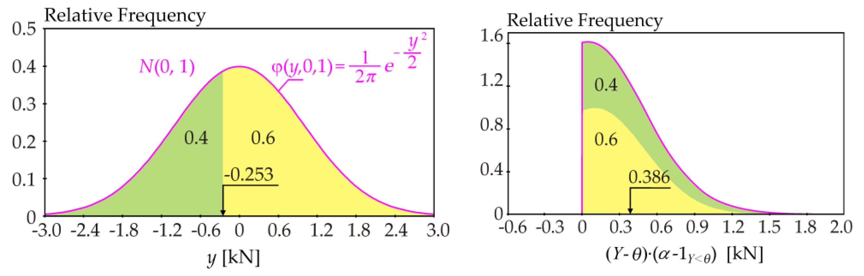
Figure 1 depicts an example of the evaluation of the contrast function for the 0.4-quantile of the normalized Gaussian pdf—Y ~ N(0, 1)—where the 0.4-quantile is θ* ≈ −0.253. The estimation of contrast function ψ(θ*) is based on the dichotomy of the pdf into two parts, separated by the α-quantile.
The value of the contrast function in Equation (16) is ψ(−0.253) = E((Y − (−0.253))(0.4−1Y<−0.253)) = 0.386, where the weight 0.6 favors the minority population over the 0.4-quantile and the weight 0.4 puts the majority population after the 0.4-quantile at a disadvantage. In this specific example, it can be observed that the function ψ(θ*) vs. θ* has an N(0, 1) course and therefore, ψ(−0.253) = ϕ(−0.253, 0, 1) = 0.386. In the case of the general Gaussian pdf Y ~ N(μ, σ2), function ψ(θ*) can be written in a specific form:
Equation (23) can only be used for estimates of contrast Q indices if Y has a Gaussian pdf; otherwise, Equation (23) has the form of an approximate relation. Another form of the sensitivity indices in Equation (20) derived from Equation (23) would be very practical; however, the conditional Gaussian pdf of Y, Gaussian pdf of Y|Xi, etc., makes the use of Equation (23) problematic in black box tasks, where skewness and kurtosis can have non-Gaussian values.
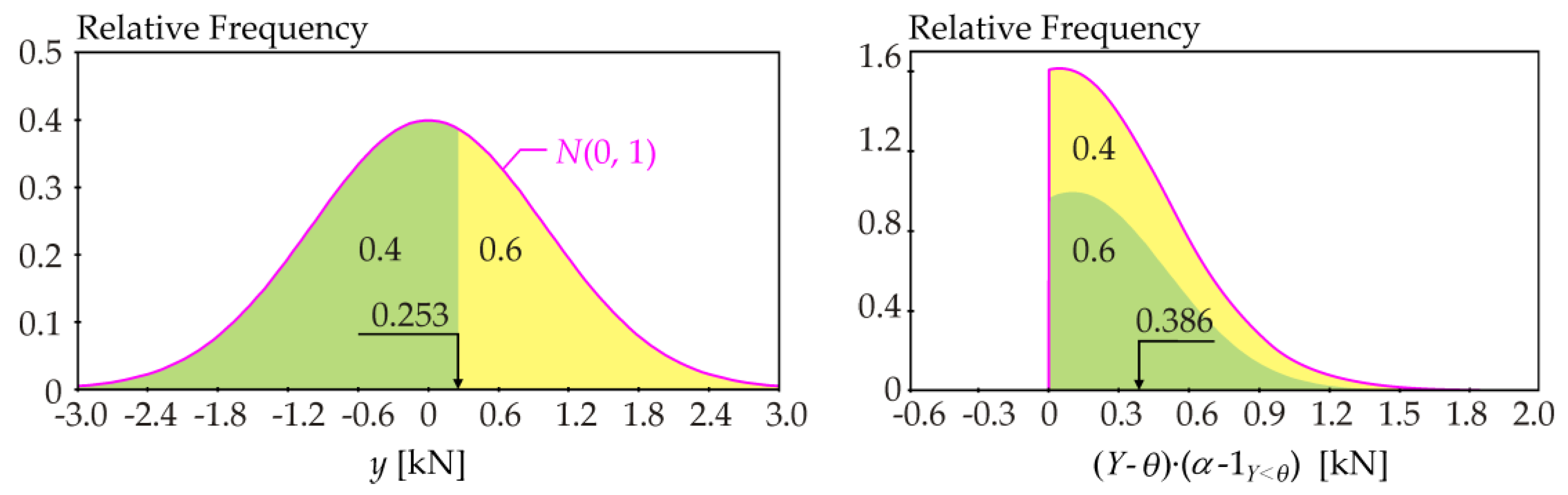
Due to the left-right symmetry of the Gaussian pdf in Figure 1, the same contrast function value can be obtained for the 0.6-quantile (see Figure 2).
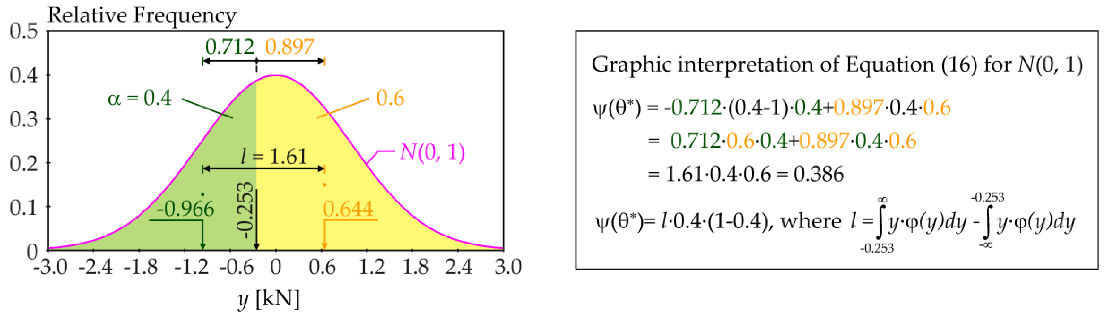
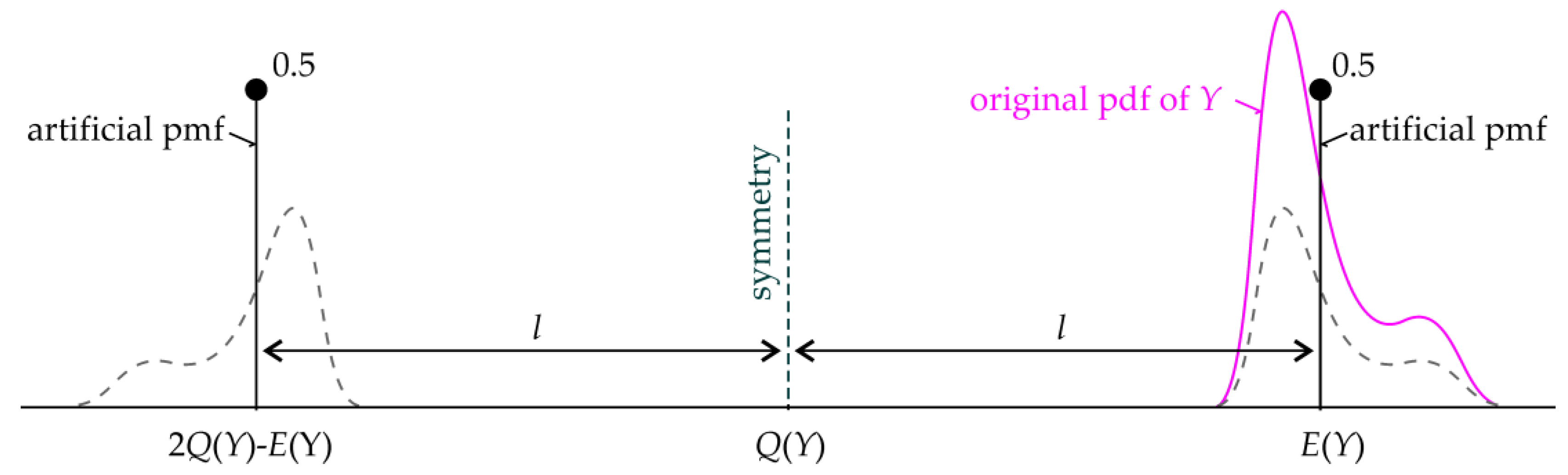
The following approach is more powerful. The value of contrast function ψ(θ*) can be expressed using the centers of gravity of the green and yellow areas (see Figure 3).
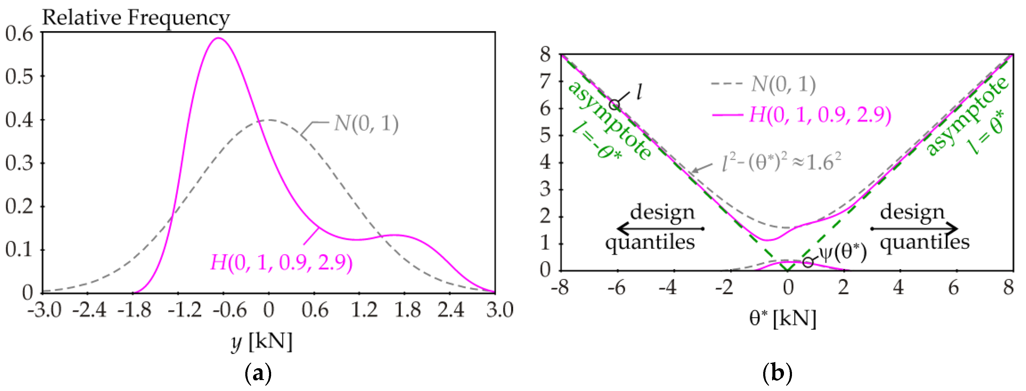
In the specific case of Y ~ N(0, 1), the dependence between l and θ* is a hyperbola l2 − (θ*)2 ≈ 1.62 with asymptotes l = ±θ* (see Figure 4). In a more general case of Y ~ N(μ, σ2), the dependence between l and θ* is a hyperbola l2 − (θ* − μ)2 ≈ σ2·1.62 with asymptotes l = ±(θ* − μ). The intersection of two asymptotes is at the center of symmetry of the hyperbola, which is the mean value μ = E(Y). The skewness and kurtosis (departure from the Gaussian pdf) lead to asymmetric and symmetric deviations from this hyperbola, but asymptotes of such a curve remain l = ±(θ* − μ). Figure 4 illustrates an example with the so-called Hermite pdf with a mean value of 0, standard deviation of 1, skewness of 0.9, and kurtosis of 2.9. Although deviations from the hyperbola are significant around the mean value, the dependence l vs. θ* approaches the asymptotes l = ±(θ* − μ) in the regions of design quantiles (see Figure 4b). The observation can be generalized to any pdf or histogram of Y.
For any pdf of f(y) of Y, an alternative form of the contrast function to Equation (16) can be derived in a new form:
where l is the distance of the centers of gravity of the two areas before and after the α-quantile (see the example in Figure 3). Sensitivity indices reflect change around the α-quantile estimator θ* using l while α is constant. Equation (24) is general for any pdf and offers new possibilities for evaluating contrast via l.
In general, SSA is relevant to the mean value of Y, while the SA of the quantile (QSA) is relevant to the α-quantile of Y. However, in many cases, there is a strong similarity between the conclusions of QSA and SSA if all or at least the total sensitivity indices are examined. It can be shown in a simple example of Y = X1 + X2 that corr(Q(Y|Xi), E(Y|Xi)) ≈ 1, where Q(Y|Xi) is the conditional α-quantile and E(Y|Xi) is the conditional mean value. Changing Xi causes synchronous changes in the α-quantile Q(Y|Xi) and mean value E(Y|Xi).
4. Case Study of the Ultimate Limit State
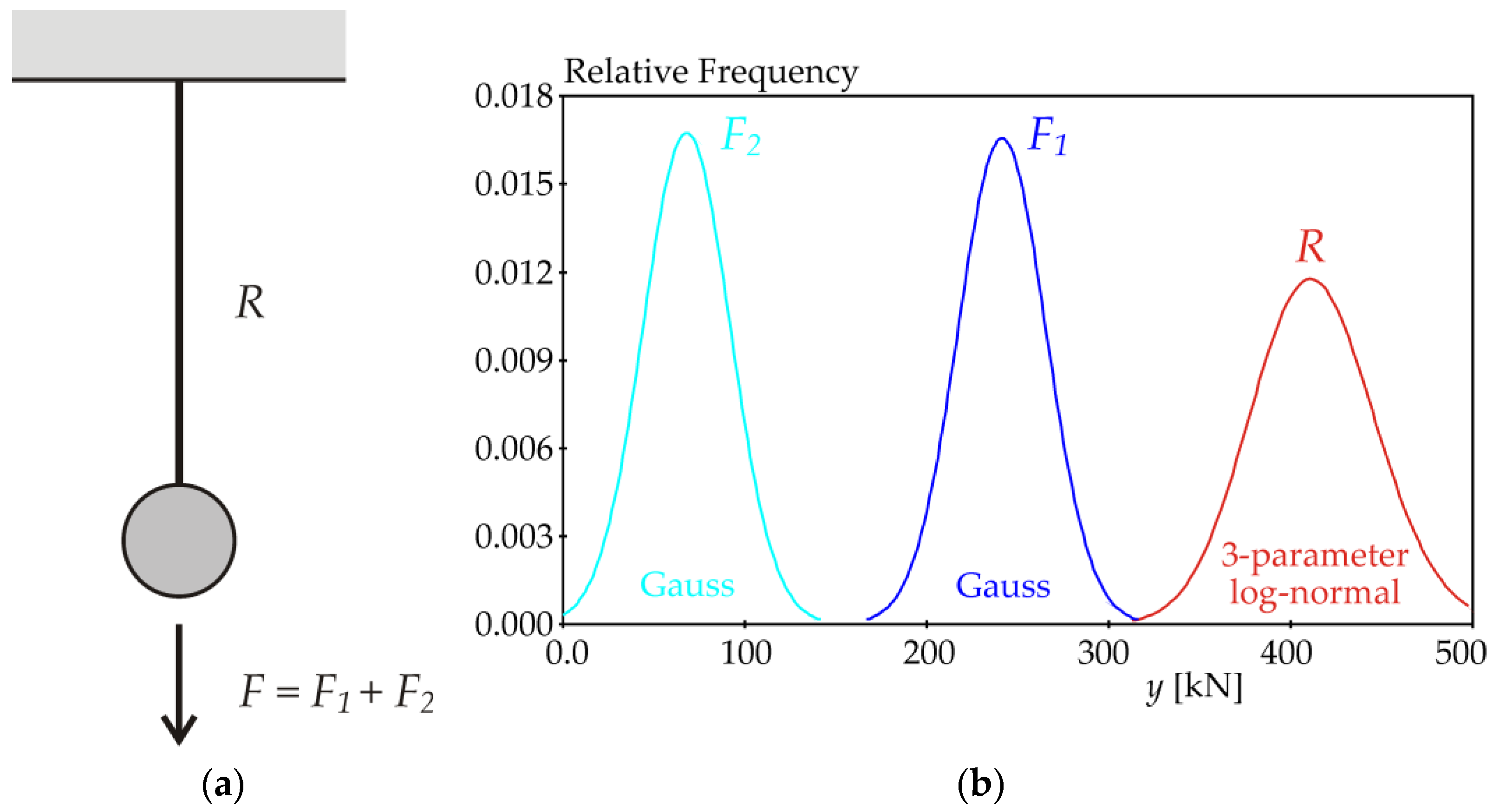
Probability-based reliability analysis considers a stochastic model of an ultimate limit state of a bar under tension (see Figure 5a). The structural member is safe when the sum of loads is less than the relevant resistance.
The bar is loaded by two statistically independent forces F1 and F2, both of which have a Gaussian pdf (see Figure 5b and Table 1). Parameter μP changes the mean value of the axial load of the bar, while the standard deviation of F is constant. The resulting force F = F1 + F2 has a Gaussian pdf with a mean value of = + = 309.56 kN + μP and standard deviation = ( + )0.5 = 33.94 kN.
The stochastic computational model for the evaluation of the static resistance R is a function of three statistically independent random variables: The yield strength fy; plate thickness t; and plate width b [40]:
where t·b is the cross-sectional area. The resistance R is a function of material and geometric characteristics fy, t, and b, whose random variabilities are considered according to the results of experimental research [41,42]. Random variables fy, t, and b are statistically independent and are introduced with Gaussian pdfs (see Table 2).
The arithmetic mean μR, standard deviation σR, and standard skewness aR of resistance R can be expressed using equations (see [40]), based on arithmetic means μfy, μt, and μb and standard deviations σfy, σt, and σb presented in Table 2.
The mean value of R can be written as
The standard deviation of R can be written as
The standard skewness of R can be written as
For example, for input random variables from Table 2, we can write μR = 412.68 kN, σR = 34.057 kN, and aR = 0.111.
Goodness-of-fit and comparison tests [40] have shown that probabilities down to 1 × 10⁻¹⁹ are estimated relatively accurately using the approximation of probability density R by a three-parameter lognormal pdf with parameters μR, σR, and aR. This approximation is also suitable when one variable in Equation (26) is fixed. Fixing two variables leads to R with a Gaussian pdf with parameters μR and σR.
In SA, the failure probability can be computed using distributions F (Gaussian) and R (three-parameter lognormal or Gaussian) as the integral:
where φF(y) is the pdf of load action, ΦR(y) is the distribution function of resistance, and y denotes a general point of the force (the observed variable) with the unit of Newton. The integration in Equation (30) is performed in the case study numerically using Simpson’s rule, with more than ten thousand integration steps over the interval [μZ − 10σZ, μZ + 10σZ].
5. Computation of Sensitivity Indices
The aim of SA in the presented case study is to assess the influence of input quantities F1, F2, fy, t, and b on the failure probability Pf or design quantiles Fd and Rd.
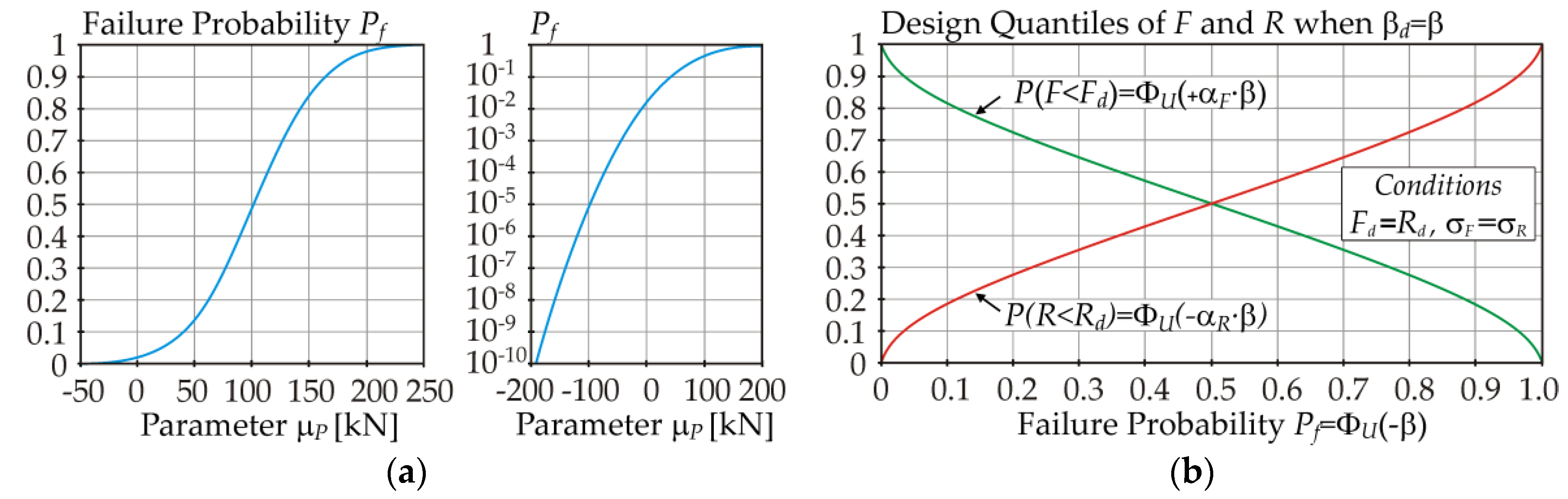
The numerical parameter of the case study is μP, which changes with the step ΔμP = 10 kN. Although μP is the computation parameter, sensitivity indices are preferably plotted, depending on Pf, because Pf has a clear relevance to reliability. The transformation of μP to Pf is expressed using Equation (30) (see Figure 6a).
In practice, the procedure is as follows: The value of μP is selected, the sensitivity indices and Pf are computed, and the indices vs. Pf are then plotted. If the design quantiles are the key quantities of interest, then the dependency between Pf and the probabilities of the design quantiles can be considered, according to Figure 6b.
In Figure 6b, the probability of design quantiles Fd and Rd is considered under the condition Fd = Rd in Equation (7) and σF = σR. Perfect biaxial symmetry of the curves in Figure 6b is only observed for perfect σF = σR; otherwise, the curve of the variable with the smaller standard deviation has a steeper slope. In the case study, for β = 3.8 (Pf = 7.2 × 10⁻⁵), P(F < Fd) = 0.9963, and P(R < Rd) = 0.0036, where Fd = Rd = 321.01 kN (μF = 229.97 kN, μR = 412.68 kN, and σF = 33.94 kN ≈ σR = 34.057 kN).
5.1. Local ROSA—Sensitivity Indices Based on Derivatives
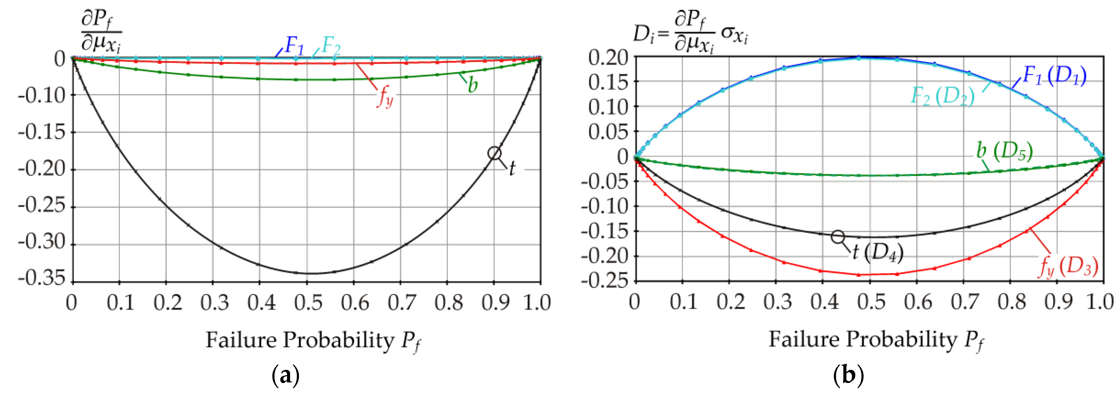
Figure 7a shows the partial derivatives of Pf with respect to the mean values μxi. Although the partial derivative of Pf with respect to μt has the greatest value, t is not the most influential input variable in terms of the absolute change of Pf due to the uncertainty (variance) of the input variable t. A better measure of sensitivity is obtained by multiplying the partial derivatives by the standard deviations of the respective input variables (see Figure 7b). Ranking according to Di gives the sensitivity ranking of input variables as fy, F1, F2, t, and b.
The plots in Figure 7 are approximately symmetrical about the vertical axis, but not perfectly symmetrical. The small amount of asymmetry is due to the small skewness of resistance R in Equation (1) (see Equation (29)). Perfect symmetry of the curves would occur if F and R had zero skewness (symmetric pdfs of both F and R).
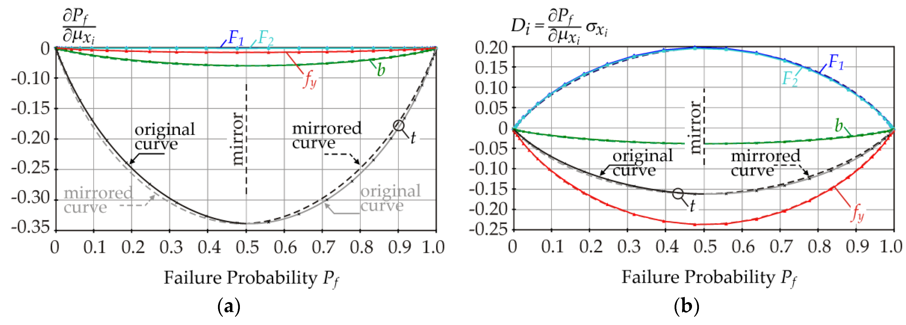
A small amount of asymmetry is graphically visible upon mirroring the solid curves to the dashed curves (see Figure 8). The dashed curves are artificial, showing the left-right asymmetry of the solid curves.
In Figure 8a, the dashed curves are lower than the solid curves on the left side of the graph. On the right side of the graph, the opposite is true. The same is observed in Figure 8b. A small amount of asymmetry occurs due to the small positive skewness of R. If R had a (theoretically) negative skewness, then the dashed curves would be higher than the solid curves on the left sides of each graph, and the opposite would be true on the right sides of the graphs.
5.2. Global ROSA—Contrast Pf Indices
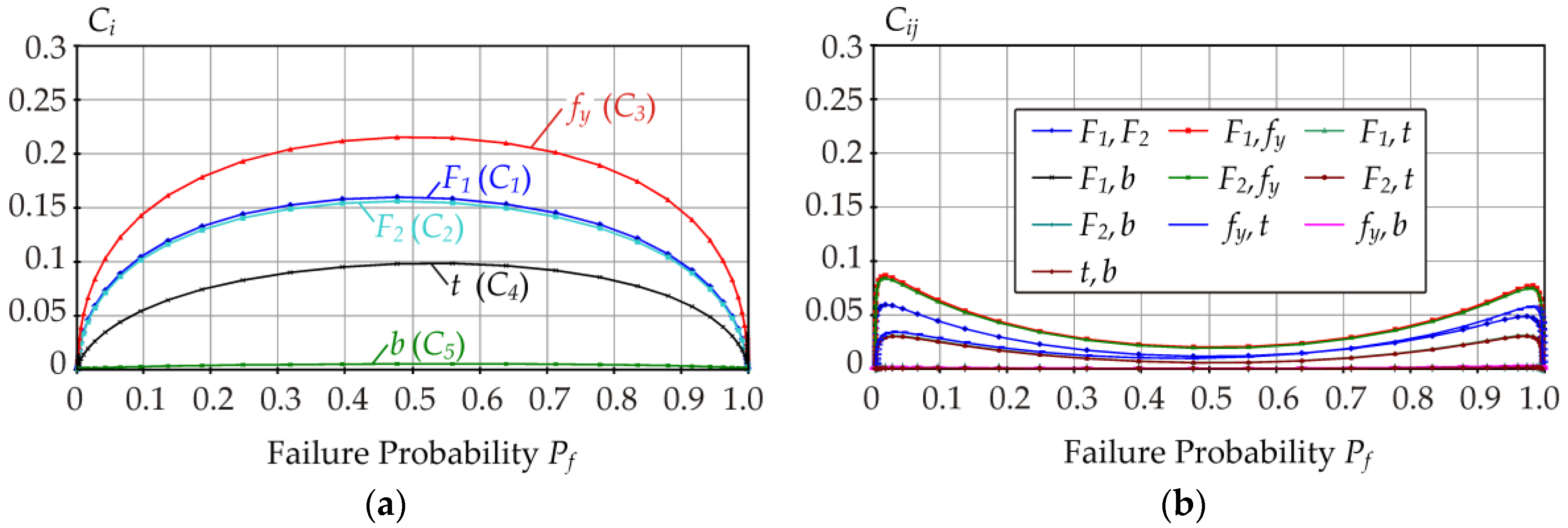
For the case study, contrast Pf indices are depicted in Figure 9, Figure 10, Figure 11, Figure 12 and Figure 13. All contrast Pf indices were computed numerically using Equation (30) for the interval Pf ∈ [9.35 × 10⁻⁸, 1–1.51 × 10⁻⁸].
In the interval Pf ∈[0.1, 0.9], the plot of Ci is a concave function with approximately left-right symmetry. The sum of indices C1 + C2 is the same as what would have been obtained had we introduced only one random variable for F with a Gaussian pdf with a mean value of μF = 309.56 kN +μP and standard deviation of σF = 33.94 kN: C2 + C1 = CF. The sum of indices C3 + C4 + C5 is the same as what would have been obtained had we introduced only one random variable for R with a three-parameter lognormal pdf with parameters μR = 412.68 kN, σR = 34.057 kN, and aR = 0.111: C3 + C4 + C5 = CR.
The slight asymmetry of the indices is of the same type as was described in the previous chapter for indices Di. For example, for Pf = 0.3, indices C1, C2, and C12 (load action) have slightly smaller values and indices C3, C4, C5, C34, C35, C45, and C345 (resistance) have slightly higher values, compared to the perfect symmetry. For the other indices, there is a mix of both influences.
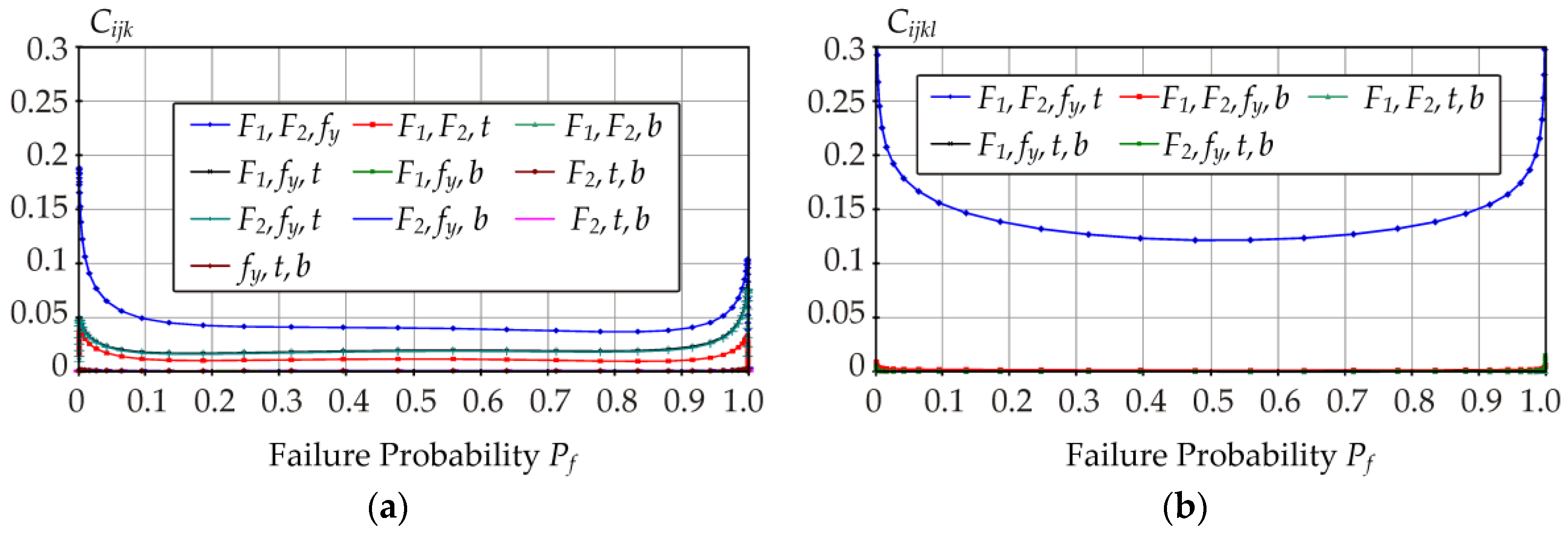
In the interval Pf ∈[0.1, 0.9], the first-, fourth-, and fifth-order indices generally have higher values than the second- and third-order indices.
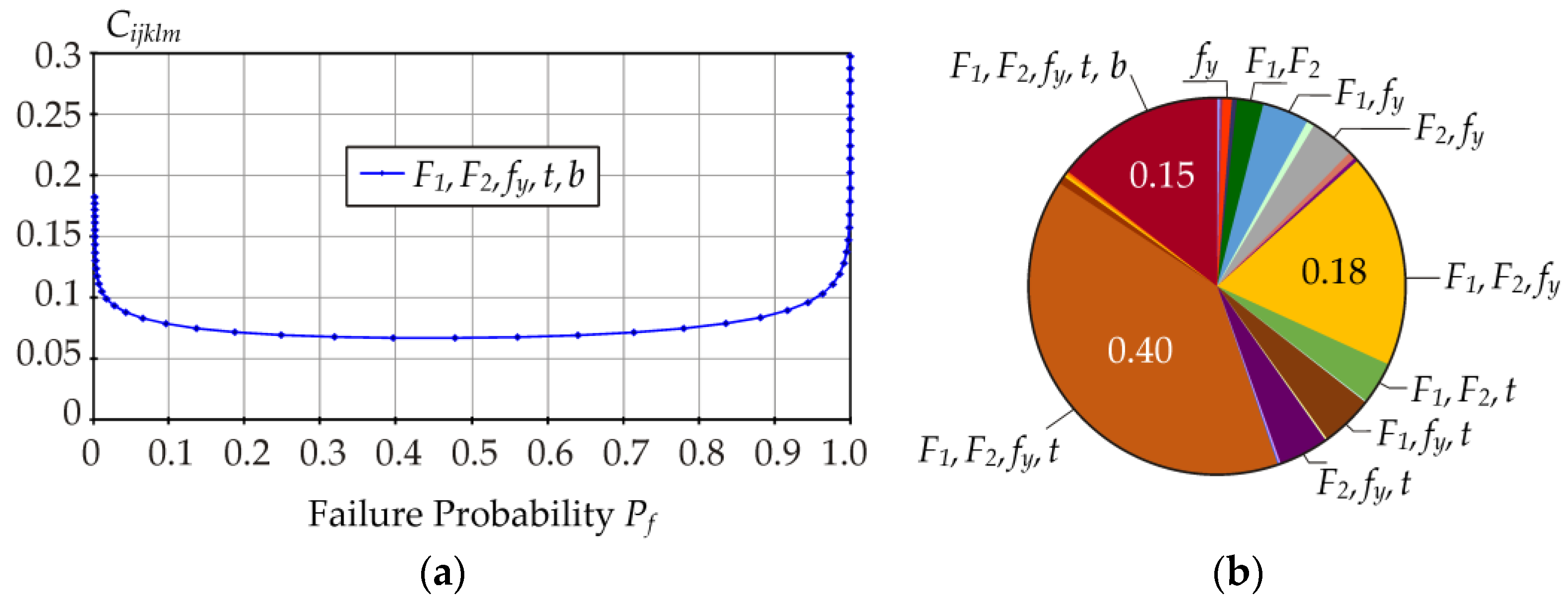
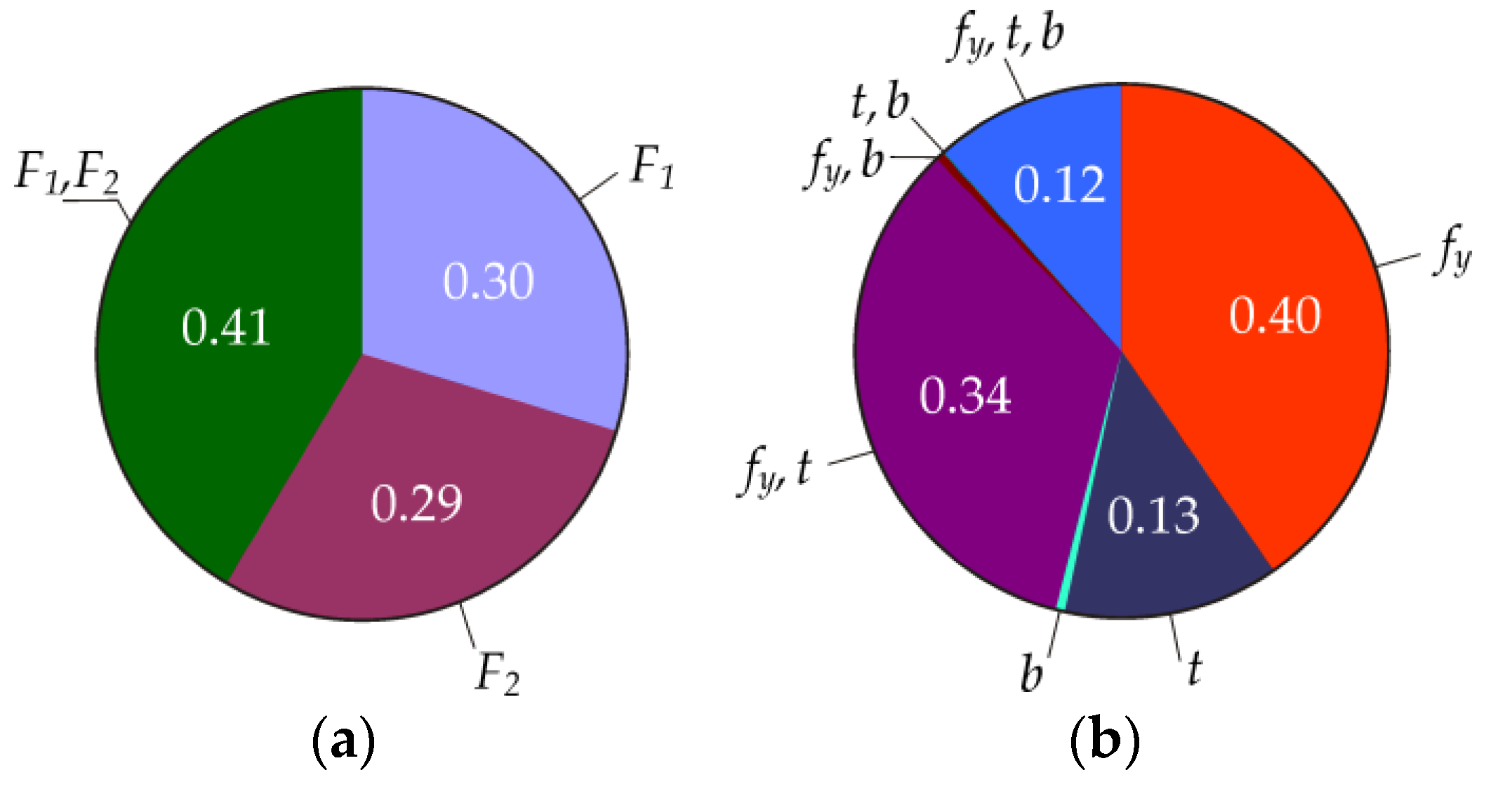
In civil engineering, the target values of Pf for reliability classes RC1, RC2, and RC3 taken from [4] are 8.5 × 10⁻⁶, 7.2 × 10⁻⁵, and 4.8 × 10⁻⁴ (also see [19]). Figure 11b shows the contribution of all 31 indices for target value Pf = 7.2 × 10⁻⁵. First-order indices are represented minimally, where ∑Si = 0.017. On the contrary, the representation of higher-order indices is significant, especially those related to fy, F1, and F2 (see Figure 11b).
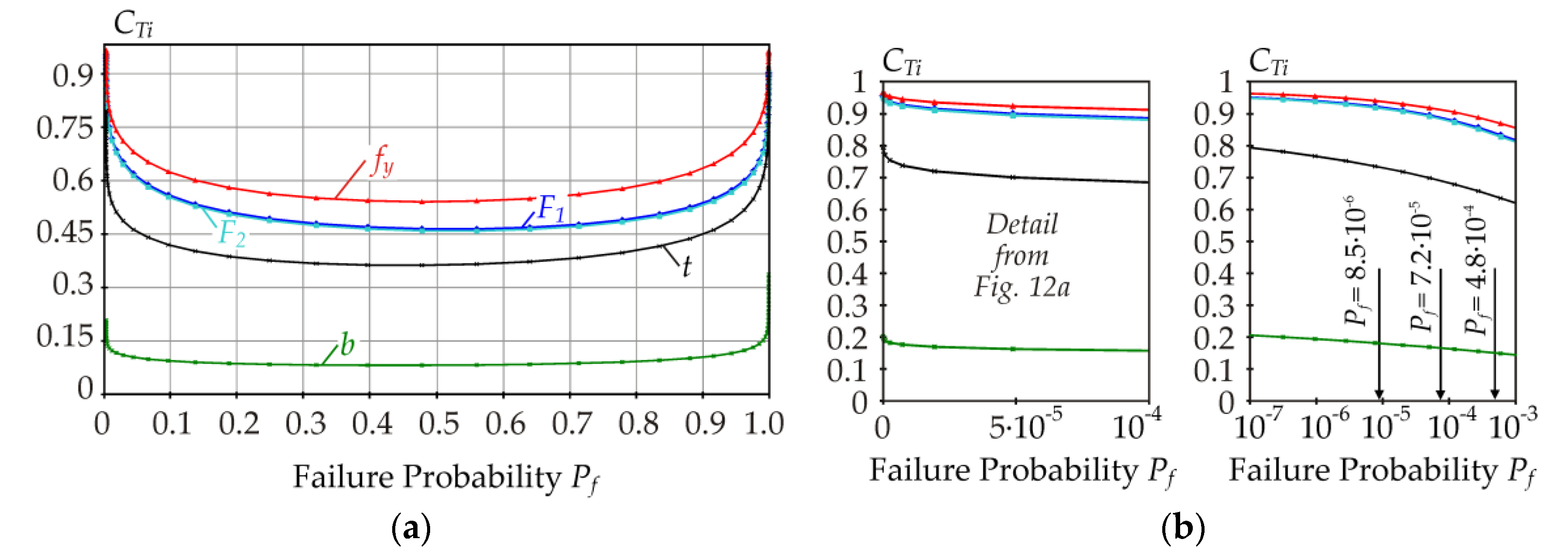
In Figure 11, fy occurs in all significant parts of the graph, but the same is true for F1 or F2. Determining the order of importance of input variables using 31 indices can be difficult. The use of total indices CTi is more practical. Input variables are ranked based on CTi as fy, F1, F2, t, and b (see Figure 12). This is the same ranking as was found using index Di (Figure 7b).
Figure 12b shows the total sensitivity indices for small Pf, which are relevant for the design of building structures. Figure 13 shows the local extremes of some sensitivity indices in the interval of small Pf. Interestingly, the sensitivity indices of small Pf have plots that are not obvious (cannot be extrapolated) from the plots in the interval Pf [0.1, 0.9]. Similar local extremes as in Figure 13 were not observed for Di in Figure 7.
5.3. Global ROSA—Contrast Q Indices
In the case study, contrast Q indices were estimated using the Latin Hypercube Sampling (LHS) method [43,44], according to the procedure in [35]. Indices Qi were estimated from Equation (17) using double-nested-loop computation. In the outer loop, E[·] was computed using one thousand runs of the LHS method. In the nested loop, conditional contrast values were computed using four million runs of the LHS method. The unconditional contrast value in the denominator was computed using four million runs of the LHS method. Higher-order indices were estimated similarly.
The target value Pf = 7.2 × 10⁻⁵ is considered according to [4]. In Equation (7), the design value of resistance Rd is considered as the 0.0036-quantile and the design load value Fd is considered as the 0.9963-quantile (see Figure 6). Sensitivity analysis is performed for R with a three-parameter lognormal pdf when no or one variable in Equation (26) is fixed; otherwise, a Gaussian pdf is used in the stochastic model.
It can be noted that standard design quantiles Fd = Rd = 321.01 kN computed using Equation (7) consider F and R with a Gaussian pdf. However, the design resistance value computed using a three-parameter lognormal pdf (stochastic model) is 325.00 kN. The small difference is because the skewness aR = 0.111 was neglected in Equation (7).
The SA results of the 0.9963-quantile of F are depicted in Figure 14a. Input random variables for F are considered according to Table 1, where the value of μP for Pf = 7.2 × 10⁻⁵ is μP = −79.592 kN. Input random variables for R are considered according to Table 2. The results of SA of the 0.0036-quantile of R are depicted in Figure 14b.
By computing total indices QT1 = 0.71, QT2 = 0.70 and QT3 = 0.86, QT4 = 0.59, and QT5 = 0.13, the order of importance of input variables can be determined as F1 and F2 and fy, t, and b. Variables F and R have the same weight in Equation (2) and therefore, the order of importance of all five input variables can be determined as fy, F1, F2, t, and b, based on the estimates of all QTi.
This is a typical example of how the ranking of input parameters based on total indices can give reliable results. The results are satisfactory, although ROSA is not evaluated directly using Pf; it is “only” based on the SA of design quantiles Rd and Fd.
In the presented study, the results for other values of the α-quantile are the same as in Figure 14. In practice, this means that the change in μP (generally a change in μF) is not reflected in the results of contrast Q indices.
6. New Sensitivity Indices of Small and Large Design Quantiles
6.1. The Asymptotic Form of Contrast Q Indices for Small and Large Quantiles
For small and large (design) quantiles, contrast Q indices can be rewritten using Equation (24) and the asymptotes of hyperbolic functions described in Chapter 3.3. The first-order contrast Q index can be rewritten as
By substituting the hyperbolic function l2 − (θ* − μ)2 = σ2· for l, we can obtain an approximate relation for Qi:
where Q(Y) = θ*, E(Y) = μ, and V(Y) = σ2. The non-dimensional parameter l0 can be calculated from Equation (25) as l0 = l2/σ2 at the point θ* = μ. However, the precise value of l0 is not important if |Q(Y)-E(Y)| is large and l0 does not affect the asymptotes. By substituting the hyperbolic functions with their asymptotes, Equation (31) can be simplified as
Using asymptotes, the index is independent of variance and l0. The second-order probability Q index can be rewritten analogously:
The third-order probability Q index can be rewritten analogously:
Equations (33)–(35) represent an asymptotic form of contrast Q indices that can be used for SAs of low and high quantiles. Higher-order contrast Q indices can be rewritten analogously. The sum of all indices thus estimated is equal to one.
In civil engineering, the design quantile of resistance tends to be less than the 0.01-quantile and the design quantile of load action tends to be greater than the 0.99-quantile [4]. The asymptotic form of contrast Q indices reveals the degree of sensitivity as the distance between the quantile and the average value.
In the case study presented here, the use of Equation (33)–(35) leads to practically the same results as shown in Figure 14b, but only when low and high quantiles are analysed; otherwise, the formulas cannot be used. The computation of indices eliminates the repeated evaluation of contrast functions in the second loop.
6.2. New Quantile-Oriented Sensitivity Indices for Small and Large Quantiles: QE Indices
In Equation (33) to (35), replacing the absolute values with squares (Q(Y) − E(Y))2, (Q(Y|Xi) − E(Y|Xi))2, etc., leads to new sensitivity indices, which we denote as QE indices. The new first-order quantile-oriented index is defined as
The new second-order QE index is defined as
The new third-order QE index is defined as
Sensitivity indices Ki, Kij, and Kijk were formulated via analogies to Equations (33)–(35) and were tested by numerical experiments using linear and non-linear Y functions and LHS simulations. Only low and high quantiles can be studied. The sum of the indices of all orders was equal to one in all cases. The total index KTi can be formulated analogously to Equation (21).
The new sensitivity indices can be explained using an analogy to Sobol sensitivity indices. The classical Sobol’s first-order sensitivity index has the form
Equation (36) can be interpreted using Equation (39). The key idea is to introduce l2 as a variance. Equation (36) can be rewritten analogously to Equation (39) in the form
where l is the standard deviation of the “artificial” two-point probability mass function (pmf) having left-right symmetry around quantile Q(Y) (see Figure 15). Half of the population is mirrored behind the quantile Q(Y) and replaced by a dot on each side of Q(Y). In SA, only low and high quantiles of Y can be analysed, indicating high l and low σY in unconditional and conditional pdfs.
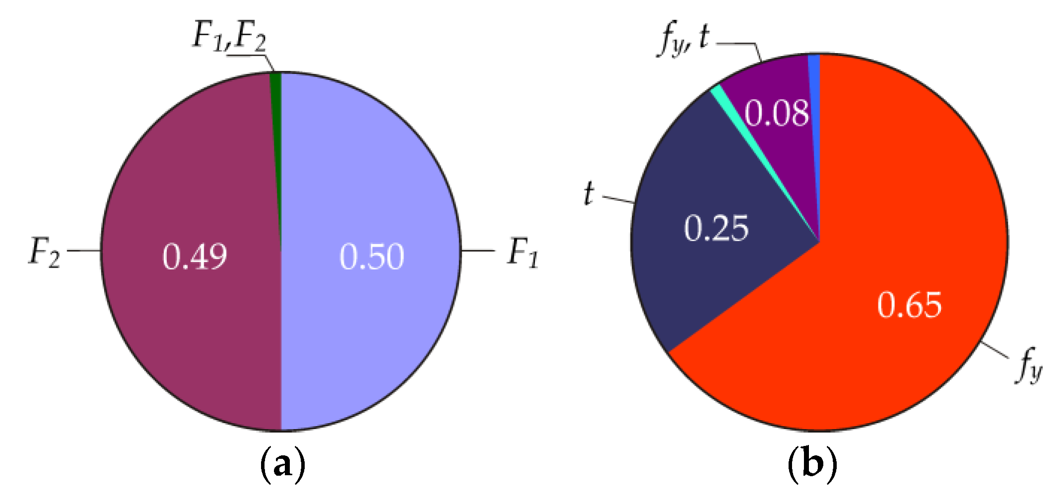
Let μP = −79.592 kN (Pf = 7.2 × 10⁻⁵). In the case study, QE indices were obtained on the load action side as K1 = 0.50, K2 = 0.49, and K12 = 0.01 and on the resistance side as K3 = 0.65, K4 = 0.25, K5 = 0.01, K34 = 0.08, K35 = 0.00, K35 = 0.00, and K345 = 0.01 (see Figure 16). By computing the total indices QT1 = 0.51, QT2 = 0.50 and QT3 = 0.74, QT4 = 0.34, and QT5 = 0.02, the order of importance of input variables can be determined as F1 and F2 and fy, t, and b. The sensitivity ranking based on all five QTi is fy, F1, F2, t, and b.
7. Discussion
In the case study, input variables were listed in decreasing order of sensitivity as fy, F1, F2, t, and b. Although the values of sensitivity indices of the different ROSA types vary, each ROSA gives the same sensitivity ranking:
- QT3 = 0.86 > QT1 = 0.71 > QT2 = 0.70 > QT4 = 0.59 > QT5 = 0.13;
- CT3 = 0.92 < CT1 = 0.892 < CT2 = 0.887 < CT4 = 0.69 < CT5 = 0.16;
- |D3| = 1.64 × 10⁻⁴ > |D1| = 1.52 × 10⁻⁴ > |D2| = 1.50 × 10⁻⁴ > |D4| = 1.02 × 10⁻⁴ > |D5| = 0.21 × 10⁻⁴;
- KT3 = 0.74 > KT1 = 0.51 > KT2 = 0.50 > KT4 = 0.34 > KT5 = 0.02.
These results were obtained for Pf = 7.2 × 10⁻⁵ and the corresponding design quantiles (see previous sections). Contrast Q and Pf indices of higher-orders have a significant share in both types of ROSA; therefore, key information is provided by total indices. Regarding the sensitivity ranking, the total indices of design quantiles are a good proxy of the total indices of Pf. However, the result cannot be generalized beyond the Gaussian (or approximately Gaussian) design reliability conditions.
The proposed SA concept is applicable in tasks where the reliability can be assessed by comparing two α-quantiles of two statistically independent variables analogous to R and F (see Equation (2)). The pdfs of R and F should be close to Gaussian (see Equation (8)), with condition σF ≈ σR. Then, ROSA can be effectively evaluated using the SA of design quantiles Rd and Fd, without having to analyse either Pf or the interactions between R and F. This is advantageous because estimates of contrast Q indices are usually numerically easier than estimates of contrast Pf indices, especially for small values of Pf.
For inequalities σF ≠ σR, the total indices of design quantiles should be corrected using weights based on the sensitivity factors αF and αR from Equation (6). For example, if σF → 0, then αF → 0 and αR → 1. When the influence of input variables on the load action side approaches zero, the reliability is only influenced by the variables on the resistance side. In the presented case study, the corrections of QTi indices are as follows: αF·QT1, αF·QT2, αR·QT3, αR·QT4, and αR·QT5. The correction of indices KTi can be performed similarly. If σF = σR, corrections are not necessary because αF = αF = 0.7071. Initial studies have shown the rationality of this approach; however, further analysis is necessary. Corrections of indices CTi are not performed. If σF → 0, then CTi of the variables on the load action side approaches zero naturally. If an extreme value distribution is used, such as a Gumbel or Weibull pdf [45,46], then the proposed concept cannot be used.
Contrast Q indices are based on measuring the fluctuations around the quantile, which is the distance l between the average value of the population before and after the quantile (see Figure 3). For low and high quantiles, contrast Q indices can be rewritten using asymptotes l = ±θ* of hyperbolic functions (see Figure 4). Although contrast Q indices do not have an analogy to the variance decomposition offered by Sobol’s indices through the Hoeffding theorem, studies of contrasts in applications [35,36] show some similarities between contrast Q indices and Sobol’s indices. The new QE indices and Sobol’s indices have formulas based on the squares of the distances from the average value and therefore, their comparison may be interesting in further work.
It can be noted that QE indices Ki, Kij, and Kijk give significant values of first-order indices Ki (compared to Qi) and relatively small values of higher-order indices, which is also a property observed in Sobol’s indices in the case study [35]. QE indices are based on quadratic measures of sensitivity like Sobol, but associated with quantiles. This domain deserves much more work in order to make QE indices a useful and practical tool.
All of the presented techniques are appropriate for SA of the stochastic model type considered in this article. For a general model, an important criterion is also the ease with which the SA can be performed. The most fundamental aspect of sensitivity techniques is local SA based on partial derivatives for computing the rate of change in Pf with respect to a given input parameter. Although the sensitivity ranking determined on the basis of Di is the same as from CTi, QTi, or KTi, this conclusion cannot be generalized, and Di is not suitable for application in every task. The one-at-a-time techniques are only valid for small variabilities in parameter values or linear computation models; otherwise, the partials must be recalculated for each change in the base-case scenario. In contrast, contrast-based SA does not have these limitations because computational models can generally be non-linear and sensitivity indices take into account the variability of inputs throughout their distribution range and provide interaction effects between different input variables.
The results of ROSA can be compared with traditional SA techniques, such as the correlation between input Xi and output Z. Spearman’s rank correlation coefficients are computed using one million LHS runs as corr(X1, Z) = −0.49, corr(X2, Z) = −0.48, corr(X3, Z) = 0.56, corr(X4, Z) = 0.38, and corr(X5, Z) = 0.08. The second traditional SA technique is SSA. Sobol’s first-order indices Si are computed according to Equation (39), using double-nested-loop computation [35], whereas the inner loop has four million runs and the outer loop ten thousand runs. The model output is Z. The values of Si are S1 = 0.25, S2 = 0.24, S3 = 0.34, S4 = 0.16, and S5 = 0.01. Sobol’s higher-order sensitivity indices are negligible. Both the correlation and SSA give the same sensitivity ranking as ROSA: fy, F1, F2, t, and b. The case study shows that the normalization of the newly proposed indices KTi leads to the classical Si, i.e., KTi/2.11 ≈ Si. Although correlations and Sobol’s indices are commonly used in SA of the limit states of structures, neither is directly reliability-oriented [19]. Further analysis of the relationship between the new QE indices and traditional Sobol indices is needed because it can provide new insights into the use of SSA in reliability tasks.
The dominance of the yield strength is an important finding for static tensile tests of steel specimens in the laboratory. In structural systems, the slender members under compression may be influenced by other initial imperfections, such as bow and out-of-plumb imperfections [9,10]. In a general steel structure, these imperfections can change the order of importance of the input random variables.
Symmetry is an important part of sensitivity indices and contrast functions (see, e.g., Equation (11) or Equation (24)). Reliability P~f = (1 − Pf) or unreliability Pf leads to the same contrast Pf indices, because Pf(1 − Pf) = P~f(1 − P~f). In the case study, the plots of the sensitivity indices were slightly asymmetric due to the small values of skewness of R. The plots of sensitivity indices vs. Pf would be perfectly symmetric in the case of a perfectly symmetric pdf of R and F, with zero skewness.
In the presented study, conclusions were made using SA subordinated to a contrast [25] and SA based on partial derivatives of Pf and new types of QE indices. Other types of SA of Pf like [47] or SA of the quantile [48] have not been studied. Numerous other types of sensitivity measures exist, such as [49,50,51,52,53,54,55,56,57,58,59], and it cannot be expected that the conclusions would be confirmed using any sensitivity index. The advantage of SA subordinated to a contrast is the use of a single platform (contrast) for the analysis of different parameters associated with a probability distribution.
8. Conclusions
This article has examined the relationships between the principles of semi-probabilistic reliability assessment of building structures according to the EN1990 standard and reliability-oriented sensitivity analysis (ROSA). The probability distributions of load and resistance close to Gaussian have been considered.
The article proposes new tools for performing ROSA. It has been shown that ROSA can be credibly evaluated using total indices of quantiles of resistance and load action, without the need to study the failure probability. ROSA of design quantiles gives the same sensitivity ranking as the two types of ROSA oriented to failure probability. Although this conclusion has been established based on one case study, the initial results suggest the possibility of using quantile-oriented ROSA in structural reliability studies. It should be interesting to develop a general approach for determining how to combine the various known indices, and in what order, in order to tackle a reliability task.
New quantile-oriented sensitivity indices denoted as QE indices have been formulated in the article. The first study showed that the distance between the quantile and the average value can be a very interesting measure of sensitivity, with the possibility of further development.
The apparent efforts to develop new types of sensitivity analyses show that the scientific community is still looking for the right combination of computational methods to solve specific problems. An important problem in structural reliability analysis is how to reduce the failure probability. Research focused on design quantities complements the development of failure probability estimation methods.
In engineering applications, the inclusion of quantile-oriented sensitivity analysis among the tools for assessing the effects of input variables on reliability makes it possible to effectively reduce the computational cost of sensitivity analysis of reliability with numerically demanding models. An example is the sensitivity analysis of design quantiles of numerous load cases, where the design quantile of the resistance of a structure only needs to be analysed once. It is worth noting that the specification of which parameters constantly appear close to the top of the list with the order of sensitivity is more important than the actual ranking. In practice, we can neglect the discrepancy between rankings for less important variables because these variables have a minimal or no effect on the reliability of structures.
Funding
The work has been supported and prepared within the project named “Influence of material properties of stainless steels on reliability of bridge structures” of The Czech Science Foundation (GACR, https://gacr.cz/), No. 20-00761S, Czechia.
Conflicts of Interest
The author declares no conflict of interest.
References
- Ditlevsen, O.; Madsen, H. Structural Reliability Methods; John Wiley & Sons Inc.: New York, NY, USA, 1996. [Google Scholar]
- Au, S.-K.; Wang, Y. Engineering Risk Assessment with Subset Simulation; Wiley: New York, NY, USA, 2014. [Google Scholar]
- Antucheviciene, J.; Kala, Z.; Marzouk, M.; Vaidogas, E.R. Solving civil engineering problems by means of fuzzy and stochastic MCDM methods: Current state and future research. Math. Probl. Eng. 2015, 2015, 362579. [Google Scholar] [CrossRef] [Green Version]
- European Committee for Standardization. EN 1990:2002: Eurocode—Basis of Structural Design; European Committee for Standardization: Brussels, Belgium, 2002. [Google Scholar]
- Joint Committee on Structural Safety (JCSS). Probabilistic Model Code. Available online: https://www.jcss-lc.org/ (accessed on 15 May 2020).
- Sobol, I.M. Sensitivity estimates for non-linear mathematical models. Math. Model. Comput. Exp. 1993, 1, 407–414. [Google Scholar]
- Sobol, I.M. Global sensitivity indices for nonlinear mathematical models and their Monte Carlo estimates. Math. Comput. Simul. 2001, 55, 271–280. [Google Scholar] [CrossRef]
- Kala, Z. Sensitivity assessment of steel members under compression. Eng. Struct. 2009, 31, 1344–1348. [Google Scholar] [CrossRef]
- Kala, Z. Sensitivity analysis of steel plane frames with initial imperfections. Eng. Struct. 2011, 33, 2342–2349. [Google Scholar] [CrossRef]
- Kala, Z. Global sensitivity analysis in stability problems of steel frame structures. J. Civ. Eng. Manag. 2016, 22, 417–424. [Google Scholar] [CrossRef]
- Kala, Z.; Valeš, J. Global sensitivity analysis of lateral-torsional buckling resistance based on finite element simulations. Eng. Struct. 2017, 134, 37–47. [Google Scholar] [CrossRef]
- Xiao, S.; Lu, Z.; Wang, P. Global sensitivity analysis based on distance correlation for structural systems with multivariate output. Eng. Struct. 2018, 167, 74–83. [Google Scholar] [CrossRef]
- Zamanian, S.; Hur, J.; Shafieezadeh, A. Significant variables for leakage and collapse of buried concrete sewer pipes: A global sensitivity analysis via Bayesian additive regression trees and Sobol’ indices. Struct. Infrastruct. Eng. 2020, 1–13. [Google Scholar] [CrossRef]
- Carneiro, G.D.; Antonio, C.C. Sobol’ indices as dimension reduction technique in evolutionary-based reliability assessment. Eng. Comput. Swans. 2020, 37, 368–398. [Google Scholar] [CrossRef]
- El Kahi, E.; Deck, O.; Khouri, M.; Mehdizadeh, R.; Rahme, P. Simplified probabilistic evaluation of the variability of soil-structure interaction parameters on the elastic transmission of ground movements. Eng. Struct. 2020, 213, 110554. [Google Scholar] [CrossRef]
- Jafari, M.; Akbari, K. Global sensitivity analysis approaches applied to parameter selection for numerical model-updating of structures. Eng. Comput. 2019, 36, 1282–1304. [Google Scholar] [CrossRef]
- Štefaňák, J.; Kala, Z.; Miča, L.; Norkus, A. Global sensitivity analysis for transformation of Hoek-Brown failure criterion for rock mass. J. Civ. Eng. Manag. 2018, 24, 390–398. [Google Scholar] [CrossRef]
- Xu, Z.X.; Zhou, X.P.; Qian, Q.H. The uncertainty importance measure of slope stability based on the moment-independent method. Stoch. Environ. Res. Risk Assess. 2020, 34, 51–65. [Google Scholar] [CrossRef]
- Kala, Z. Sensitivity Analysis in Probabilistic Structural Design: A Comparison of Selected Techniques. Sustainability 2020, 12, 4788. [Google Scholar] [CrossRef]
- Wei, P.; Lu, Z.; Hao, W.; Feng, J.; Wang, B. Efficient sampling methods for global reliability sensitivity analysis. Comput. Phys. Commun. 2012, 183, 1728–1743. [Google Scholar] [CrossRef]
- Li, L.; Lu, Z.; Feng, J.; Wang, B. Moment-independent importance measure of basic variable and its state dependent parameter solution. Struct. Saf. 2012, 38, 40–47. [Google Scholar] [CrossRef]
- Cui, L.; Lu, Z.; Fhao, X. Moment-independent importance measure of basic random variable and its probability density evolution solution. Sci. China Technol. Sci. 2010, 53, 1138–1145. [Google Scholar] [CrossRef]
- Xiao, S.; Lu, Z. Structural reliability sensitivity analysis based on classification of model output. Aerosp. Sci. Technol. 2017, 71, 52–61. [Google Scholar] [CrossRef]
- Ling, C.; Lu, Z.; Cheng, K.; Sun, B. An efficient method for estimating global reliability sensitivity indices. Probabilistic Eng. Mech. 2019, 56, 35–49. [Google Scholar] [CrossRef]
- Fort, J.C.; Klein, T.; Rachdi, N. New sensitivity analysis subordinated to a contrast. Commun. Stat. Theory Methods 2016, 45, 4349–4364. [Google Scholar] [CrossRef] [Green Version]
- Zavadskas, E.K.; Antucheviciene, J.; Vilutiene, T.; Adeli, H. Sustainable decision-making in civil engineering, construction and building technology. Sustainability 2018, 10, 14. [Google Scholar] [CrossRef] [Green Version]
- Freudenthal, A.M. Safety and the probability of structural failure. Trans. ASCE 1956, 121, 1337–1375. [Google Scholar]
- Melchers, R.E.; Ahammed, M. A fast-approximate method for parameter sensitivity estimation in Monte Carlo structural reliability. Comput. Struct. 2004, 82, 55–61. [Google Scholar] [CrossRef]
- Ahammed, M.; Melchers, R.E. Gradient and parameter sensitivity estimation for systems evaluated using Monte Carlo analysis. Reliab. Eng. Syst. Safe. 2006, 91, 594–601. [Google Scholar] [CrossRef]
- Millwater, H. Universal properties of kernel functions for probabilistic sensitivity analysis. Probabilistic Eng. Mech. 2009, 24, 89–99. [Google Scholar] [CrossRef]
- Wang, P.; Lu, Z.; Tang, Z. A derivative based sensitivity measure of failure probability in the presence of epistemic and aleatory uncertainties. Comput. Math. Appl. 2013, 65, 89–101. [Google Scholar] [CrossRef]
- Zhang, X.; Liu, J.; Yan, Y.; Pandey, M. An effective approach for reliability-based sensitivity analysis with the principle of Maximum entropy and fractional moments. Entropy 2019, 21, 649. [Google Scholar] [CrossRef] [Green Version]
- Kala, Z. Global sensitivity analysis of reliability of structural bridge system. Eng. Struct. 2019, 194, 36–45. [Google Scholar] [CrossRef]
- Kala, Z. Estimating probability of fatigue failure of steel structures. Acta Comment. Univ. Tartu. Math. 2019, 23, 245–254. [Google Scholar] [CrossRef]
- Kala, Z. Quantile-oriented global sensitivity analysis of design resistance. J. Civ. Eng. Manag. 2019, 25, 297–305. [Google Scholar] [CrossRef] [Green Version]
- Kala, Z. Benchmark of goal oriented sensitivity analysis methods using Ishigami function. Int. J. Math. Comput. Methods 2018, 3, 43–50. [Google Scholar]
- Jönsson, J.; Müller, M.S.; Gamst, C.; Valeš, J.; Kala, Z. Investigation of European flexural and lateral torsional buckling interaction. J. Constr. Steel Res. 2019, 156, 105–121. [Google Scholar] [CrossRef]
- Browne, T.; Fort, J.-C.; Iooss, B.; Le Gratiet, L. Estimate of quantile-oriented sensitivity indices. HAL 2017, hal-01450891. [Google Scholar]
- Maume-Deschamps, V.; Niang, I. Estimation of quantile oriented sensitivity indices. Stat. Probab. Lett. 2018, 134, 122–127. [Google Scholar] [CrossRef] [Green Version]
- Kala, Z. Limit states of structures and global sensitivity analysis based on Cramér-von Mises distance. Int. J. Mech. 2020, 14, 107–118. [Google Scholar] [CrossRef]
- Melcher, J.; Kala, Z.; Holický, M.; Fajkus, M.; Rozlívka, L. Design characteristics of structural steels based on statistical analysis of metallurgical products. J. Constr. Steel Res. 2004, 60, 795–808. [Google Scholar] [CrossRef]
- Kala, Z.; Melcher, J.; Puklický, L. Material and geometrical characteristics of structural steels based on statistical analysis of metallurgical products. J. Civ. Eng. Manag. 2009, 15, 299–307. [Google Scholar] [CrossRef]
- McKey, M.D.; Beckman, R.J.; Conover, W.J. Comparison of the three methods for selecting values of input variables in the analysis of output from a computer code. Technometrics 1979, 21, 239–245. [Google Scholar]
- Iman, R.C.; Conover, W.J. Small sample sensitivity analysis techniques for computer models with an application to risk assessment. Commun. Stat. Theory Methods 1980, 9, 1749–1842. [Google Scholar] [CrossRef]
- Nadarajah, S.; Pogány, T.K. On the characteristic functions for extreme value distributions. Extremes 2013, 16, 27–38. [Google Scholar] [CrossRef]
- Keshtegar, B.; Gholampour, A.; Ozbakkaloglu, T.; Zhu, S.-P.; Trung, N.-T. Reliability analysis of FRP-confined concrete at ultimate using conjugate search direction method. Polymers 2020, 12, 707. [Google Scholar] [CrossRef] [PubMed] [Green Version]
- Shi, Y.; Lu, Z.; Zhao, L. Global sensitivity analysis of the failure probability upper bound to random and fuzzy inputs. Int. J. Fuzzy Syst. 2019, 21, 454–467. [Google Scholar] [CrossRef]
- Kucherenko, S.; Song, S.; Wang, L. Quantile based global sensitivity measures. Reliab. Eng. Syst. Saf. 2019, 185, 35–48253. [Google Scholar] [CrossRef] [Green Version]
- Saltelli, A.; Ratto, M.; Andres, T.; Campolongo, F.; Cariboni, J.; Gatelli, D.; Saisana, M.; Tarantola, S. Global Sensitivity Analysis: The Primer; John Wiley & Sons: West Sussex, UK, 2008. [Google Scholar]
- Rykov, V.; Kozyrev, D. On the reliability function of a double redundant system with general repair time distribution. Appl. Stoch. Models Bus. Ind. 2019, 35, 191–197. [Google Scholar] [CrossRef]
- Shahnewaz, M.; Islam, M.S.; Tannert, T.; Alam, M.S. Flange-notched wood I-joists reinforced with OSB collars: Experimental investigation and sensitivity analysis. Structures 2019, 19, 490–498. [Google Scholar] [CrossRef]
- Douglas-Smith, D.; Iwanaga, T.; Croke, B.F.W.; Jakeman, A.J. Certain trends in uncertainty and sensitivity analysis: An overview of software tools and techniques. Environ. Model. Softw. 2020, 124, 104588. [Google Scholar] [CrossRef]
- Kaklauskas, A.; Zavadskas, E.K.; Radzeviciene, A.; Ubarte, I.; Podviezko, A.; Podvezko, V.; Kuzminske, A.; Banaitis, A.; Binkyte, A.; Bucinskas, V. Quality of city life multiple criteria analysis. Cities 2018, 72 Pt A, 82–93. [Google Scholar] [CrossRef]
- Lellep, J.; Puman, E. Plastic response of conical shells with stiffeners to blast loading. Acta Comment. Univ. Tartu. Math. 2020, 24, 5–18. [Google Scholar] [CrossRef]
- Medina, Y.; Muñoz, E. A Simple time-varying sensitivity analysis (TVSA) for assessment of temporal variability of hydrological processes. Water 2020, 12, 2463. [Google Scholar] [CrossRef]
- Mohebby, F. Function estimation in inverse heat transfer problems based on parameter estimation approach. Energies 2020, 13, 4410. [Google Scholar] [CrossRef]
- Strauss, A.; Moser, T.; Honeger, C.; Spyridis, P.; Frangopol, D.M. Likelihood of impact events in transport networks considering road conditions, traffic and routing elements properties. J. Civ. Eng. Manag. 2020, 26, 95–112. [Google Scholar] [CrossRef] [Green Version]
- Su, L.; Wang, T.; Li, H.; Cao, Y.; Wang, L. Multi-criteria decision making for identification of unbalanced bidding. J. Civ. Eng. Manag. 2020, 26, 43–52. [Google Scholar] [CrossRef]
- Szymczak, C.; Kujawa, M. Sensitivity analysis of free torsional vibration frequencies of thin-walled laminated beams under axial load. Contin. Mech. Thermodyn. 2020, 32, 1347–1356. [Google Scholar] [CrossRef] [Green Version]
Figure 1.
Example of the evaluation of Equation (16) for the 0.4-quantile of the Gaussian pdf.

Figure 2.
Example of the evaluation of Equation (16) for the 0.6-quantile of the Gaussian pdf.

Figure 3.
Graphical representation of the contrast in Equation (16) for the 0.4-quantile of N(0, 1).
Figure 3.
Graphical representation of the contrast in Equation (16) for the 0.4-quantile of N(0, 1).

Figure 4.
Plot of parameter l and function ψ(θ*) vs. the α-quantile θ*: (a) The Gaussian and non-Gaussian pdf; (b) The same asymptotes of hyperbolic and non-hyperbolic function.
Figure 4.
Plot of parameter l and function ψ(θ*) vs. the α-quantile θ*: (a) The Gaussian and non-Gaussian pdf; (b) The same asymptotes of hyperbolic and non-hyperbolic function.

Figure 5.
Static model: (a) Bar under tension and (b) probability density functions of R, F1, and F2 for μp = 0.
Figure 5.
Static model: (a) Bar under tension and (b) probability density functions of R, F1, and F2 for μp = 0.

Figure 6.
Probability of design α-quantiles vs. failure probability Pf: (a) μp vs. Pf; (b) Pf vs. α-quantiles.
Figure 6.
Probability of design α-quantiles vs. failure probability Pf: (a) μp vs. Pf; (b) Pf vs. α-quantiles.

Figure 7.
Derivative-based local SA of failure probability Pf: (a) Derivatives; (b) Sensitivity index Di.
Figure 7.
Derivative-based local SA of failure probability Pf: (a) Derivatives; (b) Sensitivity index Di.

Figure 8.
Derivative-based local SA of failure probability Pf: (a) Derivatives; (b) Sensitivity index Di.
Figure 8.
Derivative-based local SA of failure probability Pf: (a) Derivatives; (b) Sensitivity index Di.

Figure 9.
(a) First-order contrast Pf indices and (b) second-order contrast Pf indices.

Figure 10.
(a) Third-order contrast Pf indices and (b) fourth-order contrast Pf indices.

Figure 11.
(a) Fifth-order contrast Pf indices and (b) all-order contrast Pf indices for Pf = 7.2 × 10⁻⁵.
Figure 11.
(a) Fifth-order contrast Pf indices and (b) all-order contrast Pf indices for Pf = 7.2 × 10⁻⁵.

Figure 12.
Total contrast Pf indices: (a) All Pf and (b) low Pf.

Figure 13.
Details of contrast Pf indices for low Pf.

Figure 14.
Contrast Q indices: (a) 0.9963-quantile of F and (b) 0.0036-quantile of R.

Figure 15.
Introduction of l as the standard deviation of the two-point probability mass function.

Figure 16.
Contrast QE indices: (a) 0.9963-quantile of F ad (b) 0.0036-quantile of R.


Table 1.
The input random variables on the load action side.
| Characteristic | Index | Symbol | Mean Value μ (kN) | Standard Deviation σ |
|---|---|---|---|---|
| Load Action | 1 | F1 | 241.4 + 0.5·μP | 24.14 kN |
| Load Action | 2 | F2 | 68.16 + 0.5·μP | 23.86 kN |
Table 2.
The input random variables on the resistance side.
| Characteristic | Index | Symbol | Mean Value μ | Standard Deviation σ |
|---|---|---|---|---|
| Yield strength | 3 | fy | 412.68 MPa | 27.941 MPa |
| Thickness | 4 | t | 10 mm | 0.46 mm |
| Width | 5 | b | 100 mm | 1 mm |
Publisher’s Note: MDPI stays neutral with regard to jurisdictional claims in published maps and institutional affiliations. |
© 2020 by the author. Licensee MDPI, Basel, Switzerland. This article is an open access article distributed under the terms and conditions of the Creative Commons Attribution (CC BY) license (http://creativecommons.org/licenses/by/4.0/).
Share and Cite
MDPI and ACS Style
Kala, Z. From Probabilistic to Quantile-Oriented Sensitivity Analysis: New Indices of Design Quantiles. Symmetry 2020, 12, 1720. https://doi.org/10.3390/sym12101720
AMA Style
Kala Z. From Probabilistic to Quantile-Oriented Sensitivity Analysis: New Indices of Design Quantiles. Symmetry. 2020; 12(10):1720. https://doi.org/10.3390/sym12101720
Chicago/Turabian StyleKala, Zdeněk. 2020. "From Probabilistic to Quantile-Oriented Sensitivity Analysis: New Indices of Design Quantiles" Symmetry 12, no. 10: 1720. https://doi.org/10.3390/sym12101720
Note that from the first issue of 2016, this journal uses article numbers instead of page numbers. See further details here.