Nonlinear System Stability and Behavioral Analysis for Effective Implementation of Artificial Lower Limb


1
Narula Institute of Technology, Kolkata 700109, India
2
Indian Institute of Information Technology Kalyani, Kalyani 741235, India
3
JIS College of Engineering., Kalyani 741235, India
4
Department of Industrial Engineering, Yonsei University, Seoul 03722, Korea
*
Author to whom correspondence should be addressed.
Symmetry 2020, 12(10), 1727; https://doi.org/10.3390/sym12101727
Submission received: 8 September 2020
/
Revised: 6 October 2020
/
Accepted: 14 October 2020
/
Published: 19 October 2020
Abstract
:System performance and efficiency depends on the stability criteria. The lower limb prosthetic model design requires some prerequisites such as hardware design functionality and compatibility of the building block materials. Effective implementation of mathematical model simulation symmetry towards the achievement of hardware design is the focus of the present work. Different postures of lower limb have been considered in this paper to be analyzed for artificial system design of lower limb movement. The generated polynomial equations of the sitting and standing positions of the normal limb are represented with overall system transfer function. The behavioral analysis of the lower limb model shows the nonlinear nature. The Euler-Lagrange method is utilized to describe the nonlinearity in the field of forward dynamics of the artificial system. The stability factor through phase portrait analysis is checked with respect to nonlinear system characteristics of the lower limb. The asymptotic stability has been achieved utilizing the most applicable Lyapunov method for nonlinear systems. The stability checking of the proposed artificial lower extremity is the newer approach needed to take decisions on output implementation in the system design.
1. Introduction
Generally, nature is nonlinear as the responses of the physical systems in the applied fields also show nonlinear behavior. Some electromechanical processes show nonlinear behavior. Nonlinear controller can compensate the unwanted effects on the system. An important research field for nonlinear control systems is to design controllers to deal with uncertainty, mainly due to the unavailability of parametric information of the models and external disturbances. Hard nonlinearities such as dead-zones, hysteresis and saturation do not permit linear approximation of real-world systems. The method of approximation deals with the effects of nonlinearity. This can cause inaccuracy in the system. The effects of unwanted nonlinearities in the system should be analyzed to improve the dynamic performance of any real-time system development.
The applicability of forward dynamics [1] in the nonlinear systems such as lower limb models has a great impact on motion analysis. The application of Euler-Lagrange [2,3] method has been presented in the field of robotics for the movement analysis. The mathematical explanation of the systems is the newer approach using the Euler-Lagrange method to show the artificial motion [4]. There are many interesting applications of system performance analysis through mathematical model simulation in nonlinear domains, such as walking robots, Degree of Freedom (DoF) manipulator [5] working as an artificial limb, etc. The analysis and design of nonlinear control system stability has been discussed to give an overall idea to implement on different types of applications. This idea [6] has been implemented in the lower limb system performance analysis in the present work of the paper. The improvement of system stability [7] regarding robustness and control parameters should be taken into consideration to meet the need of the system design, which is incorporated in the biomedical field for human limb performance analysis. Asymptotic stability analysis from polynomials of the system to the Lyapunov method is investigated through a computational technique. The novel approach has been utilized for the system stability analysis [8] of the lower extremity design. Basic theoretical knowledge and stability-related methodology is discussed for the nonlinear systems [9]. Linearization of differential equations and phase portrait analysis of nonlinear systems has been shown in the nonlinear domain [10]. Exponential stability analysis and design of sampled-data nonlinear systems has been shown here [11]. The nonlinear system stability has been covered using the Lyapunov stability system. The most suitable stability checking method for nonlinear systems [12,13] is involved in the lower limb stability checking purpose in this present work. Stability criteria of nonlinear systems with associated features are discussed by Z. Roberto [14]. Information about Lyapunov stability analysis of nonlinear systems has been illustrated in the paper [15]. Overview of recent research works related to nonlinear system stability in different fields have been given [16]. Jacobian matrix formation for linearization of nonlinear systems with equilibrium point [17] detection has been discussed, which is implemented in the lower limb system stability analysis. The method of linearization, Lyapunov stability and Popov criteria for stability analysis of nonlinear systems have been mentioned [18]. Information on the describing function [19] related to nonlinear system behavioral analysis using a simulation approach has been discussed as the most interesting field to involve in the lower limb system behavioral analysis in the research work of this paper. Formalization of the limit cycle prediction depending on the nonlinear element by describing function is presented with great importance in the field of the system’s nature prediction [20]. The basics of describing function is discussed to predict the limit cycle [21]. The analysis of nonlinear systems based on the describing function, which is dependent on the different types of controllers such as proportional-Integral etc., are the base of the system characteristics determination as mentioned in the current work of research [22].
This approach to nonlinear control system stability determination has been chosen to incorporate the idea of the behavioral analysis of the system. The model of the lower limb of human beings is the main concern to be built representing the nonlinear system. Through some specific features, the implementation of system identification regarding forward dynamics and model generation is possible. The determination of stability in the nonlinear domain [23,24] preferably nourishes the idea of the planning of artificial limb [25,26] design. Until now, it has not been reported in any open journal that lower limb system stability can be analyzed using a nonlinear stability analysis method [27,28] in the field of bio robotics.
2. Forward Dynamics of the Artificial Lower Limb Movement
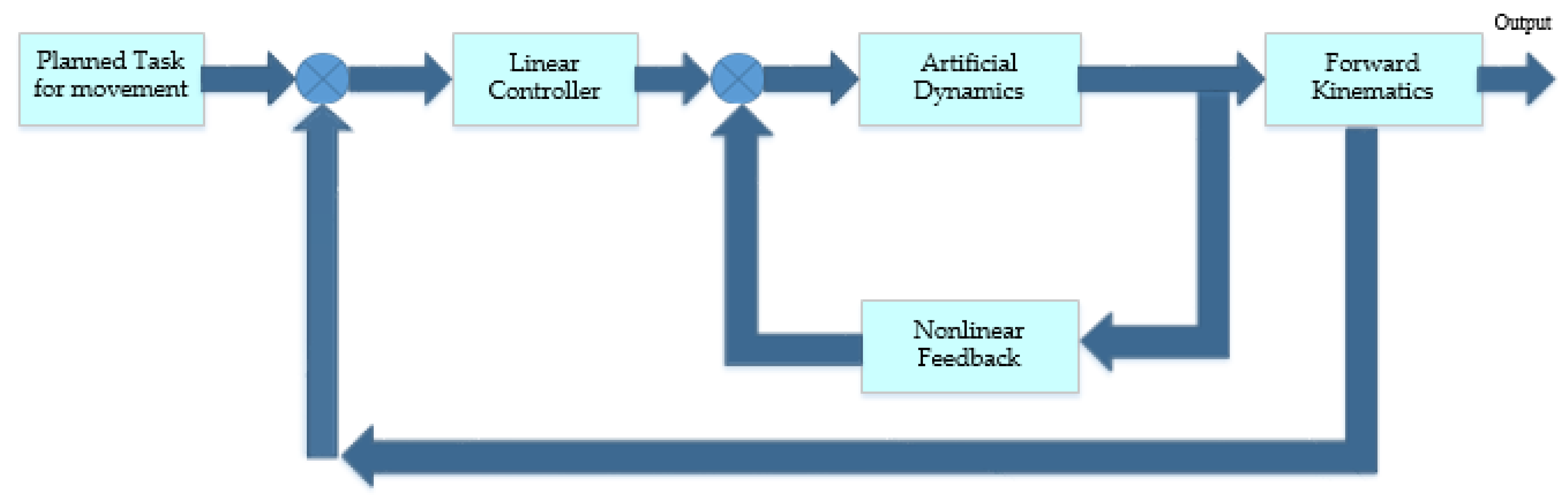
Forward dynamics [29] is the connection between the forces applied on a robotic mechanism and the produced accelerations, which is presented in Figure 1. Robot dynamics [30] is the application of rigid-body dynamics to robots. Forward dynamics [2] gives the forces and work out of the accelerations.
- Suppose, Joint position (Knee or ankle) of the artificial lower limb =
- Joint force of the lower limb =
- Joint velocity of the lower limb =
- Joint acceleration of the lower limb =
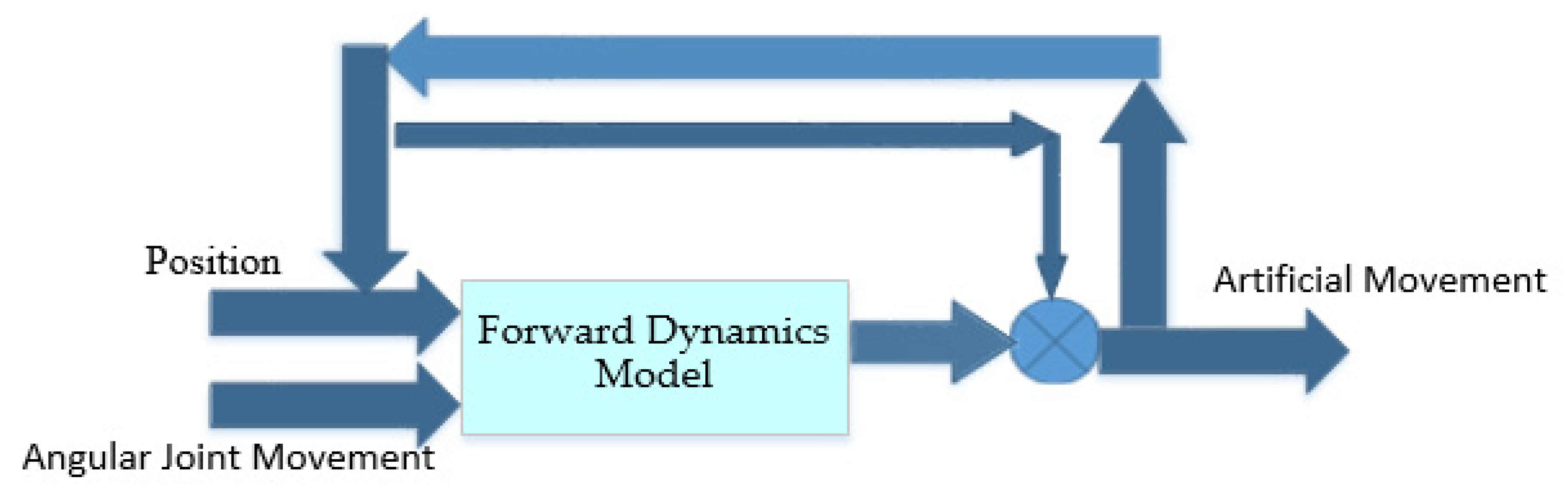
The Lagrangian approach delivers the immediate reduction in the characteristic size to solve many equations. This describes the equation of motion. The Lagrange formulation is used to avoid the acceleration finding as shown in Figure 2. The Lagrangian equation can be expressed as the difference between the kinetic energy and the potential energy as shown in the Equation (1).
where, Kinetic energy = and Potential energy = .
Euler-Lagrange equations are suitably obtained for the nonlinear behavioral analysis of the artificial movement of the lower limbs.
The Euler—Lagrange equation [3] is given below in Equation (2).
where,
- time derivative of partial derivative of L with respect to
- partial derivative of L with respect to
- power produced by the joints related to .
In the form of vector components, it can be written as shown in Equation (3).
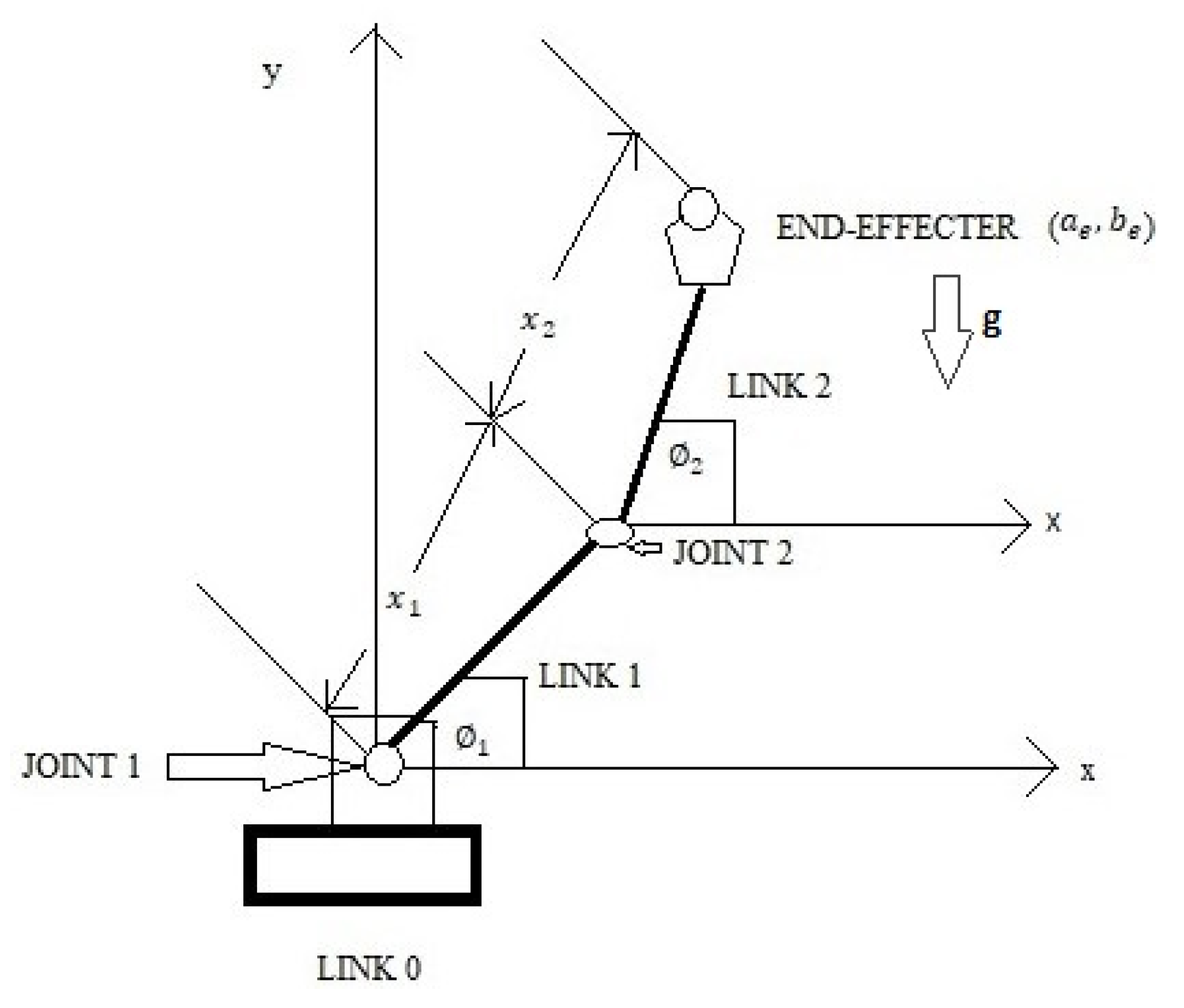
The joint1 refers to the ankle joint and the joint2 refers to the knee joint in Figure 3. From the above diagram, as shown in the Figure 3, Equation (4) can be written for the position of joint2 ().
where, = length of the limb from joint1 () to joint2.
The derivative of is expressed in Equation (5).
Similarly, it can be written for the position of end-effector () as shown in the Equation (6)
This equation is for the position and velocity of the model as shown in Equation (7).
where, = length of the limb from joint2 to end-effector.
Now, the Kinetic Energy for link1 and link2 are shown in the Equations (8) and (9) respectively.
where,
- = mass of the joint2,
- velocity of the joint2.
Now, the potential energy for link1 and link2 are as given in Equations (10) and (11),
Now,
where, .
One component of Lagrangian is as shown in the Equation (14).
Therefore,
The effect of on the 2nd joint torque is as given below in Equation (15).
Now torque for first joint is
Now torque for second joint is
Some terms are not dependent on the joint acceleration and velocity. So, the torque can be expressed as shown in Equation (19).
where,
- mass matrix shown in Equation (20)
- = velocity product term shown in Equation (21)
- gravity term, i.e., gravity due to springs in the mechanical model for potential energy is shown in Equation (22).
The overall acceleration depends not only on the joint accelerations but also on the products of the joint velocities. Joint coordinates are non-inertial. These velocity product terms appear because joint coordinates are non-inertial.
3. Experimental Methods
3.1. Stability Analysis of the Non-Linear System
The dynamic behavior of the artificial lower extremity model shows nonlinearity. The postures such as sitting and standing conditions of the lower part of human body exhibits the nonlinear characteristics. The control system [31,32,33] involves the mathematical relationship related to the nonlinear properties such as equilibrium point, saturation, dead zone, hysteresis, describing function, etc. Nonlinear systems may not produce a specific solution for all times but gives a decision maker feature [34,35] of the analyzed system. Through phase portrait analysis and the Lyapunov method, the system stability [36,37] of the designed system definition is feasible. Thus, system design method for nonlinear control systems are application-specific [38]. The describing function is the well-established process to analyze the nonlinear function [39] with an approximation, and to determine the stability of a nonlinear system. It is basically the approximated extended version of frequency domain analysis. For a higher degree of nonlinearity, the describing function is used but no information about time domain such as steady state error is given by this. Phase plane analysis can be used, but the order of the system should be less than second order as it is a graphical system. Sometimes it is called a sinusoidal describing function.
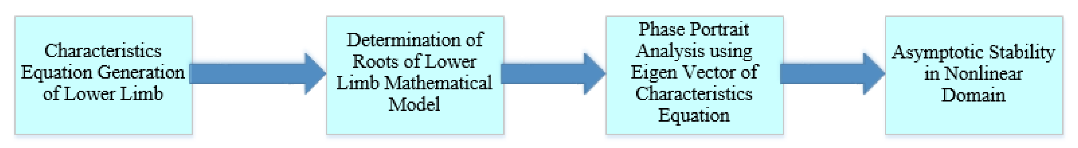
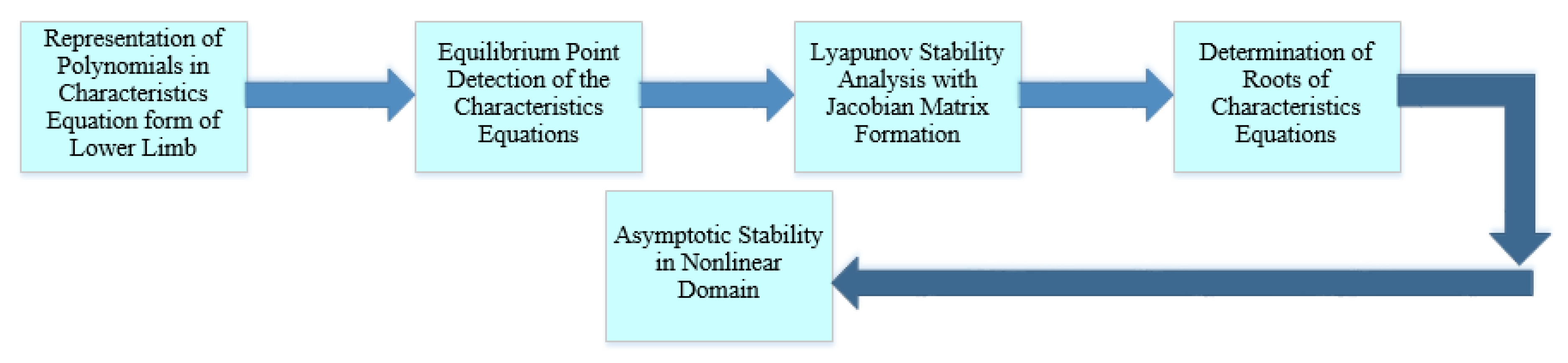
3.2. Workflow of the System Stability Analysis
The workflow of the analysis for lower limb system [40,41] stability with respect to linear and nonlinear systems is shown in Figure 4, Figure 5 and Figure 6, respectively.
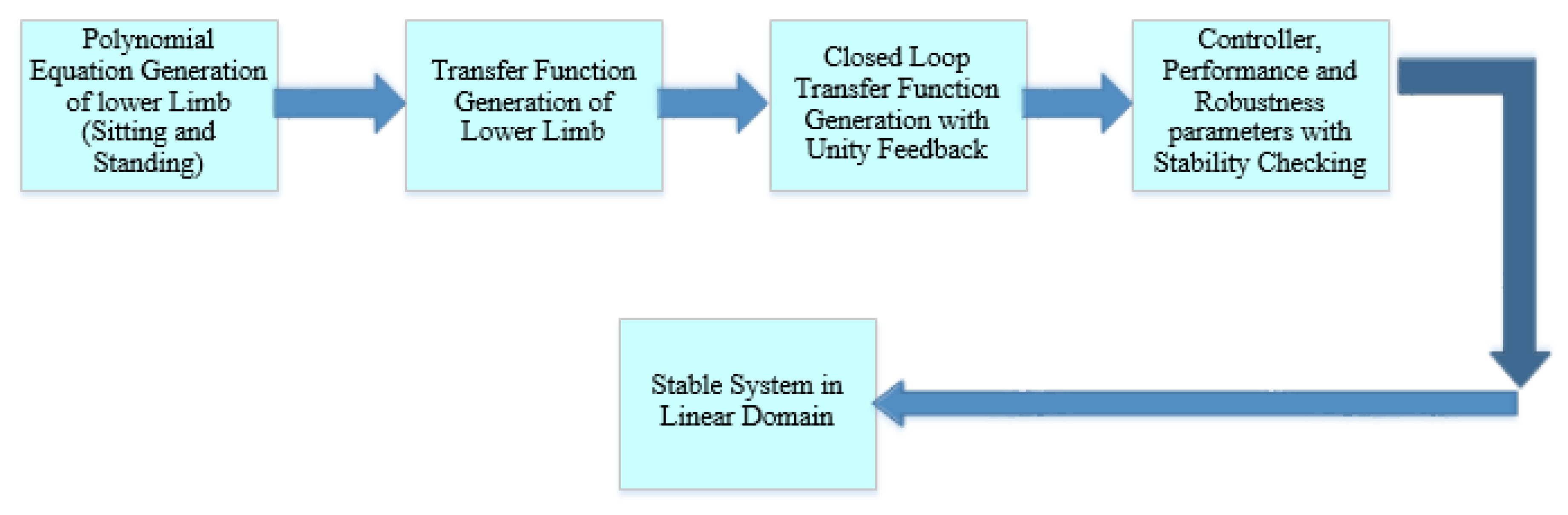
The polynomial equations generated from two different postures of the lower limb, such as sitting and standing, are considered as the primary conditions of the artificial system stability analysis. The transfer function is generated from the polynomials to achieve the mathematical model [42] of the mentioned system. The closed loop transfer function is generated with unity feedback to gather information about the controller, performance and robustness parameters of the system, which shows stability as shown in Figure 4.
The characteristics equation is generated from the polynomials of the system at two different positions of the lower limb. The roots are determined using a computational technique. In the nonlinear domain, using Eigen vectors and the generated matrix, the phase portrait analysis has been incorporated. The system shows asymptotic stability in the nonlinear domain for both the roots of the characteristics equation as shown in Figure 5. For better and stronger decision making on the stability of the system, the Lyapunov stability [43] analysis method has been performed with the equilibrium point detection. This method also shows asymptotic stability where the system is stable and roots are in a complex domain as shown in Figure 6.
4. Results and Discussions
In this present research work, a 3 DoF lower limb has been analyzed for the artificial electro-mechanical system development. The conditions of movement of the human body such as sitting and standing are the main concern in this discussion. Non applicability of the superposition and homogeneity property gives a greater emphasis on the analysis and design of the control systems in the nonlinear domain [15]. The controllability and observability [44] cannot be determined simply based on rank tests. The concept of system stability [45] and checking using Phase portrait and Lyapunov stability [17] has been incorporated to make it a complete evaluation. Polynomials for the two positions of the lower limb (sitting and standing) as shown in Figure 7 and Figure 8 are presented below in Equations (23) and (24), respectively [5]:
See Appendix A.
See Appendix A.
From Equations (23) and (24), the open loop transfer function is obtained, as given below in the Equation (25):
The output graphical presentation of the step response of the open loop transfer function of the system has been shown in the Figure 9.
The closed loop transfer function is given below in Equation (26) derived from Equation (25):
The output graphical presentation of the closed loop transfer function of the system has been shown in Figure 10. The PID (Proportional-Integral-Derivative) controller has been used to tune the closed loop transfer function of the lower limb system. The controller parameters of the closed loop transfer function of the system are shown in Table 1 and the performance and robustness parameters of the closed loop transfer function of the system are shown in Table 2. It is seen that the system is underdamped in Figure 10. The status related to the stability analysis of the mentioned system is prominent from the graphical presentation in Figure 10. The red line is representing the lower limb closed loop transfer function presented in Equation (26) in this paper. Comparing the reference signal represented through the blue line in Figure 10 and the lower limb system output presented in Equation (26), it is observed that the red line, the lower limb system output signal, has reached the stable condition with respect to the blue line at the settling point of the graph. The representations of the red and the blue lines are shown in the legends in Figure 10.
In Figure 10, Table 1 and Table 2 are representing the tuned graphical analysis of the lower limb transfer function presented in Equation (26), using the traditional PID controller. The output performance is not very satisfactory here. So, an advanced controller, the “Control System Designer”, is preferred in order to show the better-tuned output presented in Figure 11 of the lower limb transfer function.
Therefore, the decision making regarding the system stability is possible observing the whole performance of the advanced controller output. In Table 3, the related characteristic parameters are shown. This is clearly shown in that the peak value and the settling time is reduced to a certain level.
Modern technology requires advanced control laws to meet the design specifications for humanoid limb design, thus highlighting the position of nonlinear control systems with recent advancements in the artificial lower limb design. The application area in system design and analysis means that many technologies are developed based on this advanced nonlinear control system stability analysis method. The non-linear system stability analysis is processed as discussed below.
The generated matrix from Equations (23) and (24) is as given below:
Then
where, .
Suppose
Now,
is called the characteristic equation of the matrix A. Since the matrix is singular, .
Therefore,
The roots of the equation are .
Therefore, the two roots are .
For from matrix X, the obtained value is given below:
Suppose, .
Now solving for ,
Using the Gauss elimination method, the obtained simplified equation is
Or,
For from matrix X, obtained value is given below:
Now solving for ,
Using the Gauss elimination method, the obtained simplified equation is
Or,
Now from Equation (27) and using the roots .
The Eigen vectors are given by
This output shows asymptotic stability because for Eigen vectors
the first phase plot is going outward or away from the origin of the plane and the second phase plot is coming towards the origin of the plane as shown in Figure 12. These conditions of phase portrait plot proves an asymptotic stability. The phase plot lines are presented through red lines in Figure 12.
The theory of Lyapunov stability is a standard theory and one of the most important mathematical tools in the analysis of non-linear systems. Now, for further stability checking, the Lyapunov stability method is strongly recommended for nonlinear systems. The followed steps are given below for stability checking:
- Step 1: Representation of polynomials in characteristics equation form.
- Step 2: Determination of the equilibrium point of the system.
- Step 3: Generation of Jacobian matrix to implement in the characteristics equation.
- Step 4: Determination of roots from the characteristics equation.
- Step 5: Verifying the stability conditions from the roots.
- Step 6: Declaration of Asymptotic stability condition.
Now the process of Lyapunov stability method analysis is as shown below:
Let
From Equation (23) it can be written as
From Equation (24) it can be written as
After applying a derivative process in the Equations (36) and (37) respectively, the obtained Equations are as given below:
Now, putting in values from Equation (35), the obtained Equations are as given below:
After applying the derivative process again in the Equations (40) and (41) respectively, the obtained Equations are as given below:
or it can be written as
Now, to find the equilibrium point, it is similar as or it can be written as
Therefore, the equilibrium point is at (0, 0) from Equations (43) and (44).
Now, the Jacobian matrix can be formed using the formula as given below in the Equation (45):
Since, where,
Or,
Or,
Therefore, the roots are .
The abovementioned system has roots containing real and imaginary parts. Therefore, the system can be declared as asymptotically stable. The system performance efficiency is checked through this method.
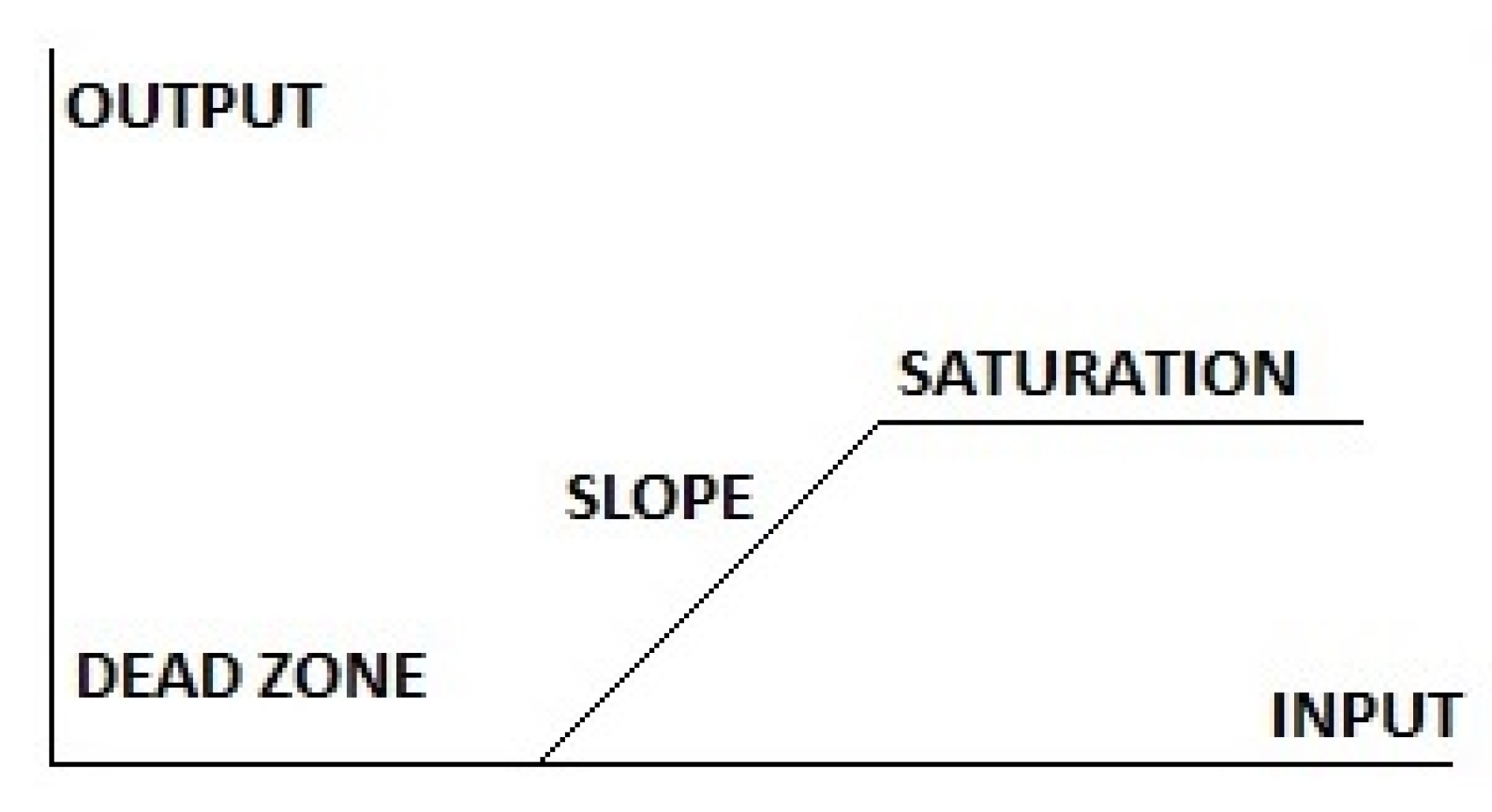
This method is involved to ensure stability of the electro-mechanical system in the field of behavioral quality improvement of the designed artificial model. According to the above results shown through the mathematical models, the nonlinearity nature present in the lower limb system is a dead zone combined with a saturation condition. Figure 13 represents the lower limb system characteristics of overall nonlinearity.
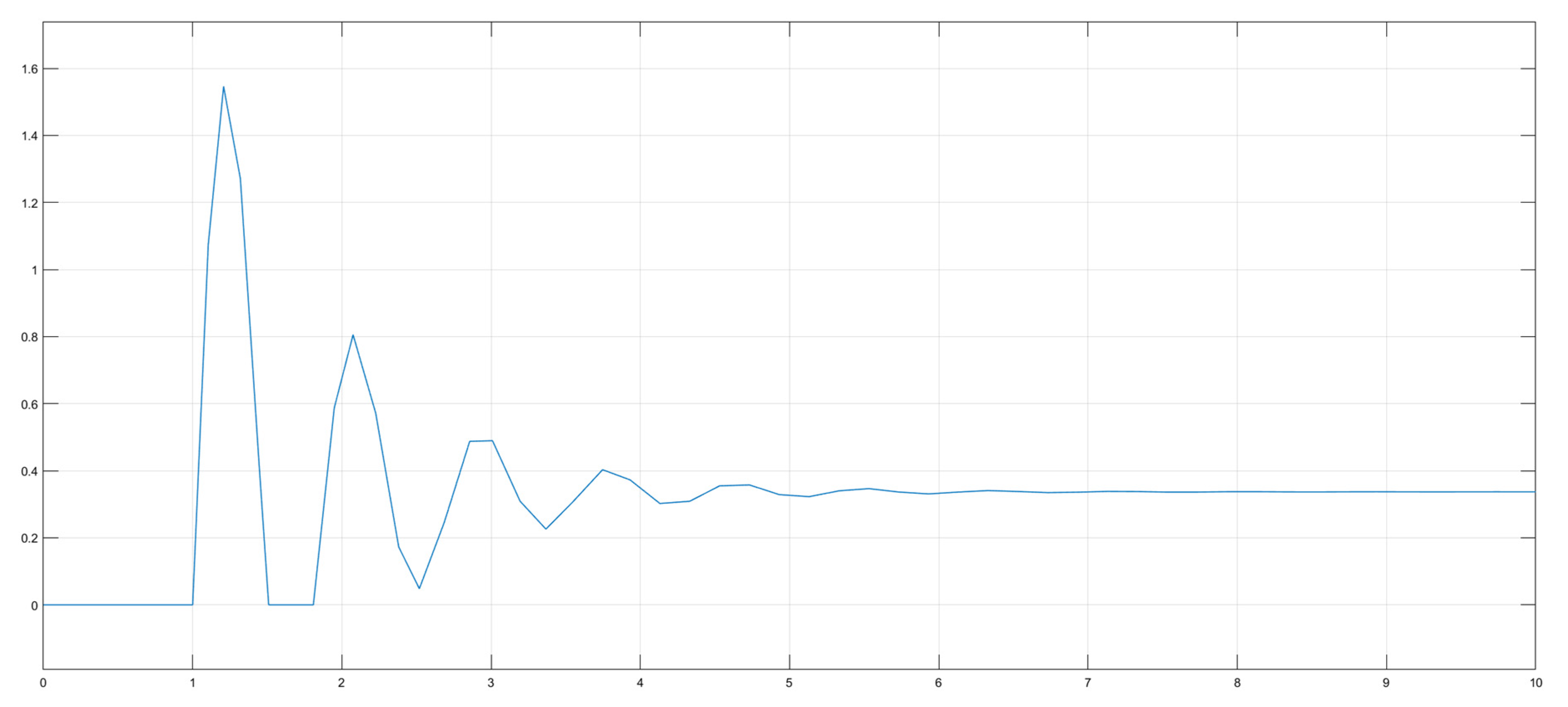
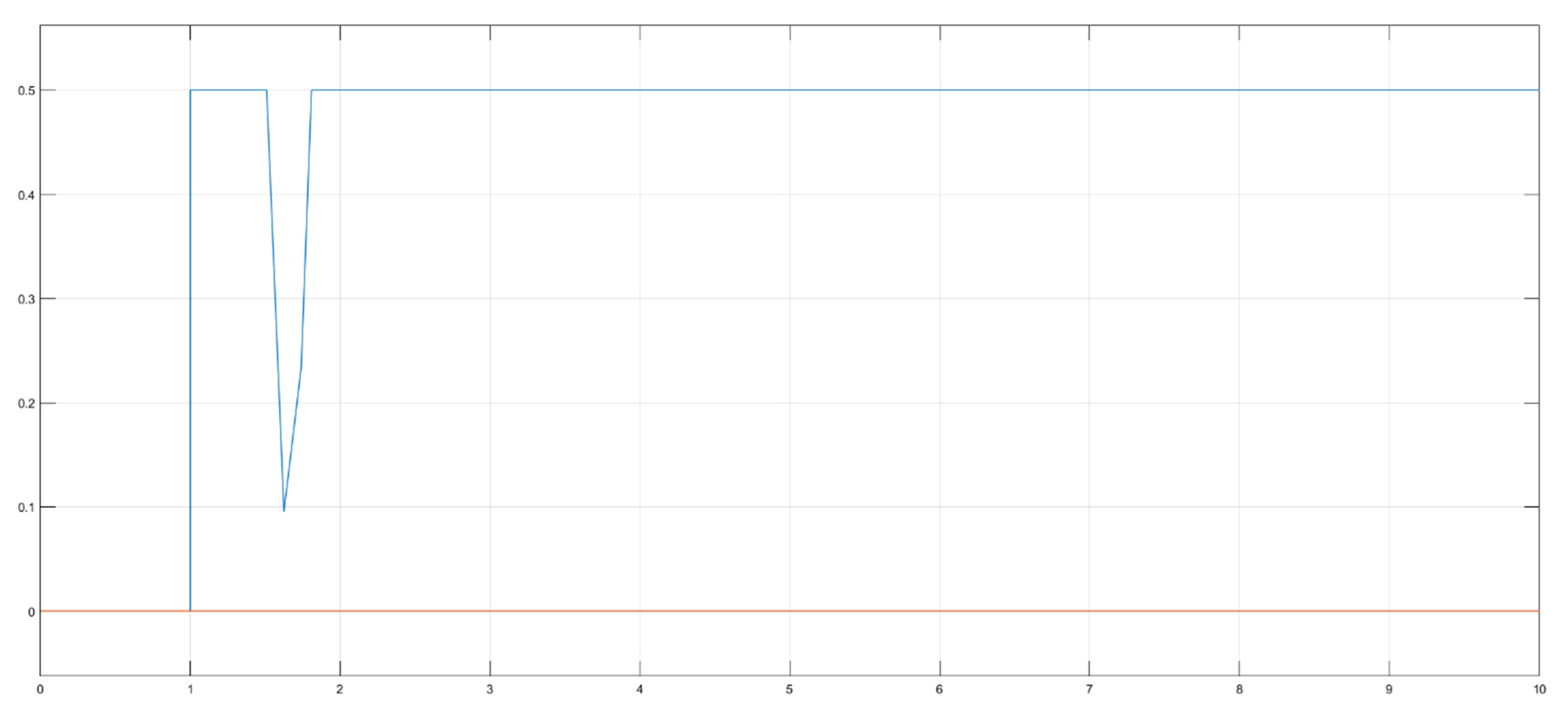
The nonlinear simulation of the lower limb system mentioned in Equation (26) is simulated using the dead zone and saturation functions to show satisfactory output in this paper for the overall simulation of the system. The graphical presentations are presented in Figure 14 and Figure 15, respectively.
The graphical scenario depicts the lower limb system performance regarding nonlinearity. In Figure 14, initially the signal has started to show the activities but after a certain time it has reached the dead zone or the “no action” condition. In Figure 15, initially the signal has started to show output but after a certain period it has reached to saturation condition, being stable at a fixed level. These dead zone and saturation conditions are the specified nonlinear characteristics of the lower limb function only.
The artificial limb design needs to be developed on the basis of knowledge-based system development. This process demands some expertise in the domain of the embedded system. This also requires the intelligent incorporation of an input–output database for the trained functional implementation of humanoid movement with an artificial lower extremity. Modern approaches for nonlinear control systems can be represented as an intelligent control. Various methods can be utilized to develop an automated system using neural networks, machine learning, and fuzzy logic, etc.
5. Conclusions
The nonlinear control systems have gained a challenging position in the technological development of the biomedical application field. In this recent work, the forward dynamics of the robotic system with the DoF concept has been explained using the Euler-Lagrange method. The idea of the mathematical model representation has been demonstrated with the polynomial equation generation from the experimental setup of the lower limb model. The comparative analysis has been incorporated for the system performance analysis using the traditional PID controller and an advanced control system designer. In future, there are lots of opportunities to use a more advanced application of controllers. The system performance stability is checked in two ways. It is found to be asymptotically stable using phase portrait analysis and the most important Lyapunov stability method. The lower limb shows nonlinear behavior. The system remains in the dead zone initially and after a certain period it starts operating. Then it reaches to the saturation level. The overall nonlinear behavior of the lower limb system has been shown here. The role of the describing function is the most important factor to determine the system nature selection. In future, the control system simulation approach can be implemented to get a more informative system identification view of the artificial system design.
Author Contributions
S.D.: Conceptualization, methodology, software, validation, formal analysis, investigation, resources, data curation, writing—original draft preparation, writing—review and editing, visualization, supervision, project administration, funding acquisition. D.N.: Methodology, supervision, review, formal analysis. B.N.: Conceptualization, methodology, supervision, review, formal analysis, project administration, funding acquisition. B.S.: Methodology, review, formal analysis, investigation, visualization, funding acquisition. All authors have read and agreed to the published version of the manuscript.
Funding
This research received no external funding.
Acknowledgments
The authors of the paper are grateful for the support of Indian Institute of Information Technology Kalyani.
Conflicts of Interest
The authors declare no conflict of interest.
Appendix A
In the paper, S. Das, D. Nandi, B. Neogi, “Lower Limb Movement Analysis for Exoskeleton Design”, IEEE TENSYMP 2019, IEEE Region 10 Symposium, the polynomials and are mentioned. These polynomials have been generated for two different positions of the subject such as sitting and standing. From the polynomials, the transfer functional approach is incorporated in this research work for the nonlinearity analysis of the lower limb model.
References
- Dong, S.; Yuan, Z.; Zhang, F. A Simplified Method for Dynamic Equation of Robot in Generalized Coordinate System. In Journal of Physics: Conference Series; IOP Publishing: Bristol, UK, 2019; Volume 1345. [Google Scholar]
- Lynch, K.M.; Park, F.C. Modern Robotics: Mechanics, Planning, and Control; Cambridge University Press: Cambridge, UK, 2017; Chapter 8.1; ISBN 9781107156302. [Google Scholar]
- Al-Shuka, H.; Corves, B.; Zhu, W.-H. Dynamics of Biped Robots during a Complete Gait Cycle: Euler-Lagrange vs. Newton-Euler Formulations; hal-01926090; School of Control Science and Engineering, Shandong University: Jinan, China, 2019. [Google Scholar]
- Zielke, W. A nonlinear system of Euler–Lagrange equations. Reduction to the Korteweg–de Vries equation and periodic solutions. J. Math. Phys. 1975, 16, 1573–1579. [Google Scholar] [CrossRef]
- Das, S.; Das, D.N.; Neogi, B. Lower Limb Movement Analysis for Exoskeleton Design. In Proceedings of the IEEE TENSYMP 2019, IEEE Region 10 Symposium; Symposium Theme: Technological Innovation for Humanity, Kolkata, India, 7–9 June 2019. [Google Scholar]
- Aguiar, A.P. Nonlinear Systems; IST-DEEC PhD Course; Institute for Systems and Robotics: Lisboa, Portugal, 2011. [Google Scholar]
- Wang, L.; Chen, C.; Dong, W.; Wang, L.; Chen, C.; Dong, W.; Du, Z.; Shen, Y.; Zhao, G. Locomotion Stability Analysis of Lower Extremity Augmentation Device. J Bionic Eng. 2009, 16, 99–114. [Google Scholar] [CrossRef]
- Bouzaouache, H.; Braiek, N.B. On the stability analysis of nonlinear systems using polynomial Lyapunov functions. Math. Comput. Simul. 2008, 76, 316–329. [Google Scholar] [CrossRef]
- Chen, G. Stability of Nonlinear Systems. In Encyclopedia of RF and Microwave Engineering; Wiley: New York, NY, USA, 2004; pp. 4881–4896. [Google Scholar]
- Rodríguez-Licea, M.-A.; Perez-Pinal, F.-J.; Nuñez-Pérez, J.-C.; Sandoval-Ibarra, Y. On the n-Dimensional Phase Portraits. Appl. Sci. 2019, 9, 872. [Google Scholar] [CrossRef] [Green Version]
- Hooshmandi, K.; Bayat, F.; Jahed-Motlagh, M.R.; Jalali, A.A. Stability analysis and design of nonlinear sampled-data systems under aperiodic samplings. Int. J. Robust Nonlinear Control 2018, 10, 2679–2699. [Google Scholar] [CrossRef]
- Behera, L. Nonlinear System Analysis—Lyapunov Based Approach; Intelligent Control Lecture Series; CRC Press: Boca Raton, FL, USA, 2003. [Google Scholar]
- Saheya, B.; Chen, G.Q.; Sui, Y.K.; Wu, C.Y. A new Newton-like method for solving nonlinear equations. SpringerPlus 2016, 5, 1269. [Google Scholar] [CrossRef] [Green Version]
- Gyztopoulus, E.P. Stability Criteria for a class of nonlinear systems. Inf. Control 1963, 6, 276–296. [Google Scholar]
- Ajayi, M.O. Modelling and Control of Actuated Lower Limb Exoskeletons: A Mathematical Application Using Central Pattern Generators and Nonlinear Feedback Control Techniques; HAL archives; Tshwane University of Technology: Pretoria, South Africa, 2016. [Google Scholar]
- Liu, Z.; Huang, D.; Xing, Y.; Zhang, C.; Wu, Z.; Ji, X. New Trends in Nonlinear Control Systems and Applications. Abstr. Appl. Anal. 2015, 2015. [Google Scholar] [CrossRef] [Green Version]
- Packard, A.; Poola, K.; Horowitz, R. Jacobian Linearizations, equilibrium points. In Dynamic Systems and Feedback; University of California: Berkeley, CA, USA, 2002. [Google Scholar]
- Yunping, L.; Lipeng, W.; Ping, M.; Kai, H. Stability Analysis of Bipedal Robots Using the Concept of Lyapunov Exponents. Math. Probl. Eng. 2003, 2013, 546520. [Google Scholar] [CrossRef]
- Ku, Y.H.; Chen, C.F. A new method for evaluating the describing function of hysteresis-type nonlinearities. J. Frankl. Inst. 1962, 273, 226–241. [Google Scholar] [CrossRef]
- Úředníček, Z. Describing functions and prediction of limit cycles. WSEAS Trans. Syst. Control 2018, 13, 432–446. [Google Scholar]
- Crooijmans, M.T.M.; Brouwers, H.J.H.; Van Campen, A.D.; De Kraker, A. Limit Cycle Predictions of a Nonlinear Journal-Bearing System. ASME J. Eng. Ind. 1990, 112, 168–171. [Google Scholar] [CrossRef]
- Aracil, J.; Gordillo, F. Describing function method for stability analysis of PD and PI fuzzy controllers. Fuzzy Sets Syst. 2004, 143, 233–249. [Google Scholar] [CrossRef]
- Özyapıcı, A.; Sensoy, Z.B.; Karanfiller, T. Effective Root-Finding Methods for Nonlinear Equations Based on Multiplicative Calculi. J. Math. 2016, 2016, 8174610. [Google Scholar] [CrossRef]
- Adamu, M.Y.; Ogenyi, P.; Tahir, A.G. Analytical solutions of nonlinear oscillator with coordinate-dependent mass and Euler–Lagrange equation using the parameterized homotopy perturbation method. J. Low Freq. Noise Vib. Act. Control 2019, 38, 1028–1035. [Google Scholar] [CrossRef] [Green Version]
- Shi, D.; Zhang, W.; Zhang, W.; Ding, X. A Review on Lower Limb Rehabilitation Exoskeleton Robots. Chin. J. Mech. Eng. 2019, 32, 74. [Google Scholar] [CrossRef] [Green Version]
- Kaze, A.D.; Maas, S.; Arnoux, P.-J.; Wolf, C.; Pape, D. A finite element model of the lower limb during stance phase of gait cycle including the muscle forces. Biomed. Eng. 2017, 16, 138. [Google Scholar]
- Thota, S.; Srivastav, V.K. Quadratically convergent algorithm for computing real root of non-linear transcendental equations. BMC Res. Notes 2018, 11, 909. [Google Scholar] [CrossRef] [Green Version]
- Sande, H.V.; Henrotte, F.; Hameyer, K. The Newton-Raphson method for solving non-linear and anisotropic time-harmonic problems. In COMPEL—The International Journal for Computation and Mathematics in Electrical and Electronic Engineering; Emerald Group Publishing Limited: Bingley, UK, 2004; Volume 23, pp. 950–958. [Google Scholar]
- Yin, L.; Sun, D.; Mei, Q.; Gu, Y.; Baker, J.; Feng, N. The Kinematics and Kinetics Analysis of the Lower Extremity in the Landing Phase of a Stop-jump Task. Open Biomed. Eng. J. 2015, 9, 103–107. [Google Scholar] [CrossRef] [Green Version]
- Tucan, P.; Vaida, C.; Carbone, G.; Pisla, A.; Puskas, F.; Gherman, B.; Pisla, D. A kinematic model and dynamic simulation of a parallel robotic structure for lower limb rehabilitation. In Advances in Mechanism and Machine Science; Uhl, T., Ed.; Springer: Cham, Switzerland, 2019; Volume 73. [Google Scholar]
- Tayyab, M.; Sarkar, B.; Ullah, M. Sustainable Lot Size in a Multistage Lean-Green Manufacturing Process under Uncertainty. Mathematics 2019, 7, 20. [Google Scholar] [CrossRef] [Green Version]
- Dey, B.K.; Sarkar, B.; Pareek, S. A Two-Echelon Supply Chain Management with Setup Time and Cost Reduction, Quality Improvement and Variable Production Rate. Mathematics 2019, 7, 328. [Google Scholar] [CrossRef] [Green Version]
- Dey, B.K.; Pareek, S.; Tayyab, M.; Sarkar, B. Autonomation policy to control work-in-process inventory in a smart production system. Int. J. Prod. Res. 2020, 1–13. [Google Scholar] [CrossRef]
- Sarkar, B.; Mahapatra, A.S. Periodic review fuzzy inventory model with variable lead time and fuzzy demand. Int. Trans. Oper. Res. 2017, 24, 1197–1227. [Google Scholar] [CrossRef]
- Sarkar, B. Mathematical and analytical approach for the management of defective items in a multi-stage production system. J. Clean. Prod. 2019, 218, 896–919. [Google Scholar] [CrossRef]
- Sarkar, B.; Prasad Mondal, S.; Hur, S.; Ahmadian, A.; Salahshour, S.; Guchhait, R.; Waqas Iqbal, M. Solution and Interpretation of Neutrosophic Homogeneous Difference Equation. RAIRO-Oper. Res. 2019, 53, 1649–1674. [Google Scholar] [CrossRef] [Green Version]
- Samanta, S.; Sarkar, B. Generalized fuzzy Euler graphs and generalized fuzzy Hamiltonian graphs. J. Intell. Fuzzy Syst. 2018, 35, 3413–3419. [Google Scholar] [CrossRef]
- Jemai, J.; Sarkar, B. Optimum Design of a Transportation Scheme for Healthcare Supply Chain Management: The effect of energy consumption. Energies 2019, 12, 2789. [Google Scholar] [CrossRef] [Green Version]
- Neogi, B.; Barui, S.; Das, S.; Paul, S.; Ghosh, J.; Ghosh, J. Tuning and transfer functional modelling of a prosthetic arm. J. Comput. Methods Sci. Eng. 2019, 19, 243–256. [Google Scholar] [CrossRef]
- Das, S.; Paul, S.; Ojha, S.K.; Neogi, B.; Nazarov, A.; Ghosh, J.; Ghosh, J. On Design and Implementation of an Artificial Lower Limb. Int. J. Sens. Wirel. Commun. Control 2018, 8, 100–108. [Google Scholar] [CrossRef]
- Paul, S.; Ojha, S.K.; Barui, S.; Ghosh, S.; Ghosh, M.; Neogi, B.; Ganguly, A. Technical Advancement on Various Bio-signal Controlled Arm- A review. J. Mech. Contin. Math. Sci. 2018, 13, 95–111. [Google Scholar] [CrossRef]
- Neogi, B.; Ghosal, S.; Mukherjee, S.; Das, A.; Tibarewala, D.N. Simulation Techniques and Prosthetic Approach towards Biologically Efficient Artificial Sense Organs- An Overview. arXiv 2011, arXiv:1111.1684. [Google Scholar]
- Neogi, B.; Ghosal, S.; Sarkar, S. Analysis and Control Towards Limb Prosthesis for Paraplegic and Fatigued Conditions by Introducing Lyapunov and Sample Data Domain Aspects. Int. Rev. Autom. Control 2012, 5, 548–552. [Google Scholar]
- Paul, S.; Barui, S.; Chakraborty, P.; Jana, D.R.; Neogi, B.; Nazarov, A. Mechanical Prosthetic Arm Adaptive I-PD Control Model Using MIT Rule Towards Global Stability. J. Mech. Contin. Math. Sci. 2018, 13, 43–55. [Google Scholar] [CrossRef]
- Banerjee, S.; Bhattacharjee, S.; Nag, A.; Bhattacharyya, S.; Neogi, B. Discrete Domain Analysis of Dexterous Hand Model by Simulation Aspect. Procedia Technol. 2012, 4, 878–882. [Google Scholar] [CrossRef] [Green Version]
Figure 1.
Block diagram of the forward dynamics of a nonlinear system.

Figure 2.
Functional diagram of the forward dynamics model.

Figure 3.
Pictorial representation of the artificial Lower limb with joints and links.

Figure 4.
Workflow of the system stability analysis in the linear domain.

Figure 5.
Workflow of the phase portrait stability Analysis in the nonlinear domain.

Figure 6.
Workflow of the Lyapunov stability analysis in the nonlinear domain.

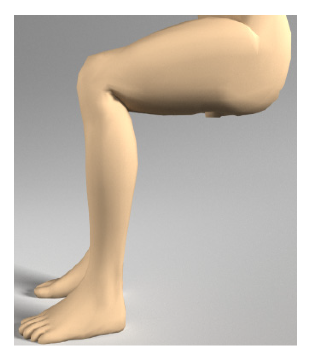
Figure 7.
Sitting condition of normal Human Lower Limb.

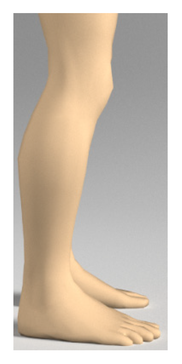
Figure 8.
Standing condition of normal Human Lower Limb.

Figure 9.
Graphical representation of the step response of the open loop transfer function of the system.
Figure 9.
Graphical representation of the step response of the open loop transfer function of the system.

Figure 10.
Graphical representation of the closed loop transfer function of the system.

Figure 11.
Graphical representation of the closed loop transfer function of the system using an advanced control system designer.
Figure 11.
Graphical representation of the closed loop transfer function of the system using an advanced control system designer.

Figure 12.
Phase portrait plot of nonlinear system.

Figure 13.
Representation of the characteristics of overall nonlinearity in the lower limb system.

Figure 14.
Graphical representation of the characteristics of the dead zone of the lower limb system.
Figure 14.
Graphical representation of the characteristics of the dead zone of the lower limb system.

Figure 15.
Graphical representation of the characteristics of the saturation of the lower limb system.
Figure 15.
Graphical representation of the characteristics of the saturation of the lower limb system.


Table 1.
Controller parameters of the closed loop transfer function of the system.
| Proportional Constant (kp) | Integral Constant (ki) | Derivative Constant (kd) | Stability Status |
|---|---|---|---|
| 0.92214 | 2.8732 | 0 | Stable |
Table 2.
Performance and Robustness parameters of the closed loop transfer function of the system.
| Rise Time (s) | Settling Time (s) | Overshoot (%) | Peak (s) | Stability Status |
|---|---|---|---|---|
| 0.626 | 7.77 | 10.3 | 1.1 | Stable |
Table 3.
Performance and robustness parameters of the closed loop transfer function of the system.
| Rise Time (s) | Settling Time (s) | Peak Amplitude (s) | Stability Status |
|---|---|---|---|
| 0.00191 | 5.05 | 0.965 | Stable |
Publisher’s Note: MDPI stays neutral with regard to jurisdictional claims in published maps and institutional affiliations. |
© 2020 by the authors. Licensee MDPI, Basel, Switzerland. This article is an open access article distributed under the terms and conditions of the Creative Commons Attribution (CC BY) license (http://creativecommons.org/licenses/by/4.0/).
Share and Cite
MDPI and ACS Style
Das, S.; Nandi, D.; Neogi, B.; Sarkar, B. Nonlinear System Stability and Behavioral Analysis for Effective Implementation of Artificial Lower Limb. Symmetry 2020, 12, 1727. https://doi.org/10.3390/sym12101727
AMA Style
Das S, Nandi D, Neogi B, Sarkar B. Nonlinear System Stability and Behavioral Analysis for Effective Implementation of Artificial Lower Limb. Symmetry. 2020; 12(10):1727. https://doi.org/10.3390/sym12101727
Chicago/Turabian StyleDas, Susmita, Dalia Nandi, Biswarup Neogi, and Biswajit Sarkar. 2020. "Nonlinear System Stability and Behavioral Analysis for Effective Implementation of Artificial Lower Limb" Symmetry 12, no. 10: 1727. https://doi.org/10.3390/sym12101727
Note that from the first issue of 2016, this journal uses article numbers instead of page numbers. See further details here.