A Qualitative Tool Condition Monitoring Framework Using Convolution Neural Network and Transfer Learning


Laboratory of Intelligent Manufacturing, Design and Automation (LIMDA), Department of Mechanical Engineering University of Alberta, Edmonton, AB T6G1H9, Canada
*
Author to whom correspondence should be addressed.
Appl. Sci. 2020, 10(20), 7298; https://doi.org/10.3390/app10207298
Submission received: 26 September 2020
/
Revised: 15 October 2020
/
Accepted: 16 October 2020
/
Published: 19 October 2020
(This article belongs to the Special Issue Machining Dynamics and Parameters Process Optimization)
Abstract
:Tool condition monitoring is one of the classical problems of manufacturing that is yet to see a solution that can be implementable in machine shops around the world. In tool condition monitoring, we are mostly trying to define a tool change policy. This tool change policy would identify a tool that produces a non-conforming part. When the non-conforming part producing tool is identified, it could be changed, and a proactive approach to machining quality that saves resources invested in non-conforming parts would be possible. The existing studies highlight three barriers that need to be addressed before a tool condition monitoring solution can be implemented to carry out tool change decision-making autonomously and independently in machine shops around the world. First, these systems are not flexible enough to include different quality requirements of the machine shops. The existing studies only consider one quality aspect (for example, surface finish), which is difficult to generalize across the different quality requirements like concentricity or burrs on edges commonly seen in machine shops. Second, the studies try to quantify the tool condition, while the question that matters is whether the tool produces a conforming or a non-conforming part. Third, the qualitative answer to whether the tool produces a conforming or a non-conforming part requires a large amount of data to train the predictive models. The proposed model addresses these three barriers using the concepts of computer vision, a convolution neural network (CNN), and transfer learning (TL) to teach the machines how a conforming component-producing tool looks and how a non-conforming component-producing tool looks.
1. Introduction
The last decade has been the decade of the fourth industrial revolution (Industry 4.0) for manufacturing around the world using smart systems and technology. Industry 4.0 uses the concepts of machine learning and big data to reduce wastage of time and resources and make the production process more efficient [1,2]. The concepts of Industry 4.0 require machines that are smart and autonomous [3], and this presents an excellent opportunity for the development of machine learning algorithms that improve operations and help in the reduction of waste.
Smart systems are essential for the implementation of Industry 4.0 in machine shops, but what is the definition of a smart machine in the context of machining quality control? There is no clear definition proposed in past studies. A smarter machine in the context of machining quality control can be envisioned as a machine with the intelligence to understand and implement the quality requirements. This machine only produces the parts that meet the design requirements (i.e., conforming parts) and detects the changes in machining parameters or environmental factors. These changes in environmental factors might result in the manufacturing of parts that do not meet the design requirements (i.e., non-conforming parts). In other words, the machine has the intelligence to predict whether the machine will produce a conforming or a non-conforming part based on the environmental inputs.
In a mass manufacturing facility, the environmental factors like type of machine used, jigs, and fixtures in which the machining is taking place are reasonably stable, and these are changed only when the production lines are repurposed to produce different components. Given the stable environmental factors, the quality of the machining largely depends on the consumables like cutting tools, coolant oils, and others used by these machining processes [4,5]. If the consumables are used for too long, they contribute to the production of non-conforming parts, and if the consumables are underutilized, they add to the overheads and wastage [6]. The process of defining the limits for an overused and an underused tool can be termed a tool change policy (TCP) and is illustrated in Section 4. In an intelligent tool condition monitoring (TCM) system, the definition and implementation of a TCP should be carried out autonomously and independently.
TCM is one of the classical problems of manufacturing, and it has been extensively studied in the last four decades [7,8]. However, three barriers have been identified by the presented study that challenge the deployment of existing solutions in machine shops around the world. First, the inflexibility of the systems to accommodate different TCPs: tool condition affects different aspects of machining like surface finish [9] and dimensional accuracy [10,11]. For example, a TCP for one tool is when the chatter marks start to appear, while for another tool TCP it is related to a burr on the edge. The existing studies fail to provide flexibility to accommodate different TCPs.
Quantification of tool wear ignores the concept of a TCP and diverts the attention to the quantification of wear on inserts, and this is the second identified challenge for deployment of current TCM systems. The studies try to quantify the wear on inserts in terms of millimeters of flank wear [12,13,14,15]. This quantification provides no information about the usability of the tool. In machine shops around the world, quality management is not seen as a process that directly adds value to the component, and from an economic point this process must be limited to what is absolutely necessary [16]; that is why the manufacturers are interested to know whether components meet the design requirements (a conforming part) or do not meet design requirements (a non-conforming part). One of the examples for this qualitative approach is GO (conforming part)/NO GO (non-conforming part) gauges [17], which are discussed in Section 3. Therefore, the central objective of TCM must also be qualitative so that it recognizes the GO quality tool (tool that produces conforming part) and the NO GO quality tool (tool that produces non-conforming part).
The final barrier identified is the large amount of data and time required to collect and train these systems, which is the most significant barrier in the accommodation of different TCPs. The models have to be retrained for different quality requirements that require changing the parameters learned by the predictive systems. For example, Wu et al. [15] used 5880 images to train a model for the detection of different wear patterns. Considering four cutting edges per insert, the model used 1470 inserts for training. Collecting these extensive data for every machine and TCP is infeasible considering the hundreds of different quality requirements in machine shops around the world.
The proposed system is an integrated solution to the three barriers mentioned above. The system relies on monitoring the wear of cutting tools and classifies the tools as GO/NO GO tools that help the machine operator make the decision on whether the tool can be used for the next machining cycle. The system uses state-of-the-art tool wear classification in the form of a convolution neural network (CNN) and principles of transfer learning (TL). These concepts are discussed in Section 3. The novelty of the system is its ability to correlate the tool condition with machining quality and the accommodation of different quality requirements using a TCP with the requirement of fewer data to achieve the accommodation.
The rest of the research paper is structured as follows. In Section 2, the relevant studies are discussed. Section 3 explains the methodology used in the system, which can be divided into training, offline state, and online state. In Section 4, the case study and the implementation of the proposed system are discussed and the evaluation of the proposed system is performed in Section 5, followed by the suggested future direction of tool condition monitoring. In the final section, the conclusions drawn from the study are discussed.
2. Literature Review
Tool condition monitoring methods are classified into direct and indirect methods [18]; direct methods mostly involve the use of computer vision [14,15], radiation [19], and electrical resistance [20], whereas indirect methods involve online monitoring methods that use vibration [21,22,23], force [22], and temperature and sound [24] signals. Indirect methods are less complicated and can be implemented straightforwardly and monitored in real-time [10], but they are prone to making noise and are less accurate than the direct methods [25]. Real-time monitoring is also not a crippling disadvantage for direct systems as there is enough time in between machining operation and cycles [26] to get the required data without disturbing the sequence of operations of a machine shop. In addition, the unidirectional execution of existing G-code-based systems does not allow for real-time changes in the machining parameters [27,28,29]; therefore, there is no way to integrate the response generated by indirect systems in real-time. Considering direct methods are more accurate systems, the study adopts the direct monitoring methodology.
Vision-based systems are the most popular systems when it comes to direct tool condition monitoring. Vision systems have also improved in recent years and are being used in different facets of machining like collision avoidance [2,30], which also demonstrates the ability of vision systems to detect changes while maintaining distance from the cutting process. Computer vision systems are used to monitor changes in the wear morphologies of an insert. Wear morphology classification has been the subject of many studies in past years; Lanzetta [31] employed vision systems for wear morphology classification using quantitative definitions of different wear patterns. The conventional tool condition monitoring used in machine shops involves the quantitative approach. For autonomous systems, the quantitative approach proves difficult for implementation considering the variety of qualitative parameters that need to be hardcoded into the system to identify a variety of wear morphologies. The hard coding of parameters is also computationally expensive; thus, there is a need for a system that identifies the features of different types of wear. The need for identification of different morphologies is satisfied to an extent using CNN by Wu et al. [15]; this study has inspired the base wear classification model discussed in Section 3.1.
Autonomously detecting damage to the inserts before they are used in machining is one of the essential requirements for making tool monitoring autonomous. Fernandez-Robles et al. [32] developed a vision-based system to detect broken inserts in milling cutters automatically. Sun et al. [14] used image processing and image segmentation techniques to develop a system that could identify built-up edges, fractures, and other insert deformations. These studies used image processing techniques, which require human intervention to develop feature descriptions; this limits the independent implementation of these systems for a variety of wear morphologies. As opposed to image processing techniques, the CNN approach learns to identify the region of interest (ROI) and features descriptions to identify different wear morphologies, and this eliminates the need for the human feature descriptions step needed in other techniques [33]. Considering the utility of autonomous feature extraction, the proposed study uses the CNN approach for tool condition monitoring.
Even though tool condition monitoring is one of the classical problems, there are fewer publications in the context of the correlation of tool condition with the quality of the component. Jain and Lad [34] developed a system that correlates tool condition and production quality. The study also developed a multi-level categorization of the wear using a support vector machine methodology. Jain and Lad [35] explored the relationship between surface finish and tool wear and found the Pearson correlation coefficient between surface finish and tool condition to be significant to establish a strong correlation. The study used a random forest-based fault estimation model to determine the relation between surface finish and tool condition. Grzenda and Bustillo [36], developed a semi-supervised model to predict the surface finish using vibration signals; Fourier transformation was used to transform signals to frequency space, and only the relevant frequency ranges were considered for the study. Wu et al. [15] developed a two-stage system that aimed to determine the type of wear in the first stage and tried to quantify the wear of the insert in a milling cutter. The system used CNN to determine the type of wear, and the wear value was obtained using the relation between image pixel value and actual value and width of the minimum circumscribed rectangle. Dutta et al. [37] used surface texture descriptions to determine tool life using the grey level co-occurrence matrix; the images of the resulting surface finish were captured, and the tool wear was measured using a microscope. García-Ordás et al. [25] used a computer vision system to determine the usefulness of milling cutters. The system used a support vector machine methodology to classify the wear patterns. The system identified the state of the tool with about 90 percent accuracy.
The studies mentioned above correlate tool condition with the specific quality and design requirements like surface finish. As discussed in Section 1, there are a variety of quality and design requirements that are defined by TCP. These different TCPs form the ultimate definition of TCM; considering this, a TCM that is flexible enough to accommodate different TCPs is the need of the hour. Most of the studies are also limited by the materials and tool geometries they have used, and changing any one of the factors means the findings of the studies cannot be used. For the TCM to be autonomous and independent, it must be capable of working with different materials, tool geometries, and tool coating grades. The requirements of flexibility to work with different TCPs and the ability to generalize the system for different working materials, tool geometries, and tool coating grades, form the basis for the development of the proposed system.
3. Qualitative Tool Condition Monitoring System
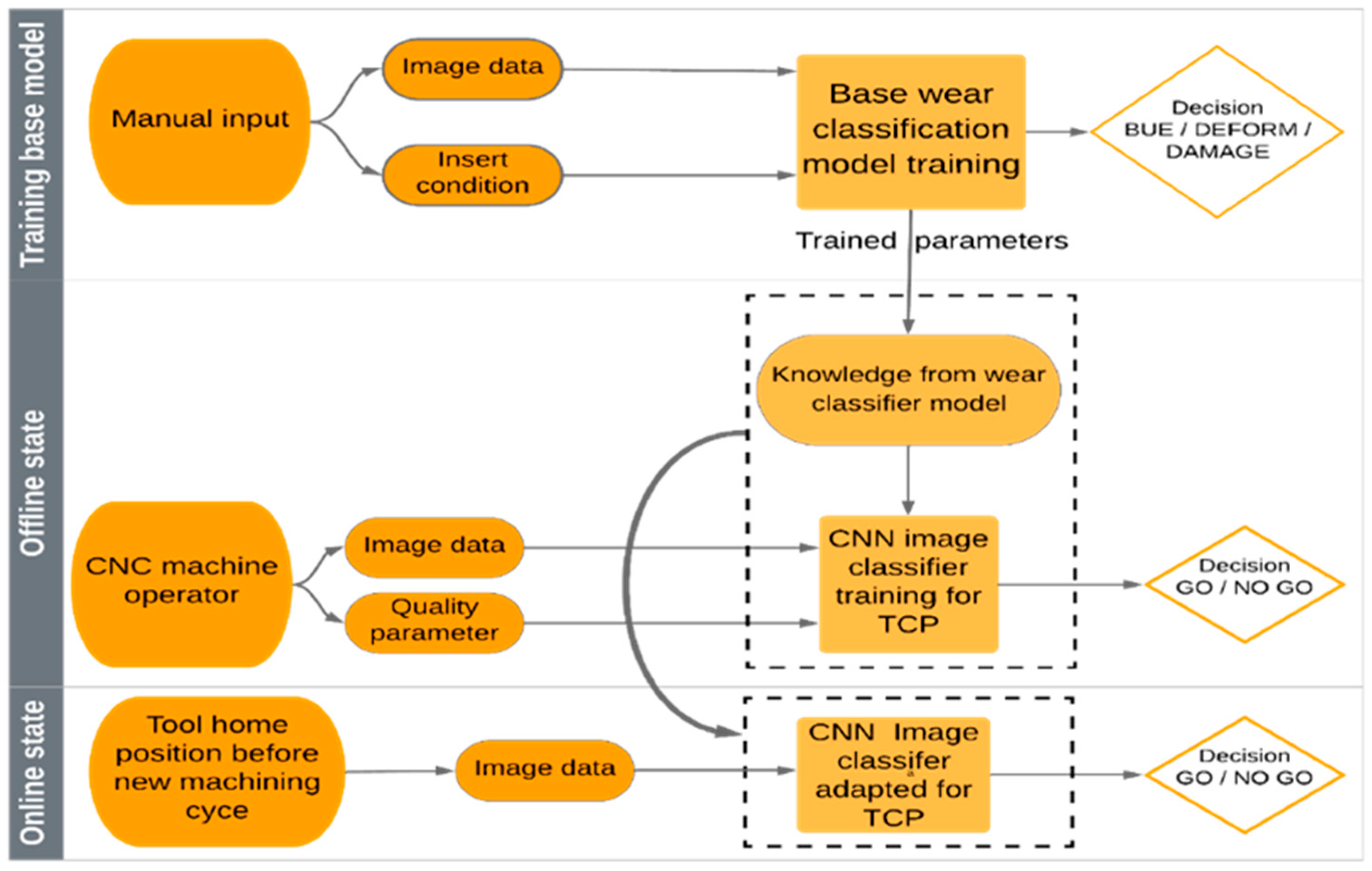
The system is developed to operate in three stages, as shown in Figure 1. The training of the base model is where the architecture of the base model and the central intelligence of the system are developed; this training is done remotely. The architecture and training parameters of the base model are discussed in Section 3.1. The offline state of the system is operational in the machine shops when the production lines are set up. In this state, the system is receiving training to identify the TCP. The knowledge from the base wear classification model is used to expedite this training process using the TL technique discussed in Section 3.2. The output of the system is inspired by the GO/NO GO gauges. The goal of the GO gauge is to accept as many good parts as possible that satisfy the material condition specification, and NO GO gauges are designed to reject all the parts that violate the material condition specification [17]. The GO/NO GO gauge in this system is envisioned as an implementation of a TCP. When a tool of GO quality is detected, the tool is accepted and used for production. When a NO GO quality tool is detected, the operator is asked to change the tool before resuming the production. The GO/NO GO arrangement allows for the flexibility to adapt the system for different TCPs. In the online state of the system discussed in Section 3.3, the system is executing the TCP autonomously after every machining cycle, making sure the tools are in GO condition before they are used, and in this way provides a proactive approach to TCM.
3.1. The Base Wear Classification Model
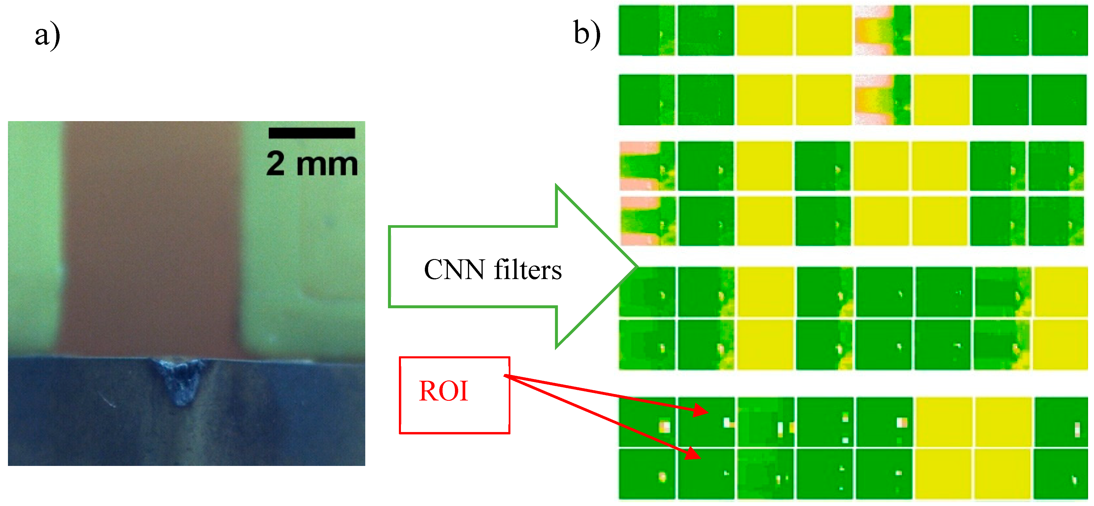
A CNN is one of the most promising approaches to image processing and pattern recognition [33]. CNN layers are part of the architecture; it is standard practice to use convolution layers at the start of the model to develop feature descriptions of the images. These layers are good at narrowing down the ROI and require less computational memory when compared to conventional models. These are the reasons they have seen a wide range of applications in a variety of areas, from hand gesture recognition [38] to disease recognition in plants [39]. One of the other advantages of the convolution layers is their ability to extract features autonomously. Some of these transformations are shown in Figure 2. In Figure 2b, each row is the output of convolution or max pooling layers. It can be seen in the successive layers. The layer transformation and filtering further define the description of the wear features. This step in image processing techniques is done manually, which is the disadvantage of image processing techniques.
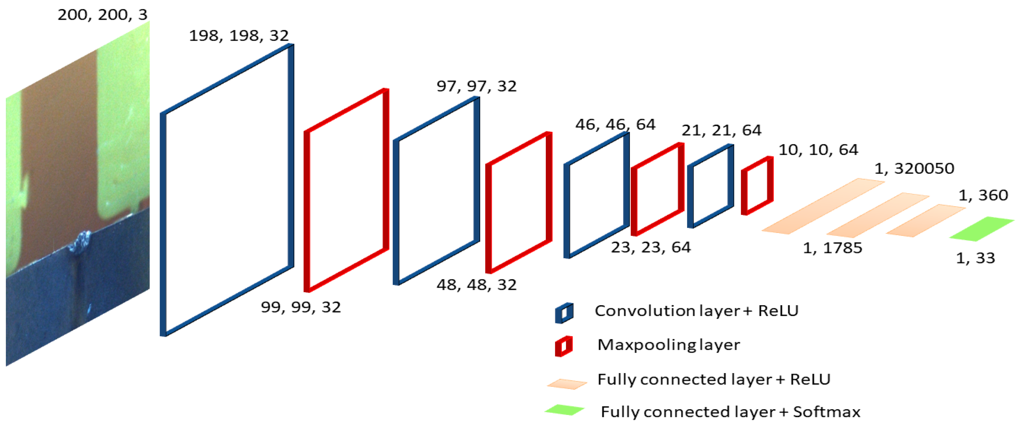
The base model architecture used by the system is shown in Figure 3. The input to this architecture is a 200 × 200 × 3 Red Green Blue image (RGB). The convolution layers have sparse interaction with the input of the previous layer [40]. For the convolution layer, a 3 × 3 kernel is used with 32 filters in the first and second convolution layers. For the last two convolution layers, 64 filters are used with a 3 × 3 kernel. A kernel can be imagined as a 3 × 3 window sliding over 200 × 200 in the step of a one-pixel slide. This concept helps in the detection of small meaningful features and also reduces the parameters to be stored and computed [40]. The output of the convolution layer is then fed to the pooling layer, in the case of the developed model, it is the max pooling layer, where the kernel reports the maximum value of the kernel size input. This layer helps in making the model more robust in response to small translations to the inputs [40]. This is summarized in Equation (1), where A is the corresponding pixel value in row i and column j, and this equation is valid for the 2 × 2 kernel used for max pooling layers.
Max pooling layer
Oi,j = max {Ai,j, Ai+1,j, Ai,j+1, Ai+1,j+1}
The output of the last max pooling layer is then flattened to a 1 × vector, which forms the input to the fully connected layers (FCLs) for further processing, where is the number of inputs to the neural network. The number of inputs also determines the width of the FCLs of the network.
FCLs are the basic type of neural network where each input interacts with each output of the previous layer [40], the different layers in the network are modeled as different functions, which are the function of the previous layer. In the proposed base model shown in Figure 3, we have four FCL layers, which can be written as f(1), f(2), f(3), and f(4). Using the chain concept we can rewrite these functions as f(xi) = f(4)(f(3)(f(2)(f(1)(xn)))) [40], where xn is the data from the convolution layers. The objective of the neural network is to best estimate f(xn; θ) to function f * (xn), where f * (xn) is the ideal (real-world relation) function that maps the inputs from the convolution layer to their classes of wear and θ is a free parameter adjusted to optimize the best estimation of an ideal function [40].
The architecture in Figure 3 uses a rectified linear unit (ReLU) activation function in the intermediate layers, which is a common practice for CNNs to improve the training speed [39]. The ReLU returns zero for half of its domain and is the input for the other half of the domain that is zero for inactive nodes and is the node output for active nodes, which helps make the gradients of the loss function large and constant [40]. The ReLU is used in all the layers except the output layer in the proposed model shown in Figure 3. The ReLU is summarized in Equation (2), where z is the output of the node.
The softmax activation function was used in the last layer of the base model architecture, which is also common in multiclass classification CNNs [39]. Softmax activation usually used in the output layers of the neural networks gives the probability distribution over n possible values. It ensures that the prediction of z belonging to a class for n different classes is between 0 and 1, and the sum of probabilities is equal to 1 [40]. This is summarized in Equation (3), where zp is the output of the node for the p class.
The loss of a model can be defined as a function that quantifies the performance of the system [33]; the study uses categorical cross-entropy as the loss function. ADAM, which is a stochastic optimizer that is computationally efficient and combines the advantages of RMSProp and AdaGrad [41], was used to optimize the weights of the base model. This facilitated faster convergence to an optimal solution [40]. The parameters used in ADAM were learning rate = 0.001, beta1 = 0.9, and beta2 = 0.999. The algorithm for ADAM implementation can be found in [41].
3.2. CNN Image Classifier Trained for TCP
The base model developed and discussed in Section 3.1 forms the central intelligence for the TCM. The base model helps narrow down the ROI and extract useful features and descriptions of the tool, as shown in Figure 2. This intelligence is developed in the base model and rolled out as a trained network. The offline stage of the system is in the machine shops, where the model has to be repurposed to identify and implement different TCPs. Considering that there are thousands of different TCP unique to each machine shop, retraining a complete network presents a significant data and training time challenge. TL is one of the lifelines to overcome this data and training time challenge.
Given the importance of TL, we now adapt the definitions of TL in [42] for our application. In the proposed system, the knowledge developed during the training of the wear classification model to identify what type of wear pattern or damage the cutting tool has is optimized using TL to differentiate between a good tool that produces conforming parts and a bad tool that produces non-conforming parts. Every classification model has a domain D, which forms the pool for data extraction and a task which, in the case of this study, is classification. Pan and Yang [42] define domain D as consisting of two components: a feature space X and a marginal probability P(X). Task T also consists of two-component Y labels and a predictive function f(.); since neural networks have a large number of trainable parameters they can choose from different functions that best predict the task, which in the case of our study is image classification. Therefore and and considering these definitions we can define source domain and target domain. The source domain is images captured from cutting inserts used in machining (DS), and the task is to identify wear type classification (TS). Similarly, the target domain is images of inserts used in production (DT), and the task is the quality classification (TT).
The images for the base model are drawn for the inserts used in production. Similarly, images used for the target model are also drawn from inserts used in production. Therefore, the methodology is built around the assumption that the images for the source and target model have a similar domain, which is reasonable considering that the images used to train base model wear morphology classification are also used in production in a machine shop. Given the similarity of domains, XS = XS, PS(X) = PT(X), and DS = DT, that is, the feature space and the marginal probability of data distribution for both models are the same.
The tasks of the source and target models are different as the labels are different, therefore TS ≠ TT as YS ≠ YT, as given by Equations (4) and (5). But the predictive function could be similar or different since the neural networks are black-box models. There is no way to know if the same or a different function was used for source and target tasks.
The target task is tied up to the traditional concepts of GO/NO GO gauges discussed at the start of Section 3. GO/NO GO gauges are one of the most popular gauges to evaluate the material conditions in holes and shafts. The tool condition monitoring system developed extends and generalizes this definition of GO/NO GO gauges to other quality requirements. In the target task, the model is retrained to identify a GO part producing tool and NO GO part producing tool. This concept makes the proposed methodology qualitative and gives the model the flexibility to adapt its knowledge across different TCPs. The offline state requires an expert to generate the GO/NO GO labels for the training and adaptation of the task to the TCP.
3.3. CNN Image Classifier Adapted for TCP
The online state of the system works seamlessly without the need for human intervention to identify the tools that produce a NO GO part. The system takes a picture before the machining starts and, based on the training during the offline state, classifies the tool as a useable or unusable tool. There are many tools on the machine, and the quality demand from each tool is different. Therefore, the offline part of the system where the tool condition is associated with GO/NO GO quality of operation has to be performed on each tool during the production setup. This allows the system to run without quality inspection in the online state.
4. Experimental Setup
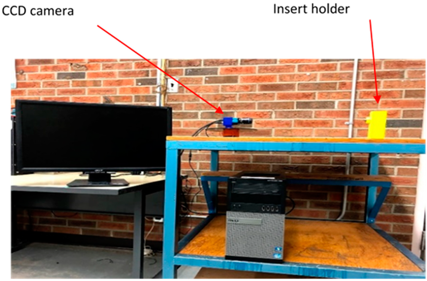
The images of the CNMG 120408/12, TNMG 160408/12, and VNMG 160408 turning inserts used in the turning application are captured using the DFK 33GP006 GigE color camera with TCL 3520 5MP lens. Initially, the top, side, and front views are considered for the classification. A processor with Intel i7 and 16 GB RAM was used to develop the classification model, and the models were implemented using R computer language with the Keras package using a TensorFlow backend. Examples of these pictures can be seen in Table 1. Table 1 shows that the top and side views do not clearly show the type of wear, but the wear is easily distinguishable in the front view images; therefore, only front view images were considered for the classification model. The setup for capturing the images of different views can be seen in Figure 4. The images are captured in standard room lighting without any dedicated light source. As we can see from Figure 2, the background of the insert has no impact on the feature extraction process.
The process started with collecting the front-view images of the inserts for three different categories: 79 images of damaged inserts, 121 images of deformed inserts, and 128 images of abrasive wear inserts were captured. All the pictures were then resized to 200 (width) × 200 (height).
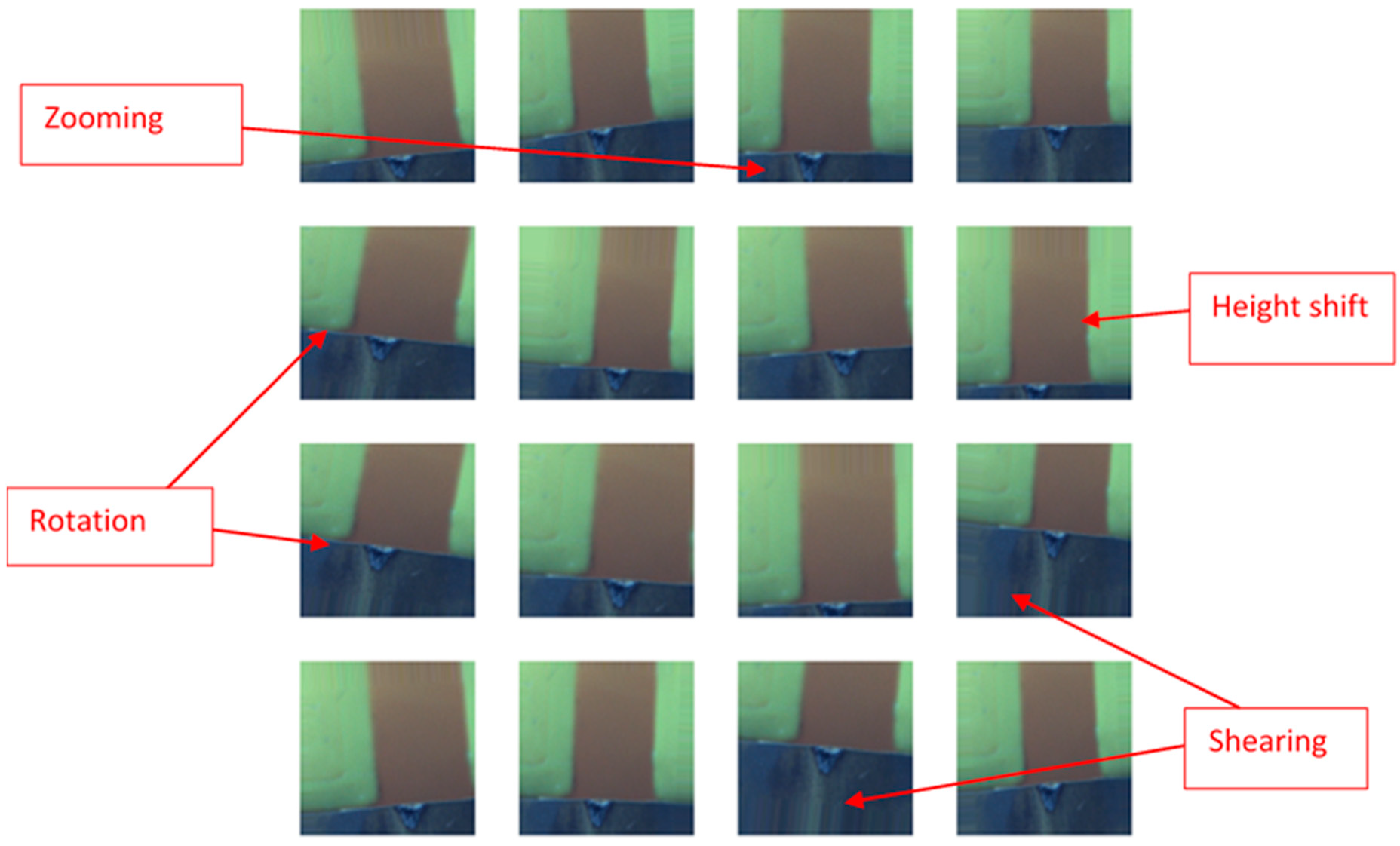
The model must be made robust against variation and transformation. One of the ways to do this is to use data augmentation, where the data are subjected to various transformations such as rotation, flipping, and shearing the images; this helps in improving the generalization error as the model is trained to be invariant to these transformations [40]. The training dataset was subjected to data augmentation, with an allowed rotation range of 10 degrees, width shift range of 20 percent, height shift range of 10 percent, and zooming range of 20 percent. The parameters for augmentation were chosen carefully so as not to alter the wear description of the images, but to accommodate for poor quality images that can be seen when the system is deployed in machine shops. An example of this data augmentation can be seen in Figure 5. It should be noted that the validation images were not subjected to data augmentation.
The augmented data were then fed to the neural networks. The images were first subjected to the image transformations of the convolution and max pooling layers, where the ROI was identified, and useful features were extracted from the images autonomously. The data in the final layers formed the last max pooling layer and formed the input to the densely connected layers. The images were converted to pixel data, and each pixel formed the input to the first FCL; the data were mapped to the labels of the pictures, and the output of the FCL was the prediction of wear type. The base model can now identify the nuanced differences in the cutting insert by identifying if the insert has deformation, normal wear, or damage. The knowledge developed in the base model can now be used to identify the change in quality by retaining the model.
For the target model, the images of inserts are classified into GO/NO GO categories; for this part of the study, only CNMG 120408 turning inserts are used; one of the examples for GO/NO GO can be seen in Table 2. Table 2 also gives an example for different TCPs accessible in machine shops. The objective of the case study with respect to the target model is to prove that the model identifies the nuanced differences in changes in wear morphology and predicts the consequence of using a tool. That is, if the tool produces a GO quality part or NO GO quality part while using lesser images and training time and iterations so that the TCP deployment is fast-tracked.
For this part of the study, inserts that are relatively new and have typical wear patterns are manually classified as GO category inserts, and the inserts that have higher wear levels, as shown in the NO GO part of Table 2, are classified as NO GO category inserts. These images are used to train the target model, and the training images are subjected to similar data augmentation to that shown in Figure 5. The architecture of the target model is shown in Table 3. The parameters learned by the base model are frozen, and only 382 parameters of layers 12 and 13 are optimized for the target model.
5. Results and Discussion
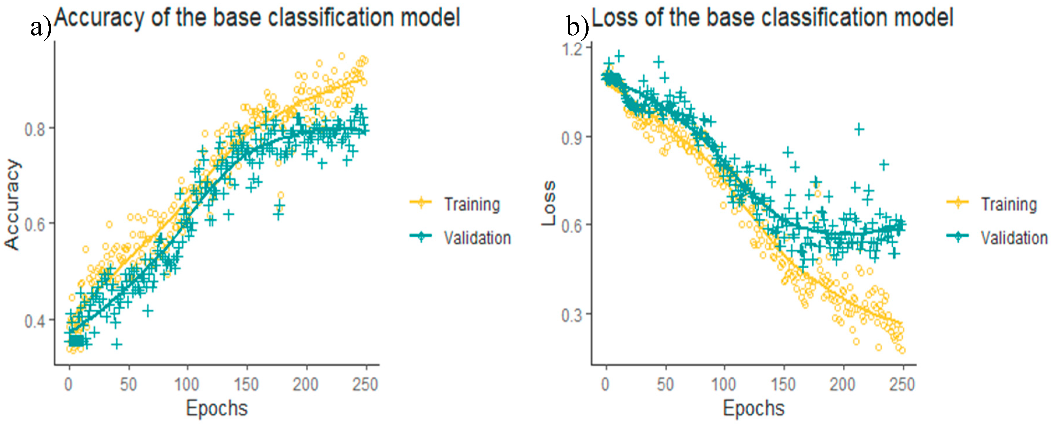
The training of the base model was carried out using 223 images, and 105 images were split from the original dataset for validation; the validation data set consists of approximately 33 percent from each of the damaged, deformation, and abrasive wear categories. Figure 6a gives the accuracy for base model training runs. The validation accuracy stabilized around the 200th epoch, and the validation accuracy is 83.75 percent. Figure 6b presents the loss of over 250 epochs, and the loss is the indication of the magnitude of deviation between prediction and the actual value.
For the second part, the objective is to demonstrate the capability of the system to adapt to the new task of TCP deployment using fewer images and shorter training time. For this, the data are partitioned into three sections: training, validation, and test dataset; various training runs are carried out using a different number of images. The summary of the number of images used for each run is shown in Table 4. All the images in the three sections are different and are not repeated. The images in the test data set can be seen in Figure 7; the GO category images have no wear or have typical wear pattern; these tools produce conforming parts, and the NO GO category have visible wear on the edges; these tools produce non-conforming parts.
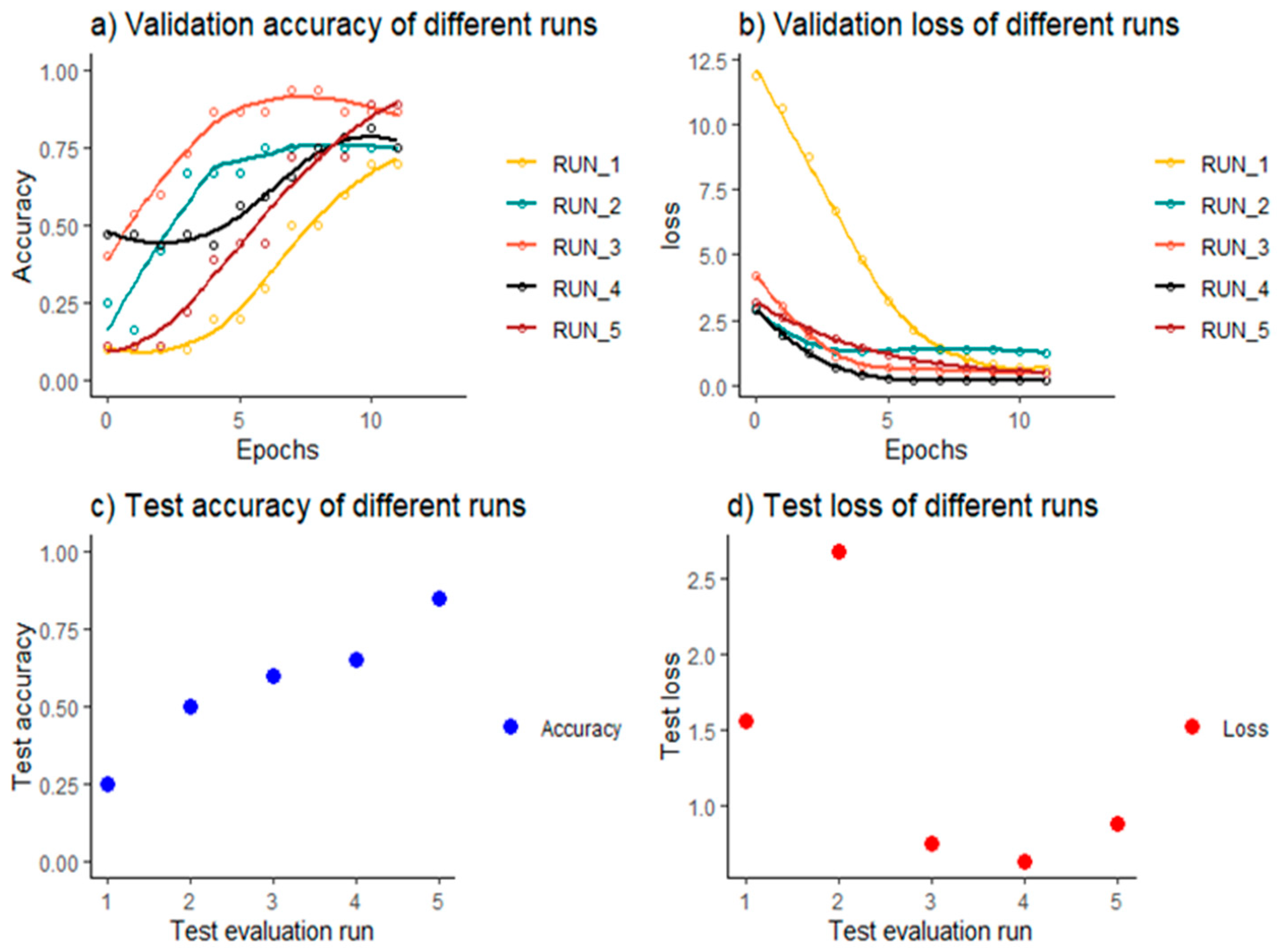
Figure 8 shows the accuracy and loss values for different runs. It can be seen from Figure 8b that the loss value plateaued around the 5th epoch in most of the runs, signifying that the optimization of the parameters requires fewer iterations, which enables the system to accommodate a variety of TCPs and with fewer training requirements. Figure 8c and d show the accuracy and loss of the trained models on the test dataset. It can be seen that the accuracy of the models increases with the number of images used for training the model. Run 4 had a smaller loss value when compared to run 5 but had lower accuracy; this can be attributed to overfitting of data which led to misclassification of the images in the NO GO category test data as GO category images. Run 5 had the best results in terms of accuracy on test data, where 37 images were used in training the model. The accuracy of the test data for run 5 was 85 percent; the confusion matrix for run 5 can be seen in Table 5. The model predicted all NO GO label images correctly and predicted 3 images of GO labels incorrectly.
The final part of the study is the deployment of the system using a graphical user interface (GUI). Figure 9 gives a view of the GUI; the output of the GUI is feedback to the operator. The feedback is NO GO for tools that the target model predicts will produce a non-conforming part, and GO for tools that the model predicts will produce a conforming part. The machine operator is encouraged to replace the tool when the GUI displays NO GO. The prediction is generated within 5 s, facilitating the mass production without interruptions from quality inspections.
The proposed system directs the TCM from a quantitative to a qualitative approach using a TCP. This is the reason the study does not consider quantification of the wear using any measuring system, and this makes the system more flexible to accommodate different quality requirements seen in machine shops around the world. The system uses the feature extraction capabilities of CNN and the ability of these models to learn new features using TL. Future development in the proposed system has three fronts. First, the development of the camera system to be integrated into the machine: the image acquisition in the study was independent of the machine, but the system has demonstrated that the images acquired at a reasonable distance away from the cutting operation can be used and classified by the system. The system uses standard room lighting; there are systems discussed in studies done by Sun et al. [14], which are capable of generating the required light intensity and protecting the camera from cutting oil. Second, improvement of the intelligence and accuracy of the system by integrating more diverse wear images into the base model: since the base model is the central nervous system and target models have similar data distribution, the accuracy of the GO/NO GO model can be improved with fewer iteration requirements, and with a more robust base model. Finally, the proposed system is designed for the turning process: considering that the wear mechanisms in milling are different, there is a need to develop a similar system for milling applications. A similar neural network can be trained with milling insert data to repurpose the framework for a milling application. The CNN architecture is a standard approach when it comes to image recognition and identification-related neural network architectures. The area of deep learning also continues to evolve; therefore, there is a need to keep an eye out for new techniques that can improve the training time and accuracy of the system.
6. Conclusions
The proposed study redirects tool condition monitoring from tool wear quantification to the objective of providing a more proactive qualitative approach to quality management that saves the resources used in the production of non-conforming parts. A tool change policy is employed to detect these changes in quality indicators and change the tools when they occur. Given the different quality requirements, there are a variety of tool change policies. Therefore, tool condition monitoring that is flexible enough to adapt to different tool change policies is developed. The developed systems can adapt to a new tool change policy requiring as few as 37 images and 12 training iterations using concepts of transfer learning and convolution neural networks. The study also developed a qualitative approach to tool condition monitoring, since the issue that is more important than quantifying the wear on a cutting tool is whether the tool produces a conforming or a non-conforming part. This is captured in the system by extending the concept of GO/NO GO gauges to different quality requirements through tool conditions. The tools that are predicted to produce a conforming part are categorized as GO tools, while non-conforming part producing tools are classified as NO GO tools. The developed system can identify the GO/NO GO quality tool with 85 percent accuracy. Lastly, a graphical user interface is also developed to give feedback to machine operators about the usability of the tools. The system is designed to operate in between machining cycles, checking the usability of every tool before they are used. The system only takes a few seconds to determine the usability of the tools. This concept helps in making the proposed methodology an in-process tool condition monitoring system.
Author Contributions
Conceptualization, H.M.; methodology, H.M. and M.A.S.; software, H.M.; validation, H.M. and M.A.S.; formal analysis, H.M.; investigation, H.M.; resources, R.A.; data curation, H.M.; writing—original draft preparation, H.M.; writing—review and editing, R.A.; visualization, H.M.; supervision, R.A.; project administration, R.A.; funding acquisition, R.A. All authors have read and agreed to the published version of the manuscript.
Funding
We express our gratitude to the Minister of Economic Development, Trade, and Tourism for funding this project through Major Innovation Funds. The authors also would like to acknowledge the NSERC (Grant Nos. NSERC RGPIN-2017-04516 and NSERC CRDPJ 537378-18) for further funding this project.
Acknowledgments
We express our gratitude to the Minister of Economic Development, Trade, and Tourism for funding this project through Major Innovation Funds. The authors also would like to acknowledge the NSERC (Grant Nos. NSERC RGPIN-2017-04516 and NSERC CRDPJ 537378-18) for further funding this project.
Conflicts of Interest
The authors declare no conflict of interest.
References
- Albers, A.; Gladysz, B.; Pinner, T.; Butenko, V.; Stürmlinger, T. Procedure for Defining the System of Objectives in the Initial Phase of an Industry 4.0 Project Focusing on Intelligent Quality Control Systems. Procedia CIRP 2016, 52, 262–267. [Google Scholar] [CrossRef] [Green Version]
- Ahmad, R.; Tichadou, S.; Hascoet, J.Y. Generation of safe and intelligent tool-paths for multi-axis machine-tools in a dynamic 2D virtual environment. Int. J. Comput. Integr. Manuf. 2016, 29, 982–995. [Google Scholar] [CrossRef]
- Lee, J.; Bagheri, B.; Kao, H.A. A Cyber-Physical Systems architecture for Industry 4.0-based manufacturing systems. Manuf. Lett. 2015, 3, 18–23. [Google Scholar] [CrossRef]
- Wang, G.F.; Yang, Y.W.; Zhang, Y.C.; Xie, Q.L. Vibration sensor based tool condition monitoring using ν support vector machine and locality preserving projection. Sens. Actuators A Phys. 2014, 209, 24–32. [Google Scholar] [CrossRef]
- Khorasani, A.M.; Gibson, I.; Goldberg, M.; Doeven, E.H.; Littlefair, G. Investigation on the effect of cutting fluid pressure on surface quality measurement in high speed thread milling of brass alloy (C3600) and aluminium alloy (5083). Meas. J. Int. Meas. Confed. 2016, 82, 55–63. [Google Scholar] [CrossRef]
- Pratama, M.; Dimla, E.; Lai, C.Y.; Lughofer, E. Metacognitive learning approach for online tool condition monitoring. J. Intell. Manuf. 2019, 30, 1717–1737. [Google Scholar] [CrossRef] [Green Version]
- Ghani, J.A.; Rizal, M.; Nuawi, M.Z.; Ghazali, M.J.; Haron, C.H.C. Monitoring online cutting tool wear using low-cost technique and user-friendly GUI. Wear 2011, 271, 2619–2624. [Google Scholar] [CrossRef]
- Jinpeng, S.; Shaowei, L.; Ahmad, R.; Jiaojiao, G.; Ming, L. Tribological behaviour of TiB2-HfC ceramic tool material under dry sliding condition. Ceram. Int. 2020, 46, 20320–20327. [Google Scholar] [CrossRef]
- Jinpeng, S.; Jiaojiao, G.; Ahmad, R.; Ming, L. Cutting performances of TiCN–HfC and TiCN–HfC–WC ceramic tools in dry turning hardened AISI H13. Adv. Appl. Ceram. 2020. [Google Scholar] [CrossRef]
- Teti, R.; Jemielniak, K.; O’Donnell, G.; Dornfeld, D. Advanced monitoring of machining operations. CIRP Ann. Manuf. Technol. 2010, 59, 717–739. [Google Scholar] [CrossRef] [Green Version]
- Kilundu, B.; Dehombreux, P.; Chiementin, X. Tool wear monitoring by machine learning techniques and singular spectrum analysis. Mech. Syst. Signal Process. 2011, 25, 400–415. [Google Scholar] [CrossRef]
- Mikołajczyk, T.; Nowicki, K.; Bustillo, A.; Pimenov, D.Y. Predicting tool life in turning operations using neural networks and image processing. Mech. Syst. Signal Process. 2018, 104, 503–513. [Google Scholar] [CrossRef]
- D’Addona, D.M.; Teti, R. Image data processing via neural networks for tool wear prediction. Procedia CIRP 2013, 12, 252–257. [Google Scholar] [CrossRef]
- Sun, W.H.; Yeh, S.S. Using the machine vision method to develop an on-machine insert condition monitoring system for computer numerical control turning machine tools. Materials 2018, 11, 1977. [Google Scholar] [CrossRef] [Green Version]
- Wu, X.; Liu, Y.; Zhou, X.; Mou, A. Automatic identification of tool wear based on convolutional neural network in face milling process. Sensors 2019, 19, 3817. [Google Scholar] [CrossRef] [Green Version]
- Orzan, I.A.; Buzatu, C. CONAT 2016 International Congress of Automotive and Transport Engineering; Springer: Berlin/Heidelberg, Germany, 2017. [Google Scholar] [CrossRef]
- Meadows, J.D. Measurement of Geometric Tolerances in Manufacturing. In Manufacturing Engineering and Materials Processing; CRC Press: New York, NY, USA, 1998; pp. 1–5. ISBN 9780429165504. [Google Scholar]
- Azouzi, R.; Guillot, M. On-line prediction of surface finish and dimensional deviation in turning using neural network based sensor fusion. Int. J. Mach. Tools Manuf. 1997, 37, 1201–1217. [Google Scholar] [CrossRef]
- Jetley, S.K. Applications of surface activation in metal cutting. In Proceedings of the Twenty-Fifth International Machine Tool Design and Research Conference, Birmingham, UK, 22–24 April 1985. [Google Scholar]
- Wilkinson, A.J. Constriction-resistance concept applied to wear measurement of metal-cutting tools. Proc. Inst. Electr. Eng. 1971, 118, 381. [Google Scholar] [CrossRef]
- Wu, T.Y.; Lei, K.W. Prediction of surface roughness in milling process using vibration signal analysis and artificial neural network. Int. J. Adv. Manuf. Technol. 2019, 102, 305–314. [Google Scholar] [CrossRef]
- Kene, A.P.; Choudhury, S.K. Analytical modeling of tool health monitoring system using multiple sensor data fusion approach in hard machining. Meas. J. Int. Meas. Confed. 2019, 145, 118–129. [Google Scholar] [CrossRef]
- Khorasani, A.M.; Yazdi, M.R.S. Development of a dynamic surface roughness monitoring system based on artificial neural networks (ANN) in milling operation. Int. J. Adv. Manuf. Technol. 2017, 93, 141–151. [Google Scholar] [CrossRef]
- da Silva, R.H.; da Silva, M.B.; Hassui, A. A probabilistic neural network applied in monitoring tool wear in the end milling operation via acoustic emission and cutting power signals. Mach. Sci. Technol. 2016, 20, 386–405. [Google Scholar] [CrossRef]
- García-Ordás, M.T.; Alegre-Gutiérrez, E.; Alaiz-Rodríguez, R.; González-Castro, V. Tool wear monitoring using an online, automatic and low cost system based on local texture. Mech. Syst. Signal Process. 2018, 112, 98–112. [Google Scholar] [CrossRef]
- Siddhpura, A.; Paurobally, R. A review of flank wear prediction methods for tool condition monitoring in a turning process. Int. J. Adv. Manuf. Technol. 2013, 65, 371–393. [Google Scholar] [CrossRef]
- Ahmad, R.; Tichadou, S.; Hascoet, J.Y. 3D safe and intelligent trajectory generation for multi-axis machine tools using machine vision. Int. J. Comput. Integr. Manuf. 2013, 26, 365–385. [Google Scholar] [CrossRef]
- Ahmad, R.; Tichadou, S. Integration of vision based image processing for multi-axis CNC machine tool safe and efficient trajectory generation and collision avoidance. J. Mach. Eng. 2010, 10, 53–65. [Google Scholar]
- Ahmad, R.; Tichadou, S.; Hascoet, J.Y. A knowledge-based intelligent decision system for production planning. Int. J. Adv. Manuf. Technol. 2017, 89, 1717–1729. [Google Scholar] [CrossRef]
- Ahmad, R.; Tichadou, S.; Hascoet, J.Y. New computer vision based Snakes and Ladders algorithm for the safe trajectory of two axis CNC machines. CAD Comput. Aided Des. 2012, 44, 355–366. [Google Scholar] [CrossRef]
- Lanzetta, M. A new flexible high-resolution vision sensor for tool condition monitoring. J. Mater. Process. Technol. 2001, 119, 73–82. [Google Scholar] [CrossRef]
- Fernández-Robles, L.; Azzopardi, G.; Alegre, E.; Petkov, N. Machine-vision-based identification of broken inserts in edge profile milling heads. Robot. Comput. Integr. Manuf. 2017, 44, 276–283. [Google Scholar] [CrossRef]
- Traore, B.B.; Kamsu-Foguem, B.; Tangara, F. Deep convolution neural network for image recognition. Ecol. Inform. 2018, 48, 257–268. [Google Scholar] [CrossRef] [Green Version]
- Jain, A.K.; Lad, B.K. A novel integrated tool condition monitoring system. J. Intell. Manuf. 2017, 30, 1423–1436. [Google Scholar] [CrossRef]
- Jain, A.K.; Lad, B.K. Quality control based tool condition monitoring. In Proceedings of the Annual Conference of the Prognostics and Health Management Society, Coronado, CA, USA, 1 January 2015; pp. 418–427. [Google Scholar]
- Grzenda, M.; Bustillo, A. Semi-supervised roughness prediction with partly unlabeled vibration data streams. J. Intell. Manuf. 2019, 30, 933–945. [Google Scholar] [CrossRef]
- Dutta, S.; Datta, A.; Das Chakladar, N.; Pal, S.K.; Mukhopadhyay, S.; Sen, R. Detection of tool condition from the turned surface images using an accurate grey level co-occurrence technique. Precis. Eng. 2012, 36, 458–466. [Google Scholar] [CrossRef]
- Lin, H.I.; Hsu, M.H.; Chen, W.K. Human hand gesture recognition using a convolution neural network. IEEE Int. Conf. Autom. Sci. Eng. 2014, 2014, 1038–1043. [Google Scholar] [CrossRef]
- Sun, X.; Mu, S.; Xu, Y.; Cao, Z.; Su, T. Image Recognition of Tea Leaf Diseases Based on Convolutional Neural Network. In Proceedings of the 2018 International Conference on Security, Pattern Analysis, and Cybernetics (SPAC), Jinan, China, 14–17 December 2018; pp. 304–309. [Google Scholar] [CrossRef] [Green Version]
- Goodfellow, I.; Bengio, Y.; Courville, A. Deep Learning; MIT Press: Cambridge, MA, USA, 2016. [Google Scholar]
- Kingma, D.P.; Ba, J.L. Adam: A method for Stochastic Optimization. ICLR 2015, 2015, 1–15. [Google Scholar]
- Pan, S.J.; Yang, Q. A survey on transfer learning. IEEE Trans. Knowl. Data Eng. 2010, 22, 1345–1359. [Google Scholar] [CrossRef]
Figure 1.
Overview of the system architecture.

Figure 2.
Convolution layer image transformation: (a) original image of wear; (b) convolution transformation for region of interest (ROI) and feature extraction.
Figure 2.
Convolution layer image transformation: (a) original image of wear; (b) convolution transformation for region of interest (ROI) and feature extraction.

Figure 3.
Base convolution neural network (CNN) architecture for insert wear classification.

Figure 4.
Image capturing station.

Figure 5.
Examples of rotation, shearing, height shift, and zooming data augmentation applied to training images.
Figure 5.
Examples of rotation, shearing, height shift, and zooming data augmentation applied to training images.

Figure 6.
(a) Accuracy of the base model. (b) Loss convergence graph of the base model.

Figure 7.
Test image data: (a) GO images; (b) NO GO images.

Figure 8.
Results for target model training run on validation and test datasets.

Figure 9.
Graphical user interface (GUI) for quality management system.


Table 1.
Wear patterns and different views.
| Wear Pattern | Top View | Side View | Front View |
|---|---|---|---|
| Damaged |  |  |  |
| Deformation |  |  |  |
| Abrasive |  |  |  |
Table 2.
GO, NO GO, and examples of different tool change policies used in machine shops around the world.
Table 2.
GO, NO GO, and examples of different tool change policies used in machine shops around the world.
| NO GO | GO | GO | GO | GO | Quality |
|---|---|---|---|---|---|
 |  |  |  |  | Insert wear image |
 |  |  |  |  | Surface finish |
 |  |  |  |  | Burrs on edge |
 |  |  |  |  | Chatter marks |
 |  |  |  |  | Feed marks |
Table 3.
Target model architecture.
| Layer Type | Input Shape | Output Shape | Filter Size | Trainable Parameters | |
|---|---|---|---|---|---|
| 0 | Input layer | 200,200,3 | 200,200,3 | 0 | |
| 1 | Convolution layer | 200,200,3 | 198,198,32 | 3,3,32 | 0 |
| 2 | Max pooling layer | 198,198,32 | 99,99,32 | 2,2,32 | 0 |
| 3 | Convolution layer | 99,99,32 | 97,97,32 | 3,3,32 | 0 |
| 4 | Max pooling layer | 97,97,32 | 48,48,32 | 2,2,32 | 0 |
| 5 | Convolution layer | 48,48,32 | 46,46,64 | 3,3,64 | 0 |
| 6 | Max pooling layer | 46,46,64 | 23,23,64 | 2,2,64 | 0 |
| 7 | Convolution layer | 23,23,64 | 21,21,64 | 3,3,64 | 0 |
| 8 | Max pooling layer | 21,21,64 | 10,10,64 | 2,2,64 | 0 |
| 9 | flatten (Flatten) | 10,10,64 | 6400,1 | 0 | 0 |
| 10 | Dense layer | 6400,1 | 50,1 | 0 | 0 |
| 11 | Dense layer | 50,1 | 35,1 | 0 | 0 |
| 12 | Dense layer | 35,1 | 10,1 | 0 | 360 |
| 13 | Dense layer | 10,1 | 2,1 | 0 | 22 |
Table 4.
Training, validation, and test data split for different runs.
| RUN | Training Pictures | Validation Pictures | Test Pictures |
|---|---|---|---|
| 1 | 13 | 10 | 20 |
| 2 | 18 | 12 | 20 |
| 3 | 23 | 16 | 20 |
| 4 | 27 | 18 | 20 |
| 5 | 37 | 26 | 20 |
Table 5.
Confusion matrix for run 5.
| Prediction | GO | NO GO | |
|---|---|---|---|
| Actual | |||
| GO | 7 | 0 | |
| NO GO | 3 | 10 | |
Publisher’s Note: MDPI stays neutral with regard to jurisdictional claims in published maps and institutional affiliations. |
© 2020 by the authors. Licensee MDPI, Basel, Switzerland. This article is an open access article distributed under the terms and conditions of the Creative Commons Attribution (CC BY) license (http://creativecommons.org/licenses/by/4.0/).
Share and Cite
MDPI and ACS Style
Mamledesai, H.; Soriano, M.A.; Ahmad, R. A Qualitative Tool Condition Monitoring Framework Using Convolution Neural Network and Transfer Learning. Appl. Sci. 2020, 10, 7298. https://doi.org/10.3390/app10207298
AMA Style
Mamledesai H, Soriano MA, Ahmad R. A Qualitative Tool Condition Monitoring Framework Using Convolution Neural Network and Transfer Learning. Applied Sciences. 2020; 10(20):7298. https://doi.org/10.3390/app10207298
Chicago/Turabian StyleMamledesai, Harshavardhan, Mario A. Soriano, and Rafiq Ahmad. 2020. "A Qualitative Tool Condition Monitoring Framework Using Convolution Neural Network and Transfer Learning" Applied Sciences 10, no. 20: 7298. https://doi.org/10.3390/app10207298
Note that from the first issue of 2016, this journal uses article numbers instead of page numbers. See further details here.