Day Ahead Bidding of a Load Aggregator Considering Residential Consumers Demand Response Uncertainty Modeling

State Key Laboratory of Advanced Electromagnetic Engineering and Technology, Huazhong University of Science and Technology, Wuhan 430074, China
*
Author to whom correspondence should be addressed.
Appl. Sci. 2020, 10(20), 7310; https://doi.org/10.3390/app10207310
Submission received: 16 September 2020
/
Revised: 13 October 2020
/
Accepted: 14 October 2020
/
Published: 19 October 2020
(This article belongs to the Special Issue Resilient and Sustainable Distributed Energy Systems)
Abstract
:As the electricity consumption and controllability of residential consumers are gradually increasing, demand response (DR) potentials of residential consumers are increasing among the demand side resources. Since the electricity consumption level of individual households is low, residents’ flexible load resources can participate in demand side bidding through the integration of load aggregator (LA). However, there is uncertainty in residential consumers’ participation in DR. The LA has to face the risk that residents may refuse to participate in DR. In addition, demand side competition mechanism requires the LA to formulate reasonable bidding strategies to obtain the maximum profit. Accordingly, this paper focuses on how the LA formulate the optimal bidding strategy considering the uncertainty of residents’ participation in DR. Firstly, the physical models of flexible loads are established to evaluate the ideal DR potential. On this basis, to quantify the uncertainty of the residential consumers, this paper uses a fuzzy system to construct a model to evaluate the residents’ willingness to participate in DR. Then, based on the queuing method, a bidding decision-making model considering the uncertainty is constructed to maximize the LA’s income. Finally, based on a case simulation of a residential community, the results show that compared with the conventional bidding strategy, the optimal bidding model considering the residents’ willingness can reduce the response cost of the LA and increase the LA’s income.
1. Introduction
The power system is developing towards increasing the proportion of renewable energy generation and forming a low-carbon power supply system. At the same time, there are a lot of flexible loads on the demand side, such as electric vehicle (EV), heating ventilation and air conditioning (HVAC) and electric water heater (EWH) [1,2]. The traditional single control mode of power supply following the load change has been unable to meet the development needs of the power system. As an important part of the power system, demand side resources gradually play an important role in ensuring the supply-demand balance of the power system [3].
Among the demand side resources, on the one hand, the proportion of electricity consumed by residents to the total electricity consumption of society is increasing; on the other hand, the advanced metering infrastructure (AMI) is gradually becoming popular among residents. Therefore, the DR potentials of residents are increasing [4,5]. However, the distribution of residents is relatively scattered, and the load elasticity level of individual residents is low, which cannot reach the minimum level of participation in demand response (DR). Load aggregator (LA) can integrate the flexible load resources of residents to achieve the minimum level of participation in DR and thus participate in power system operation. In the power market, the LA integrates demand side resources to participate in demand side bidding to gain benefits [6]. The bidding interaction process between power system operator (PSO) and LA is as follows: The PSO publishes demand response information to multiple LAs, including response period and response quantity. Each LA evaluates the response potential of the residents within its jurisdiction and reports the response quantity and bidding unit price to the PSO with the maximum net income. The PSO selects LAs from low to high according to the bidding unit price until the total response demand is reached [7,8]. However, the DR behavior of residential consumers is uncertain, and different residential consumers have different willingness to participate in DR. In addition, there is intense competition among LAs. Therefore, the LA should consider the willingness of residents to participate in DR, accurately estimate the response potential, and formulate reasonable bidding strategies to obtain the maximum revenue [9].
Remarkable work has been done with respect to the resident load DR method under the LA management. Reference [10] proposed that residential consumers can participate in DR by means of the LA arranging load reduction contracts. The results verified that the participation of the LA is beneficial to reduce the peak valley difference of the power system. In Reference [11], a pre-day bidding model was built with the objective of maximizing profit of the LA. The above studies considered direct load control from the perspective of the LA, ignoring the willingness of residents and the impact of external factors on the responsiveness and willingness of residents in the process of DR. Reference [12,13,14] modeled the uncertainty of consumers’ response behavior based on consumer psychology principles, and obtained the relationship between consumers’ response probability and electricity price and incentives. Reference [15] used quantile regression to characterize the responsiveness of residents to economic incentives with probability. These studies only consider the influence of incentive or electricity price factors on residents’ willingness to participate in DR.
The existing studies on the LA bidding do not consider residents’ willingness or only consider the influence of incentive factors on the willingness. However, in practice, consumers’ response willingness is affected by many factors, such as residents’ own response ability and DR awareness [16]. Due to the uncertainty of residential consumers’ willingness to participate in DR, the LA has to face the risk that residents may refuse to participate in some DR projects. Therefore, if the residents’ willingness is not considered or not accurately evaluated, it will bring some problems to the LA and the PSO. On the one hand, this will reduce the revenue of the LA, and on the other hand, it is not conducive to ensure the balance of power supply and load demand. In addition, the willingness of different residential consumers to participate in DR is different. In conventional bidding strategies, the LA mostly ignores the differences between residential consumers when selecting target residents for DR, which will increase the LA’s response cost. It is very important for the LA to provide personalized DR projects according to the electricity consumption characteristics and DR willingness of different residents.
Aiming at the above research gaps, this paper focuses on how the LA formulate the optimal bidding strategy considering the uncertainty of residents’ participation in DR. Firstly, the physical models of flexible loads are established to evaluate the ideal DR potential. Then, to quantify the uncertainty of the residential consumers, this paper considers the influence of various factors on the uncertainty and uses the fuzzy logic system to establish the residents’ willingness to participate in DR evaluation model. Based on the model, the LA can quantify the uncertainty of the residential consumers and evaluate the corresponding DR willingness. Then, an optimal bidding decision-making model considering the uncertainty of residents is proposed. Based on the model, the LA can give priority to the residents with high DR willingness to participate in DR, which has two main benefits. On the one hand, the LA can reduce the incentive cost to residential consumers. On the other hand, the LA can reduce the risk of under-response or over-response in the response process. Finally, a case study of a residential community is carried out, and the results show that compared with the conventional bidding strategy, the optimal bidding model considering the uncertainty of residents’ participation in DR can reduce the response cost of the LA and increase the LA’s income. The contributions of this paper can be summarized as follows:
- (1)
- Based on the residents’ ideal DR potential, this paper also considers the influence of incentive and awareness on the uncertainty, which makes the DR potential evaluation result more in line with the reality.
- (2)
- The willingness evaluation model is established to quantify the uncertainty of the residential consumers. This is important to implement DR projects and accurately predict the effect of DR.
- (3)
- The LA optimal bidding decision-making model considering the uncertainty is constructed. This can guide the LA to provide different incentive packages for different residents, which not only improves the willingness of residents but also reduces the response cost of the LA.
The rest of this paper is organized as follows: Section 2 is the research framework of the LA bidding. Section 3 constructs residents’ multiple flexible load models and analyzes demand response strategies. In Section 4, the fuzzy logic system is used to establish the residents’ willingness to participate in DR evaluation model. Section 5 proposes a method for formulating optimal bidding strategies for the LA. A case study is presented in Section 6. Section 7 concludes the paper.
2. The Research Framework of the LA Bidding
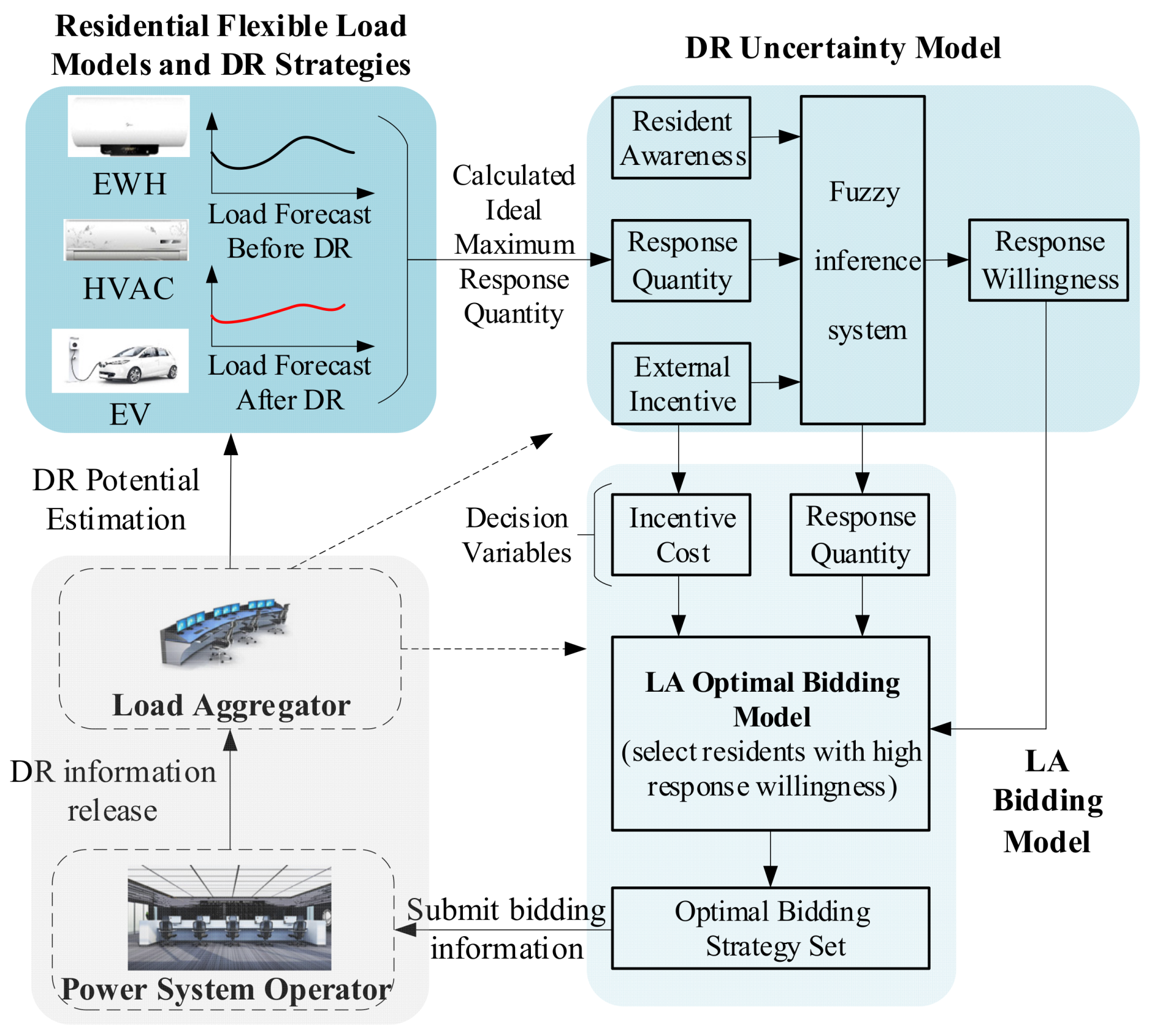
This paper focuses on how the LA formulates the optimal bidding strategy considering the uncertainty of residents’ participation in DR. The framework includes three parts: residential flexible load models and DR strategies, DR uncertainty model, and LA optimal bidding model. As shown in Figure 1, when the next-day DR information released by PSO is received, the LA needs to evaluate the response potential of the residents firstly. The LA can simulate the load curve of each resident in the DR period according to the electricity consumption information fed back by the residents and obtain the load curve after DR. The baseline load before DR can be predicted by residents’ historical load. The response potential of residents can be calculated by comparing the load curves before and after DR, which is the ideal maximum response potential. In this scenario, the aggregator ignores the willingness of residents to participate in the DR and assumes that all residents participate in the next day’s DR. In fact, the responses of residents are quite random. If the willingness of residents to respond is not considered, there is a great risk that the LA’s next day response will not meet the standard, which greatly reduces the LA’s income. Therefore, on the basis of the ideal maximum response potential, this paper considers the residents’ awareness level and the external incentive received by residents. The evaluation model of residents’ response willingness is constructed by using a fuzzy inference system. Then, combined with residents’ willingness to respond, this paper proposes an optimal bidding model, which can consider the response willingness of residents and make more residents respond with the lowest incentive cost. In the end, the LA can get more profits. The three parts are described in detail in Section 3, Section 4 and Section 5.
3. Residential Flexible Load Models and DR Strategies
3.1. HVAC Load
A thermodynamic model of the building to which the HVAC belongs is constructed using equivalent thermal parameters based on circuit simulation [17]. The differential equation form of the equivalent thermodynamic model of the HVAC can be derived in Equation (1).
where is the indoor temperature at time t, °C; is the outdoor temperature at time t, °C; is the indoor equivalent thermal resistance, °C/W; is the indoor equivalent heat capacity, J/°C; is the cooling or heating energy of the HVAC at time t, W.
Assume that the outdoor temperature is and remains constant during the time period . The indoor temperature at time can be obtained by solving Equation (1) with as the initial value.
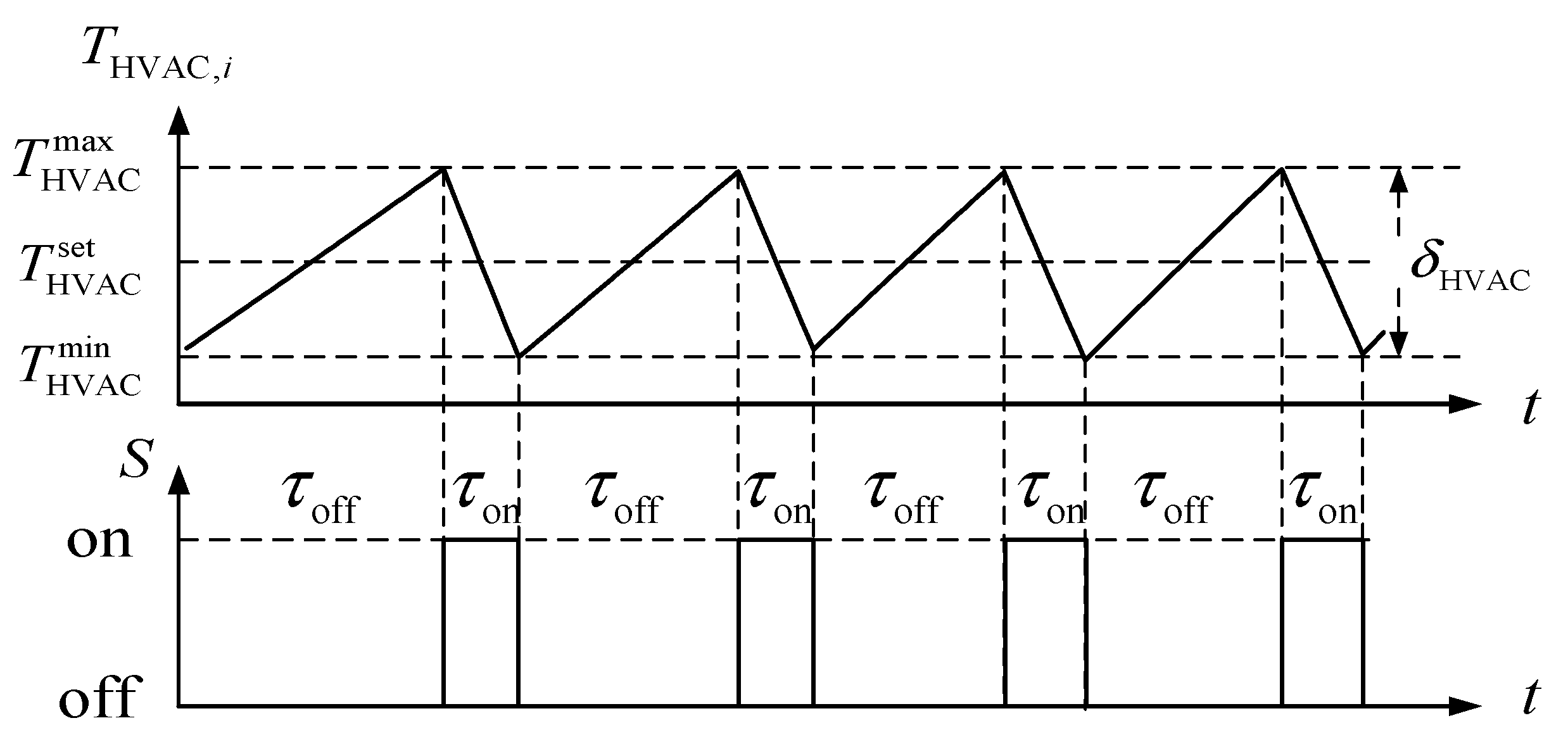
The user determines the indoor setting temperature according to comfort level, and the relationship between the operating state of the HVAC and indoor temperature is shown in Figure 2. The upper and lower limits of temperature are and , is the parameter that characterizes the control precision of a constant temperature controller.
Since the short-term change of the temperature in the house will not make the human body have a greater perception, taking refrigeration as an example, the DR strategy of the HVAC is mainly to increase the setting temperature within the period of DR to achieve the purpose of decrease load. Figure 3 shows the operating state and indoor temperature changes of the HVAC after changing the setting temperature. It can be found that the total operating time of the HVAC decreases significantly after increasing the setting temperature.
The demand response project is carried out in a period of time. In the case of refrigeration, the user changes the setting temperature at the beginning of the demand response. At the end of the demand response, the user restores the original setting temperature. The reduced electricity consumption of the HVAC of the user i during the period j is obtained by Equation (2), which is used as the calculation index of the LA’s incentive compensation to users.
where is the electricity consumption of the HVAC of the user i before DR, kWh. can be predicted by the user’s historical loads. is electricity consumption of the HVAC after DR, kWh, which is the actual electricity consumption of the user during the period j. is the difference of electricity consumption of the HVAC before and after DR in period j, kWh.
In addition, a large number of HVAC loads change the setting temperature at the beginning of the demand response, which will lead to sharp load changes. At the end of the demand response period to restore the original setting temperature, there will be load rebound phenomenon. Therefore, in this paper, the LA adopts the method of rotation control to determine the demand response period and the change of temperature setting value for each HVAC user, so as to avoid the phenomenon of sudden increase and decrease of load [18].
3.2. EWH Load
The temperature of hot water in the EWH changes reciprocally within a certain temperature range up and down the setting temperature point. Based on the equivalent thermal parameter model, the differential equation of the EWH can be constructed [19], as shown in Equation (3).
where A is the surface area of water storage tank, m2; is water density, kg/m3; cp is specific heat capacity of water, J/(kg °C); R is equivalent thermal resistance of water storage tank, °C/W; C is equivalent heat capacity, J/°C; R and C can be calculated by the 24-h inherent energy consumption coefficient ε24 and volume V of the EWH; is the heating power, W; is water temperature in the EWH, °C; is temperature outside the EWH, °C; is cold water temperature, °C; WO is water consumption of user, m3/s.
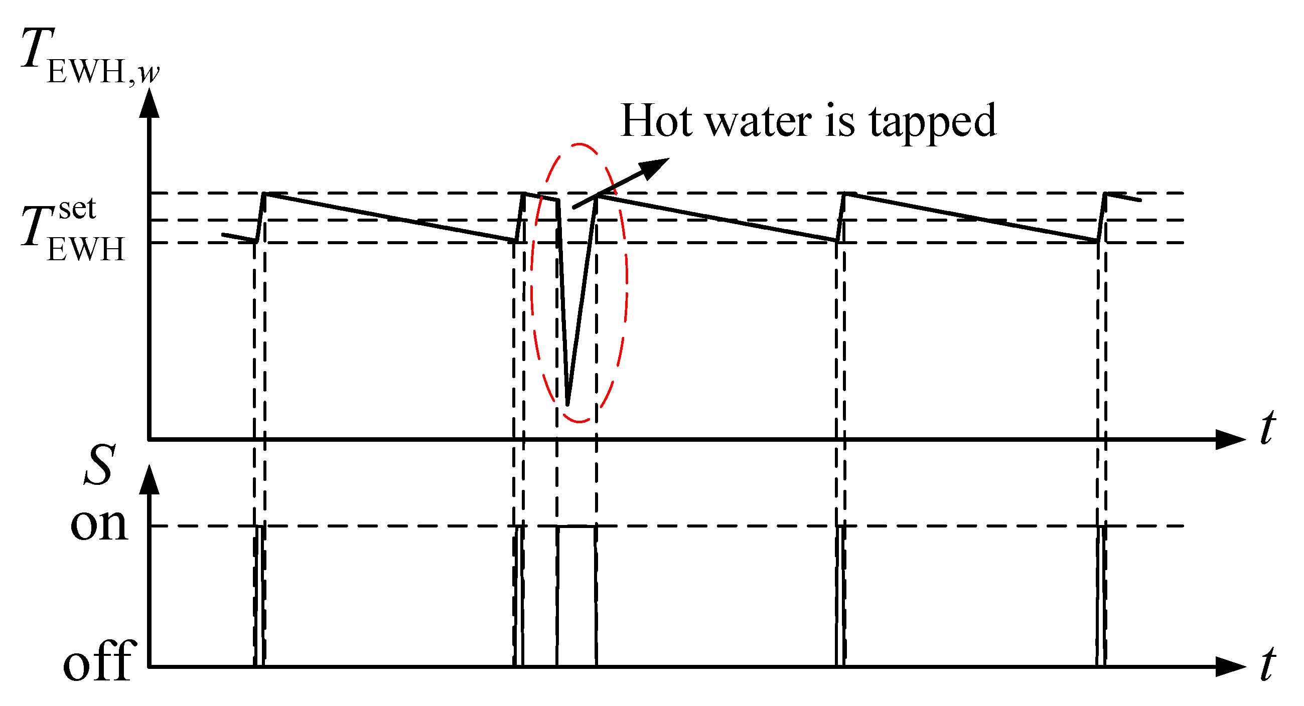
When the EWH is running, the thermostat controller is used to keep the water temperature constant, and the user determines the setting temperature . During a certain period of time, the working state of the EWH can be divided into two types depending on whether the hot water is tapped. The EWH remains heated while the hot water is tapped. Otherwise, the EWH only needs to keep the water temperature constant. Figure 4 shows the relationship between the running state of the EWH and the water temperature in the storage tank.
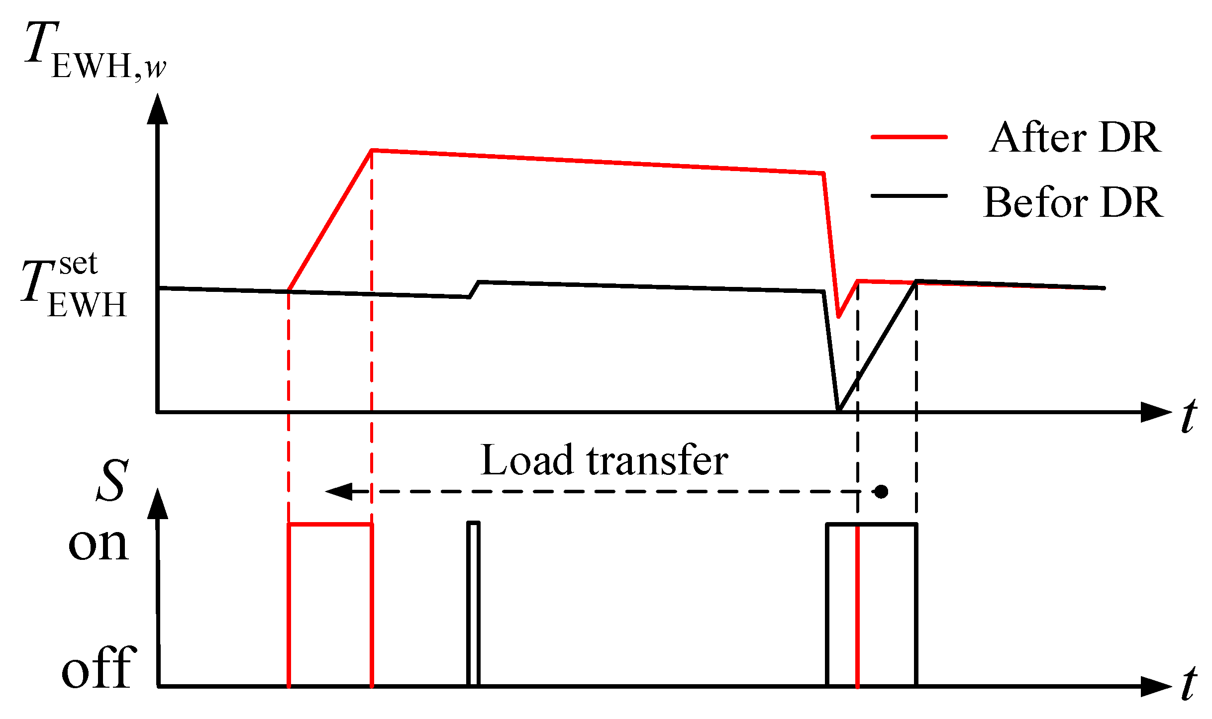
The EWH has good thermal energy storage characteristics and can participate in DR by changing the setting temperature value and heating in advance. After analysis, it is found that changing the setting temperature value has little effect on the power operation of the EWH, while heating in advance can well achieve the effect of load transfer. Therefore, the EWH participates in DR by heating in advance, as shown in Figure 5. Before and after DR, the EWH electricity consumption change value of user i is in period j.
Establishing higher temperatures will increase thermal losses and reduce the efficiency of the EWH. This section takes an EWH as the research object and analyzes the effect of increasing the setting temperature value on the efficiency. The volume V of the EWH is set to 80 L, is set to 2 kW, and are set to 20 °C and 15 °C, ε24 is set to 0.8. The setting temperature value is initially set at 55 °C, and it is raised to 70 °C from 1:00 a.m. to 5:00 a.m., which can achieve the effect of load transfer. Before and after DR, the operation state of the EWH and water temperature change curve are shown in Figure 6.
In two scenarios, the electricity consumption of the EWH can be calculated, as shown in Table 1. Due to the increase of thermal losses, the electricity consumption also responds to the increase. After DR, the electricity consumption in all day of the EWH is 6.80 kWh, which is 2.6% more than before DR. However, during the low electricity consumption period from 1:00 a.m. to 5:00 a.m., the load increased by 1.67 kwh, which is 25.2% of electricity consumption in all day. For residents, although the electricity consumption increases, the compensation for residents participating in DR is far greater than the increase of electricity cost. The increase of thermal losses has little influence on the overall income of residents, so it can be ignored.
3.3. EV Load
The model of EV is the relationship between the state of charge (SOC) of the vehicle power battery and the charging power [20]. According to the charging process of the EV, the initial constant power charging time accounts for most of the total time, so it is assumed that the EV is charged with constant power. If the EV is charged with a constant power at time t, the SOC at time t can be obtained by Equation (4).
where , , are charging power, charging efficiency and battery capacity of the EV i.
For residential consumers, the remaining power of the EV at home is mainly determined by the daily mileage. Assuming that the battery power of the EV decreases at a constant rate during the driving process, the relationship between the current SOC of the EV and the mileage of the EV after the last charge is Equation (5).
where is the initial SOC of the EV i in period j + 1; is SOC of the EV i after charging in period j; d is the driven distance of the EV i; D is endurance mileage of EV i.
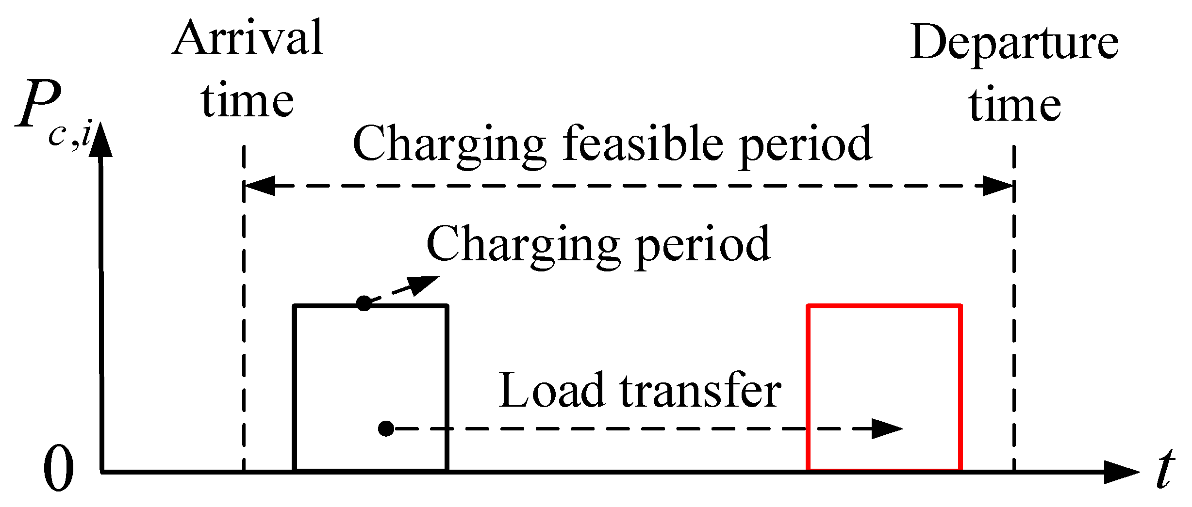
The EV can participate in DR by transferring charging time. While meeting user travel needs, the charging time can be flexibly adjusted according to the operating characteristics of the grid, as shown in Figure 7. Before and after DR, the EV electricity consumption change value of user i is in period j.
4. DR Uncertainty Model
DR potential refers to the ability of consumers to participate in response to load adjustment, including load increase and load reduction. Due to the randomness of residential consumers’ electricity consumption, there are many uncertainties in their willingness to participate in DR projects. The LA accurately estimates the response potential and response willingness of consumers and can better formulate day-ahead bidding strategies. The three main factors influencing the willingness of residents to participate in DR are the response quantity, awareness and external incentive [21,22]. The response quantity factor refers to the responsiveness of residents during the DR period, which can be calculated by , , . When the response quantity of residents is low, the willingness of residents to participate in DR is low, otherwise it is high. Awareness factors include two aspects. One is the degree of subjective identification of the residents themselves to DR, and the other is the consideration of the residents’ herd mentality, that is, the degree of identification of the surrounding environment to DR. Both can be obtained by means of questionnaire surveys. When residents’ awareness level is high, residents’ willingness to participate in DR is high. The external incentive factor is the compensation that residents get after participating in DR. In this paper, the compensation that residents get is paid by the LA.
It can be found that there are many influencing factors affecting residents’ willingness, and the randomness of residents’ willingness is large. Reference [23] adopted questionnaire survey and data statistics to analyze the DR willingness of typical urban residents, which is difficult to implement and the data set is not wide enough. In addition, there are expert judgment method, analytic hierarchy process (AHP), fuzzy comprehensive evaluation method (FCEM), dynamic weighted round-robin (DWRR) and other non-data-driven methods. These methods can consider a variety of factors and build an evaluation model of residents’ willingness to participate in DR. However, there are some problems in the above methods, such as the influence of subjective experience, one-sided results, low precision, low efficiency and lack of real-time performance. With the development of artificial intelligence, data-driven and machine learning methods represented by artificial neural network (ANN), extreme learning machine (ELM) and support vector machine (SVM) have been widely applied in many aspects [24]. However, these models need high requirements for data quantity and representativeness, and the mobility of the models between different residential communities is relatively poor. In the early stage of demand response, it is difficult to obtain a large amount of data such as residents’ electricity consumption behavior and willingness. Fuzzy inference system can consider the advantages of both non-data-driven and data-driven methods. In the initial stage of DR, the fuzzy inference system is mainly built by expert experience in the absence of sample data. Then, an adaptive neuro-fuzzy inference system (ANFIS) can be constructed based on the user’s electricity consumption data and willingness data combined with the neural network. Neural network is used to adjust the parameters of fuzzy inference system to make the evaluation result of willingness more accurate, [25].
This paper uses a fuzzy inference system to establish the relationship between residents’ willingness to participate in DR and influencing factors, so as to construct DR uncertainty modeling. The fuzzy inference system imitates human thinking mode and is easy to understand and use. As a universal approximation system, fuzzy inference system can approximate any non-linear system with arbitrary precision in a closed bounded domain. Therefore, it can obtain satisfactory results under the condition of insufficient input. Enhancement of fuzzy inference systems is ANFIS, which can either purpose a validation of the fuzzy inference system or train it by modifying the parameters according to a chosen error criterion.
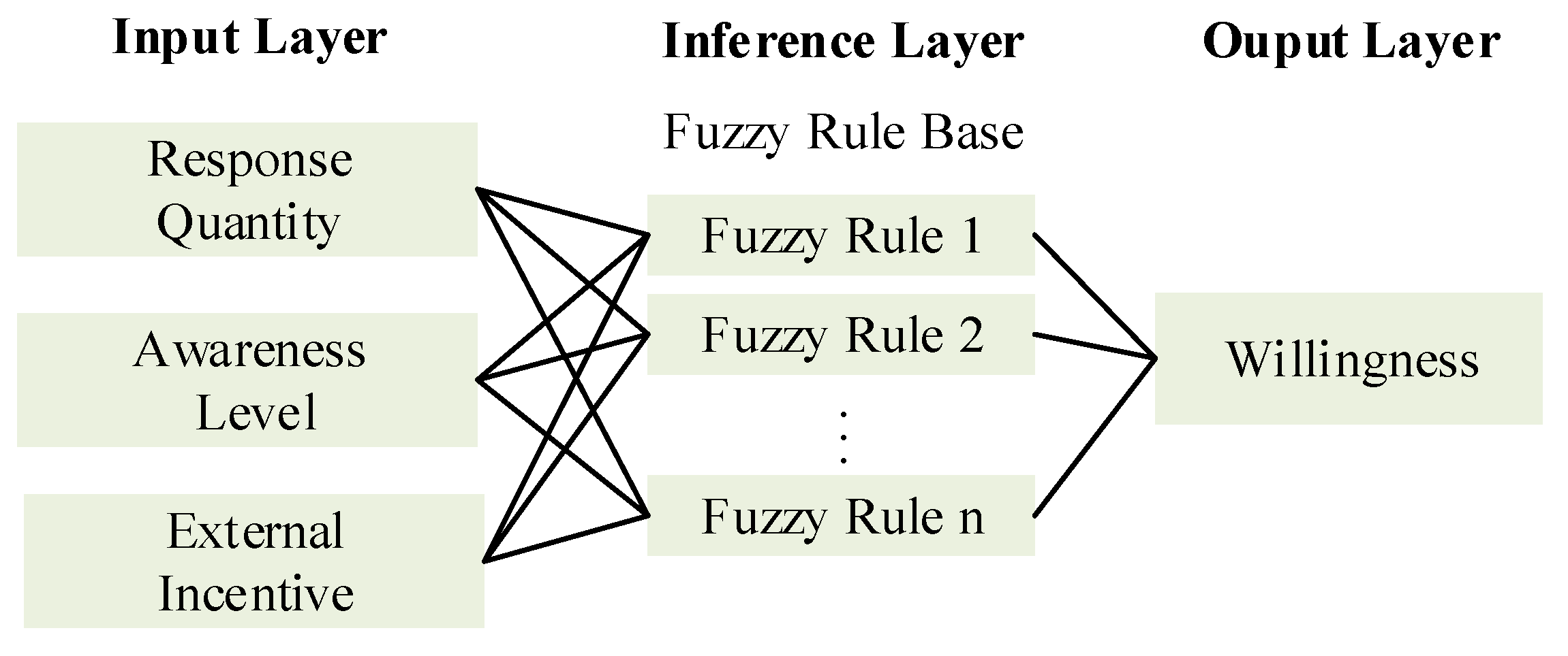
The fuzzy inference system can be divided into three layers: the input layer, the fuzzy inference layer and the output layer, as shown in Figure 8. In the input layer, the input values are transformed into membership degrees of each set through membership function, and this process is fuzzy. The fuzzy inference layer uses an if–then framework to establish a fuzzy reasoning rule library base for fuzzy reasoning. In this paper, Mamdani type fuzzy inference is used. The output layer is the weighted average or sum of all rule outputs, depending on the respective defuzzification method applied [26].
The input variables are normalized to the range of [0,1] by Equation (6) and transformed into the same order of magnitude and dimension, which is convenient for the subsequent calculation of the model.
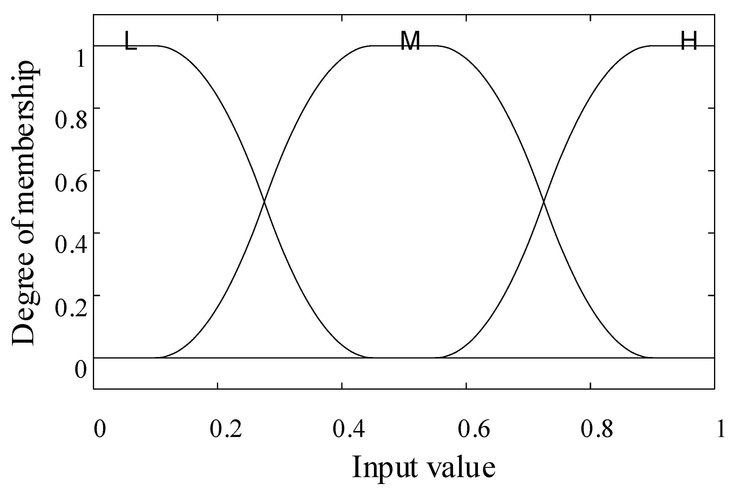
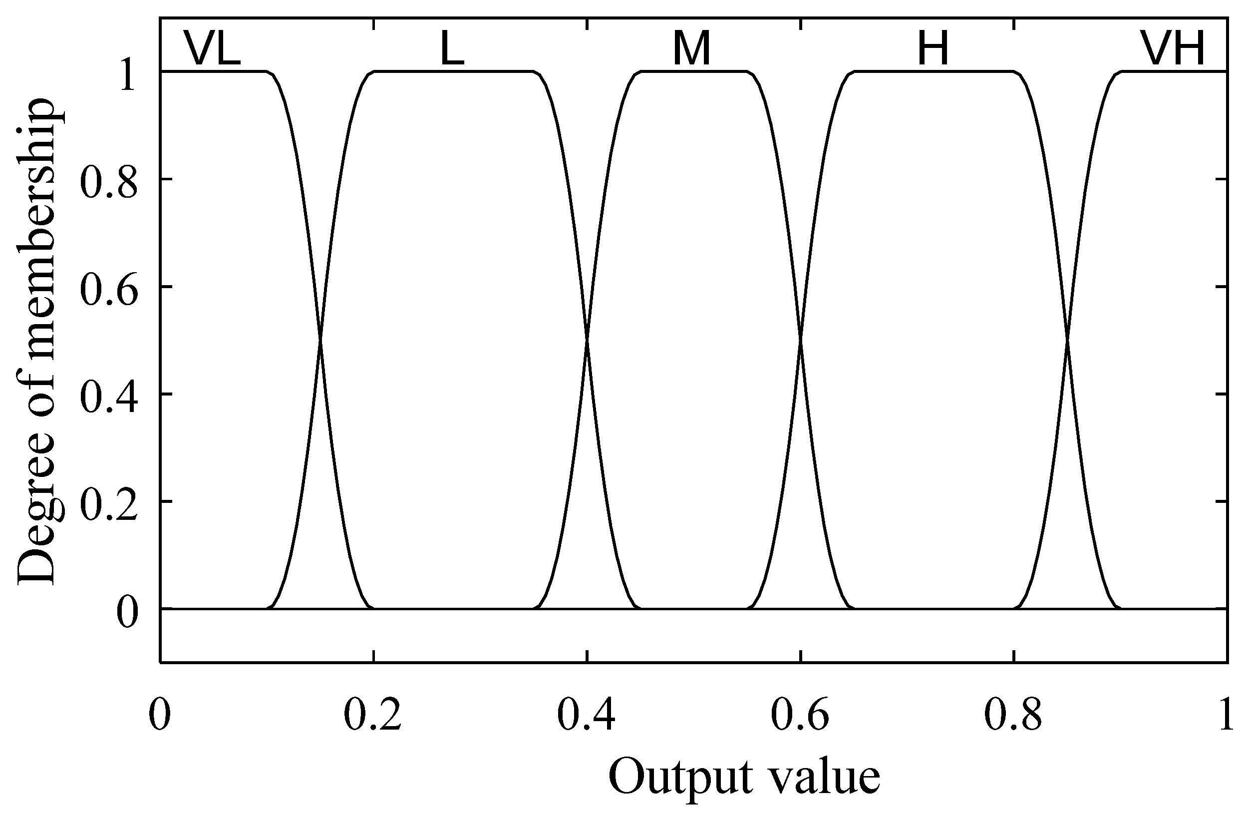
The input influencing factor values are divided into three levels of high, medium and low by the membership function [27], as shown in Figure 9. Instead of using the familiar sharp-edged Boolean logic, the input values can also be converted to an intermediate value between the two levels just as humans make decisions. Different input data correspond to different membership degrees of the fuzzy level. For example, when the input data is 0.3, it belongs to level L to a degree of 0.5 and to level M to a degree of 0.5. When the input data is greater than 0.9, it will be fully subordinate to level H. In this way, all input variables are blurred. Because the precision of the output variable is relatively high, the output participation value is divided into five levels, as shown in Figure 10. The level VH indicates the highest willingness of residents to respond, and the level VL indicates the lowest willingness of residents to respond.
Input and output are connected through the fuzzy inference rule base in Table 2. In form of linguistic if–then statements without employing precise quantitative analyses, the fuzzy inference rules imitate human thinking. An example that describes such a rule is “If Response Quantity is L, Awareness Level is L, and External Incentive is also L, then the Willingness is VL”. Other rules follow this line of reasoning.
5. LA Bidding Model
The power company releases DR bidding information for the next day, including load increase or load decrease. The LA simulates the response mode of residential consumers and estimates response potential and response willingness of residents. On this basis, the LA formulates the optimal bidding strategies with the largest net profit and participate in this bidding [28,29]. This section will build the LA bidding model and propose a method to formulate the optimal bidding strategy.
5.1. Objective Function
The net profit of the LA can be calculated by the income value, the incentive expenditure value, and the compensation value, which can be obtained by Equations (7)–(12).
where is the net profit obtained by the LA k. , , are the income value obtained by the LA k, the incentive expenditure value of the compensation consumer, and the compensation value caused by the response exceeding the limit in period j; , , are bidding capacity, bidding unit price, and incentive unit price of the LA k in period j; is the willingness of resident i to participate in DR during the period j; is average participation willingness of n residents in period j; is the unit price of compensation in response to the out-of-limit part.
The income value is paid by the PSO to the LA, which can be calculated by multiplying the bidding unit price and the bidding capacity. The incentive expenditure value is the LA’s compensation for residents’ participation in DR, which is the part of the LA’s cost and can be calculated by multiplying the incentive unit price and the bidding capacity. In addition, if the LA fails to reach the response volume declared in the previous bidding, the PSO will impose a fine on the LA. The total amount of the fine is the LA’s compensation value. Considering the uncertainty of the actual response of residents, the LA is allowed to have a response deviation margin in the bid winning capacity. Suppose the ratio of the lowest response amount to the winning bid capacity is , and the LA does not need to compensate within the deviation margin. The compensation value can be obtained by Equation (11).
5.2. Constraints
5.2.1. Bidding Capacity Constraint
The LA’s bidding capacity needs to be smaller than the theoretical maximum responsive potential of the residents. The constraint is shown in Equation (13).
where N is the number of all consumers managed by the LA.
5.2.2. Bidding Unit Price Constraint
Because there is more than one LA bidding in the same DR period, the LA will fail to win the bid due to the high bidding unit price. To simplify this process in the paper, the LA only determines the bidding unit price based on the response cost, without considering the influence of other LAs on the bidding unit price. The constraint is shown in Equation (14).
where , are the minimum and maximum bidding unit price of the LA in period j.
5.2.3. Incentive Unit Price Constraint
According to consumer psychology, the influence of incentive level on residents’ willingness to participate in DR can be divided into three stages: dead zone, response zone and saturation zone. When the incentive is less than the dead zone threshold, the residents’ willingness to participate in DR is zero. When the incentive is greater than the dead zone threshold and less than the saturation threshold, the residents’ willingness increases with the increase of incentive. When the incentive unit price is greater than the saturation value, the influence of incentive factor on residents’ willingness will no longer change [12,13,14,15]. In addition, excessively high incentive unit price leads to higher response costs and lower net income for the LA. Therefore, it is necessary to restrict the incentive unit price of LA, which is shown in Equation (15).
where is the saturation value of the LA’s incentive compensation for residents’ willingness to participate in DR.
5.3. The Process of Optimal Bidding Decision-Making
Based on the LA bidding model, the LA selects residential groups, determines the incentive cost, the bidding quantity, and formulates the optimal bidding strategy. The specific process is as follows:
- Divide residents into different groups according to their different awareness level.
- Use the fuzzy inference system to evaluate the participation willingness of each group of residents, and rank the residents from high to low according to their participation willingness.
- Select the residents with high willingness to participate, and calculate the minimum incentive level that meets the constraint of response reliability.
- Add new residents with low willingness to participate, increase the response resident size, and recalculate the minimum incentive level that meets the constraint of response reliability.
- Obtain the lowest incentive levels under different response groups to form a set of bidding strategies.
- In the strategy set, choose the strategy with the highest net income and participate in the final bidding.
6. Case Study
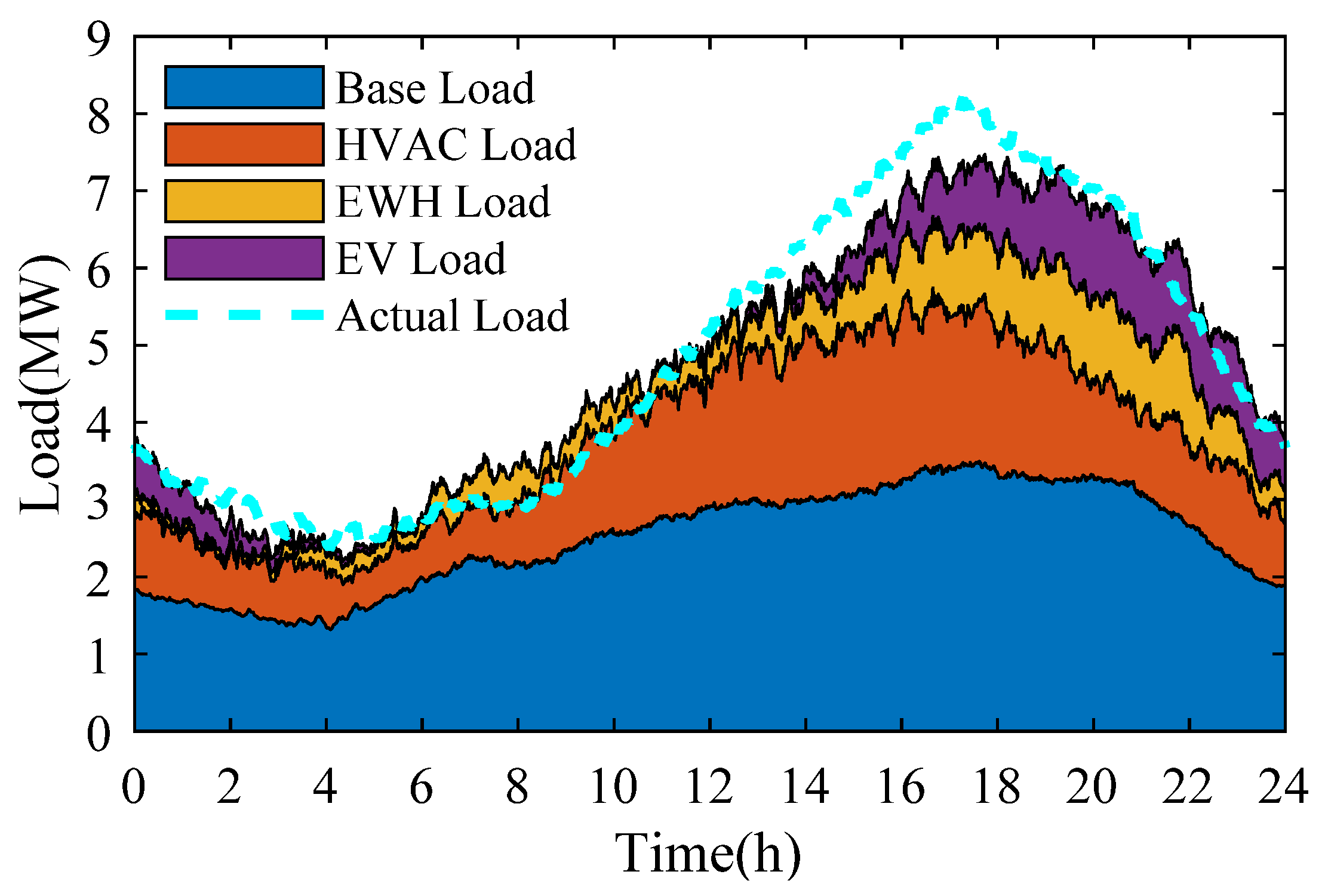
A case study is presented in this section, where the LA integrates the load resources of the residential community in a certain area and participates in demand side bidding. This community has 3000 households and contains base loads and a large number of flexible loads, mainly HVAC, EWH and EV. Compared with other seasons of the year, the total load curve of this community is at the peak in summer due to the large amount of air conditionings used by residents for cooling. Therefore, this paper selects the residential loads of the community in August in summer as the research object and simulates the DR project. Based on the actual total load curve of residents in the community, the load data of HVAC, EWH and EV are excluded, and the remaining loads are called the base loads. In this case, the actual base loads of residential community are selected as the base loads, and the loads of HVAC, EWH and EV are simulated by using the model in Section 3. The total load curve of the community is obtained by adding the base load curve and the flexible load curve. In addition, fixed tariff is used in the residential community. Based on the DR strategies of flexible loads in Section 3, the LA implements incentive DR project to residents.
6.1. Case Data Setting
To diversify EV types, with reference to EV models on the market, the battery capacity is randomly selected from 57, 19, 60, 85, 18.7, and 28 kWh. The charging power is set to 3.5 kW and the charging efficiency is set to 0.9. The daily mileage D of residents’ EVs is approximately subject to lognormal distribution: , where is 3.2; is 0.88. The arrival time of residents’ EVs is approximately subject to the normal distribution: , where is 18.8; is 3.5 [20].
The model parameters of HVAC load and EWH load are shown in Table 3, which reflect the diversity of resident load. Residents’ water use time is set in the form of probability based on statistical data, and water duration can be divided into two types, which are subject to normal distribution N (5,1) and N (1,0.1) [19].
The total load forecast curve of the residential community obtained by simulation is shown in Figure 11. By comparing the actual total load curve, it can be found that the total load curve obtained by simulation can restore the total load curve well. This indicates that the model and parameter selection of flexible equipment are reasonable and can be used as the research object of demand response simulation.
The residential load shows the characteristics of the evening peak, and the electricity consumption is low in the early morning. In order to meet the dispatching demand, the electric power company sets the period of increasing load demand: 1:00–6:00, j = 1, and setting the period of reducing load demand: 16:00–20:00, j = 2.
6.2. Results and Analysis of DR Potential and Willingness
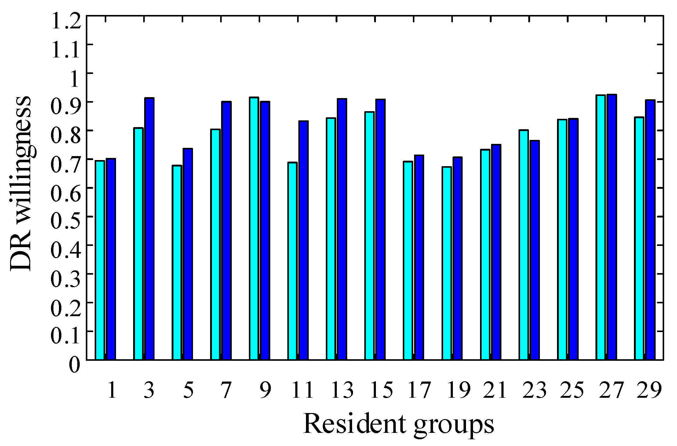
According to the latest questionnaire survey feedback, the LA obtains the residents’ DR awareness level. Due to the large resident base, if the LA uses each resident as a control variable, it will cause the disaster of the variable dimension, so the LA divides residents into different groups according to the awareness level, each group contains 100 households. The LA simulates the response plan of each resident according to the flexible load DR strategies proposed in Section 3 and obtains the response quantity of each resident group during two periods of load increase and load decrease. The response quantity and awareness level of some residential groups are shown in Figure 12. It can be found that different residents have different response quantity and awareness during the period of DR. The overall response quantity during the load increase period is greater than that during the load decrease period, because the LA considers the residents’ electricity comfort when estimating their response potential, which is not detailed in this paper due to space limitations. Therefore, during the peak period of electricity consumption, reducing a large amount of load has a greater impact on the electricity consumption of residents. While in the low period of electricity consumption, the load such as EWH and EV can be transferred to this period while meeting the needs of residents.
Based on the DR willingness evaluation model in Section 4 and Equation (12), set the incentive unit price of the LA in period 1 and period 2 to 0.8 yuan/kWh and 1.3 yuan/kWh, and the average willingness evaluation results of some residential groups in the two periods are as shown in Figure 13. Combining with Figure 12, it can be found that when there is little difference in the response quantity of the residential groups, the awareness factor largely affects the willingness to participate in DR. For example, the awareness of the 19th and 21th resident is low, and the corresponding DR willingness is also low.
6.3. Results and Analysis of LA Bidding Strategies
Referring to the actual DR project of the residential community, the ratio of the lowest response amount to the winning bid capacity is set to 0.9. The unit price of compensation in response to the out-of-limit part is set to 2 yuan/kWh. The LA does not need to be fined if the actual respond capacity is more than 90% of the bidding capacity declared in the previous bidding. Otherwise, the amount of under-response is penalized at 2 yuan/kWh. The incentive expenditure value of the compensation consumer and the compensation value caused by the response exceeding the limit together constitute the LA’s cost of financial expenditure. In this section, the results obtained by considering the resident’s response willingness are compared and discussed with the conventional results without considering the willingness. The details are as follows.
6.3.1. Bidding Strategies during the Load Increase Period
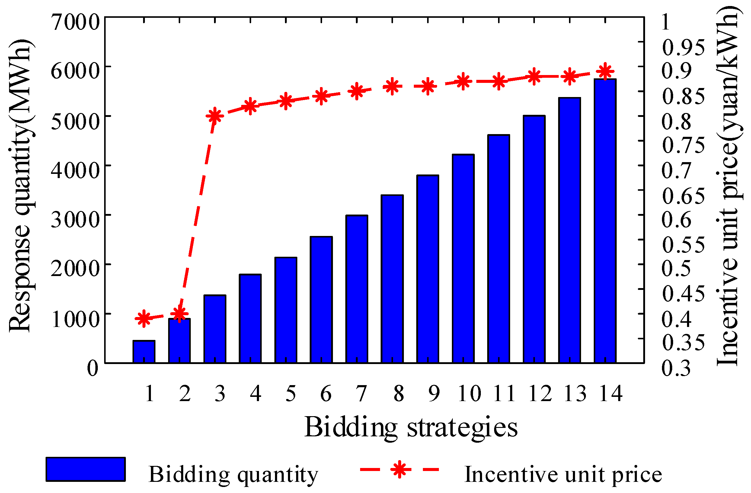
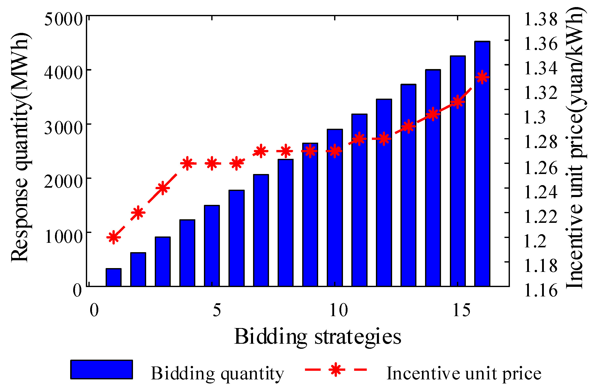
Based on the optimal bidding strategy in Section 5, the LA selects groups with high willingness to participate, and calculates the optimal bidding plan that meets the constraints of willingness to participate in residential groups of different sizes. Figure 14 shows the different bidding quantities and incentive unit prices during the load increase period, and the number of bidding strategies is 14. In each of these strategies, the average willingness of residents to participate in DR is 0.9. Therefore, the compensation value caused by the response exceeding the limit is zero. The total response cost of the aggregator is just the incentive expenditure value of the compensation consumer. It can be found that choosing the residential groups with a high level of response quantity and awareness requires the lowest incentive cost, but the total bidding quantity is low. As the number of responding residential groups is expanded, the total bidding quantity can be increased, and the required incentive cost will increase accordingly. The reason is that the response quantity and awareness level of the newly added groups are low, and higher incentives are needed, so that the willingness to participate in DR can meet the minimum constraint requirements.
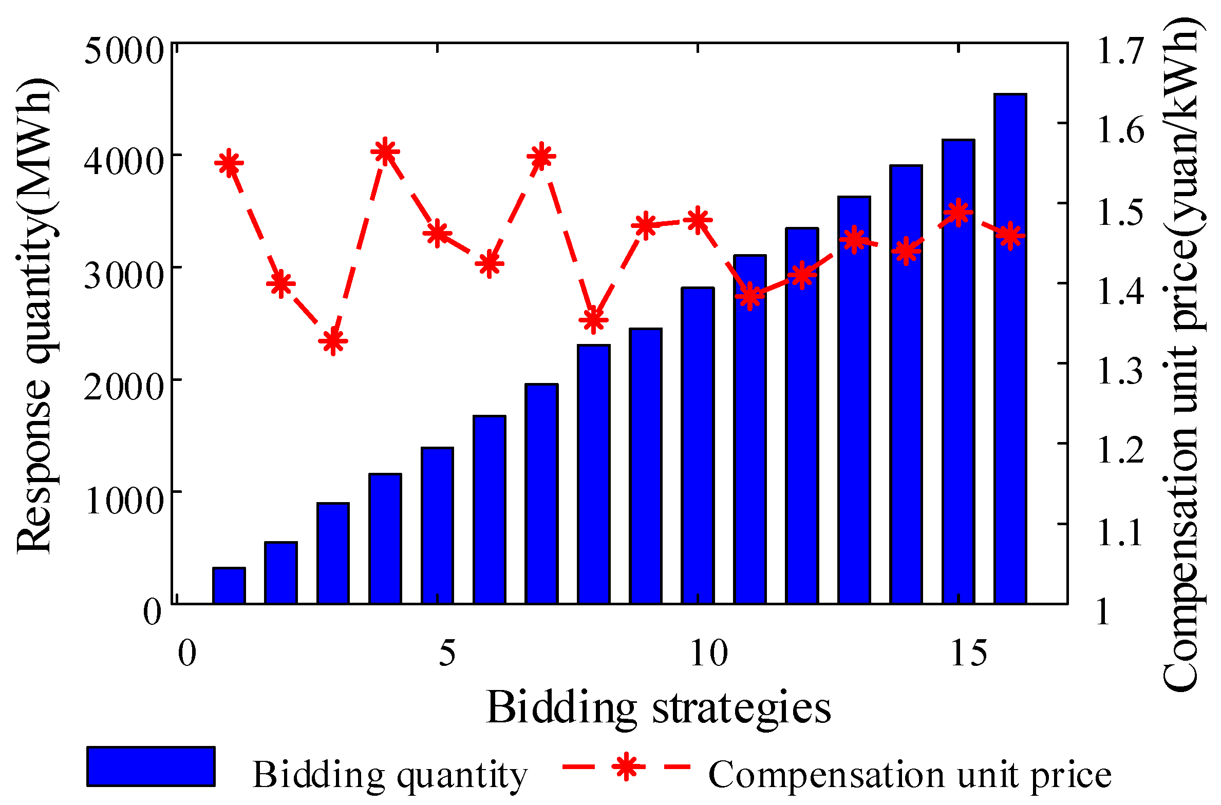
Without considering the willingness, the LA randomly selects a certain number of residents for each bidding strategy in Figure 14, so that the response capacity of the two is approximately equal. Different bidding quantity and compensation unit price are shown in Figure 15. It can be found that as the total bidding quantity is increased, the compensation unit price does not increase in response, but changes randomly. In addition, the compensation unit price without considering the willingness is greater than that considering the willingness. Table 4 shows the percentage decrease of unit price in increasing load period with considering the willingness and without considering the willingness. The response cost of LA during the load increase period is decreased by up to 71% and by an average of 40%. This is mainly because the average willingness of randomly selected residents to respond may be less than 0.9, so the response of aggregators cannot meet the standard. The compensation value caused by the substandard response adds to the LA’s total response cost.
6.3.2. Bidding Strategies during the Load Decrease Period
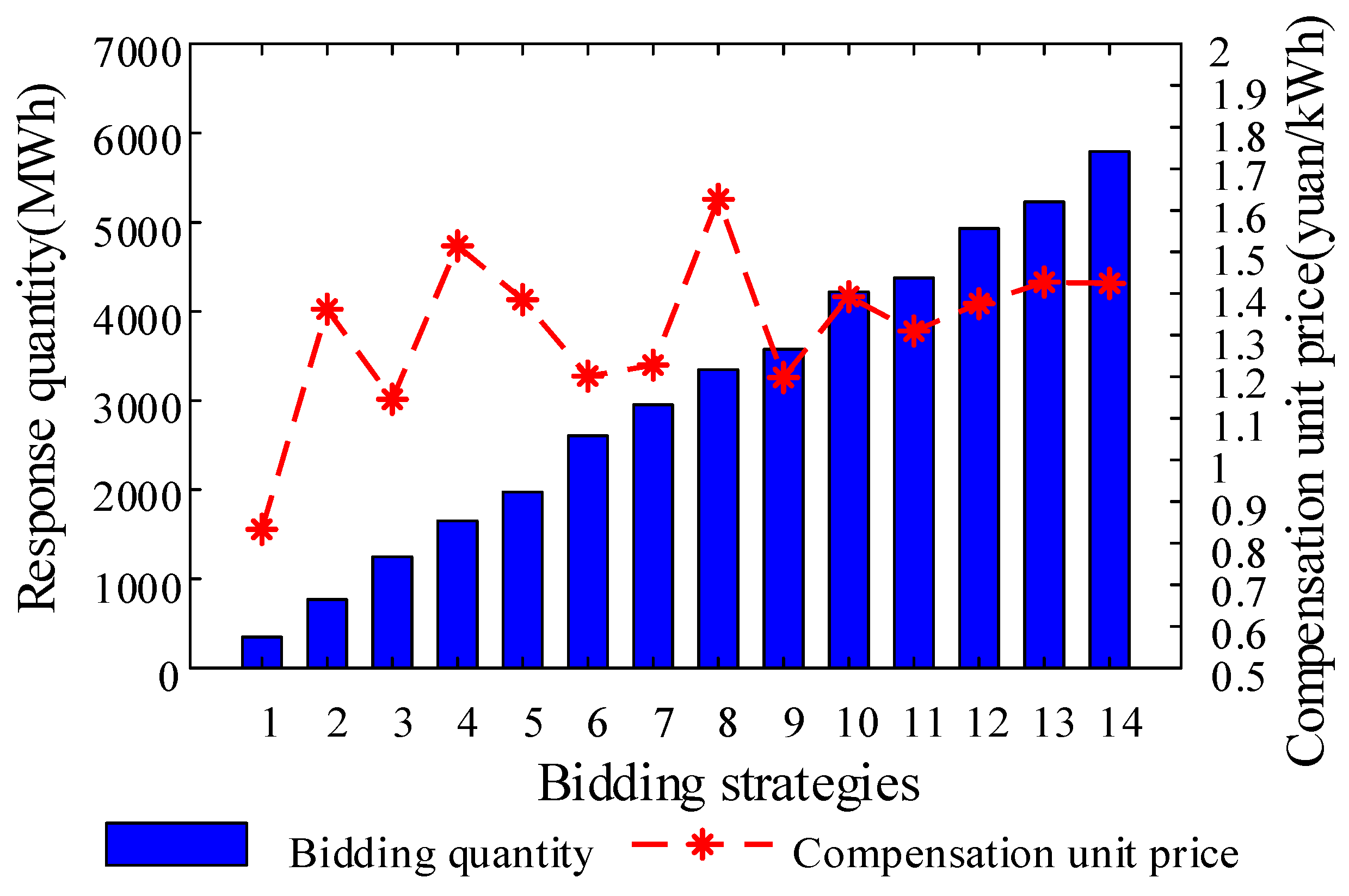
Figure 16 shows the different bidding quantities and incentive unit prices during the load decrease period, and the number of bidding strategies is 16. In each of these strategies, the average willingness of residents to participate in DR is also 0.9. As the total bidding quantity is increased, the required incentive cost is increased accordingly. Without considering the willingness, the LA randomly selects a certain number of residents for each bidding strategy in Figure 16, and different bidding quantity and compensation unit price during the load decrease period are shown in Figure 17. The compensation unit price without considering the willingness is also greater than that considering the willingness. Table 5 shows the percentage decrease of unit price in decreasing load period considering the willingness and without considering the willingness. The response cost of LA during the load decrease period is decreased by up to 23% and by an average of 12%.
6.3.3. Optimal Bidding Strategy
The LA selects the strategy with the largest net income among all the bidding strategies as the optimal decision of bidding. The optimal bidding information of the two periods is shown in Table 6. During the period from 1:00 to 6:00, the optimal quantity of load increase of residents is 5.75 MW, and the net income of the LA is 2557.48 yuan. At this time, the average willingness of residents to respond is 0.9, which is within the range of response deviation margin. During the period from 16:00 to 20:00, the optimal quantity of load decrease of residents is 4.52 MW, and the net income of the LA is 3006.91 yuan. At this time, the average willingness of residents to respond is 0.9, which is also within the range of response deviation margin.
Two scenarios are analyzed. One is considering residents’ response willingness and simulating that some residents will participate in the next day’s DR according to Table 6. The other is simulating that all residents will participate in DR without considering residents’ response willingness; the conventional bidding strategies are shown in Table 7. During the period from 1:00 to 6:00, the conventional quantity of load increase of residents is 12.26 MW, and the net income of the LA is −59.25 yuan. At this time, the average willingness of residents to respond is 0.81, which is not within the range of response deviation margin. As a result, the LA is fined, which results in a negative net profit for the LA. During the period from 16:00 to 20:00, the net profit of conventional bidding strategy is far less than the net profit of optimal bidding strategy.
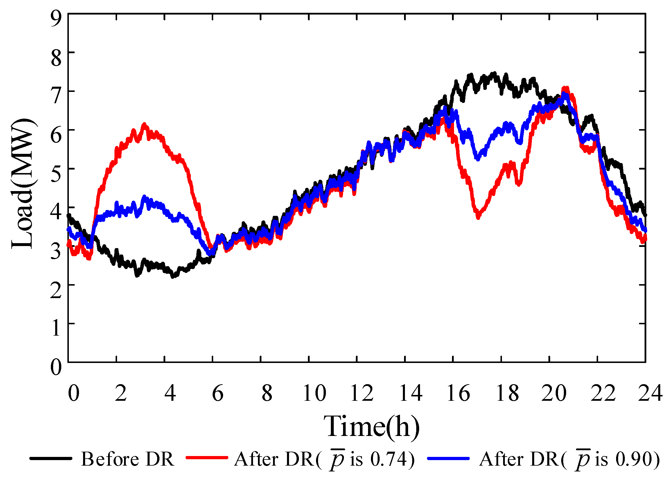
The changes of the power curve after residents participate in DR under two scenarios are shown in Figure 18. Assuming that all residents participate in DR, the load curve changes the most, but the average response willingness of the residents is 0.74, which is not within the response deviation margin. Therefore, the risk of under-response or over-response in the next day is greater. On the one hand, this will reduce the revenue of the LA; on the other hand, it is not conducive to the power company to ensure the balance of power supply and load demand. Therefore, the LA estimates the residents’ willingness to respond, and then selects the residents with high willingness to response, which can reduce the risk of compensation the next day and achieve the greatest benefit.
6.3.4. Summary of the Impact of Resident Response Uncertainty
In the demand side bidding, without considering the willingness of residents to respond, the LA bids for respond quantity based on the ideal maximum response potential of residents, which may make the actual response quantity of the LA the next day less than the previous bidding quantity. This is because the willingness of residents to participate in DR is different, and it is costly for the LA to involve all residents in DR. Therefore, the LA need to consider the residents’ willingness and choose the residents with high response willingness to participate in DR, which can greatly reduce the demand response cost of the LA. The case simulation in this section shows that without considering the uncertainty of residents’ participation in DR, the LA’s eventual net income would be substantially reduced, perhaps even negative. However, considering the uncertainty of the residents’ response, the LA prefers to choose the residents with high willingness to participate in the response, which can reduce the response cost of the LA and increase net income. The response cost of LA during the load increase period is decreased by up to 71% and by an average of 40%; and during the load decrease period is decreased by up to 23% and by an average of 12%.
In addition, to quantify the uncertainty of the residential consumers, the uncertainty evaluation model considers the three influences of residents’ consciousness, response capacity and external incentive. Compared with the model based on consumer psychology, which only considers external incentives, the model presented in this paper is more representative of the actual situation. It is found that there is little difference in the response quantity of different residential groups. Therefore, the awareness factor is the main reason for the difference in response willingness. From the LA’s perspective, at the beginning of the DR, the LA can increase residents’ willingness to participate in DR projects by increasing engagement of familiar residents, increasing publicity and promotion of favorable news about DR, supporting relevant policies, and increasing financial subsidies to residents. Then, the LA can obtain data on residents’ electricity usage behavior and DR participation in a large number of historical DR projects. Combined with the artificial neural network, the LA can adjust the parameters of the fuzzy inference system, which can more accurately assess the residents’ response uncertainty.
7. Conclusions
In this paper, considering the uncertainty of residential consumers’ participation in DR, an optimal bidding decision-making model is constructed to maximize the LA’s income in demand side bidding. Specifically, the physical models of flexible loads are established to evaluate the ideal DR potential firstly. It is found that the overall response quantity of residential consumers during the load increase period is greater than that during the load reduction period. Then, on the basis of the ideal DR potential, this paper also considers the residents’ awareness level and the external incentive to construct a fuzzy inference model for the LA to evaluate residents’ response willingness. Finally, combined with residents’ willingness to respond, this paper proposes an optimal bidding model for the LA. Simulation results indicate that considering the impact of the residents’ DR uncertainty, the final bidding response quantity selected by the LA will be reduced to a certain extent compared with not considering DR uncertainty, but the average willingness of the residents will be improved, which can reduce the risk of under-response or over-response the next day and reduce the DR cost. The response cost of LA during the load increase period is decreased by up to 71% and by an average of 40%; and during the load decrease period, it is decreased by up to 23% and by an average of 12%. Subsequent research work can further consider the competitive game among various LAs based on this article, and guide for the LAs’ participation in demand side bidding.
Author Contributions
Conceptualization, Z.S. and J.S.; methodology, Z.S.; software, Z.S.; validation, S.L.; formal analysis, Z.C.; investigation, W.Y.; resources, Z.Z.; data curation, Z.S.; writing—original draft preparation, Z.S.; writing—review and editing, Z.S.; visualization, Z.S.; supervision, J.S.; All authors have read and agreed to the published version of the manuscript.
Funding
This research received no external funding.
Conflicts of Interest
The authors declare no conflict of interest.
References
- Kang, C.; Yao, L. Key scientific issues and theoretical research framework of high-proportion renewable energy power systems. Autom. Electr. Power Syst. 2017, 41, 2–11. [Google Scholar]
- Wang, K.; Yao, J.; Yao, L.; Yang, S.; Yong, T. Review of research on flexible load dispatch. Autom. Electr. Power Syst. 2014, 38, 127–135. [Google Scholar]
- D’hulst, R.; Labeeuw, W.; Beusen, B.; Claessens, S. Demand response flexibility and flexibility potential of residential smart appliances: Experiences from large pilot test in Belgium. Appl. Energy 2015, 155, 79–90. [Google Scholar] [CrossRef]
- Wang, P. Research on consumers’ response characters and ability under smart grid: A literatures survey. Proc. CSEE 2014, 34, 3654–3663. [Google Scholar]
- Ellabban, O.; Abu-Rub, H. Smart grid customers’ acceptance and engagement: An overview. Renew. Sustain. Energy Rev. 2016, 65, 1285–1298. [Google Scholar] [CrossRef]
- Hu, Q.; Li, F.; Fang, X. A framework of residential demand aggregation with financial incentives. IEEE Trans. Smart Grid 2018, 9, 497–505. [Google Scholar] [CrossRef]
- Liu, X.; Gao, B.; Li, Y. Bayesian Game-Theoretic Bidding Optimization for Aggregators Considering the Breach of Demand Response Resource. Appl. Sci. 2019, 9, 576. [Google Scholar] [CrossRef] [Green Version]
- Chen, S.; Chen, Q.; Xu, Y. Strategic bidding and compensation mechanism for a load aggregator with direct Thermostat Control Capabilities. Trans. Smart Grid 2018, 9, 2327–2336. [Google Scholar] [CrossRef]
- He, X.; Liu, X.; Wang, Q.; Sun, W. Research on Scheduling Strategy of Load Aggregator Considering Priority Classification of Electricity Consumption Satisfaction. Power Syst. Technol. 2020, 1–9. [Google Scholar] [CrossRef]
- Wen, G.; Weng, W.; Zhao, Y.; Jiang, C. A bi-level optimal dispatching model considering source-load interaction integrated with load aggregator. Power Syst. Technol. 2017, 41, 3956–3962. [Google Scholar]
- Liu, X.; Gao, B.; Luo, J.; Tang, Y. Resident load hierarchical dispatch model based on non-cooperative game. Autom. Electr. Power Syst. 2017, 14, 54–60. [Google Scholar]
- Sun, D.; Wang, Y.; Wang, P.; Li, Y.; Xiao, Y. A multi-timescale source-charge interactive decision making method considering the uncertainty of demand response. Autom. Electr. Power Syst. 2018, 42, 106–113. [Google Scholar]
- Wang, P.; Li, Y.; Li, Y.; Dou, X. Interruptible load considering response uncertainty participates in coordinated optimization of system standby configuration. Electr. Power Autom. Equip. 2015, 35, 82–89. [Google Scholar]
- Zhu, L.; Liu, S.; Tang, L.; Ji, J.; Hang, C. Uncertain response modeling of charge and discharge and day-ahead scheduling strategy of electric vehicle agents. Power Syst. Technol. 2018, 42, 3305–3314. [Google Scholar]
- Vallés, M.; Bello, A.; Reneses, J.; Frías, P. Probabilistic characterization of electricity consumer responsiveness to economic incentives. Appl. Energy 2018, 216, 296–310. [Google Scholar] [CrossRef]
- Wu, Q.; Li, Y.; Yao, S.; Qiao, L.; Guo, W. Research on conformity influence of power consumers participating in demand response. Dema. Side Manag. 2016, 18, 14–21. [Google Scholar]
- Zhou, X.; Shi, J.; Tang, Y.; Li, Y.; Li, S.; Gong, K. Aggregate Control Strategy for Thermostatically Controlled Loads with Demand Response. Energies 2019, 12, 683. [Google Scholar] [CrossRef] [Green Version]
- Koutitas, G. Control of Flexible Smart Devices in the Smart Grid. IEEE Trans. Smart Grid 2012, 3, 1333–1343. [Google Scholar] [CrossRef]
- Sun, J.; Tang, S.; Liu, F.; Wang, D.; Wang, R. Modeling Method and Control Strategy Evaluation of Electric Water Heater for Demand Response Program. Autom. Electr. Power Syst. 2016, 28, 51–55.a. [Google Scholar]
- Zhang, J.; Yan, J.; Liu, Y.; Zhang, H.; Lv, G. Daily electric vehicle charging load profiles considering demographics of vehicle users. Appl. Energy 2020, 274, 115063. [Google Scholar] [CrossRef]
- Yang, X.; Zhou, M.; Li, G. Survey on demand response mechanism and modeling in smart grid. Power Syst. Technol. 2016, 40, 220–226. [Google Scholar]
- Parrish, B.; Heptonstall, P.; Gross, R.; Sovacool, B.K. A systematic review of motivations, enablers and barriers for consumer engagement with residential demand response. Energy Policy 2020, 138, 111221. [Google Scholar] [CrossRef]
- Miloš, R.; Zorica, B.; Marijana, D.; Aleksandra, L. Assessing consumer readiness for participation in IoT-based demand response business models. Technol. Forecast. Soc. Chang. 2020, 150, 119715. [Google Scholar] [CrossRef]
- Zhu, T.; Ai, Q.; He, X.; Li, Z.; Sun, D.; Li, X. An Overview of Data-driven Electricity Consumption Behavior Analysis Method and Application. Power Syst. Technol. 2020, 44, 3497–3507. [Google Scholar]
- Holtschneider, T.; Erlich, I. Modeling Demand Response of Consumers to Incentives Using Fuzzy Systems. In 2012 IEEE Power and Energy Society General Meeting; IEEE: New York, NY, USA, 2012; pp. 1–8. [Google Scholar] [CrossRef]
- Kaluthanthrige, R.; Rajapakse, A.D. Use of Probabilistic Fuzzy Inference Systems to Model Demand Response in the Off-Grid Power Systems of Northern Canada. In Proceedings of the 2019 14th Conference on Industrial and Information Systems (ICIIS), Kandy, Sri Lanka, 18–20 December 2019; IEEE: New York, NY, USA, 2019; pp. 419–424. [Google Scholar] [CrossRef]
- Sumaiti, A.; Konda, S.R.; Panwar, L. Aggregated Demand Response Scheduling in Competitive Market Considering Load Behavior Through Fuzzy Intelligence. IEEE Trans. Ind. Appl. 2020, 56, 4236–4247. [Google Scholar] [CrossRef]
- Bruninx, K.; Pandžić, H.; Cadre, H.; Delarue, E. On the Interaction Between Aggregators, Electricity Markets and Residential Demand Response Providers. IEEE Trans. Power Syst. 2020, 35, 840–853. [Google Scholar] [CrossRef]
- Henríquez, R.; Wenzel, G.; Olivares, D.E.; Negrete-Pincetic, M. Participation of Demand Response Aggregators in Electricity Markets: Optimal Portfolio Management. Trans. Smart Grid 2018, 9, 4861–4871. [Google Scholar] [CrossRef]
Figure 1.
The framework of the load aggregator (LA) bidding.

Figure 2.
The relationship between the operating state of the heating ventilation and air conditioning (HVAC) and the change of indoor temperature.
Figure 2.
The relationship between the operating state of the heating ventilation and air conditioning (HVAC) and the change of indoor temperature.

Figure 3.
Before and after DR, the relationship between the operating state of the HVAC and the change of indoor temperature.
Figure 3.
Before and after DR, the relationship between the operating state of the HVAC and the change of indoor temperature.

Figure 4.
The relationship between the running state of the electric water heater (EWH) and the water temperature in the storage tank.
Figure 4.
The relationship between the running state of the electric water heater (EWH) and the water temperature in the storage tank.

Figure 5.
Before and after demand response (DR), the operation state of the EWH and water temperature change.
Figure 5.
Before and after demand response (DR), the operation state of the EWH and water temperature change.

Figure 6.
Before and after DR, the power of the EWH and water temperature change curve.

Figure 7.
Electric vehicle (EV) charging load curve and charging feasible region.

Figure 8.
Fuzzy inference system structure.

Figure 9.
Membership function of input variables.

Figure 10.
Membership function of output variables.

Figure 11.
The load forecast curve of the residential community.

Figure 12.
The response quantity and awareness level of all residential groups.

Figure 13.
Residents’ willingness to participate in DR.

Figure 14.
Different bidding quantity and compensation unit price in increasing load period considering the willingness.
Figure 14.
Different bidding quantity and compensation unit price in increasing load period considering the willingness.

Figure 15.
Different bidding quantity and compensation unit price in increasing load period without considering the willingness.
Figure 15.
Different bidding quantity and compensation unit price in increasing load period without considering the willingness.

Figure 16.
Different bidding quantity and incentive unit price in decreasing load period considering the willingness.
Figure 16.
Different bidding quantity and incentive unit price in decreasing load period considering the willingness.

Figure 17.
Different bidding quantity and compensation unit price in decreasing load period without considering the willingness.
Figure 17.
Different bidding quantity and compensation unit price in decreasing load period without considering the willingness.

Figure 18.
Different DR plans and corresponding residents’ average willingness to participate in DR.
Figure 18.
Different DR plans and corresponding residents’ average willingness to participate in DR.


Table 1.
The electricity consumption of the EWH in different scenarios.
| Time Range | Electricity Consumption in All Day (kWh) | Electricity Consumption from 1:00 a.m. to 5:00 a.m. (kWh) | |
|---|---|---|---|
| Scenario | |||
| Before DR | 6.63 | 0.23 | |
| After DR | 6.80 | 1.90 | |
| Difference value | 0.17 | 1.67 | |
Table 2.
Fuzzy inference rules of user willingness.
| Response Quantity | Awareness Level | Willingness | ||
|---|---|---|---|---|
| External Incentive | ||||
| L | M | H | ||
| L | L | VL | VL | L |
| M | VL | L | M | |
| H | L | M | H | |
| M | L | VL | L | M |
| M | L | M | H | |
| H | M | H | VH | |
| H | L | L | M | H |
| M | M | H | VH | |
| H | H | VH | VH | |
Table 3.
Model Parameters of HVAC and EWH.
| Load Type | Parameters | Value | |
|---|---|---|---|
| Ranges | Precision | ||
| HVAC | 3.0–8.0 | 0.0001 | |
| 600–800 | 1 | ||
| 6–10 | 0.1 | ||
| 24–26 | 1 | ||
| 0.8–1.2 | 0.1 | ||
| EWH | V | 50–100 | 10 |
| ε24 | 0.6–0.8 | 0.1 | |
| 2–4 | 0.5 | ||
| 55–60 | 1 | ||
| 24–26 | 1 | ||
| 15–20 | 1 | ||
Table 4.
The percentage decrease of unit price in increasing load period considering the willingness and without considering the willingness.
Table 4.
The percentage decrease of unit price in increasing load period considering the willingness and without considering the willingness.
| Bidding Strategies | 1 | 2 | 3 | 4 | 5 | 6 | 7 | 8 | 9 | 10 | 11 | 12 | 13 | 14 | average |
| Percentage Decrease of Unit Price (%) | 53 | 71 | 30 | 46 | 40 | 30 | 31 | 47 | 28 | 38 | 34 | 36 | 38 | 38 | 40 |
Table 5.
The percentage decrease of unit price in decreasing load period with considering the willingness and without considering the willingness.
Table 5.
The percentage decrease of unit price in decreasing load period with considering the willingness and without considering the willingness.
| Bidding Strategies | 1 | 2 | 3 | 4 | 5 | 6 | 7 | 8 | 9 | 10 | 11 | 12 | 13 | 14 | 15 | 16 | average |
| Percentage Decrease of Unit Price (%) | 23 | 13 | 7 | 20 | 14 | 12 | 19 | 6 | 14 | 14 | 7 | 9 | 11 | 10 | 12 | 9 | 12 |
Table 6.
Optimal bidding strategies considering the willingness.
| DR Period | 1:00–6:00 | 16:00–20:00 |
| Net profit (yuan) | 2557.48 | 3006.91 |
| Incentive unit price (yuan/kWh) | 0.89 | 1.33 |
| Bidding unit price (yuan/kWh) | 1.34 | 2.00 |
| Response quantity (MWh) | 5.75 | 4.52 |
| Average willingness | 0.90 | 0.90 |
| Compensation value caused for substandard response(yuan) | 0 | 0 |
Table 7.
Conventional bidding strategies without considering the willingness.
| DR Period | 1:00–6:00 | 16:00–20:00 |
| Net profit (yuan) | −59.25 | 872.21 |
| Incentive unit price (yuan/kWh) | 0.89 | 1.33 |
| Bidding unit price (yuan/kWh) | 1.34 | 2.00 |
| Response quantity (MWh) | 12.26 | 8.43 |
| Average willingness | 0.81 | 0.82 |
| Compensation value (yuan) | 2056.49 | 1294.11 |
Publisher’s Note: MDPI stays neutral with regard to jurisdictional claims in published maps and institutional affiliations. |
© 2020 by the authors. Licensee MDPI, Basel, Switzerland. This article is an open access article distributed under the terms and conditions of the Creative Commons Attribution (CC BY) license (http://creativecommons.org/licenses/by/4.0/).
Share and Cite
MDPI and ACS Style
Song, Z.; Shi, J.; Li, S.; Chen, Z.; Yang, W.; Zhang, Z. Day Ahead Bidding of a Load Aggregator Considering Residential Consumers Demand Response Uncertainty Modeling. Appl. Sci. 2020, 10, 7310. https://doi.org/10.3390/app10207310
AMA Style
Song Z, Shi J, Li S, Chen Z, Yang W, Zhang Z. Day Ahead Bidding of a Load Aggregator Considering Residential Consumers Demand Response Uncertainty Modeling. Applied Sciences. 2020; 10(20):7310. https://doi.org/10.3390/app10207310
Chicago/Turabian StyleSong, Zhaofang, Jing Shi, Shujian Li, Zexu Chen, Wangwang Yang, and Zitong Zhang. 2020. "Day Ahead Bidding of a Load Aggregator Considering Residential Consumers Demand Response Uncertainty Modeling" Applied Sciences 10, no. 20: 7310. https://doi.org/10.3390/app10207310
Note that from the first issue of 2016, this journal uses article numbers instead of page numbers. See further details here.