A Discrete-Forcing Immersed Boundary Method for Moving Bodies in Air–Water Two-Phase Flows

Abstract

For numerical simulations of ship and offshore hydrodynamic problems, it is challenging to model the interaction between the free surface and moving complex geometries. This paper proposes a discrete-forcing immersed boundary method (IBM) to efficiently simulate moving solid boundaries in incompressible air–water two-phase flows. In the present work, the air–water two-phase flows are modeled using the Volume-of-Fluid (VoF) method. The present IBM is suitable for unstructured meshes. It can be used combined with body-fitted wall boundaries to model the relative motions between solid walls, which makes it flexible to use in practical applications. A field extension method is used to model the interaction between the air–water interface and the immersed boundaries. The accuracy of the method is demonstrated through validation cases, including the three-dimensional dam-break problem with an obstacle, the water exit of a circular cylinder, and a ship model advancing with a rotating semi-balanced rudder. The flow field, free-surface profile and force on the immersed boundaries (IBs) are in good agreement with experimental data and other numerical results.

1. Introduction

Incompressible air–water two-phase flows are of practical interest in the ship and offshore industries. When complex geometries are involved, such simulations are challenging because it is non-trivial to generate high quality meshes near the geometries, especially when there is relative motion between boundaries of the domain. Techniques such as deforming meshes, sliding meshes, overset meshes and IBMs are commonly used to simulate both single-phase and two-phase flows around moving boundaries.

The identifying feature of IBMs is that the grid lines do not need to conform the solid boundaries. The governing equations are solved on the background meshes, and the effects of the solid boundaries are introduced into the governing equations through interpolation. As a result, the effort to generate high-quality body-fitted meshes is not required. The quality of meshes with respect to non-orthogonality and skewness is also well preserved for arbitrary body motions.

The IBM is first proposed by Peskin [1] to simulate the blood flow in the heart, in which the IBM is used to represent the elastic heart walls. Since then, IBMs have become increasingly popular for the simulations of single-phase flows around boundaries with complex shapes at relatively low Reynolds numbers. Attempts are successfully made to simulate elastic boundaries [2,3,4] and rigid boundaries [5,6,7] on both structured and unstructured meshes.

Compared with body-fitted meshes, one of the most notable disadvantages of IBMs is that the near-wall cell spacing is difficult to control. For body-fitted meshes, prism layers with large aspect ratios can be used in the near-wall region to resolve the boundary layer which is especially thin at high Reynolds numbers. Whereas, IBMs have to refine the near-wall cells in all directions to achieve the similar cell spacing in the wall-normal direction as its body-fitted counterpart. This disadvantage is one of the main reasons why IBMs are more developed for low-Reynolds-number flows. Fadlun [8] extends Mohd-Yusof’s work [7] to three dimensions and successfully simulates the turbulent flow inside an axisymmetric piston-cylinder assembly. For high Reynolds-number applications, large eddy simulations (LES) is one favourable choice for the implementation of the IBMs, since the requirement of the near-wall mesh resolution for LES is inline with the IBMs. Balaras [9] proposes a discrete-forcing IBM to couple with a LES solver to simulate the turbulent flows inside a channel with a wavy bottom. Very good agreement is achieved with other numerical data. Choi et al. [10] proposes to reconstruct the wall normal and tangential components of velocity separately near the IB surfaces for turbulent-flow simulations. A power-law function is used for the tangential component to represent the near-wall velocity profile at high Reynolds numbers. Good agreement with other computational and experimental results is reported. However, the choice of the constants in the power-law function is case specific. Reynolds-Averaged Navier-Stokes (RANS) simulations is another commonly used technique for turbulent flows. Since the near-wall mesh resolution is not always enough to fully resolve the boundary-layer flow for a RANS simulation, a wall function can be used to predict the correct wall shear stress on the immersed boundary. Kalitzin et al. [11] couples an IBM into a RANS solver with both the Spalart–Allmaras and $k-\omega$ SST turbulence models. Wall functions are used to alleviate the requirement of the near-wall cell spacing. The surface pressure and skin friction on the T106 turbine blade passage in turbulent flows are well predicted. Capizzano [12] proposes a two-layer approach to simulate various 2D and 3D airfoils. In his approach, the numerical result is composed of the solution via a boundary-layer equation in the near-wall region, and the solution in the outer region via the compressible RANS equations.

In recent years, an increasing amount of research has been conducted on the implementation of IBMs for air–water two-phase flows. Dommermuth et al. [13] develops an approach combining a penalty method and a VoF [14,15] method to simulate breaking waves around ships and the resulting hydrodynamic forces. A free-slip boundary condition is imposed on the hull surface, which leads to solutions with smaller velocity gradient near the slip boundary. Although the boundary condition is sufficient for many marine flows, it is not appropriate for cases where the no-slip hull boundary condition is important.

Sanders et al. [16] presents a level-set two-phase flow solver employing a finite difference IBM. The solver is validated by solving the decay of the heave motion of a buoyant cylinder and the roll motion of a box in 2D. It seems that the method has not been extended to 3D or complex geometries.

Shen and Chan [17] propose a methodology that combines a discrete-forcing IBM and the VoF method to simulate flow interactions between free-surface waves and submerged solid bodies in 2D. Good agreement of the free-surface profile is presented. However, no additional boundary condition of the volume fraction on the IB needs to be considered since the solid bodies are fully submerged.

Yang and Stern [18] present a combined sharp interface IB/level-set Cartesian grid method for the LES simulations of 3D free-surface flows. The contact angle boundary condition on the IB is implemented to enforce the boundary condition of the level-set function $\varphi$, which requires the linear interpolation of $\varphi$ in the vicinity of the IB. A series of simulations, including flows around simple geometries and ship hulls, are performed. The capability of the solver is demonstrated through the comparison of the flow field and the free-surface profile.

Sun and Sakai [19] present a numerical model that combines an IBM and the VoF method for simulating the two-phase flow in a twin screw kneader, which has two counter-rotating screw elements. The free-surface boundary condition of the volume fraction near the IB is enforced by either a simple dilation method, or by solving an additional “extension” equation introduced by Sussman [20].

Calderer et al. [21] proposes a new level-set IBM for solving 3D fluid-structure interaction problems. The spatially-filtered N-S equations are used as governing equations, and they are solved using the fractional step method on curvilinear grids. The boundary conditions on the IBs are enforced through interpolation and enforcement of the velocity in the cells in the vicinity of the IBs. A Neumann boundary condition is applied to the level set function at the IB. A two-step approach is proposed to compute the force and moment on the IB by projecting the pressure and the viscous stress to a set of grid faces that encloses the IB. The accuracy of the solver is demonstrated by a series of test cases including water entry and exit of a horizontal circular cylinder, free roll decay of different floating geometries, and wedge impact on the free-surface.

In view of the previous work, the combined usage of IBM and air–water two-phase flow solvers especially for ship hydrodynamic flows is not explored as much as the application of IBMs for single-phase flows. Most of the methods are focused on using Cartesian grids, and require the interpolation for either the level-set function or the volume fraction in a similar way for the enforcement of the velocity boundary condition on the IBs. In addition, the benefit of the combined usage of unstructured body-fitted meshes and IBMs has not been well explored. In the previous work [22], we have proposed a complete development of a second-order IBM for single-phase applications of both laminar and turbulent flows. Careful verification and validation are carried out to demonstrate the capability of the method. In this paper, we aim to extend our previous work for the simulations of air–water two-phase flows. The flow field is governed by the RANS equations and the Spalart–Allmaras turbulence model. The VoF method is used to track the air–water interface. The dilation method introduced in [19] is adopted to deal with the intersection between the air–water interface and IBs. The goal of the implementation is to develop a solver that is suitable and efficient for ship hydrodynamic applications with minimal modification from the IB single-phase solver. It should be noted that for many ship hydrodynamic applications where turbulent flow separation important, there are other choices, such as detached-eddy simulations (DES) or LES, that may better resolve the flow. However, RANS simulations are still widely used in both academic and industrial fields because of the balance of computational cost and accuracy.

The paper is structured as follows: the numerical methods are introduced in Section 2, including the governing equations and coupling of the IBM with the two-phase flow solver. The results of the validation cases are presented in Section 3, including the 3D dam-break problems with an obstacle, water exit of a circular cylinder and a KRISO container ship (KCS) model advancing with a rotating rudder. Comparisons as for the flow field, free-surface profile and force on the IBs are made with experimental data and other numerical results. Specifically, for the simulation of the KCS model, unstructured body-fitted mesh is used for the hull and the fixed rudder horn, and the IBM is used to represent only the rotating rudder blade. Thereby, the benefit of the present IBM for combined usage with unstructured body-fitted approaches is demonstrated.

2. Numerical Methods

2.1. Governing Equations

In this work, the air–water two-phase incompressible turbulent flows are simulated by the RANS equations:

$$\nabla ·\mathbf{u}=0$$

(1)

$$\frac{\partial \rho \mathbf{u}}{\partial t}+\nabla ·\left(\rho \mathbf{u}\mathbf{u}\right)=\nabla ·\left[\rho {\nu }_{\mathrm{eff}}\left(\nabla \mathbf{u}+\nabla {\mathbf{u}}^T\right)\right]-\nabla p_{\mathrm{rgh}}-\mathbf{g}·\mathbf{x}\nabla \rho +\mathbf{f}$$

(2)

in which, $\mathbf{u}$ is the velocity; ${\nu }_{\mathrm{eff}}=\nu +{\nu }_t$ is the effective viscosity; $\nu$ and ${\nu }_t$ are the kinematic viscosity and turbulent viscosity, respectively; $p_{\mathrm{rgh}}=p-\rho \mathbf{g}·\mathbf{x}$ is the dynamic pressure; p is the total pressure; $\mathbf{g}$ is the gravitational vector; $\mathbf{x}$ is the position vector; $\mathbf{f}$ is the body force term introduced via the IBM to enforce proper boundary conditions on the IB surfaces. The calculation of $\mathbf{f}$ is discussed later.

2.2. Air–Water Two Phase Flow Modelling

The VoF method is applied to solve the air–water flows. The fluid volume fraction $\alpha$ is introduced to represent the different fluids. The transport equation for $\alpha$ is written as:

$$\frac{\partial \alpha }{\partial t}+\nabla ·\left(\mathbf{u}\alpha \right)+\nabla ·\left[{\mathbf{u}}_r(1-\alpha )\alpha \right]=0$$

(3)

in which, ${\mathbf{u}}_r$ is a compression velocity, and its value at face centers ${\mathbf{u}}_{r,f}$ is calculated by:

$${\mathbf{u}}_{\mathrm{r},\mathrm{f}}={\mathbf{n}}_{f}min\left\{C_{\alpha }\frac{|\varphi |}{|{\mathbf{S}}_f|},max\left(\frac{\left|\varphi \right|}{|{\mathbf{S}}_f|},1\right)\right\}$$

(4)

in which ${\mathbf{S}}_f$ is the face area vector and its direction is the face normal direction. $\varphi$ is the velocity flux, $C_{\alpha }$ is the compression coefficient, and ${\mathbf{n}}_f$ is the interface normal vector. Larger values of $C_{\alpha }$ permit greater compression of the smeared layer at the interface, but it can result in the decreasing accuracy for the calculation of the surface curvature. For all the simulations in this article $C_{\alpha }$ is set to be 1.5.

The last term in Equation (3) represents an artificial compression term, and only appears near the air–water interface to confine the smearing of $\alpha$. As a result, the method numerically represents the air–water interface as a thin layer instead of a sharp boundary.

The different fluid phases (air or water) are indicated by different values of $\alpha$, as shown in Equation (5).

$$\left\{\begin{array}{cc}\alpha =0,\hfill & \mathrm{air}\hfill \\ \alpha =1,\hfill & \mathrm{water}\hfill \\ 0<\alpha <1,\hfill & \mathrm{near}\mathrm{the}\mathrm{interface}\hfill \end{array}\right.$$

(5)

The boundary condition of $\alpha$ at the intersection of the interface and the solid wall is provided through the contact-angle boundary condition:

$${\mathbf{n}}_f·{\mathbf{n}}_B=cos\theta$$

(6)

in which, ${\mathbf{n}}_f$ is the air–water interface normal vector pointing from air to water; ${\mathbf{n}}_B$ is the normal vector on the wall pointing from the fluid phase to the solid phase; $\theta$ is the contact angle.

${\mathbf{n}}_f$ is calculated using the gradient of $\alpha$ at the air–water interface as:

$${\mathbf{n}}_f=\frac{{(\nabla \alpha )}_f}{{|(\nabla \alpha )}_f+\delta |}$$

(7)

in which, $\delta$ is a small number used to stabilize the simulations.

In the present work, a neutral contact angle $\theta =\pi /2$ is assumed. Substitution of Equation (7) into Equation (6) yields the homogeneous Neumann boundary condition of $\alpha$ on the wall:

$${\mathbf{n}}_f·{\mathbf{n}}_B=\frac{{(\nabla \alpha )}_f}{{|(\nabla \alpha )}_f+\delta |}{\mathbf{n}}_B=0{\nabla }_n\alpha =0$$

(8)

Subsequently, the density and viscosity fields in the momentum equation Equation (2) is calculated as:

$$\rho =\alpha {\rho }_w+(1-\alpha ){\rho }_a\mathrm{and}\nu =\alpha {\nu }_w+(1-\alpha ){\nu }_a$$

(9)

where the subscript w and a represent water and air, respectively.

2.3. Immersed Boundary Formulation

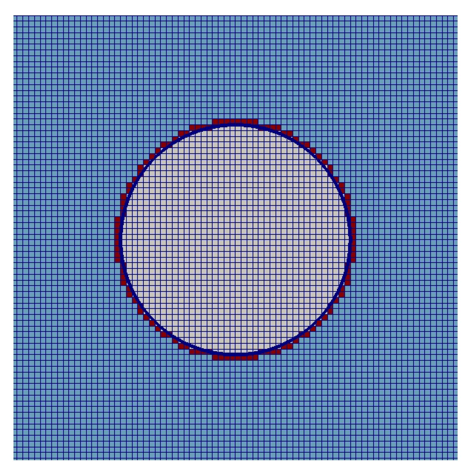
The IBM developed in our previous work [22] is adopted for the calculation of the body force term $\mathbf{f}$ in the momentum equation. The first step is to divide into three domains with respect to the IB surface $\mathcal{S}$, which are the solid domain, forcing domain and the fluid domain. The resultant computation domain for a circular boundary is shown in Figure 1 as an example.

The body force term $\mathbf{f}$ will then be imposed in the forcing and solid domains to represent the proper boundary conditions on the IB surface. Similar to the method for single-phase flows, $\mathbf{f}$ is calculated by:

$$\mathbf{f}=\frac{\partial \rho {\mathbf{u}}^{*}}{\partial t}+\nabla ·\left(\rho {\mathbf{u}}^{*}{\mathbf{u}}^{*}\right)-\nabla ·\left[\rho {\nu }_{\mathrm{eff}}\left(\nabla {\mathbf{u}}^{*}-\nabla {{\mathbf{u}}^{*}}^T\right)\right]+\nabla p_{\mathrm{rgh}}+\mathbf{g}·\mathbf{x}\nabla \rho$$

(10)

where,

$${\mathbf{u}}^{*}=\left\{\begin{array}{cc}\mathcal{L}\left(\mathbf{u}\right),\hfill & \mathrm{forcing}\mathrm{domain}\hfill \\ {\mathbf{u}}_{\mathrm{body}},\hfill & \mathrm{solid}\mathrm{domain}\hfill \end{array}\right.$$

(11)

in which, the operator $\mathcal{L}(*)$ denotes the interpolation of the velocity near the IB surface. The interpolation is based on the solution of the governing equations and the velocity boundary conditions on the IB surface. The second-order Laplacian interpolation is used in the present work. The detailed descriptions and a series of verification and validation tests can be found in [22].

Different from the IBM used in the single-phase flow, the additional gradient of density in the momentum equation due to buoyancy is challenging for the IBM. Since the fluid inside the solid domain is unphysical, the volume fraction $\alpha$ and the density field are not properly determined at this stage. By examining Equation (9), one can find that without a proper setup of the volume fraction $\alpha$ near the IB surface, the calculation of the density field is problematic in that region. In addition, considering the density ratio between air and water, large error will be introduced to the calculation of the gradient of density near the IB surface, leading to an incorrect solution of the momentum equation.

In the current work, the dilation method proposed by Sun and Sakai [19] is adopted. At the end of each time step, the volume fraction field is extended into the solid domain as follows:

• Mark all solid cells and store in a list $\mathcal{M}$.
• Loop through all marked cells in $\mathcal{M}$.

  (a)

  Check all the cells that share nodes with the marked cell i, and store the indices of all unmarked cells. The volume fraction $\alpha$ of these cells is used to interpolate the $\alpha$ in cell i.

  (b)

  After storing all the unmarked cells, use the inverse square distance method to interpolate ${\alpha }_i$ as

  $${\alpha }_i=\frac{{\sum }_j{w}_j{\alpha }_j}{{\sum }_j{w}_j}$$

  (12)

  where

  $$w_j=\frac{1}{d^2}$$

  (13)

  where d is the distance between the cell centers of i and j. j is the cell index of each unmarked cell.

  (c)

  Store the cell index i into a temporary list $\mathcal{S}$.

  (d)

  Go to next marked cell $i+1$.

• Remove all cells in $\mathcal{S}$ from $\mathcal{M}$.
• Go back to the beginning of Step. 2.

The number of iterations in Step. 2 determines how many layers of solid cells $\alpha$ are extended inside the IB surface. Note that this extension is naturally a good approximation of the Neumann boundary condition. In practice, we find that five layers are good enough for both cases with both static and moving IB surfaces. It should be noted that this process of extension changes the fluid volume in the solid domain solely to enforce the Neumann boundary condition of $\alpha$ on the IB. Therefore, it changes the total fluid volume in the whole domain. However, since the velocity boundary condition is imposed on the IB, there is no velocity flux across the IB boundaries. Change of the fluid volume in the solid domain serves the sole purpose to impose the correct boundary condition of $\alpha$ on the IB, and does not affect the total volume in the fluid domain.

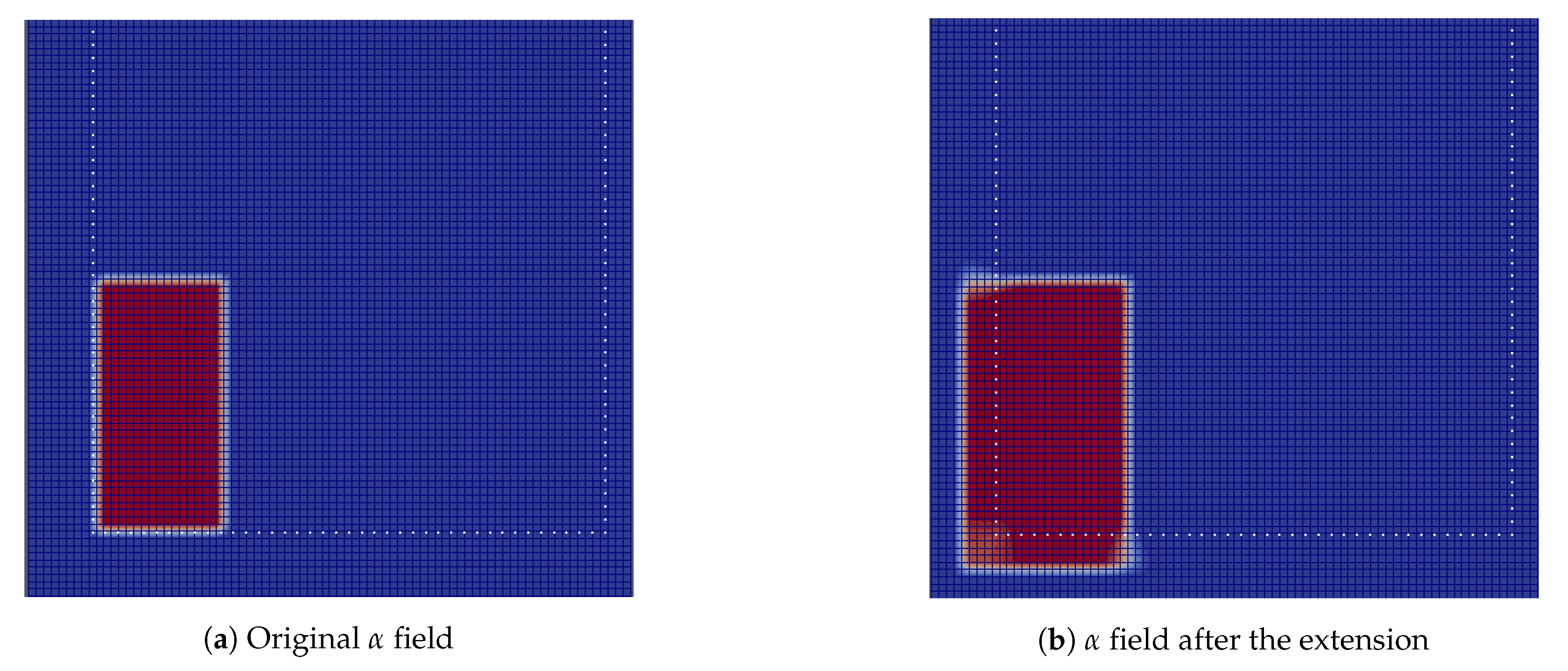
The effect of the field extension operation is demonstrated by the canonical 2D dam-break problem. In this case, the dam walls are modeled using IB surfaces, which do not coincide with the grid lines, as shown in Figure 2a. In Figure 2, the color represents the value of the volume fraction $\alpha$, where red represents water $\alpha =1$, and blue represents air $\alpha =0$. The IB surfaces are denoted as white dots.

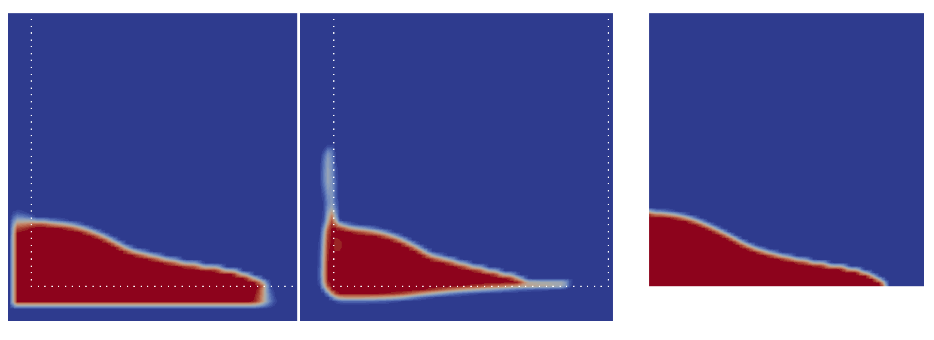
Figure 3 shows the comparison of the shape of the air–water interface between the present IBM and the results on the body-fitted mesh with the same mesh resolution after the dam is released. The shape of the air–water interface, especially at the water front along the tank bottom, is not correctly predicted without the field extension. Inaccurate simulation of the water volume will cause a poor prediction of the momentum of the water body, leading to an inaccurate simulation of the development of fluid field and the impact force.

2.4. Turbulence Modelling

Following our previous work [22], the Spalart–Allmaras turbulence model is used in the current work. Previous results of flows in an asymmetric diffuser and behind a KVLCC2 ship model demonstrate that moderate flow separation can be well handled with decent accuracy. It should be noted that for many marine hydrodynamic applications where massive separation effects are important, more advanced turbulence modelling techniques can offer additional accuracy, such as DES or LES.

In the Spalart–Allmaras turbulence model, the turbulent viscosity ${\nu }_t$ is calculated by solving the transport equation of the modified turbulent viscosity $\tilde{\nu }$:

$$\begin{array}{cc}\hfill \frac{D}{Dt}\tilde{\nu }=& \frac{1}{{\sigma }_{{\nu }_t}}\nabla ·((\nu +\tilde{\nu })\nabla \tilde{\nu })+\frac{C_{b2}}{{\sigma }_{{\nu }_t}}{|\nabla \tilde{\nu }|}^2+C_{b1}\tilde{S}\tilde{\nu }(1-f_{t2})\hfill \\ \hfill & -(C_{w1}{f}_w-\frac{C_{b1}}{{\kappa }^2}{f}_{t2})\frac{{\tilde{\nu }}^2}{{\tilde{d}}^2}+S_{\tilde{\nu }}\hfill \end{array}$$

(14)

with the wall boundary condition ${\tilde{\nu }}_{\mathrm{wall}}=0$. Detailed description of the model and the default model coefficients can be found in [23]. The near-wall distance $\tilde{d}$, which is essential for the correct modelling of the destruction of the turbulence, is calculated taking into account the IB surfaces. As proposed in our previous work, the IB wall function is also used to relax the requirement of the near-wall cell spacing. The wall function provides a universal velocity profile from the outer edge of the logarithmic layer down to the IB surface. The wall tangential component of the velocity in the forcing cell is corrected based on the velocity profile. $\tilde{\nu }$ in the forcing cell is directly calculated based on a linear profile as follows:

$${\tilde{\nu }}^{+}=\kappa y^{+}$$

(15)

in which ${\tilde{\nu }}^{+}=\tilde{\nu }/\nu$; $\kappa =0.41$ is the Von Karman constant; $y^{+}=y{u}_{\tau }/\nu$; $u_{\tau }$ is the friction velocity determined from the Spalding’s velocity profile:

$$y^{+}=u^{+}+\frac{1}{E}\left[e^{\kappa u^{+}}-1-\kappa u^{+}-\frac{1}{2}{\left(\kappa u^{+}\right)}^2-\frac{1}{6}{\left(\kappa u^{+}\right)}^3\right]$$

(16)

3. Numerical Results

3.1. 3D Dam-Break with an Obstacle

In this section, the canonical problems of dam-break are investigated. Two different setups are considered to validate the solver from different aspects including the flow velocity, development of the air–water interface and the impact on the obstacle.

3.1.1. Dam-Break No.1

This section discusses the interaction between a vertical square cylinder and a single large wave caused by the dam break. The flow velocity in front of the obstacle and the impact force on the square cylinder are examined. The experimental data is found in [24] provided by Profs. Catherine Petroff and Harry Yeh. Numerical results are also provided in [24] using their three-dimensional Eulerian-Lagrangian marker and micro-cell method.

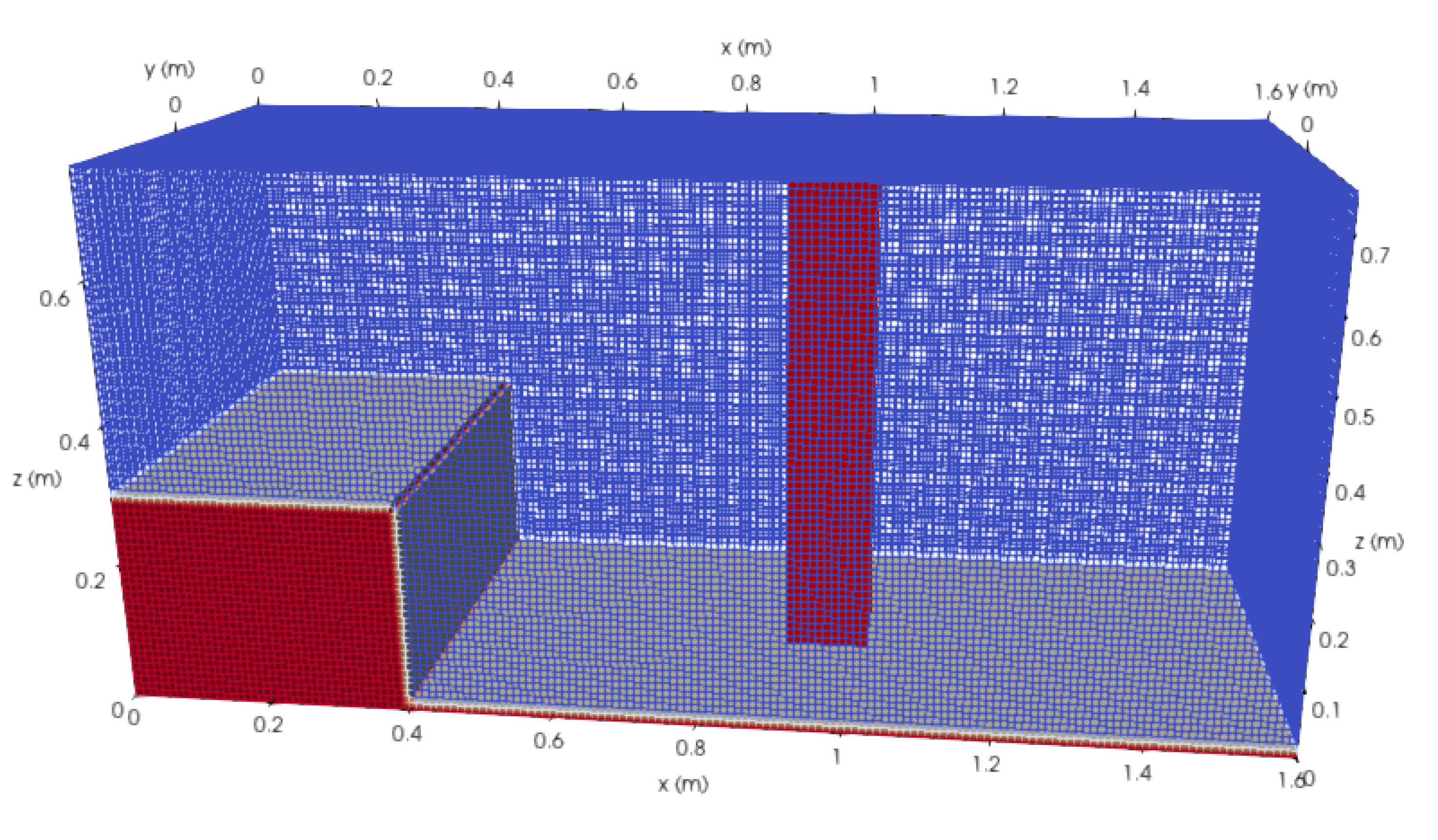
Figure 4 illustrates the setup of the numerical simulation. The dimensions of the tank are $1.6\mathrm{m}\times 0.61\mathrm{m}\times 0.75\mathrm{m}$. A volume of water with the size $0.4\mathrm{m}\times 0.61\mathrm{m}\times 0.3\mathrm{m}$ is initially placed at the left end of the tank. The dimensions of the vertical obstacle are $0.12\mathrm{m}\times 0.12\mathrm{m}\times 0.75\mathrm{m}$. It is placed downstream of the volume of water with center of the bottom of the obstacle at $(0.96,0,0)$. As reported by Petroff and Yeh, the bottom of the tank was not completely drained in the physical experiment. Therefore, a thin layer of water with $0.01\mathrm{m}$ in depth is setup in the present simulation as shown in Figure 4.

It should be noted the way that the water is released in the present simulation is different from how the experiment was conducted. In the physical experiment, the water is blocked by a gate that is lifted vertically with finite speed at the beginning of the test, whereas in the simulation the water is released instantaneously. Lin and Chen [25] discuss the influence of the opening speed of the gate on the time history of the impact force on the obstacle. Their results show that the peak of the impact force is delayed as the finite opening speed of the gate decreases.

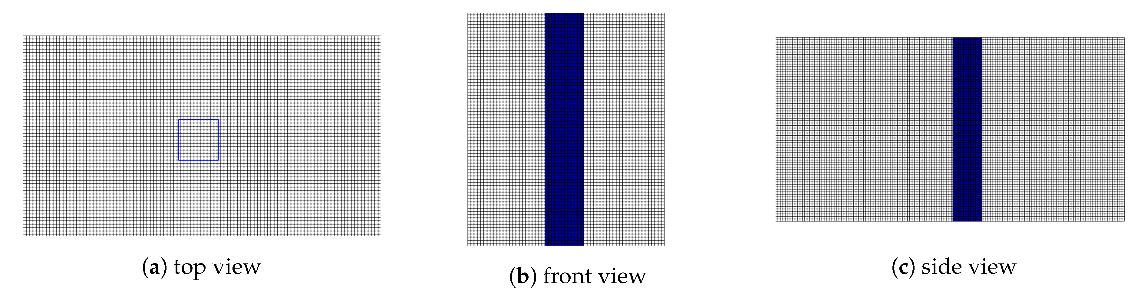
In the present simulations, the walls of the tank are represented by the body-fitted wall boundaries as shown in Figure 4. The solid walls of the vertical obstacle are represented by an IB surface. A set of three background meshes with a refinement ratio of $\sqrt{2}$ in each direction is used to validate the solver. The total numbers of cells of the background meshes are $114\times 43\times 53$, $161\times 61\times 75$ and $228\times 86\times 106$, respectively. The position of the IB in the tank is shown in Figure 5.

The density and viscosity are ${\rho }_w=1000\mathrm{kg}/{\mathrm{m}}^3$, ${\nu }_w=1\times {10}^{-6}{\mathrm{m}}^2/\mathrm{s}$ for the water, and ${\rho }_a=1\mathrm{kg}/{\mathrm{m}}^3$, ${\nu }_a=1\times {10}^{-5}{\mathrm{m}}^2/\mathrm{s}$ for the air. The gravitational acceleration is $g=9.81\mathrm{m}/{\mathrm{s}}^2$. In the simulations, the time step size is adjusted automatically to keep the Courant number less than 1.0.

A probe is used to record the flow velocity at a location in front of the obstacle at $(0.754,0,0.026)$. In addition, the impact force on the obstacle is calculated.

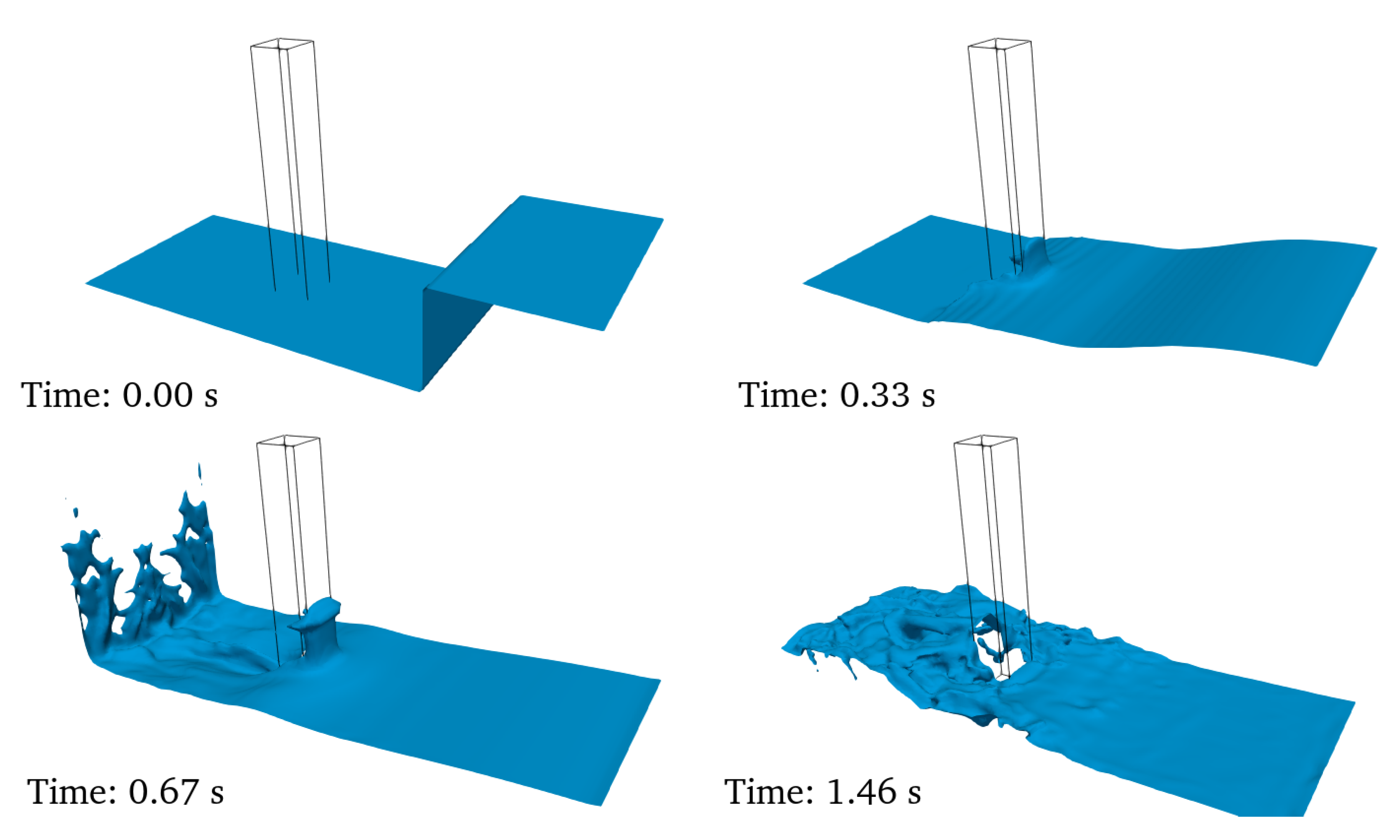
Figure 6 shows the wave propagation and its interaction with the obstacle at different time instants. It provides a general idea of what the critical phases of the dam-break problem look like. At $t=0$ s, the water is released. After the water hits the front side of the obstacle, it runs up along the front wall and causes a large impact force. Afterwards, the water that travels around the obstacle joins together behind the obstacle, travels to the end of the tank, and hits the back side of the obstacle after being reflected by the end wall of the tank. It causes a second impact in the opposite direction compared to the first peak of impact. The second impact force is expected to be weaker than the first one because the velocity of the front of the wave is decreasing in general.

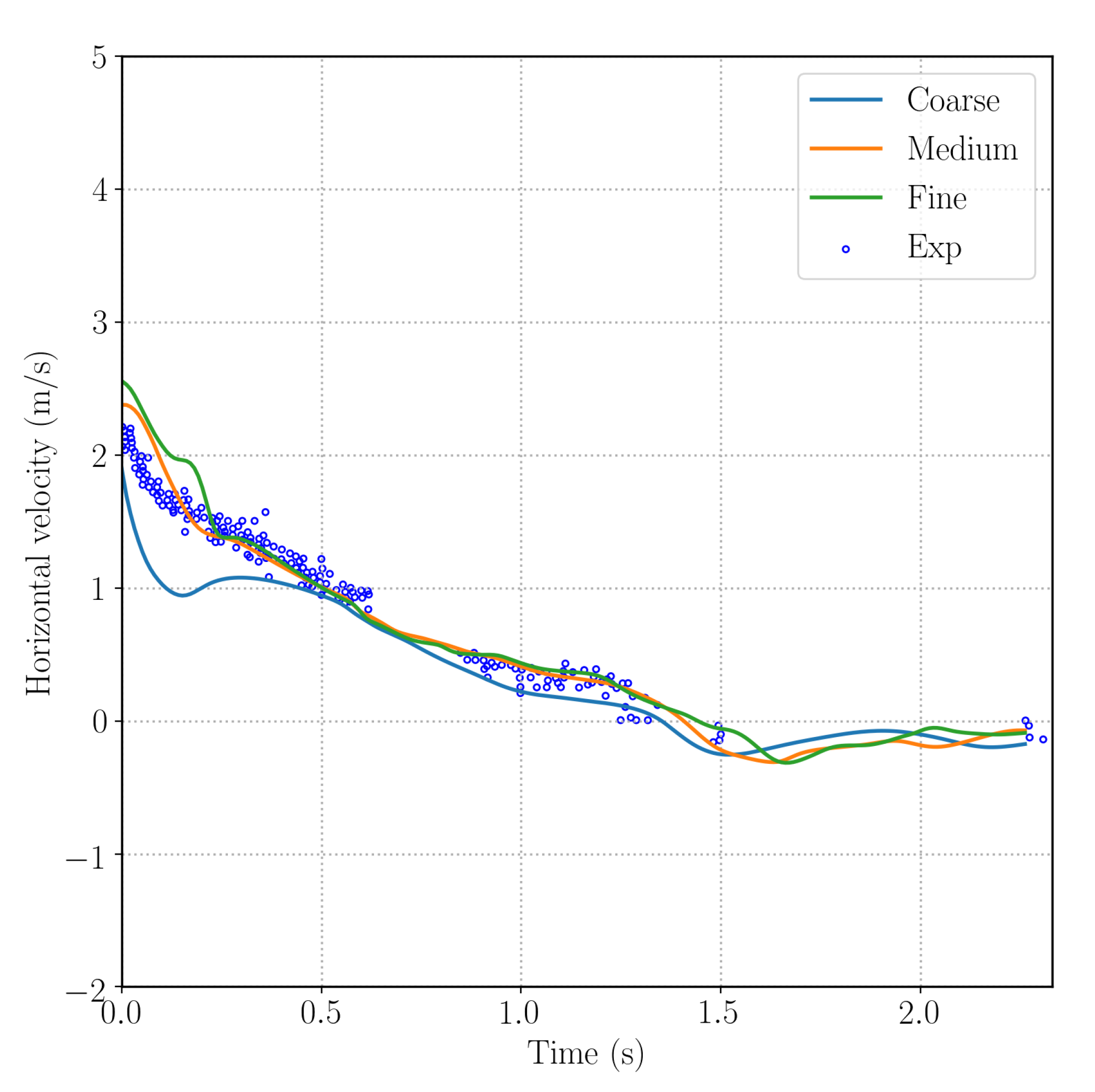
To further evaluate the accuracy of the solver, Figure 7 shows the x-component of the velocity at the velocity probe using all three background meshes. The data is shifted in time such that $t=0$ s in the figure is the moment when the water first reaches the probe. Specifically, $t=0\mathrm{s}$ in the figure corresponds to $0.238$ s after the water is released. The experimental data is plotted together for the purpose of comparison. The gaps in the experimental data at $0.6<t<0.85$ s and $t>1.5$ s are due to the presence of bubbles in the water as explained in [24]. The velocity at $t=0\mathrm{s}$ is slightly overpredicted by the medium and fine meshes, which means the water moves faster in present simulations than in the experiment. It should be noted that in the simulations, the floor is set to be covered by a thin layer of water of thickness $0.01\mathrm{m}$. The layer of water is used to mimic the wet floor in the experiment. However it cannot perfectly reproduce the experimental environment. Another reason is that the gate in front of the water is released with finite speed in the experiment, which reduces the velocity at the water front near the floor. A similar conclusion is drawn in [25] by investigating the influence of the release speed of the gate. The medium and fine meshes correctly predict the decrease in the velocity of the water (e.g., $0<t<1.5\mathrm{s}$) due to the blockage of the obstacle. After $t=1.5\mathrm{s}$, the wave is reflected from the tank wall at $x=1.6\mathrm{m}$, and it is further blocked by the back side of the obstacle. The water near the bottom floor in front of the obstacle is almost stationary. This can be confirmed from Figure 7 that the velocity at the probe drops to almost zero after $t=1.5\mathrm{s}$.

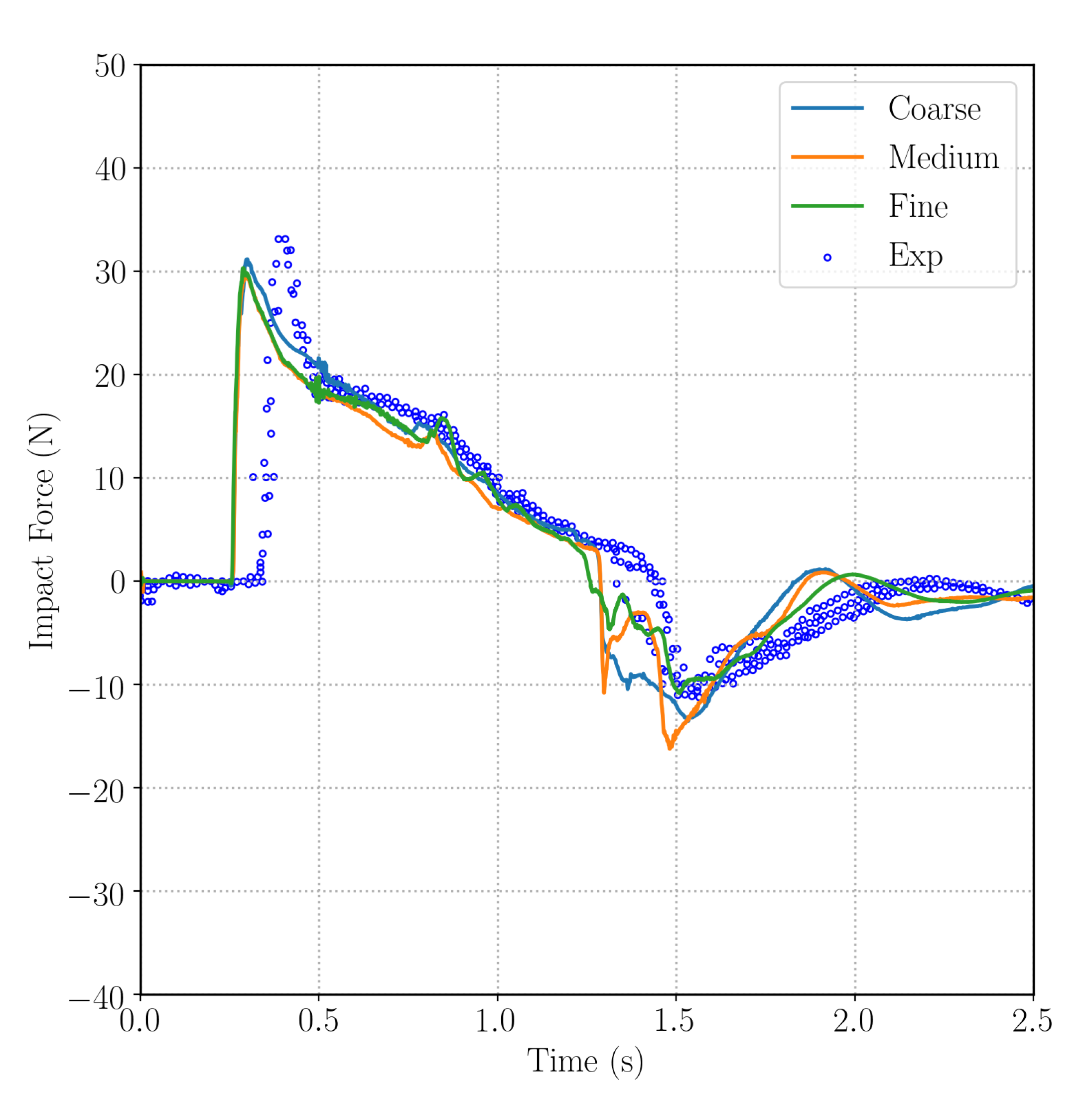
Figure 8 shows the impact force on the obstacle. It is worth pointing out that $t=0\mathrm{s}$ in this figure corresponding to the time when the simulation starts, which explains the zero impact force at about $t<0.25\mathrm{s}$. The different background meshes predict a consistent start time of the impact. Compared with the experimental data, it can be seen that the first impact happens earlier than in the experiment, which is consistent to the behavior of the horizontal velocity at the velocity probe discussed before. Figure 8 shows that the numerical results slightly underpredict the positive peak value at around $t=0.4\mathrm{s}$. Afterwards, the impact force decreases gradually to zero around $0.4<t<1.5\mathrm{s}$, which is consistent with experimental data. At $t\approx 1.5\mathrm{s}$, the wave reflected from the end the tank arrives and impacts on the back side of the obstacle causing a negative peak of the impact force. During the last phase of the dam break, the impact force decreases to zero again.

In summary, the accuracy of the solver is demonstrated via the comparisons between the numerical solutions and the experimental data for the impact force and the horizontal velocity in the front of the obstacle.

3.1.2. Dam-Break No.2

In the previous section, the discussion is focused on the velocity of the water and the total impact force, which is an integrated variable. It is equally important to investigate the local pressure during the impact, as well as the water elevation at different places. To fulfill this goal, a different setup of the 3D dam-break problem with an obstacle is used in this section. The height of the obstacle is much smaller than in the previous case, which means the water also flows over the top of the obstacle. The physical experiment was carried out by the Maritime Research Institute Netherlands (MARIN, [26]) to investigate the phenomenon of green water on the deck of a ship. Local pressure at different positions of the obstacle, and the water elevation at different locations of the tank were recorded in the experiment. The results of numerical simulations are also provided in [26].

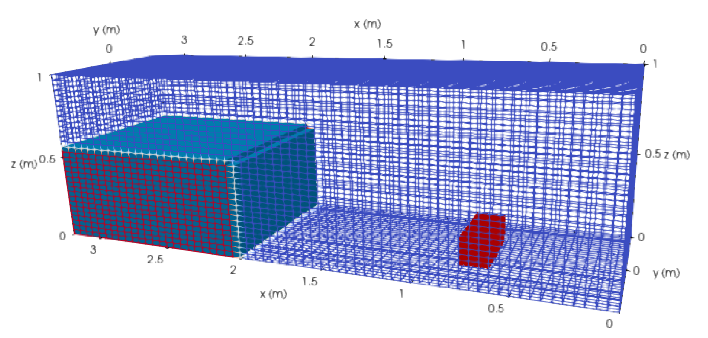
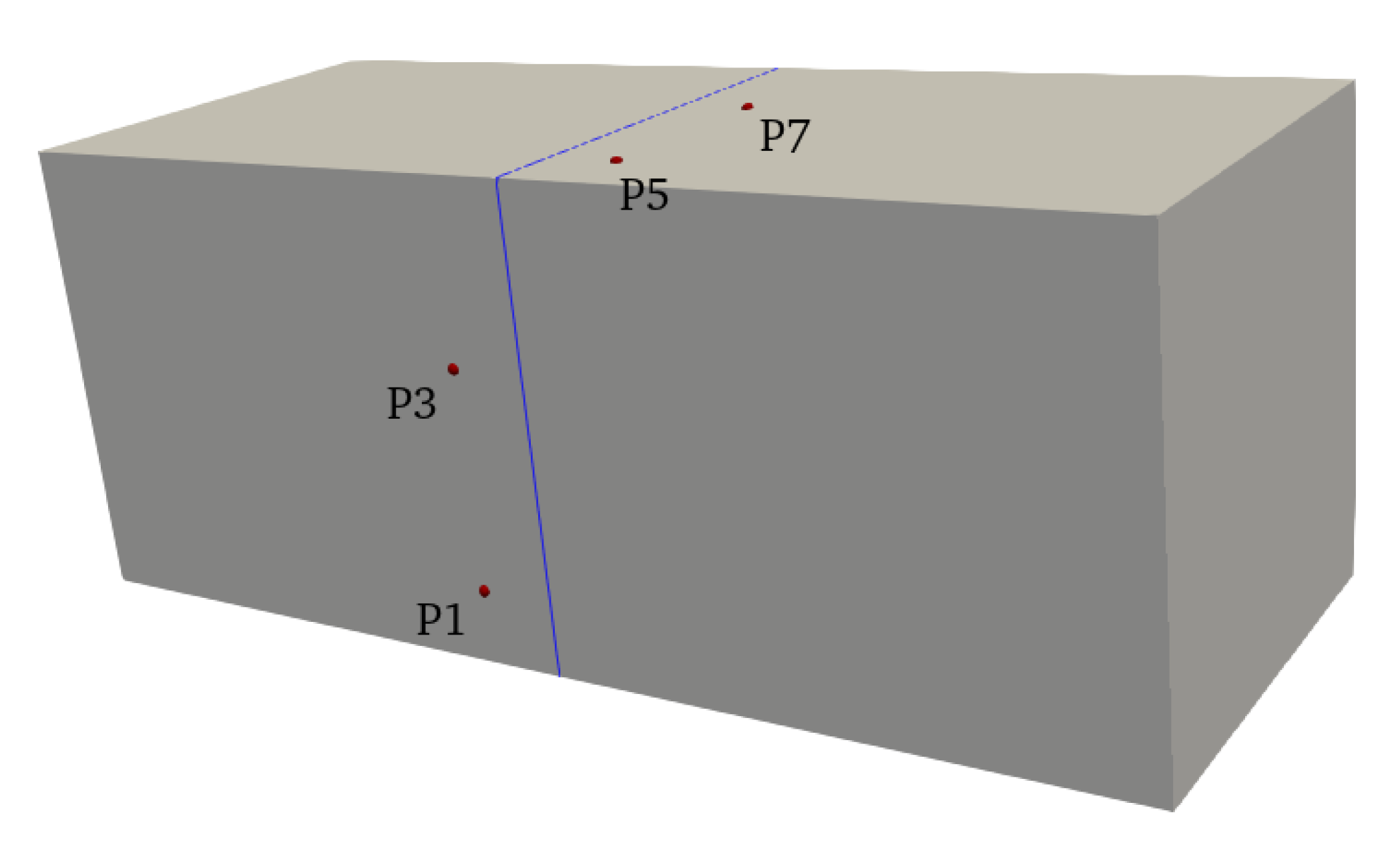
Figure 9 shows the computational domain and the numerical setup. The dimensions of the tank are $3.22\mathrm{m}\times 1\mathrm{m}\times 1\mathrm{m}$. At the beginning of the simulation, the volume of water with the size $1.22\mathrm{m}\times 1\mathrm{m}\times 0.55\mathrm{m}$ is located at the end of the tank from $x=2\mathrm{m}$. A rectangular obstacle is placed in front of the dam to represent a container on the deck of the ship. The dimensions of the obstacle are $0.16\mathrm{m}\times 0.4\mathrm{m}\times 0.16\mathrm{m}$ with its front side (the side which faces the dam) positioned at $x=0.83\mathrm{m}$. The water elevation is monitored at two places along the vertical plane $y=0\mathrm{m}$, which are $x=1.0\mathrm{m}$ and $2.66\mathrm{m}$. Eight sensors are used to record the local pressure on the top and front sides of the obstacle, and the locations are listed in

Table 1. Locations of the pressure sensors in the 3D dam-break problem No.2.

Sensor	Location
P1	$(0.83,-0.026,0.025)$
P2	$(0.83,-0.026,0.063)$
P3	$(0.83,-0.026,0.099)$
P4	$(0.83,-0.026,0.136)$
P5	$(0.806,0.026,0.16)$
P6	$(0.769,0.026,0.16)$
P7	$(0.733,0.026,0.16)$
P8	$(0.696,0.026,0.16)$

. The numerical results of the time histories at the pressure sensors P1, P3, P5 and P7 are compared with the experimental data. The locations of these four sensors are illustrated in Figure 10. The sensors P1 and P3 are on the side facing to the initial volume of water. The blue solid line represents the plane $y=0\mathrm{m}$ as a reference.

The density and viscosity of the water are ${\rho }_w=998.2\mathrm{kg}/{\mathrm{m}}^3$, ${\nu }_w=1\times {10}^{-6}{\mathrm{m}}^2/\mathrm{s}$, and ${\rho }_a=1\mathrm{kg}/{\mathrm{m}}^3$, ${\nu }_a=1.48\times {10}^{-5}{\mathrm{m}}^2/\mathrm{s}$ for the air. The gravitational acceleration is $g=9.81\mathrm{m}/{\mathrm{s}}^2$. Similar to the previous section, a set of three background meshes with a refinement ratio of $\sqrt{2}$ in each direction is used. The number of cells of the background meshes are $64\times 32\times 32$, $90\times 46\times 46$ and $128\times 64\times 64$, respectively. All the sides of the tank are represented by the body-fitted boundary conditions as no-slip walls, and the obstacle is modeled with an IB. The time step size is adjusted automatically to keep the global Courant number less than 0.75 and the Courant number near the free surface less than 0.3.

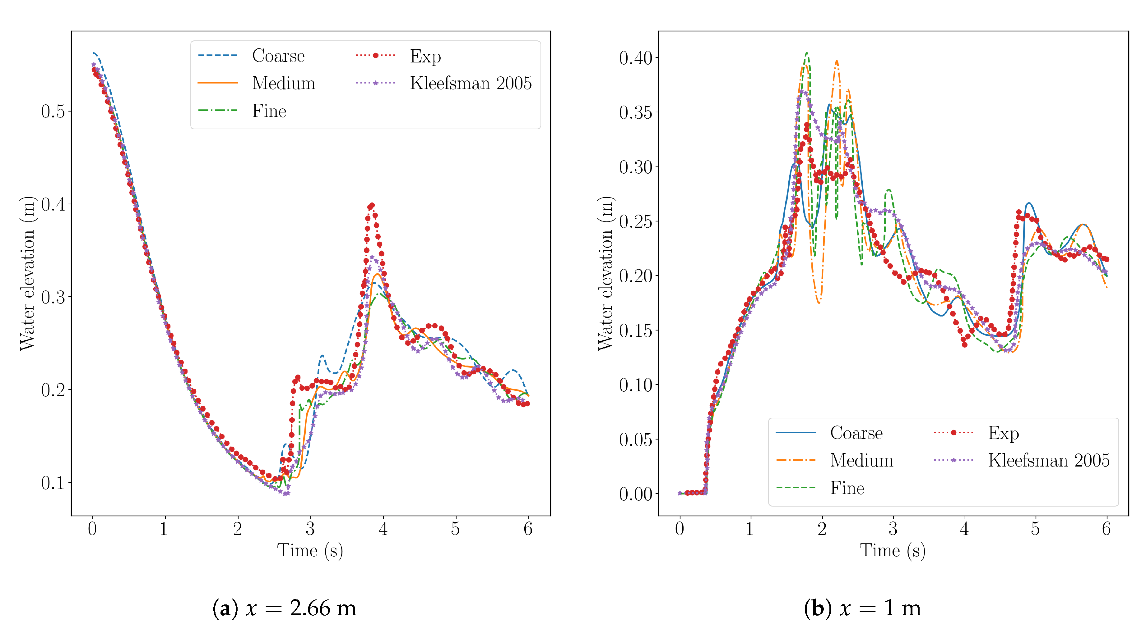
Figure 11 shows the time histories of the water elevation at the locations $x=2.66\mathrm{m}$ and $1.0\mathrm{m}$, which are inside the initial position of the dam and in front of the obstacle, respectively. During the initial part of the time series the comparison between the experiment and simulation is very close. At about $t=2.5\mathrm{s}$ and $1.8\mathrm{s}$, the water reflected from the wall of the tank at $x=0\mathrm{m}$ arrives to the two probes, and causes a random unsteady and high frequency response. For the second part of the time histories, there are differences between the numerical results and the experimental data with regard to the high frequency part, yet the mean elevation is in very close agreement. For example in the probe at $x=1\mathrm{m}$, the front of the water arrives at around $t=4.5$ s, and the numerical results accurately capture the instant when the air–water interface starts to rise in accordance with the experiments.

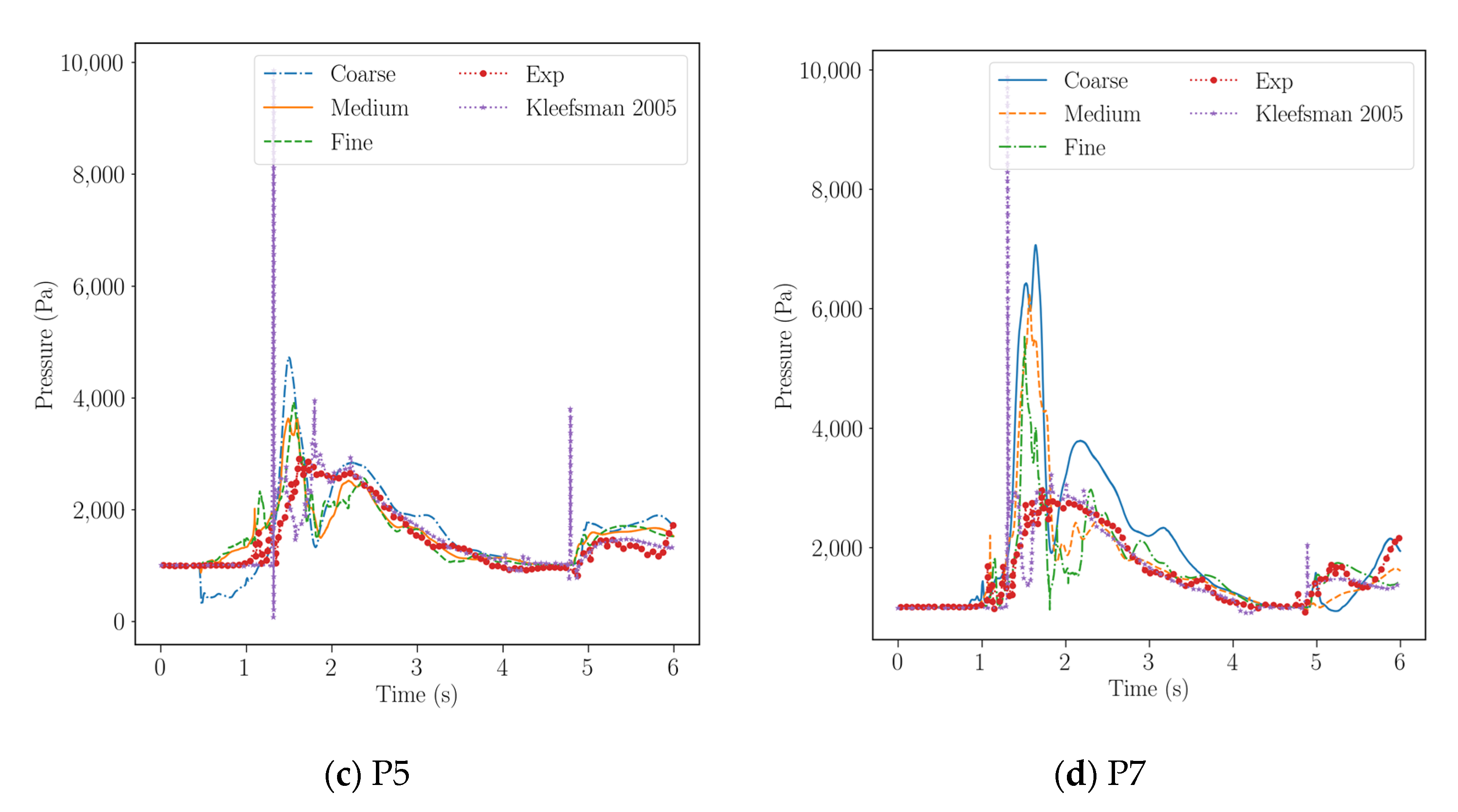
As shown in Figure 12, the time histories of the local pressure at four different sensors are selected to compare with the experimental data. The present numerical simulation captures the behavior when the water first impacts the sensors, especially for the ones on the front side of obstacle. The peak pressure at P1 matches with the experimental data very well, while the peak pressure at P3 is underpredicted by the fine mesh. At around $2<t<4\mathrm{s}$, the pressure at both sensors drops gradually.

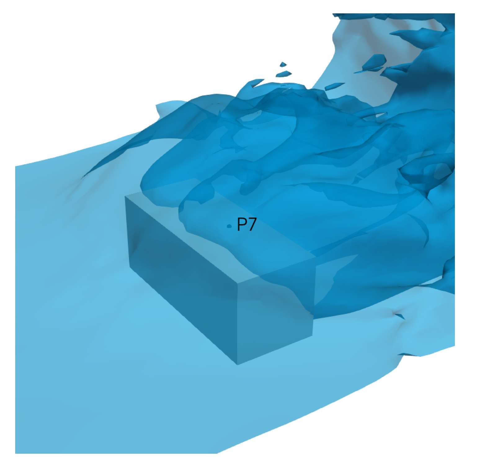
For the numerical results at P5 and P7, which are on the top surface of the obstacle, the numerical results show a large oscillation. It is because when the water flow over the obstacle, the large vertical velocity of the water causes the water to detach from the surface of the obstacle. Subsequently, air is entrapped when the water starts to impact on the top the obstacle. However, the effect of air compressibility is not considered in the current solver. Figure 13 shows the profile of the air–water interface around the pressure sensor P7 at around $t=1.1\mathrm{s}$. It can be clearly seen that the air is entrapped and a bubble is formed around P7. As a result, the large oscillation appears in the numerical results at P5 and P7 in the limitations of the current numerical framework.

Overall, the results demonstrate that the present IBM solver can handle the problems of wave interaction with solid walls with respect to the evolution of the air–water interface, velocity of the water, force on the obstacle and the local pressure due to the impact.

3.2. Water Exit of a Circular Cylinder

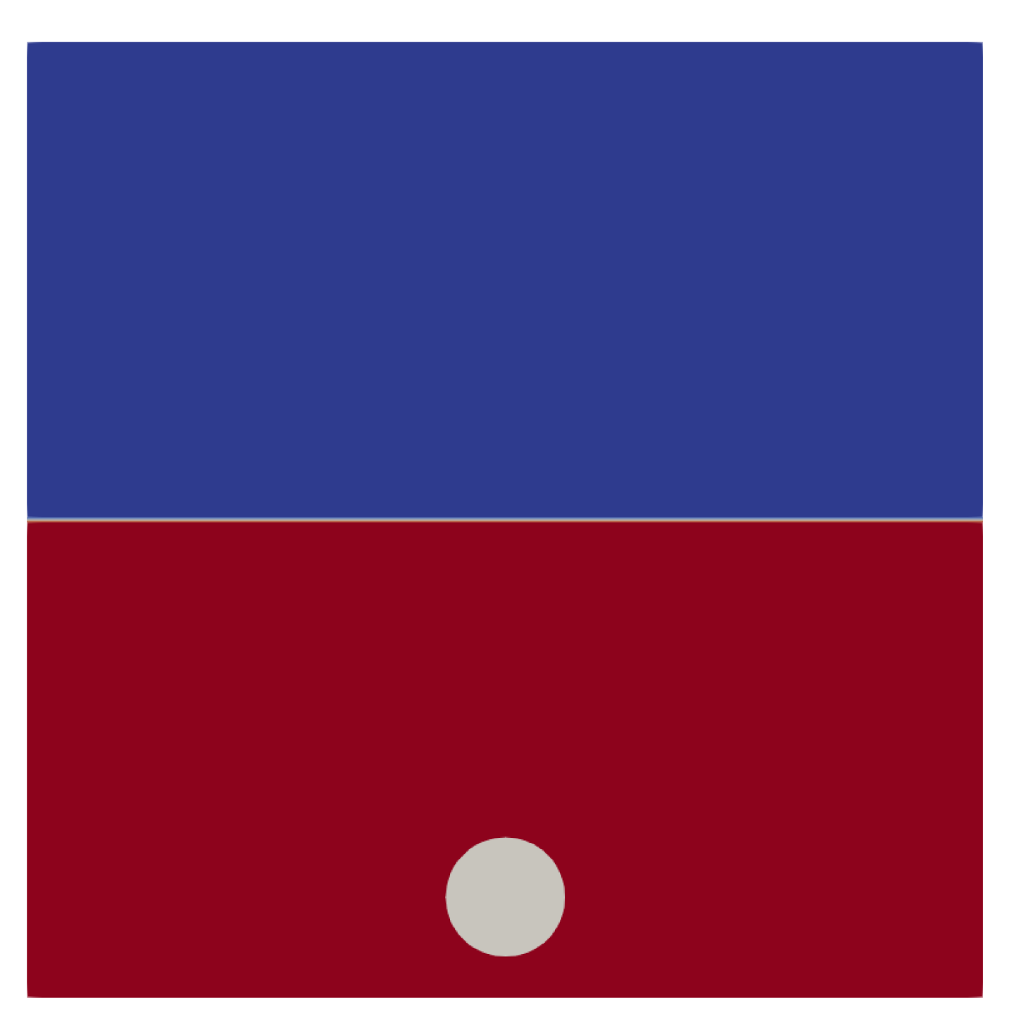
In this section, the IBM is used to simulate a moving surface in the air–water two-phase flow to further demonstrate its capability. The test case is the water exit of a 2D circular cylinder with constant vertical velocity. The physical experiments were conducted by Miao [27]. The results of the numerical simulations carried out by Zhu et al. [28] are also presented as a reference. The numerical simulations use the Constrained Interpolation Profile (CIP) method.

The computational domain and the initial position of the cylinder with the radius of $R=0.0625\mathrm{m}$ are shown in Figure 14. The domain is $1\mathrm{m}$ wide and the water depth is $h=0.5\mathrm{m}$. At the beginning of the simulation, the cylinder accelerates upwards from rest and gradually reaches the final constant velocity v. Eventually, the cylinder exits the water until the water fully dropped from the surface the cylinder. In the present simulations, the cylinder is represented using the IB, and a uniform structured mesh is used as the background mesh with the cell size $\Delta x=\Delta y=0.04R$.

In the experiment, the dimensionless time $vt/R=0$ corresponds to the time instant when the top of the cylinder touches the air–water interface. $vt/R=-5.5$ and $-5$ correspond to the time instants where the cylinder starts to move and reaches the final velocity v, respectively. The prescribed motion of the cylinder is described by the position of the center of the cylinder with respect to time:

$$y\left(t\right)=\left\{\begin{array}{cc}\frac{1}{2}v(t-\frac{t_0}{\pi }sin\left(\frac{\pi t}{t_0}\right)),\hfill & t<t_0\hfill \\ v(t-\frac{1}{2}{t}_0),\hfill & t\ge t_0\hfill \end{array}\right.$$

(17)

where $t_0$ is the time of ramping up the velocity. It should be noted that in the simulations, $t=0\mathrm{s}$ corresponds to the time instant when the cylinder starts to move.

Two numerical tests are carried out with different final velocity v as listed in

Table 2. Parameters for the water exit tests.

Test	$\mathbf{Fr}$	$\mathit{v}\left(\mathbf{m}/\mathbf{s}\right)$	${\mathit{t}}_0\left(\mathbf{s}\right)$
No.1	0.4627	0.5124	0.0610
No.2	0.6903	0.7644	0.0409

.

The time step size is automatically adjusted to keep the global Courant number less than 1.0 and the Courant number near the free surface less than 0.3.

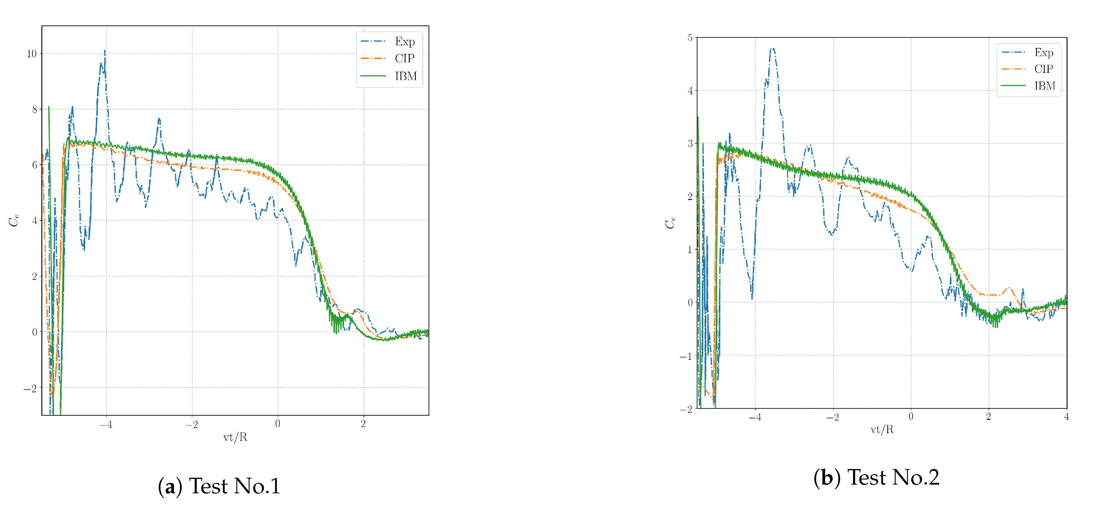
Figure 15 shows the time histories of the exit coefficient $C_e$ for the two test cases. The time $t=0$ of the present simulations is shifted to compare with the experimental data. The exit coefficient $C_e$ is defined as:

$$C_e=\frac{F}{\rho v^{2}R}$$

(18)

where $\rho$ is the density of water and F is the vertical hydrodynamic force on the cylinder.

For both test cases, the present numerical results show good agreement with the experimental data. In general, $C_e$ shows similar trend for both exit speeds. Before the dimensionless time $vt/R<-5$, the cylinder starts to accelerate from its initial position. It results in a large negative peak in force, which is captured by all the three results for both cases. For the time range $-5<vt/R<0$, the cylinder moves upward with a constant speed. As the cylinder approaches the surface of the water, $C_e$ gradually decreases with a nearly constant rate of change. In addition, the vertical speed of the cylinder does not have much influence on the rate of decrease of $C_e$. When the cylinder starts to exit from the water at $vt/R=0$, the hydrodynamic force drops significantly, and eventually becomes zero when the cylinder is drained after it completely leaves the water.

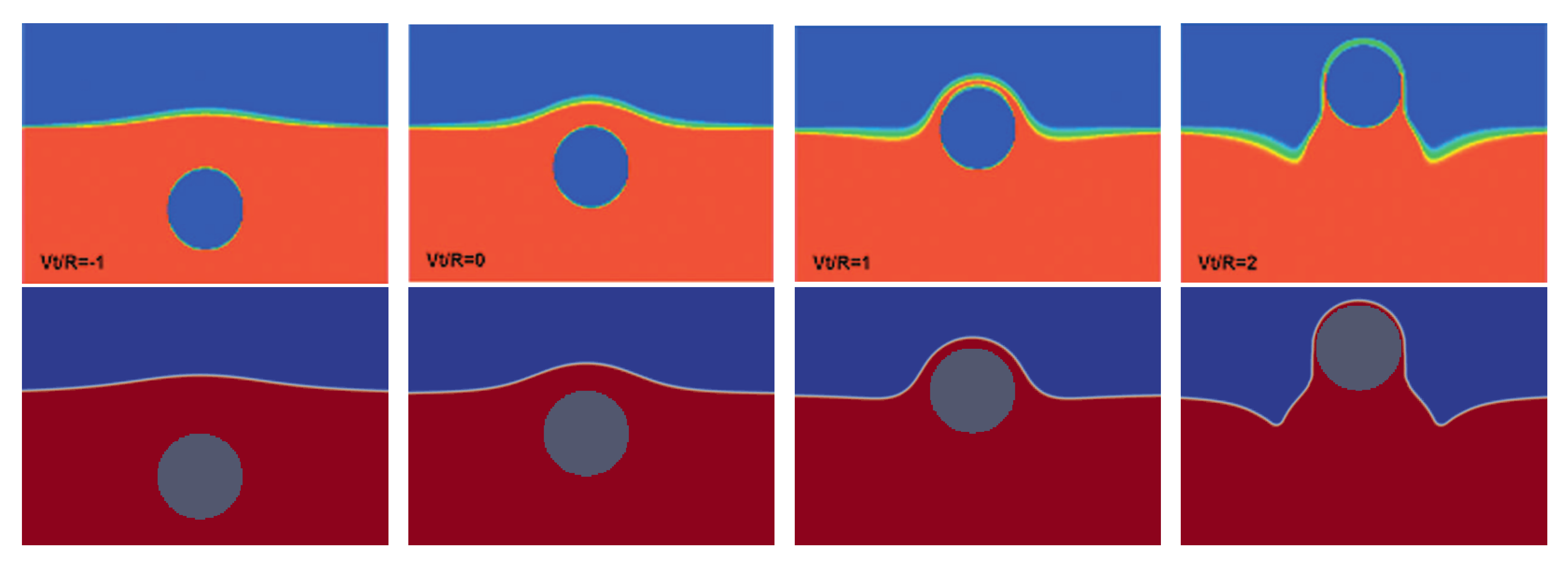
Figure 16 shows the comparison of the profile of the air–water interface with the numerical solutions of Zhu et al. [28] at different time instants. The present results show overall good agreement with the other numerical results with respect to the hydrodynamic force on the cylinder with different exit velocities. When the cylinder exits the water after $vt/R=0$, the present results capture the thin layer of water on top of the cylinder. The present results also predict the deformation of the air–water interface when the layer of water starts to fall down along the surface of the cylinder at $vt/R>1$.

In summary, for both vertical speeds of the cylinder, the present IBM quantitatively captures the unsteady behavior of the hydrodynamic force at different phases of the two water-exit tests. In addition, the deformation of the air–water interface, especially due to the interaction between the IB surface and the air–water interface is accurately modeled.

3.3. KCS Model Advancing with a Rotating Rudder

To fully demonstrate the flexibility and the accuracy the present IBM. A combined usage of IB surfaces and unstructured body-fitted approach is considered in this section, which is a KCS ship model advancing with a rotating rudder. More specifically, the computational domain is drawn using unstructured mesh with body-fitted boundary on the ship hull and the fixed rudder horn. The rotating rudder blade is modeled using an IB surface.

In this simulation, the equations are written in a coordinate system that moves with the constant velocity of the ship hull. In addition, the boundary layer flow is more well defined on the ship hull than in the wake where the rudder operates, due the high Reynolds number. For such a case, using an unstructured grid and body-fitted approach on the ship hull is more efficient than IBMs. If an IB is used to represent the entire ship hull, it will require many more cells to achieve similar accuracy since it requires resolution in the boundary layer cells in all directions. Whereas, if the body-fitted approach is applied to the rotating rudder blade, a huge amount of time and effect is required to properly design the mesh to achieve satisfying mesh quality near the tip of the blade, and in the gap between the blade and the rudder horn. Additional attention is also required to design the mesh topology such that the mesh quality is preserved due to the rotation of the blade. In comparison, using an IB to represent the rotating rudder blade completely avoids mesh motion and also saves the effort of designing the mesh. A novel capability of our approach is to combine the benefits of unstructured grid, body-fitted approach and an IBM Therefore, the present IBM, which can be used together with body-fitted boundaries on unstructured grids, is more flexible and efficient than other IBMs, where all boundaries are represented by IBs and structured background grids are used.

The ship model and the rudder are shown in Figure 17. in which, the propeller is not considered. The main particulars of the model-scaled KCS and the rudder are listed in

Table 3. Main Particulars of the model-scaled KCS.

Main Particulars	Symbol	Value
Scale	$\lambda$	105
Length between perpendiculars	$L_{\mathrm{pp}}\left(m\right)$	2.19
Length of waterline	$L_{\mathrm{wl}}\left(m\right)$	2.2143
Width	$B_{\mathrm{wl}}\left(m\right)$	0.3067
Depth	$D\left(m\right)$	0.1810
Draft	$T\left(m\right)$	0.1029
Displacement	$\Delta$(m${}^3)$	0.0449
Wetted area without rudder	S(m${}^2)$	0.8644
Longitudinal center of buoyancy (fwd+)	LCB $(\%L_{\mathrm{pp}})$	–1.48
Vertical center of gravity	KG (m)	0.118
Moment of inertia	$K_{\mathrm{yy}}/L_{\mathrm{pp}}$	0.25

and

Table 4. Main Particulars of the model-scaled rudder.

Main Particulars	Value
Scale	105
Type	Semi-balanced horn rudder
Area of rudder (m${}^2$)	0.0104
Lateral Area of rudder (m${}^2$)	0.0049

, respectively.

In the simulations, the ship model is fixed in the even-keel condition without considering the vertical motions. Whereas the experimental ship model is free to sink and trim in the experiments. The forward speed of the ship model is $V_{\mathrm{model}}=1\mathrm{m}/\mathrm{s}$, corresponding to $Fr=0.216$ and 19.9 knots in full scale. The Reynolds number is $1.72\times {10}^6$. Four rudder angles are tested, which are $\delta =-5^{\circ },-{10}^{\circ },-15.1^{\circ }$ and $-20.1^{\circ }$, respectively.

Since the ship hull and the rudder horn are fixed, it is reasonable to use body-fitted mesh to represent these parts to efficiently resolve the boundary layer. The moving part of the rudder is modeled using an IB to take full advantage of the IBM for modeling moving geometries. The numerical solutions are compared with the experimental data [29] to demonstrate the capability of the present IBM. Since the accuracy is limited by not only the IBM, but also the underlying solver and discretization schemes, the RANS simulations with the rudder at fixed deflection angles are also carried out using body-fitted meshes as a comparison. Three sets of simulations are carried out to systematically show the capability of the solver as listed in

Table 5. Summary of the simulations of a ship model advancing with a deflected rudder.

Case No.	Mesh Refinement	Mesh Type	Symmetric	$\mathit{\delta }{(}^{\circ })$	WF	RR
1	C	BF	Y	0	Y	N
2	M	BF	Y	0	Y	N
3	F	BF	Y	0	Y	N
4	M	BF	N	–5	Y	N
5	M	BF	N	–10	Y	N
6	M	BF	N	–15.1	Y	N
7	M	BF	N	–20.1	Y	N
8	M	Hybrid	N	–20.1	Y	N
9	M	Hybrid	N	–20.1	N	N
10	M	Hybrid	N	-	Y	Y

C: coarse, M: medium, F: fine. BF: body-fitted. Symmetric: symmetric boundary condition on the centerline. WF: wall function. RR: rotating rudder.

. In the first set, a mesh convergence study is conducted by using body-fitted meshes to find an appropriate resolution of the background mesh to balance the accuracy and computational cost. In the second set, the simulations of the rudder at fixed deflection angles are carried out on body-fitted meshes. The body-fitted results represent the baseline of the accuracy of the solver that the present IBM combined with. The simulation with the hybrid method at the maximum deflection angle $\delta =-20.1^{\circ }$ is also carried out to validate the IBM. In addition, a simulation without the IB wall function is carried out using the hybrid method at the maximum deflection angle to examine the effect of the IB wall function. In the third set, the simulation of a rotating rudder is conducted with the hybrid method. The results demonstrate that, with the help of the present IBM, the single-run procedure can be applied to this problem to predict the hydrodynamic forces accurately and efficiently.

3.3.1. Mesh Convergence Study

In this section, the simulation with the rudder at $\delta =0^{\circ }$ is carried out. A set of three body-fitted meshes with a constant refinement ratio is used to test the spatial convergence and to find an appropriate background mesh for the following simulations by the IBM. The meshes are generated by snappyHexMesh, an automatic mesh generation utility provided by OpenFOAM. The meshes are systematically refined by refining the background meshes with a refinement ratio of $\sqrt{2}$ in each direction. In addition, the mesh is further refined near the ship hull, the rudder and the air–water interface. Only half of the ship is used in the simulations with a symmetric boundary condition applied on the centerline to accelerate the simulation. The total number of cells of each mesh is listed in

Table 6. Number of cells for the mesh convergence study.

Mesh Name	Coarse	Medium	Fine
Number of cells	518,640	1,220,948	2,382,616

.

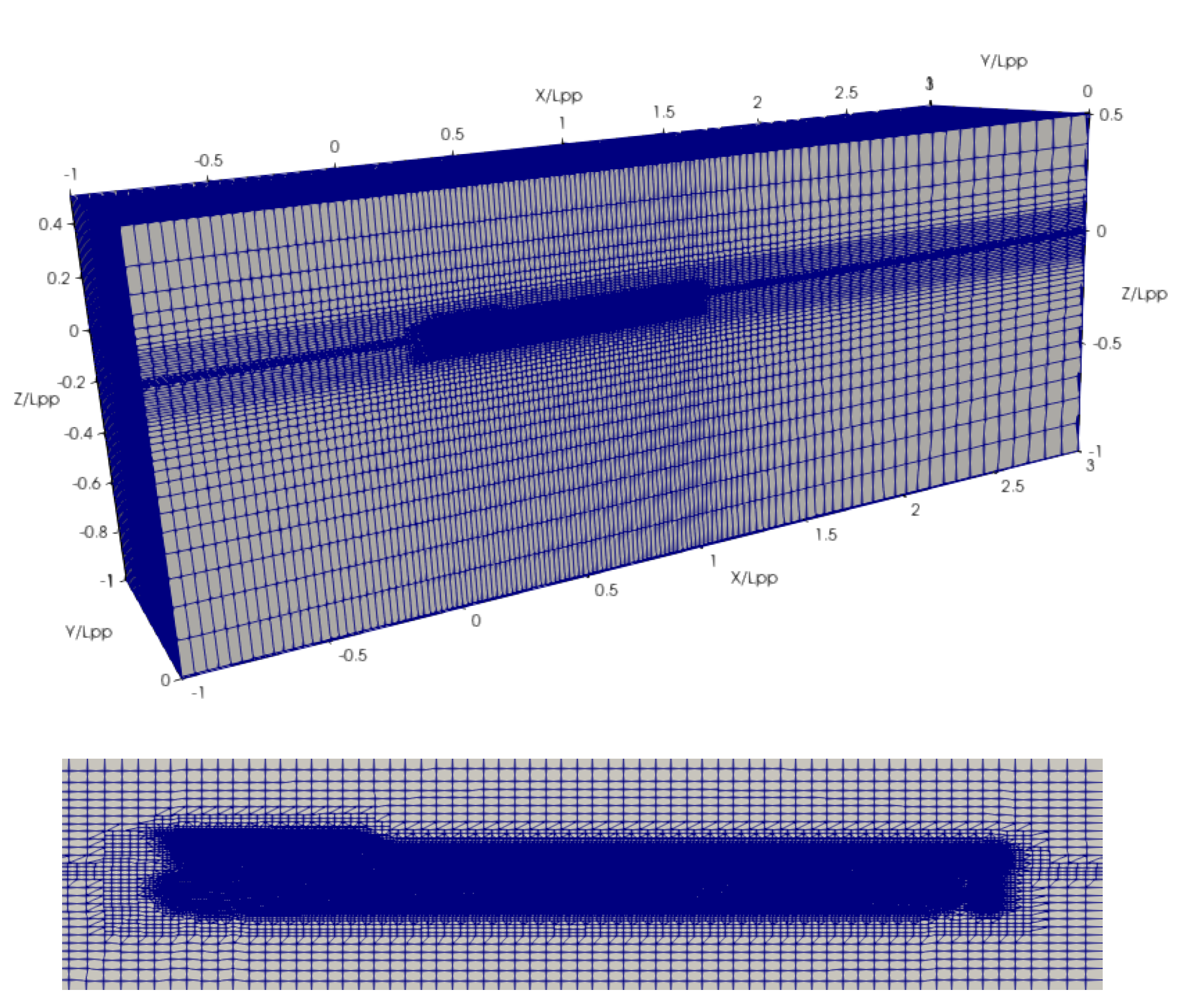
Figure 18 shows the computational domain and the local mesh refinement around the ship. The dimensions of the computational domain are $4L_{\mathrm{pp}}\times L_{\mathrm{pp}}\times 1.5L_{\mathrm{pp}}$. The boundary conditions are summarized in

Table 7. Summary of the boundary conditions for the mesh convergence study.

Boundary Names	$\mathit{\alpha }$	U	${\mathit{p}}_{\mathbf{rgh}}$
Inlet	waveAlpha	waveVelocity	zeroGradient
Outlet	zeroGradient	zeroGradient	fixedValue
Top	inletOutlet	pressureInletOutletVelocity	totalPressure
Centerline	symmetryPlane	symmetryPlane	symmetryPlane
Hull and rudder	zeroGradient	movingWallVelocity	fixedFluxPressure
Boundary Names	$\tilde{\mathbf{\nu }}$	${\mathbf{\nu }}_{\mathbf{t}}$
Inlet	fixedValue 5.871×10${}^{-6}$	fixedValue 1.27×10${}^{-6}$
Outlet	zeroGradient	zeroGradient
Top	zeroGradient	calculated
Centerline	symmetryPlane	symmetryPlane
Hull and rudder	fixedValue 0	nutUSpaldingWallFuntion

, where the bottom and the far field of the domain are both included in the inlet boundary.

The viscous pressure drag coefficient $C_p$, the frictional drag coefficient $C_v$, and the total drag coefficient $C_T$ are defined as:

$$C_p=\frac{F_p}{\frac{1}{2}\rho U^{2}LT}{C}_v=\frac{F_v}{\frac{1}{2}\rho U^{2}LT}{C}_T=\frac{F_T}{\frac{1}{2}\rho U^{2}LT}$$

(19)

where $F_p,F_v$ and $F_T$ are the viscous pressure drag, frictional drag and the total drag on the ship hull and the rudder.

Table 8. Results of the drag coefficients in the mesh convergence study.

Mesh Name	${\mathit{C}}_{\mathit{p}}$	${\mathit{C}}_{\mathit{v}}$	${\mathit{C}}_{\mathit{T}}$	Exp [29]	Error
Coarse	0.00272	0.01682	0.01954	0.0178	$9.8\%$
Medium	0.00237	0.01686	0.01924	0.0178	$8.1\%$
Fine	0.002244	0.01696	0.01921	0.0178	$7.9\%$

shows the mesh convergence results of the drag coefficients on different meshes. The total drag coefficient $C_T$ shows that the numerical solutions converge with satisfying agreement.

Figure 19 shows the profile of the air–water interface on the ship hull extracted with the volume fraction $\alpha =0.5$. It can be seen that the medium and fine meshes agree closely with each other, while the coarse mesh misses the short wave near the bow. In the following sections, the medium mesh is used for all the simulations considering a balance of accuracy and efficiency.

3.3.2. Simulations with the Rudder at Fixed Deflection Angles

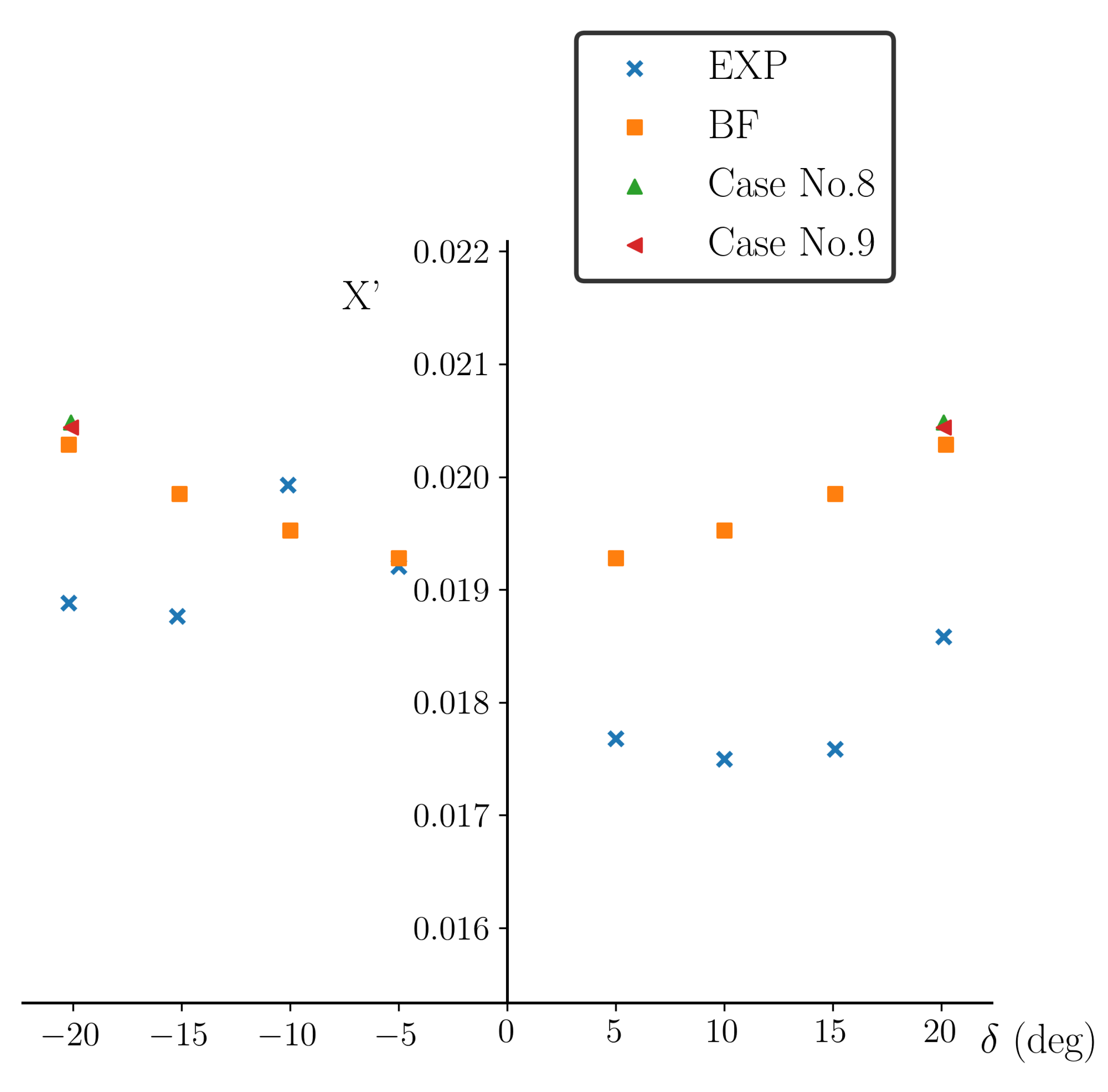
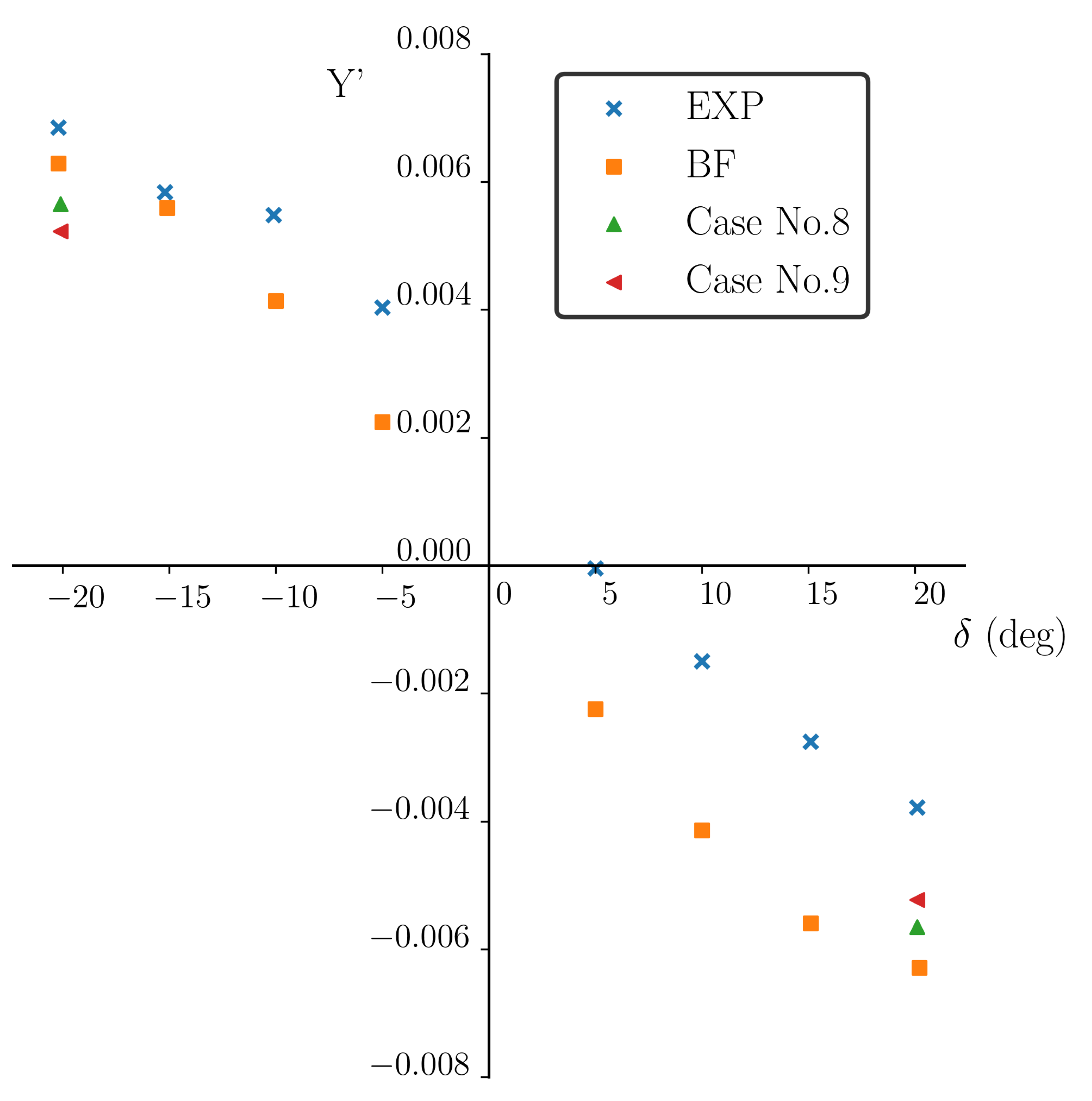
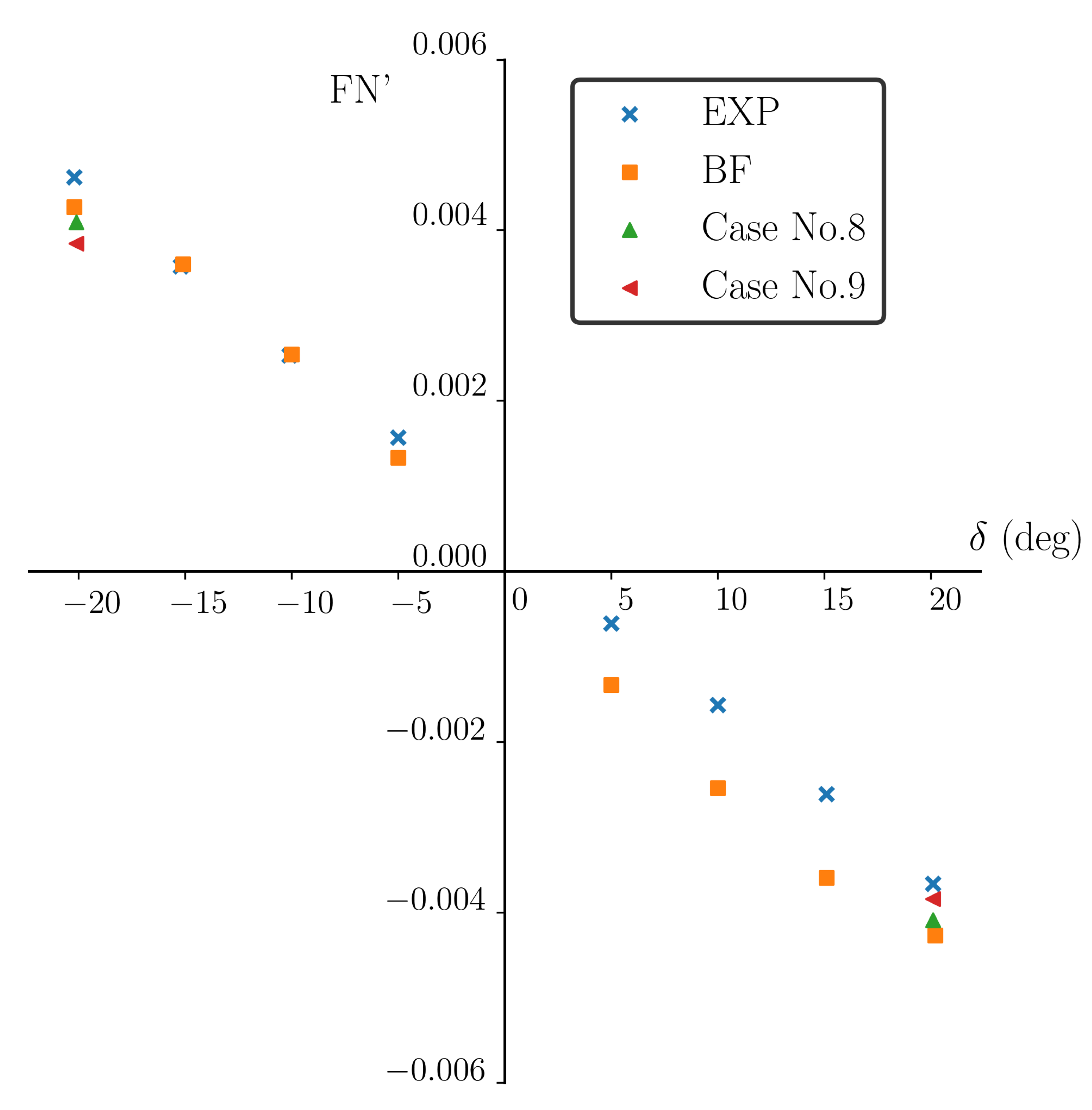
The accuracy of the IBM solver relies on not only the additional operations introduced by the IBM, but also the underlying RANS solver and numerical discretization schemes as discussed in the previous chapters. In this section, the simulations with the rudder at fixed deflection angles using pure body-fitted meshes are carried out. Therefore, the accuracy of the underlying RANS solver and numerical schemes can be evaluated. As a comparison, the case with the rudder at the maximum deflection angle $\delta =-20.1^{\circ }$ is also simulated using the IBM with a fixed IB. Comparisons of the surge coefficient $X^{\prime }$, sway coefficient $Y^{\prime }$ and the normal force coefficient $F{N}^{\prime }$ of the rudder with the experimental data are made to validate the solver. The coefficients are defined in Equation (20) as:

$$X^{\prime }=\frac{X}{\frac{1}{2}\rho U^{2}LT}{Y}^{\prime }=\frac{F_v}{\frac{1}{2}\rho U^{2}LT}F{N}^{\prime }=\frac{FN}{\frac{1}{2}\rho U^{2}LT}$$

(20)

where X and Y are the surge and sway forces on the ship including the rudder, respectively. $FN$ is the force on the moving part of the rudder in the direction normal to the rudder mid plane.

Since the ship hull with the deflected rudder is not symmetric, the medium mesh used in the previous section is mirrored with respect to its centerline. The total number of cells used by both the body-fitted mesh and the IBM is listed in

Table 9. Total number of cells for the simulations of the rudder at fixed deflection angles.

Mesh Name	Body-Fitted	Hybrid
Number of cells	2,441,378	2,499,112

.

Figure 20, Figure 21 and Figure 22 show the results of the force coefficients $X^{\prime }$, $Y^{\prime }$ and $F{N}^{\prime }$, respectively. In the figures, “BF” represents the results of cases No. 4–7 in Table 5. It should be noted that in the experiments tests were carried out at $\delta =\pm 5^{\circ },\pm {10}^{\circ },\pm 15.1^{\circ }$ and $\pm 20.1^{\circ }$. The numerical results generated for positive deflection angles, but are reflected accordingly with respect to the y axis to compare with the full range of experimental data.

Inspection of the experimental data highlights some of the challenges in measuring and predicting rudder forces at model scale. At this model scale Reynolds number, fully turbulent flow may be difficult to maintain along the length of the hull, and the flow patterns in the stern and on the rudder are very sensitive to any asymmetry in the model geometry and setup in the tank. For example, without a propeller, it is expected that a positive and negative rudder angle of the same degree would produce the same drag, whereas this is not exactly the case in the experiments. Likewise, the sway force should pass through zero as the rudder is in its zero position, and again there is a slight positive sway force in the experiments. Figure 20 shows that when $\delta >-{15}^{\circ }$, the total drag is well predicted by OpenFOAM. However, when $\delta \le -{15}^{\circ }$ the numerical results overpredict the drag. It is because when the deflection angle is large, the flow massively separates from the surface of rudder. The Spalart–Allmaras turbulence model used in the current simulation is not fully capable of capturing the massive flow separation on the rudder. In addition, the wall function that is used in the IBM is based on the near-wall velocity profile in an attached turbulent flow, which does not hold true when the deflection angle is large. Compared between the results of Cases No.8 and No.9, it shows that the usage of the wall function does not have notable impact on the total drag. It may because that the rudder is in the region of the wake flow, where the boundary layer effect is not as significant as on the ship hull.

Figure 21 shows that the numerical prediction of the sway force matches well with the experimental data at all deflection angles. The sway force increases consistently with the increase of the deflection angle. It makes sense since the dominant contribution of the sway force comes from the lift force on the rudder, and the lift force increases with the increase of the deflection angle. The prediction of the IBM at the maximum rudder angle is less than the results on the body-fitted mesh, while both results fall into the uncertainty region of the experimental data. In addition, the IB wall function used in the IBM has no notable influence on the sway force.

Figure 22 shows the force on the moving part of the rudder in the direction normal to the rudder mid plane. Again, the numerical predictions match well at all deflection angles. The results at the maximum deflection angle obtained by the body-fitted mesh and the IBM agree well with each other, which again validates the accuracy of the IBM. The result without using the IB wall function underpredicts the normal force on the rudder. In the circumstance of simulating turbulent flows at high Reynolds numbers, it is almost unavoidable for the IBM to have similar near-wall resolution as the body-fitted mesh if the total number of cells is similar. Although due to the fact that the rudder is in the wake flow, the boundary layer effect is not as significant as on the ship hull. Using the IB wall function still improves the overall accuracy, especially when it only slightly increases the computational time.

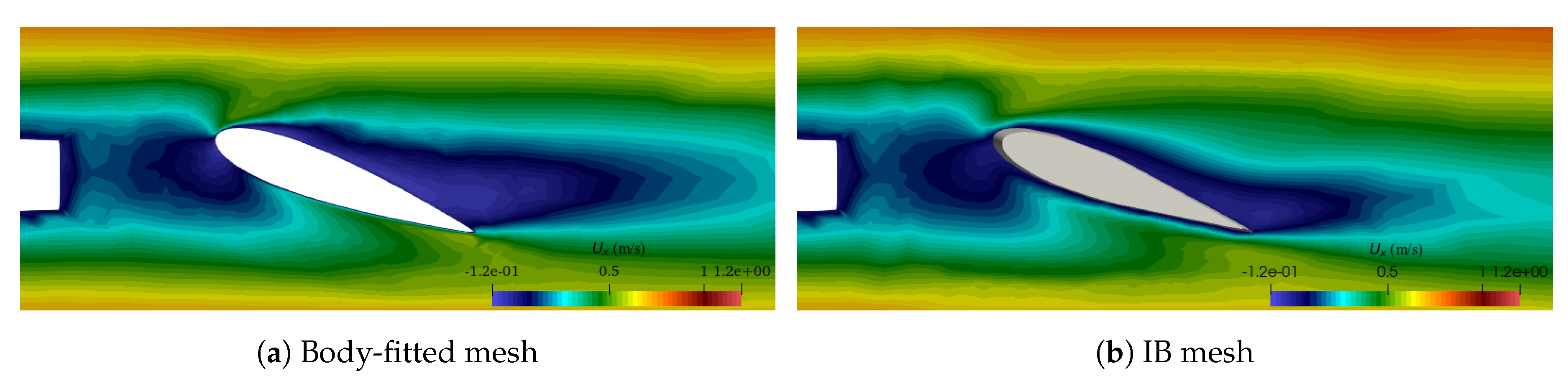
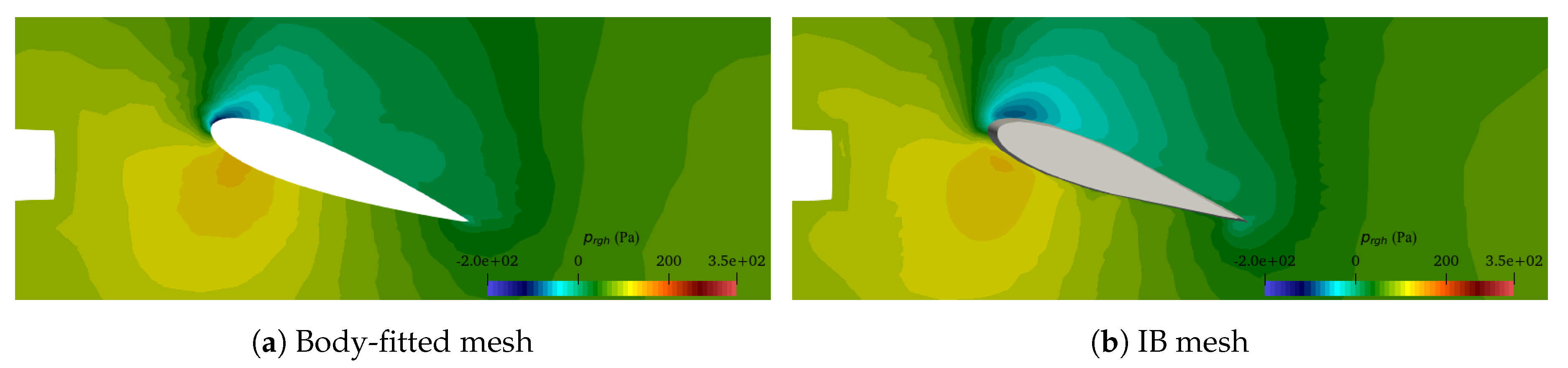
Finally, Figure 23 and Figure 24 show the velocity and dynamic pressure at $z=-0.065\mathrm{m}$ when $\delta =-20.1^{\circ }$, respectively. The velocity field shows the flow separation happens at this deflection angle, which confirms the discussion about the forces on the rudder in the previous paragraphs. For both the velocity and the pressure, the results of the IBM match closely with the body-fitted results.

4. Conclusions

In this paper, we extended our work of single-phase IBM for RANS simulations of fixed and moving objects in air–water two-phase turbulent flows. The VoF method with a compression term was used to simulate the air–water interface. Compared with the simulations of single-phase flows, the momentum equation for two-phase flows has the gradient of density term because of buoyancy. Due to the large ratio of density between air and water, a correct density distribution near the IB surface is necessary to represent the homogeneous Neumann wall condition of density on body-fitted boundaries. This is satisfied indirectly by setting the homogeneous Neumann boundary condition of the volume fraction $\alpha$, and it corresponds to a neutral contact angle boundary condition $\theta =\pi /2$. In the present work, the volume fraction $\alpha$ is extended into the solid domain by a field extension operation. The process involves interpolation of $\alpha$ one layer a time into the solid domain using the inverse square distance method. For turbulence modeling, the same methodology in our previous work is adopted, i.e., the Spalart–Allmaras turbulence model with an IB wall function.

A series of test cases are presented to evaluate the accuracy of the IBM. The cases consider both fixed and moving IB. Various aspects are carefully investigated, including the deformation of the air–water interface, the flow fields and the forces on the IB surfaces. Comparisons between the present results and other resourses demonstrate that the proposed IBM is capable of simulating the interaction between the air–water interface and the solid boundaries. Finally, we investigate the simulation of a KCS ship model advancing with a rotating rudder. The accuracy and flexibility of the IBM is fully demonstrated via the combined usage of the IB surfaces with unstructured body-fitted approach.

References

- Peskin, C.S. Flow patterns around heart valves: A numerical method. J. Comput. Phys. 1972, 10, 252–271. [Google Scholar] [CrossRef]
- Saiki, E.; Biringen, S. Numerical simulation of a cylinder in uniform flow: Application of a virtual boundary method. J. Comput. Phys. 1996, 123, 450–465. [Google Scholar] [CrossRef]
- Beyer, R.P.; LeVeque, R.J. Analysis of a one-dimensional model for the immersed boundary method. SIAM J. Numer. Anal. 1992, 29, 332–364. [Google Scholar] [CrossRef]
- Lai, M.C.; Peskin, C.S. An immersed boundary method with formal second-order accuracy and reduced numerical viscosity. J. Comput. Phys. 2000, 160, 705–719. [Google Scholar] [CrossRef] [Green Version]
- Goldstein, D.; Handler, R.; Sirovich, L. Modeling a no-slip flow boundary with an external force field. J. Comput. Phys. 1993, 105, 354–366. [Google Scholar] [CrossRef] [Green Version]
- Khadra, K.; Angot, P.; Parneix, S.; Caltagirone, J.P. Fictitious domain approach for numerical modelling of Navier–Stokes equations. Int. J. Numer. Methods Fluids 2000, 34, 651–684. [Google Scholar] [CrossRef]
- Mohd-Yusof, J. Combined immersed-boundary/B-spline methods for simulations of ow in complex geometries. Annu. Res. Briefs NASA Ames Res. Cent. Stanf. Univ. Cent. Turbul. Res. Stanf. 1997, 161, 317–327. [Google Scholar]
- Fadlun, E.; Verzicco, R.; Orlandi, P.; Mohd-Yusof, J. Combined immersed-boundary finite-difference methods for three-dimensional complex flow simulations. J. Comput. Phys. 2000, 161, 35–60. [Google Scholar] [CrossRef]
- Balaras, E. Modeling complex boundaries using an external force field on fixed Cartesian grids in large-eddy simulations. Comput. Fluids 2004, 33, 375–404. [Google Scholar] [CrossRef]
- Choi, J.I.; Oberoi, R.C.; Edwards, J.R.; Rosati, J.A. An immersed boundary method for complex incompressible flows. J. Comput. Phys. 2007, 224, 757–784. [Google Scholar] [CrossRef]
- Kalitzin, G.; Iaccarino, G. Turbulence modeling in an immersed-boundary RANS method. Annu. Res. Briefs 2002, 415–426. Available online: https://ctr.stanford.edu/annual-research-briefs-2002 (accessed on 24 September 2020).
- Capizzano, F. Turbulent wall model for immersed boundary methods. AIAA J. 2011, 49, 2367–2381. [Google Scholar] [CrossRef]
- Dommermuth, D.G.; O’Shea, T.T.; Wyatt, D.C.; Ratcliffe, T.; Weymouth, G.D.; Hendrikson, K.L.; Yue, D.K.; Sussman, M.; Adams, P.; Valenciano, M. An application of cartesian-grid and volume-of-fluid methods to numerical ship hydrodynamics. In Proceedings of the 9th International Conference Numerical Ship Hydrodynamics, Ann Arbor, MI, USA, 5–8 August 2007. [Google Scholar]
- Hirt, C.W.; Nichols, B.D. Volume of fluid (VOF) method for the dynamics of free boundaries. J. Comput. Phys. 1981, 39, 201–225. [Google Scholar] [CrossRef]
- Hibiki, T.; Ishii, M. One-dimensional drift-flux model and constitutive equations for relative motion between phases in various two-phase flow regimes. Int. J. Heat Mass Transf. 2003, 46, 4935–4948. [Google Scholar] [CrossRef] [Green Version]
- Sanders, J.; Dolbow, J.E.; Mucha, P.J.; Laursen, T.A. A new method for simulating rigid body motion in incompressible two-phase flow. Int. J. Numer. Methods Fluids 2011, 67, 713–732. [Google Scholar] [CrossRef]
- Shen, L.; Chan, E.S. Numerical simulation of fluid–structure interaction using a combined volume of fluid and immersed boundary method. Ocean Eng. 2008, 35, 939–952. [Google Scholar] [CrossRef]
- Yang, J.; Stern, F. Sharp interface immersed-boundary/level-set method for wave–body interactions. J. Comput. Phys. 2009, 228, 6590–6616. [Google Scholar] [CrossRef]
- Sun, X.; Sakai, M. Numerical simulation of two-phase flows in complex geometries by using the volume-of-fluid/immersed-boundary method. Chem. Eng. Sci. 2016, 139, 221–240. [Google Scholar] [CrossRef]
- Sussman, M. An adaptive mesh algorithm for free surface flows in general geometries. In Adaptive Method of Lines; Chapman and Hall/CRC: Boca Raton, FL, USA, 2001; pp. 227–252. [Google Scholar]
- Calderer, A.; Kang, S.; Sotiropoulos, F. Level set immersed boundary method for coupled simulation of air/water interaction with complex floating structures. J. Comput. Phys. 2014, 277, 201–227. [Google Scholar] [CrossRef] [Green Version]
- Ye, H.; Chen, Y.; Maki, K. A discrete-forcing immersed boundary method for turbulent-flow simulations. Proc. Inst. Mech. Eng. Part M J. Eng. Marit. Environ. 2020. [Google Scholar] [CrossRef]
- Spalart, P.; Allmaras, S. A one-equation turbulence model for aerodynamic flows. In Proceedings of the 30th Aerospace Sciences Meeting and Exhibit, Reno, NV, USA, 6–9 January 1992; p. 439. [Google Scholar]
- Raad, P.E.; Bidoae, R. The three-dimensional Eulerian–Lagrangian marker and micro cell method for the simulation of free surface flows. J. Comput. Phys. 2005, 203, 668–699. [Google Scholar] [CrossRef]
- Lin, S.Y.; Chen, Y.C. A pressure correction-volume of fluid method for simulations of fluid–particle interaction and impact problems. Int. J. Multiph. Flow 2013, 49, 31–48. [Google Scholar] [CrossRef]
- Kleefsman, T. Water impact loading on offshore structures-a numerical study. Ph.D. Thesis, University of Groningen, Groningen, The Netherlands, November 2005. [Google Scholar]
- Miao, G. Hydrodynamic Forces and Dynamic Response of Circular Cylinders in Wave Zones. Ph.D. Thesis, University of Trondheim, Trondheim, Norway, 1989. [Google Scholar]
- Zhu, X.; Faltinsen, O.M.; Hu, C.; Straub, D.; Faber, M.H.; Morris-Thomas, M.T.; Irvin, R.J.; Thiagarajan, K.P.; Storhaug, G.; Moe, E.; et al. Water Entry and Exit of a Horizontal Circular Cylinder. J. Offshore Mech. Arct. Eng. 2007, 129, 253–264. [Google Scholar] [CrossRef]
- Yoshimura, Y.; Fukui, H.Y.; Yano, H. Mathematical Model for Manoeuvring Simulation including Roll motion. Conference Proceedings The Japan Society of Naval Architects and Ocean Engineers. Jpn. Soc. Nav. Archit. Ocean. Eng. 2013, 16, 17–20. [Google Scholar]
Figure 1.
Categories of domains: a. solid domain: white cells; b. forcing domain: red cells; c. fluid domain: blue cells
Figure 2.
Extension of α into the solid region. The IB surfaces are denoted as white dots.
Figure 3.
Comparison of the shape of the water volume. Left: Field extension; middle: no enforcement of the BC; Right: body-fitted mesh.
Figure 4.
Case setup of Dam-Break No.1.
Figure 5.
Relative position between the IB and the medium background mesh.
Figure 6.
Simulation of the 3D dam-break problem with a vertical square obstacle.
Figure 7.
Time history of the horizontal velocity in front of the obstacle at using different background meshes.
Figure 8.
Time history of the impact force on the obstacle using different background meshes.
Figure 9.
Case setup of the 3D dam-break problem with an obstacle: Problem No.2.
Figure 10.
Locations of the pressure sensors P1, P3, P5 and P7.
Figure 11.
Time histories of the water elevation at different locations.
Figure 12.
Time histories of the pressure at different locations.
Figure 13.
Air entrapped on the top of the obstacle in the dam-break problem No.2.
Figure 14.
Computational domain and the initial condition of the water exit of a circular cylinder.
Figure 15.
Time histories of the exit coefficient Ce for the water exit tests.
Figure 16.
Comparison of the profiles of the air–water interface at different time instants in Case No.1. Top row:zhu et al. [28]; bottom row: Present.
Figure 17.
Geometry of the KCS ship model and the rudder.
Figure 18.
Computational domain and the local mesh refinement.
Figure 19.
Free-surface profile on the ship hull with .
Figure 20.
Surge force coefficient predicted at the fixed deflection angles.
Figure 21.
Sway force coefficient predicted at the fixed deflection angles.
Figure 22.
Normal force coefficient of the rudder predicted at the fixed deflection angles.
Figure 23.
Comparison of the velocity at z = −0.065 m when δ = −20.1°.
Figure 24.
Comparison of the dynamic pressure at z = −0.065 m when δ = −20.1°.