Determination of the Grain Size in Single-Phase Materials by Edge Detection and Concatenation

Abstract

This paper presents a novel approach for edge detection and concatenation. It applies the proposed method on a set of optical microscopy images of aluminium alloy Al 99.5% (ENAW1050A) samples with different grain size values. The performance of the proposed approach is evaluated based on the intercept method and compared with the manual grain size determination method. Edge detection filters have proven inefficient in grain boundaries’ detection of the presented microscopy images. To some extent only the Canny edge-detection filter was able to compute grain boundaries of lower-resolution images adequately, while the presented method proved to be superior, especially in high-resolution images. The proposed method has proven its applicability, and it implies higher automatisation and lower processing times compared to manual optical microscopy image processing.

1. Introduction

The task of metallography is to determine and analyse, at a certain chemical composition, the structure and constituting components of metals and alloys. This task is completed by analysing images of the macro- and microstructures. Furthermore, utilising metallography, it is possible to detect defects in the metal material and to find the causes of these defects. In this way, it is possible to determine the most favourable microstructure for a certain production process, which, further, leads to better process control and its improvement and development. By macroscopic examination, the macrostructure is evaluated, and larger defects such as cracks, pores, and similar are detected. Macroscopic techniques are often used for quality control, fracture analysis, and as an introduction to microscopic examinations. A microscopic examination determines the details of the microstructure (phases, boundaries, size, orientation, and shape of the grains), the transformations in solid state, it detects smaller defects (inclusions, inhomogeneities, cracks), and the thickness of layers. Furthermore, it is possible to measure the microhardness of the identified microstructure constituents by additional mechanical testing.

The development of a new microscopy technique enabled the achievement of a high resolution and obtained the image of the microstructure. However, the, interpretation of the obtained results is still a process, where the knowledge of the examiner (scientist, researcher, engineer) determines the performance in interpreting the obtained image and therefore the understanding of material behaviour and properties. This understanding is limited by the education of the examiner, his/her concentration, experience, and knowledge. Consequently, it follows that although the development of microscopic techniques enabled the results to be obtained fast and easily, the interpretation of these results is still highly susceptible to the subjective assessment of the examiner.

In recent years, research in microstructure data science has begun to explore the utilisation of machine vision and image processing. Image processing and analysis can help handle large volumes of image data and facilitate the work of the examiners [1]. The use of filters, which represent projection functions, has been applied to different image processing problems [2,3,4]. Decost et al. [5] applied unsupervised and supervised machine learning techniques to yield insight into microstructural trends and their relationship to processing conditions in ultrahigh carbon steel. Zhang et al. [6] implemented fuzzy logic to extract the grain boundaries of high-strength aluminium alloy microstructure digital images, while Dengiz et al. [7] combined a fuzzy logic algorithm and Neural Network (NN) algorithms for grain boundary detection of super alloy steel optical microstructure images. Gajalakshmi et al. [8] developed an image processing algorithm to determine an average grain size in metallic microstructures by counting the number of grains, with the use of Otsu and Canny edge detection techniques and a support vector regression. Vanderesse et al. [9] employed image processing techniques to distinguish between inter- and intra-granular delta phase precipitates in Inconel 718. Griesser and O’Leary [4] used orientational entropy filtering to determine the orientation of dendrites in metallurgical micrographs of solidified steel. Heilbroner [10] used a gradient-based filtering method named Lazy Grain Boundary (LGB) for grain boundary detection with the stacking of multiple images. Ma et al [11] employed a deep learning-based method for 2D semantic segmentation for grain boundary detection.

However, all the approaches described in the literature mentioned above have some drawbacks: a higher degree of complexity (except when using filters or kernels for instance), the need for training data (in the case of the use of machine learning techniques) and also the end result is never compared directly to a skilled human examiner’s measurements. For that reason, a new grain boundary detection procedure is presented in this paper. The proposed sequence of image processing tasks enables the detection of the grain boundary and edge concatenation by connecting the edges. The developed method is used for grain size measurements and is compared to other conventional and edge retrieval procedures.

2. Materials and Methods

2.1. Sample Preparation

The material for samples was Al 99.5% (ENAW1050A) with the following chemical composition: 0.02% Cu, 0.003% Mn, 0.016% Mg, 0.13% Si, 0.28% Fe, 0.05% Zn, 0.018% Ti, 0.006% Pb, 0.005% Sn and balance Al. All specimens received an equal treatment to achieve identical initial microstructures. This procedure consisted of initial heat treatment (at 600 °C for 16 h, followed by air cooling), uniaxial upsetting (Rastegaev test) to achieve a logarithmic strain of φ = 0.25, and then again heat treatment (at 500 °C for 1 h) to initiate grain growth. In this way, the uniform grain size and chemical homogenisation of specimens were obtained, which was confirmed by microscopic examination and microhardness measurements. The specimens for uniaxial upsetting were cylindrical (Ø 20 × 20 mm) with shallow recesses on the top and bottom surfaces for lubricant application.

For the determination of the relation between the grain size and effective strain value, the specimens were upset uniaxially with logarithmic strain between 0.1 and 1.1. Uniaxial compression achieved a uniform strain distribution through a specimen, and, later, a uniform grain size after recrystallisation. After upsetting, heat treatment (at 500 °C for 1 h) was again required to initiate grain growth. Because specimens were upset for different strain values, each of them had a different grain size. The metallographic observations of grains under polarised light were conducted after the following preparation procedure: grinding with SiC papers (from 220 up to 2500 grid); diamond suspension polishing (6, 3, 1 and 1/4 μm grain size); colloidal silica polishing; the final anodic oxidation etching in Barkers reagent. The detailed procedure of materials upsetting and microstructure examinations was described in reference [12].

2.2. Image Preprocessing Based on the Local Laplacian Pyramid

Pyramid decomposition is a multi-scale signal and image representation method used in the image processing field. A Laplacian pyramid represents a widely used method for image analysis, constructed with spatially invariant Gaussian kernels. The image is broken down into smaller groups of pixels called levels (each level has one-half of the resolution than the previous one, and the original image is situated at level $0$). Each level represents the difference-of-lowpass filters, where the image is decomposed recursively into lowpass and highpass bands. The difference between two adjacent lowpass images of the Gaussian pyramid represents each level in the Laplacian pyramid, where in order to compute the difference, one of the two adjacent lowpass images has to be up-sampled to maintain the appropriate number of dimensions among images. Laplacian pyramids have been believed to be ill-suited for edge-aware operations, resulting in a “halo”-like effect over the edges.

The local Laplacian filters can address these shortcomings. Local Laplacian filters are closely related to bilateral filtering and can be interpreted as a multi-scale version of anisotropic diffusion [13]. Local Laplacian filters produce a variety of different effects using the standard Laplacian pyramids. The discussed method was introduced by Paris et al. [14] in which edges are preserved and the details enhanced simultaneously. The algorithm they used offers a robust method and enables a wide range of effects manipulation. The algorithm’s performance can be altered by setting up the three parameters (${\sigma }_L$, $\alpha$ and $\beta$). Sigma ${\sigma }_L$ defines a difference between small variations (that is considered as a texture) and a larger one (such as an edge), $\alpha$ is a parameter for altering the level of detail, and $\beta$ parameter for dynamic range compression.

2.3. Gaussian Smoothing

Most images are affected by unexplained variation in data or noise. Noise can also be considered as a disturbance in image intensity, which is either not of interest or uninterpretable. The Gaussian filter, besides the moving average, is one of the most widely used smoothing filters. Gaussian filters have weights specified by the probability density function of a normal distribution with variance ${\sigma }_G^2$. The Gaussian filter can also be used to smooth and interpolate between image pixels simultaneously. At location $\left(x,y\right)$, where $y$ is the row index and $x$ the column index, the estimated output intensity is an average of local pixel values, weighted by the Gaussian density function:

$$g\left(x,y\right)= {\displaystyle \sum }_{i=\left|y-3{\sigma }_G\right|}^{i=\left|y+3{\sigma }_G\right|}{\displaystyle \sum }_{j=\left|x-3{\sigma }_G\right|}^{j=\left|x+3{\sigma }_G\right|}\frac{f_{ij}}{2\pi {\sigma }_G^2}\exp \left(\frac{-\left[{\left(i-y\right)}^2+{\left(j-x\right)}^2\right]}{{\sigma }_G^2}\right)$$

(1)

where $f_{ij}$ denote the pixel values in the image.

2.4. Zhang’s Thinning Algorithm

The digitised binary image can, by image processing, be represented as a matrix $IT\left(i,j\right)$, where each point is either $0$ (a white point) or $1$ (a dark point). Following convention, the depicted pattern consists of 1s (dark points). The thinning process transforms the pattern iteratively into a thin line drawing (also known as a skeleton), by deleting the specific dark points. The thinning takes place in a parallel manner, meaning the pixel’s value in the current iteration depends on the value of the pixel and its neighbours at the previous $\left(n-1\right)th$ iteration, so all the picture points can be processed simultaneously.

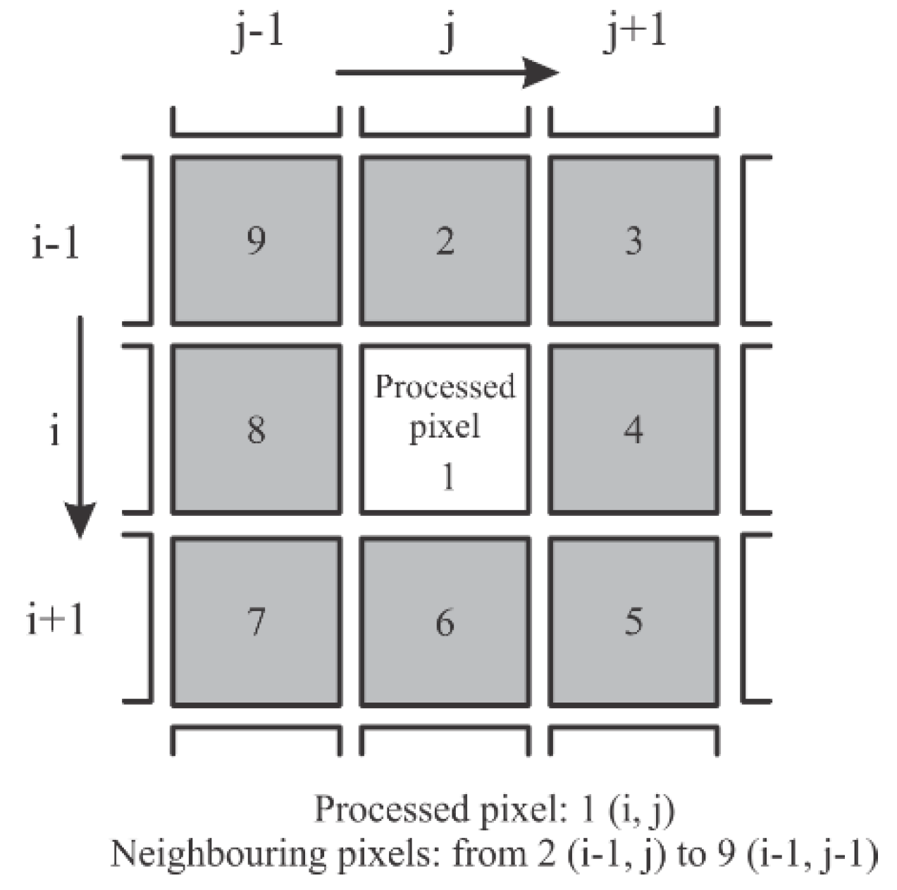
Zhang’s thinning algorithm employs a 3 × 3 kernel, where the point $\left(i,j\right)$ in the middle is connected with its eight neighbouring points $\left(i-1, j\right)$, $\left(i-1,j+1\right)$, $\left(i,j+1\right)$, $\left(i+1,j+1\right)$, $\left(i+1,j\right)$, $\left(i+1,j-1\right)$, $\left(i,j-1\right)$ and $\left(i-1,j-1\right)$ as shown in Figure 1. When using only simple computations, the algorithm removes contour points to extract the skeleton. Each iteration is divided into two subiterations in order to preserve the continuity of the skeleton in congruence with Zhang’s thinning algorithm [15].

2.5. Connecting the Edges Procedure

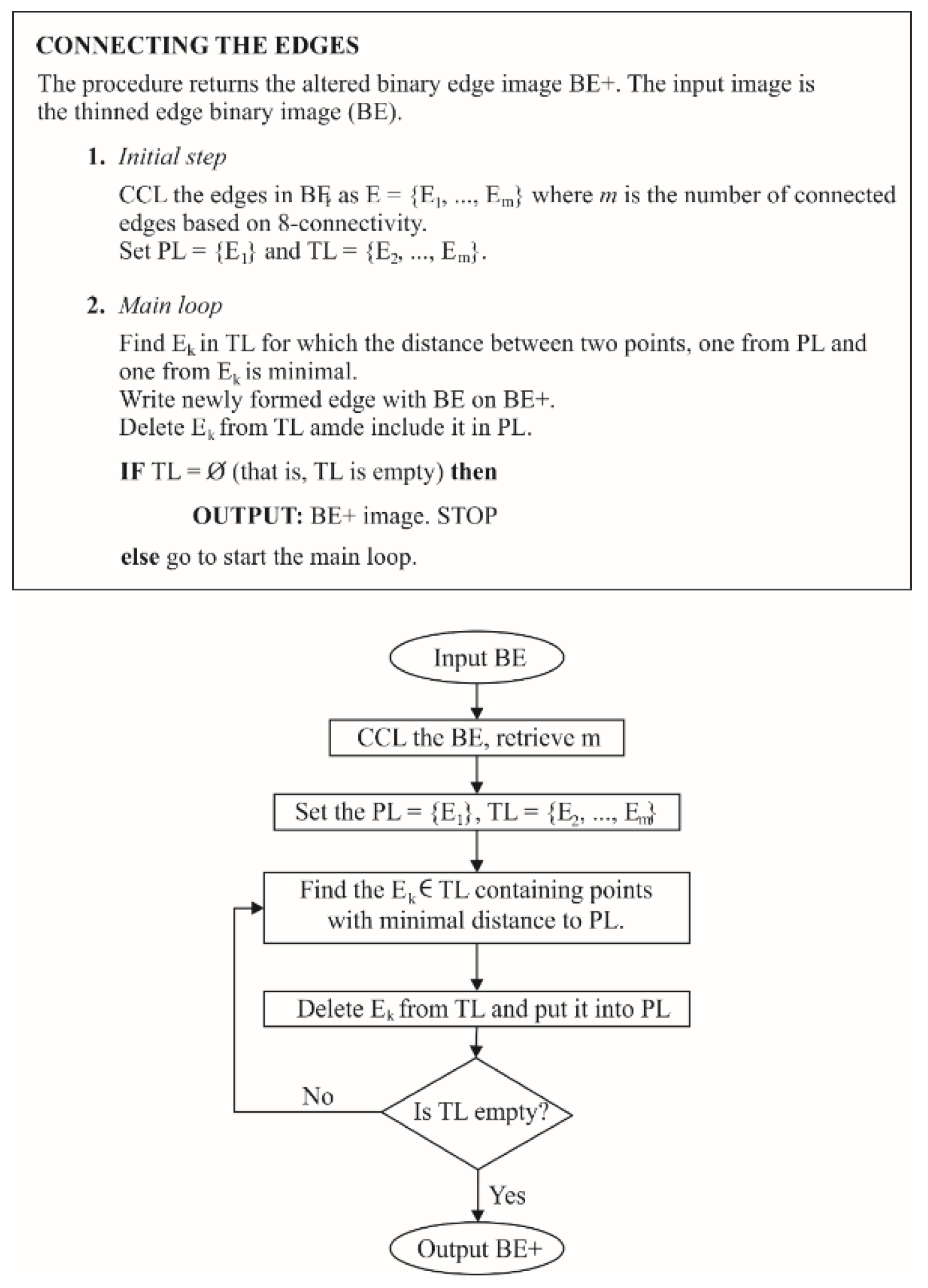
Concatenation is performed by the procedure of connecting the edges and is depicted in Figure 2. In the first step, the binary edges image is processed with the Connected Components Labelling (CCL) method [16] to find and index the continuously connected edges. Connectivity is determined as an 8- or 4-connected neighbourhood. The number of different sets $m$ is computed representing connected edges. The procedure starts with two sets of labels: a permanent label $PL=\left[E_1\right]$ and temporary label $TL=\left[E_2,\dots ,E_m\right]$, where $E_j$ is comprised of two vectors representing $x$ and y coordinates of the connected edge belonging to the $j$-th connected component of binary edge (BE) image. The next step is repeated throughout the procedure the $m-1$ iterations, where $m$ is defined as the number of all connected regions in the BE. In every iteration the two closest points are found, based on the Euclidean distance from sets PL and TL. In the next step, the closest points are connected with a straight line by altering the original binary image. Certain line represents the newly formed edge, previously not detected by edge the retrieval process. Elements and their respective indexes of connected components are grouped, and the newly acquired connected edge, represented as a set of points belonging to $TL$, is removed from the $TL$ set and placed in $PL$. The whole iteration procedure of finding the closest points among sets $PL$ and $TL$ is then repeated until the $TL$ set is empty, or exactly $m-1$ times.

2.6. Grain Size Determination—Conventional Method

A quantitative analysis of the apparent grain size was conducted according to procedure EN ISO 643:2012. To obtain the apparent grain size, a circular intercept method was used, which, according to Standard EN ISO 643:2012, averages out variations in the shape of equiaxed grains and avoids the problem of lines ending within grains. The recognition of grains’ boundaries was performed manually, by an optical (eye) recognition of grain boundaries on the obtained microstructure pictures. The circular intercept method [17] with $3$ concentric circles was used for the measurement.

The obtained mean intersected segment (l) was multiplied by $1.106$ (the average ratio of the mean diameter of the grain and mean intersected segment according to Standard EN ISO 643:2012) to obtain a mean diameter of grains (d). In this way, grain size was determined for each specimen with a uniform strain distribution [12].

2.7. Newly Proposed Method for Grain Size Determination

The aspect of visual perception arises from the human ability to build a conceptual reality; machine vision and image processing are set to mimic the discussed human trade with the use of in-silico models. Computers have become able to perceive the visual world. Image processing methods are being adopted widely for providing imaging-based inspections and measurements. The system with incorporated vision is capable of tackling repetitive tasks at high speeds, as well as offering the automation and improvement of production quality. In this sense, image processing techniques are adopted to enable a semi-automatic recognition of microstructure grain boundaries (via our so-called BE and edge connecting BE+ retrieval procedures) and size measurements (via [18]).

The optical microscopy (by equipment Orthoplan, Leitz, Germany) RGB images used in this study consisted of 724 × 724 and 1536 × 1536 pixels. The procedure consists of two parts: in the first, BE image is retrieved with the implementation of the local Laplacian, Gaussian smoothing, gradient and Zhang’s thinning algorithm. To alter the detection of grain boundaries, a simple edge connecting procedure BE+ is introduced and exploit the unconnected edge regions (retrieved by the BE procedure). However, it must be stressed that the produced algorithm enables the manual adding of edges (preliminarily missed by filters) to possibly increase the accuracy of the second part discussed below. In the second part, grain size measurements are performed with the linear intercept method [18], multiplied by 1.106 (according to Standard EN ISO 643:2012) to obtain the mean diameter of the grains (d_mean). Based on the recommendation of Kurzydolwski [19], four equally spaced directions of 0°, 45°, 90° and 135° were used as shown in Figure 3.

3. Results

The implementation of practical image processing using our newly proposed approach and discussion of implementation details is given in the subsequent text.

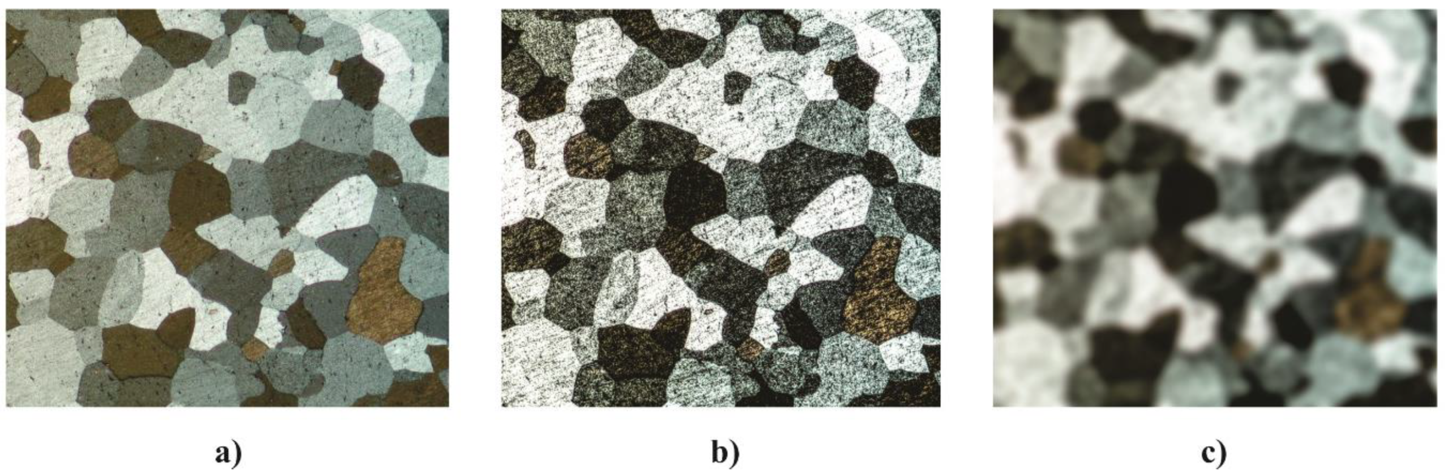
Firstly, the edge retrieval process is explained, which is used to extract the binary image (representing the edges) that serves as a basis for grain size calculations. Figure 4a shows an original (unaltered) specimen’s microstructure image. The Laplacian and Gaussian filters are used for further pre-processing. The local Laplacian filter is an edge-aware processing filter, meaning the large discontinuities (such as edges) remain in place. It is defined with local contrast manipulation parameter $\alpha$, controlling the image detail smoothing, the edge amplitude parameter ${\sigma }_L$ and large-scale variations parameter $\beta$. With the Laplacian filter (Figure 4b), the detail enhancement and the balance is controlled between global and local contrast. The increase in contrast with Laplacian filters enables a better distinction between different grains. After the Laplacian filter use stage, the image is processed further with the use of the Gaussian filter (Figure 4c).

The idea is to use a 2D isotropic Gaussian distribution function, transformed to a discrete kernel form, as a convolution filter for smoothing. The Gaussian filter blurs the processed image to eliminate small image imperfections (such as inclusions or etching artefacts, seen as little black spots on the microstructure image), which have been additionally enhanced with Laplacian, and could disturb the later-on edge extraction. The Gaussian filter also ensures homogeneous colour, along with the specific grain structure. The choice of standard deviation and convolution kernel values (a Gaussian kernel requires $6{\sigma }_G-1$ values to be used for convolution) depends on the application; in this case, the most suitable vales are adopted as given in Figure 4, and further on.

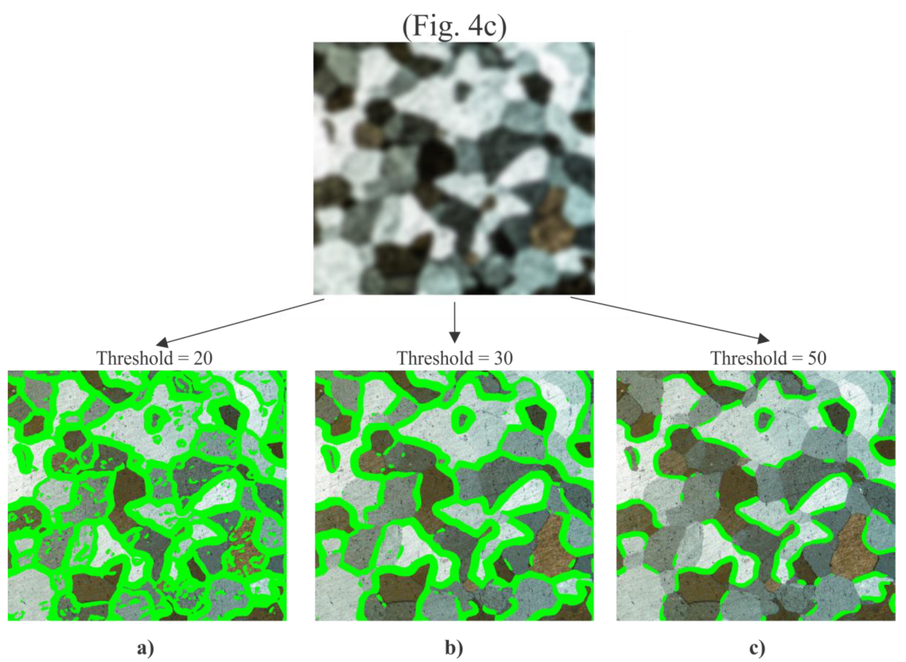
A binary image with enlarged edges was retrieved in the discussed step, wherein a gradient filter based on a Sobel operator with a certain threshold is used on the pre-processed image. The Sobel operator is represented as a 3 × 3 approximation kernel to a derivative of an image. By performing kernel convolution, meaning the gradient matrix is placed over each pixel of an image, we can find out the amount of difference between specific regions in the picture, indicating the presence of an edge. For edge detection, the Sobel-based gradient filter with different threshold values was used, and is depicted in Figure 5. In the case of setting the threshold value too low, too many edges are recognised (Figure 5a), and vice versa for too big threshold values (Figure 5c). The best-suited edge representation is achieved, with a moderate threshold value in case of which only the representative edges are recognised (Figure 5b).

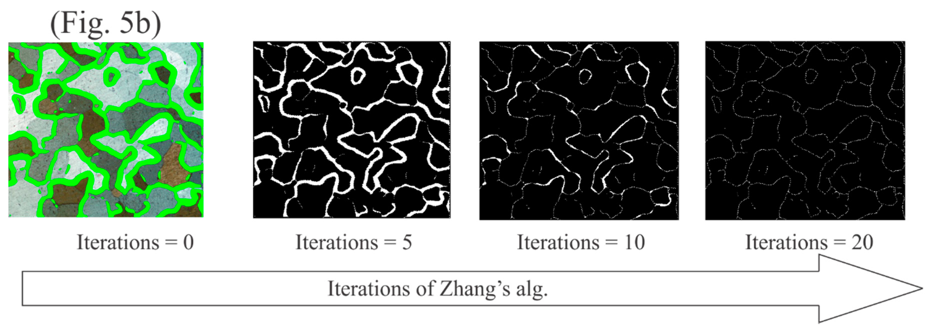
The first part of the proposed method is concluded in the following step, wherein enlarged edges are altered morphologically with the Zhang thinning algorithm. Figure 6 depicts the workings of the thinned edge retrieval procedure, based on the implementation of Zhang’s thinning algorithm after different numbers of iterations. Zhang’s thinning algorithm computed the thinned binary edge (BE) image (BE will also serve as a basis for the BE+ procedure), which can be seen in Figure 6, where edges are only one pixel wide after $20$ iterations. Moreover, the edges can be inserted manually by the examiner (before, or after the thinning phase), to improve the grain size detection rate further.

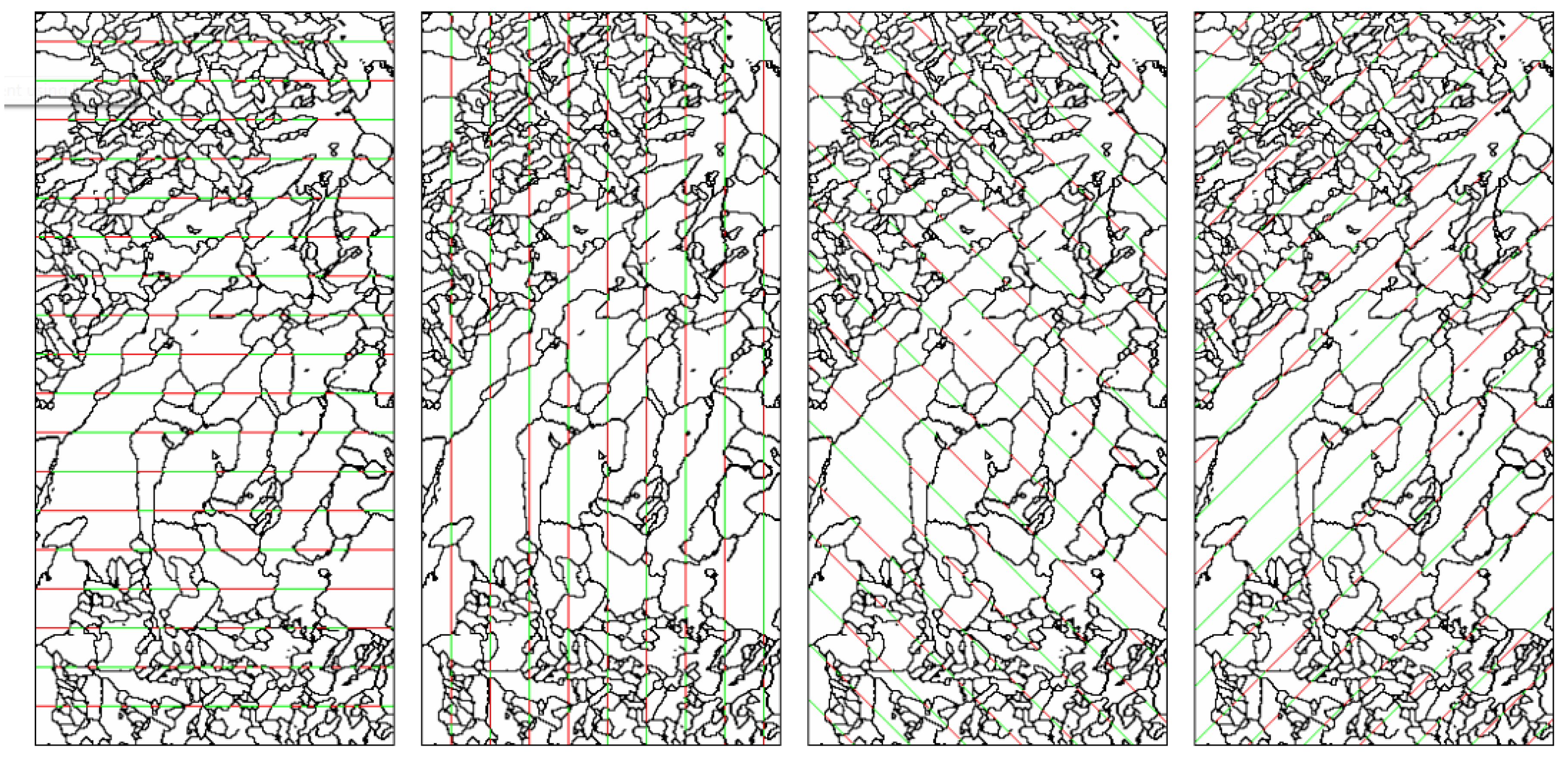
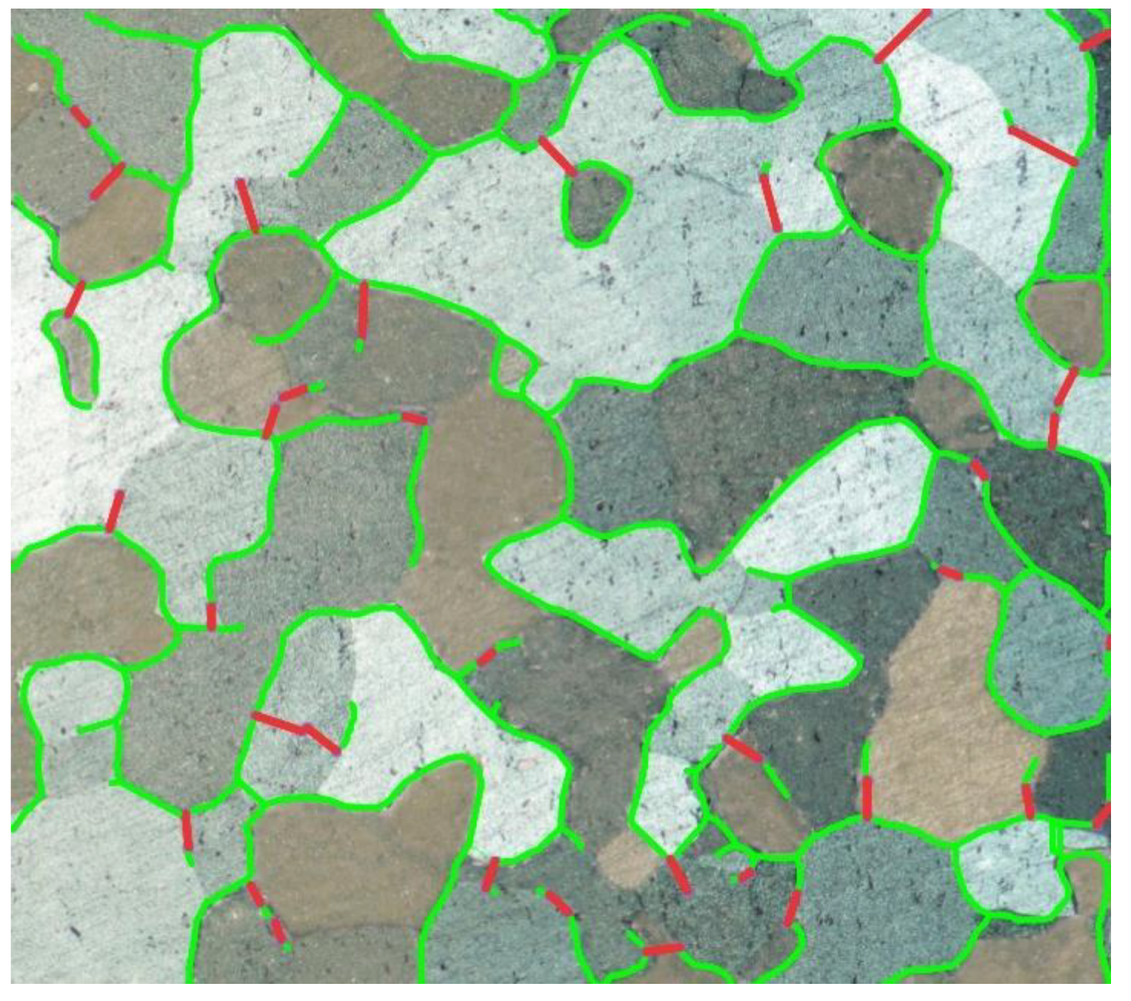
The binary thinned edges image (BE) is processed with the connected components labelling method to find and index the continuously connected edges. Connectivity is determined as an eight-connected neighbourhood. The number of different sets $m$ is computed representing continuously connected edge regions. In every iteration, the two closest points (belonging to different continuously connected edge regions) are found and connected with a straight line, representing the newly formed edge, previously missed by the edge retrieval process (stressing the moderate Sobel filter threshold value is adopted, resulting in multiple unconnected edges as seen in Figure 5b). The so-called connected binary edge image BE+ is computed after all the edge regions are connected into a single region. The workings of the proposed edges connecting procedure BE+ is depicted in Figure 7, where the newly formed edges are shown as red lines, while green regions represent BE.

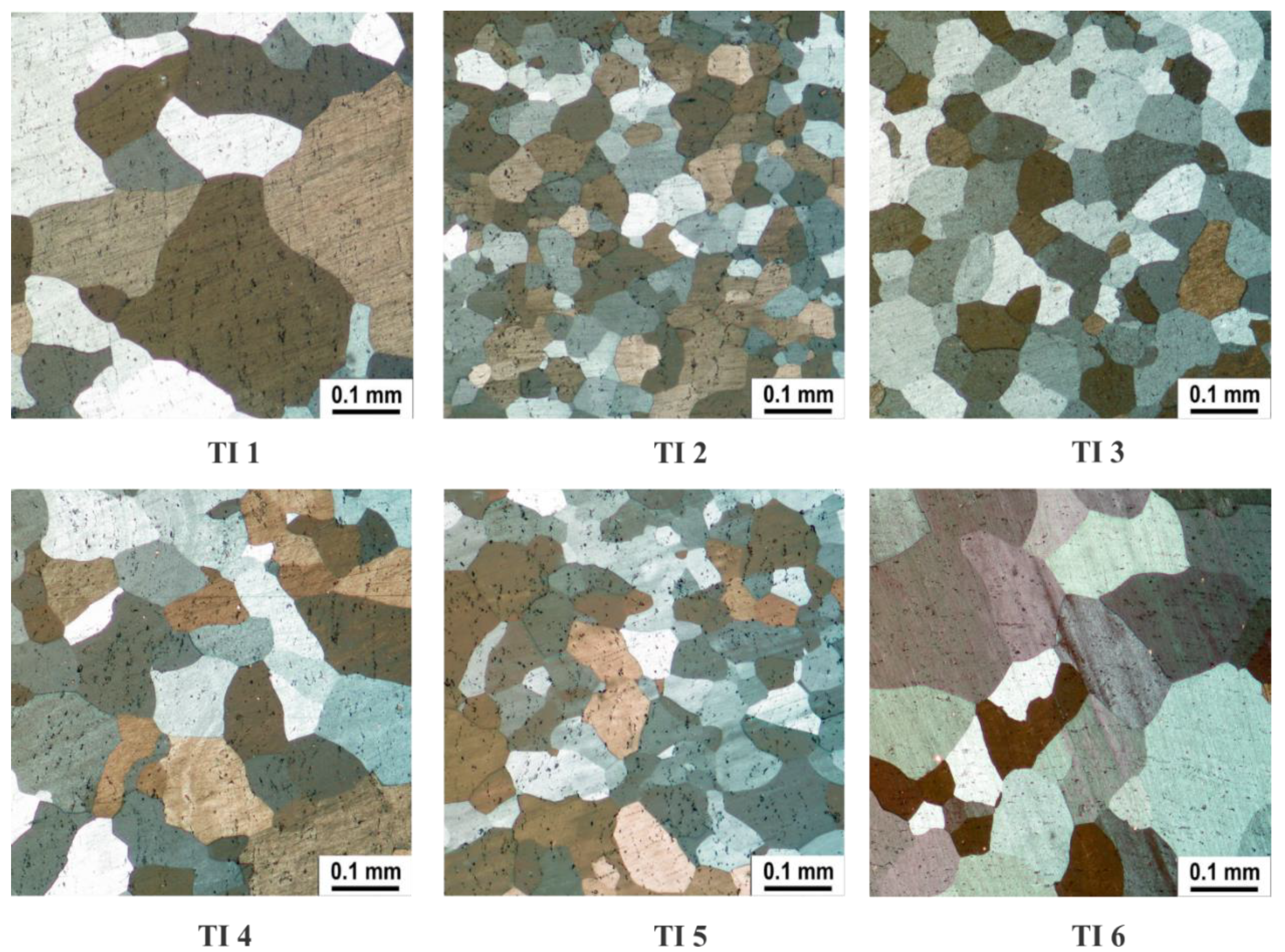
The precision rates of the edge detection procedures presented, BE (without connecting the edges) and BE+ (with connecting the edges procedure), are compared with the conventional method (EN ISO 643:2012) and the Canny-based edge detection procedures. All test images (TIs), depicted in Figure 8, are enhanced with the local Laplace filter with parameters $\alpha =0.1$, ${\sigma }_L=0.5$ and $\beta =0$. The value of the Gaussian blur standard deviation and convolution kernel values (a Gaussian kernel requires $6{\sigma }_G-1$ values to be used for convolution) was set to ${\sigma }_G=8$ for a smaller resolution TI, and ${\sigma }_G=16$ for a larger resolution TI. The threshold of the Sobel gradient filter for the smaller-resolution TI set was equal to $30$ and for the larger-resolution TI was set to $15$. The thinned binary edge image in the case of BE and BE+ was retrieved within $20$ iterations for all TIs.

The basic parameters of the linear intercept method [18] were set as follows. The vertical and horizontal intercept line spacings were set to $10$ pixels, while $45$° and $135$° were set to $14$ pixels since $10/\sin 45°\approx 14$ ensured equal line spacings compared to the horizontal and vertical directions.

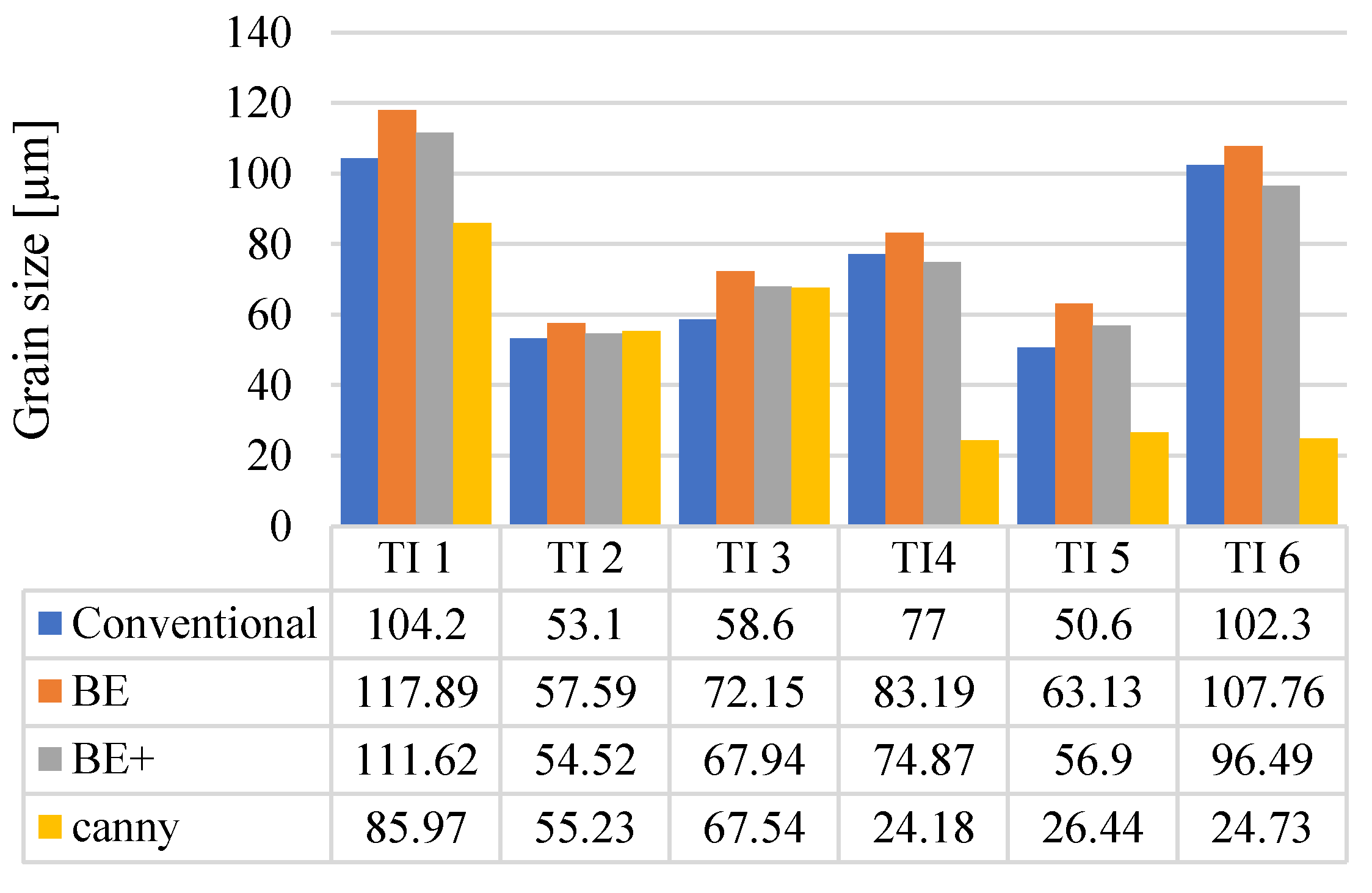
The results of grain size measurements with conventional, Canny, BE and BE+ methods, for all TI are stated in Figure 9. On TI6 the best accuracy achieved with BE, was $5.33$% higher compared to the conventional method (supposing the conventional method achieved 100% accuracy). Meanwhile, TI3 BE achieved the worst accuracy—$24.76$% higher compared to conventional methods. With the BE+ method, the best accuracy of $2.67$% was achieved when processing TI2, while the worst accuracy of $15.94$% was achieved when processing TI3 (compared to the conventional method). Test images with higher resolutions, TI4, TI5 and TI6, achieved lower grain size accuracy rates compared with the lower-resolution test images (TI1, TI2 and TI3) via the Canny edge detection technique [3]. BE and BE+ precision rates indicate the robustness of the proposed method. In concordance with logic, the grain size measurement of BE is always greater compared to BE+, since BE is a subset of BE+ (BE⊆BE+).

Popular edge detection kernels, such as Roberts, Sobel and Prewitt, were not able to recognize the grain boundaries adequately, and were, therefore, omitted from the study. The results for the Canny filter were achieved by setting the threshold ratio to $0.4$, and the high threshold value was defined as 70% of pixels not considered as edges, meaning, among all recognised edges, only 70% of the pixels will be considered as edges. The standard deviation of the Gaussian filter sigma was equal to $\sqrt{2}$ for all TI using the Canny edge detection procedure.

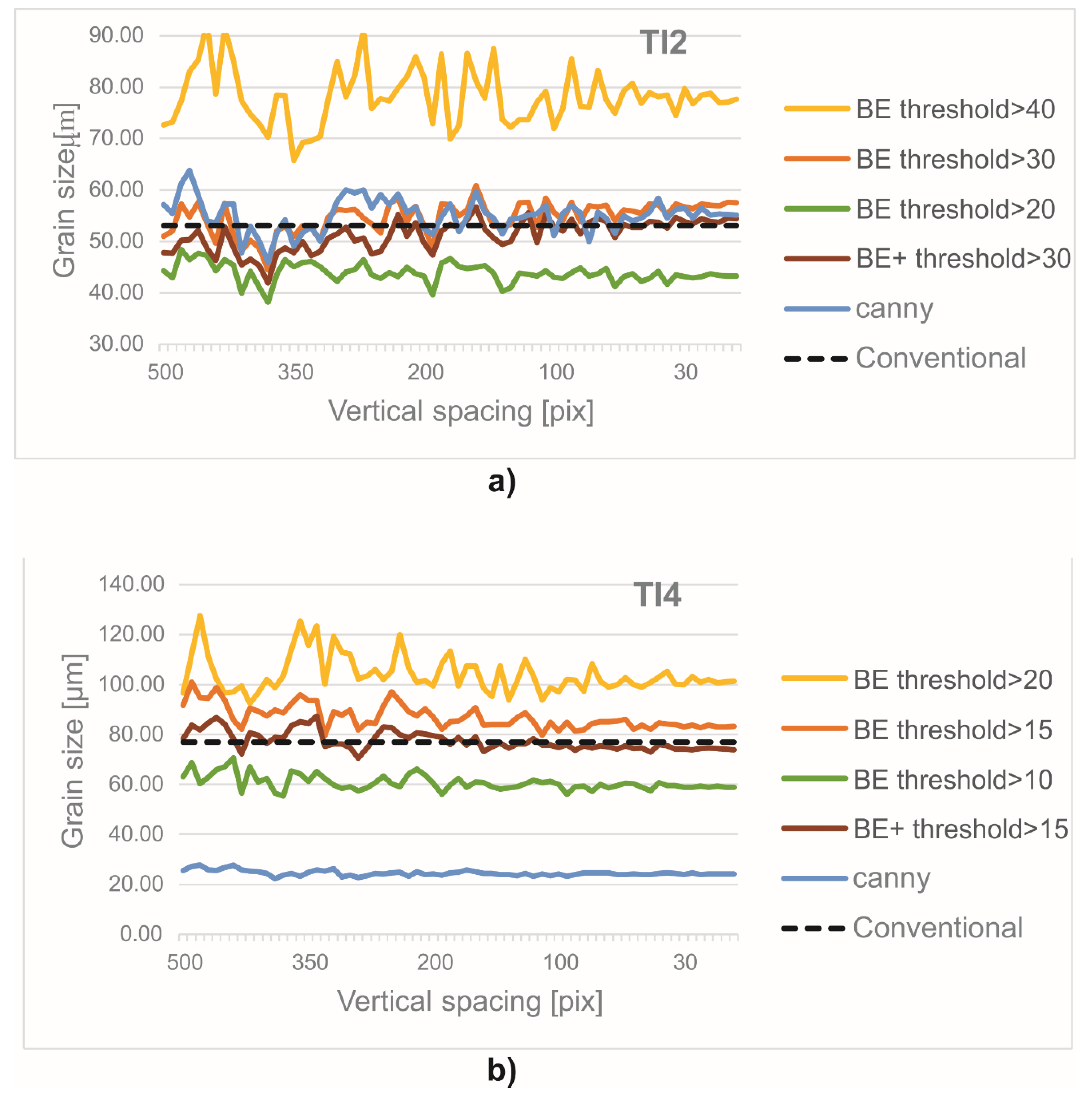
The graphs in Figure 10 display the grain size measurements of the discussed methods on images TI2 (Figure 10a) and TI4 (Figure 10b), and their dependence on the increase in the vertical (equal to horizontal) spacing among intercept lines from 500 to 5 pixels (the $45$° and $135$° directions spacings are equal to vertical spacing/sin45° pixels). Image processing parameters were kept fixed as in the previous processings of TI2 and TI4. The graphs indicate that using $30$ or less pixels for vertical spacing should provide a converged result for grain size measurements, even if the TI4, which has higher resolution, has an earlier and more stable convergence rate. Changing the gradient filter’s threshold value has a noticeable impact on grain size measurements, since lower threshold values give lower grain size measurements and vice versa. This stresses the enduring importance of visual conformation in precise edge detections and grain size measurements with image processing techniques.

4. Discussion

In the presented study, the “specimens” grain size characteristics were detected based on microstructure images and an innovative image processing procedure. The conventional methods of grain size measurements include the use of the planimetric method for image analysis, where the recognition of grains’ boundaries is completed manually, by optical (eye) recognition on obtained microstructure pictures implemented via an examiner. It is established that the discussed procedure is fairly time-consuming and requires a high amount of the examiner’s concentration, as well as high levels of experience and high observatory skills.

The newly suggested image processing workflows (BE and BE+) offer a faster alternative and are for the most part performed automatically. Only a few parameters ought to be set by the examiner. These parameters are the pre-processing settings of local Laplace filter, Gaussian blur, the threshold value for edge detection based on a gradient filter and the number of thinning iterations of Zhang’s algorithm. Additionally, after an automatic edge retrieval procedure, these missed edges can be added manually by the examiner or processed further with connecting the edges procedure to achieve a higher degree of accuracy.

The methods proposed here are compared based on the obtained mean grain size diameter values. The grain diameter values of the proposed methods (BE and BE+) were found to be comparable with those evaluated by the conventional methods and have outperformed the classical edge detection techniques. The BE+ procedure gave the most comparable results to the conventionally (manually) determined grain size results, with negligible disappearances in practical use. It should be stressed that the requirement for BE+ is the existence of the unconnected edges (edge regions). Unconnected edges are, in the case of BE, recovered with moderate gradient filter threshold values.

In future work, it is recommended to build a large dataset of test images and construct a regression machine learning model even further to increase the grain size detection accuracy (without the need of setting the image processing parameters), and shorten the single image processing time. Modified gradient filter kernels and kernel combinations should be implemented and tested since this study only presents the basic edge detection filters. Further application of the proposed edge extraction algorithm in other similar problems is encouraged, to evaluate further the algorithm’s usability. The authors encourage the use of developed methods in macroscopical problems, such as determination of aluminium foam cells size [21] and similar ones in the Image Processing and Measurements domain [22]. The authors also encourage further assessment of BE and BE+ robustness, since these two simple procedures were only tested on 20 sample images overall.

5. Conclusions

This paper presents a novel approach to Optical microscopy grain size determination based on image processing. The paper includes an innovative sequence of image processing tasks (BE and BE+), which enables the edge detection, and edge concatenation by the connecting the edges procedure.

Edge detection filters have proven insufficient in the recognition of the grain boundaries of the presented metallographic images, and were, consequently, incapable of grain size computation. The proposed edge detection protocols BE and BE+ also outperformed the Canny edge detection-based determination of grain sizes when tested on high-resolution images. For the lower-resolution image test sets, the Canny edge filter gave similar results compared to the proposed approach.

Similar grain size recognition rates of the proposed edge detection protocols BE and BE+ to manual grain size determination approaches, performed by a competent and experienced examiner, imply the presented method’s potential and calls for its testing in other fields and applications.

References

- Bulgarevich, D.S.; Tsukamoto, S.; Kasuya, T.; Demura, M.; Watanabe, M. Pattern recognition with machine learning on optical microscopy images of typical metallurgical microstructures. Sci. Rep. 2018, 8, 2078. [Google Scholar] [CrossRef] [PubMed]
- Gorsevski, P.V.; Onasch, C.M.; Farver, J.R.; Ye, X. Detecting grain boundaries in deformed rocks using a cellular automata approach. Comput. Geosci. 2012, 42, 136–142. [Google Scholar] [CrossRef]
- Canny, J. A Computational Approach to Edge Detection. IEEE Trans. Pattern Anal. 1986, 8, 679–698. [Google Scholar] [CrossRef]
- Griesser, S.; O’Leary, P. A new approach for the automatic evaluation of the solidification structure in steel using orientational entropy filtering. J. Microsc.-Oxf. 2014, 253, 161–165. [Google Scholar] [CrossRef] [PubMed]
- DeCost, B.L.; Francis, T.; Holm, E.A. Exploring the microstructure manifold: Image texture representations applied to ultrahigh carbon steel microstructures. Acta Mater. 2017, 133, 30–40. [Google Scholar] [CrossRef] [Green Version]
- Zhang, L.; Xu, Z.; Wei, S.; Ren, X.; Wang, M. Grain Size Automatic Determination for 7050 Al Alloy Based on a Fuzzy Logic Method. Rare Metal Mat. Eng. 2016, 45, 548–554. [Google Scholar] [CrossRef]
- Dengiz, O.; Smith, A.E.; Nettleship, I. Grain boundary detection in microstructure images using computational intelligence. Comput. Ind. 2005, 56, 854–866. [Google Scholar] [CrossRef]
- Gajalakshmi, K.; Palanivel, S.; Nalini, N.J.; Saravanan, S.; Raghukandan, K. Grain size measurement in optical microstructure using support vector regression. Optik 2017, 138, 320–327. [Google Scholar] [CrossRef]
- Vanderesse, N.; Anderson, M.; Bridier, F.; Bocher, P. Inter- and intragranular delta phase quantitative characterization in Inconel 718 by means of image analysis. J. Microsc.-Oxf. 2015, 261, 79–87. [Google Scholar] [CrossRef] [PubMed]
- Heilbronner, R. Automatic grain boundary detection and grain size analysis using polarization micrographs or orientation images. J. Struct. Geol. 2000, 22, 969–981. [Google Scholar] [CrossRef]
- Ma, B.; Liu, C.; Wei, X.; Gao, M.; Ban, X.; Wang, H.; Huang, H.; Xue, W. WPU-Net: Boundary learning by using weighted propagation in convolution network. arXiv 2019, arXiv:1905.09226. [Google Scholar]
- Skakun, P.; Rajnovic, D.; Janjatovic, P.; Balos, S.; Shishkin, A.; Novak, P.; Sidjanin, L. Metallographic Determination of Strain Distribution in Cold Extruded Aluminum Gear-Like Element. Metals 2020, 10, 589. [Google Scholar] [CrossRef]
- Aubry, M.; Paris, S.; Hasinoff, S.W.; Kautz, J.; Durand, F. Fast Local Laplacian Filters: Theory and Applications. ACM Trans. Graph. 2014, 33, 167. [Google Scholar] [CrossRef] [Green Version]
- Paris, S.; Hasinoff, S.; Kautz, J. Local Laplacian Filters: Edge-aware Image Processing with a Laplacian Pyramid. ACM Trans. Graph. 2011, 30, 68. [Google Scholar] [CrossRef]
- Zhang, T.Y.; Suen, C.Y. A fast parallel algorithm for thinning digital patterns. Commun. ACM 1984, 27, 236–239. [Google Scholar] [CrossRef]
- Haralick, R.M.; Shapiro, L.G. Computer and Robot Vision (Volume 2); Addison-Wesley: Boston, MA, USA, 1993; pp. 28–48. [Google Scholar]
- Abrams, H. Grains size Measurement by the Intercept Method. Metallography 1971, 4, 59–78. [Google Scholar] [CrossRef]
- Lehto, P.; Remes, H.; Saukkonen, T.; Hänninen, H.; Romanoff, J. Influence of grain size distribution on the Hall–Petch relationship of welded structural steel. Mater. Sci. Eng. A 2014, 592, 28–39. [Google Scholar] [CrossRef] [Green Version]
- Kurzydłowski, K.J. A model for the flow stress dependence on the distribution of grain size in polycrystals. Scr. Metall. Mater. 1990, 24, 879–883. [Google Scholar] [CrossRef]
- Aalto University Wiki, Characterization of Average Grain Size and Grain Distribution. Available online: https://wiki.aalto.fi/display/GSMUM/Characterization+of+average+grain+size+and+grain+size+distribution (accessed on 5 October 2020).
- Razborsek, B.; Gotlih, J.; Karner, T.; Ficko, M. The influence of Machining Parameters on the Surface Porosity of a Closed-Cell Aluminium Foam. Stroj. Vestn.-J. Mech. E 2020, 66, 29–37. [Google Scholar] [CrossRef]
- Zuperl, U.; Radic, A.; Cus, F.; Irgolic, T. Visual measurement of layer thickness in multi-layered funcionally graded metal materials. Adv. Prod. Eng. Manag. 2016, 11, 105–114. [Google Scholar] [CrossRef] [Green Version]
Figure 1.
Designations of the nine pixels in a 3 × 3 kernel [15].
Figure 2.
Pseudocode and flowchart of the connecting the edges procedure.
Figure 3.
Measurement of average grain size in a material using the ASTM E1382 linear intercept method [20]. Reproduced with permission from Pauli Lehto, Aalto University Wiki; published by Aalto University.
Figure 4.
The original microstructure image (a) contrast manipulation (b) with an enhancement of the picture details, while preserving edges based on a local Laplacian filter with , and . Gaussian filtering (c) to blur the image with 2D 47 × 47 convolution kernel and standard deviation .
Figure 5.
Sobel gradient filter different threshold values (a), (b) in (c).
Figure 6.
Zhang’s thinning algorithm used to compute binary edge images.
Figure 7.
Procedure for connection of the edges procedure; green regions represents binary edge (BE), image combined green and red regions represent BE+.
Figure 8.
Tested images TI1, TI2, TI3, TI4, TI5 and TI6. Image sizes vary from 724 × 724 (for TI1, TI2 and TI3) to 1536 × 1536 (for TI4, TI5 and TI6).
Figure 9.
Results of average grain size predictions of tested images TI1 to TI6, based on the conventional method, BE, BE+ and Canny edge detection filter.
Figure 10.
BE, BE+ and Canny edge detection grain size measurements with different spacing values for TI2 (a) and TI4 (b), compared to the conventional grain size determination method.
Publisher’s Note: MDPI stays neutral with regard to jurisdictional claims in published maps and institutional affiliations. |
© 2020 by the authors. Licensee MDPI, Basel, Switzerland. This article is an open access article distributed under the terms and conditions of the Creative Commons Attribution (CC BY) license (http://creativecommons.org/licenses/by/4.0/).
Share and Cite
MDPI and ACS Style
Berus, L.; Skakun, P.; Rajnovic, D.; Janjatovic, P.; Sidjanin, L.; Ficko, M. Determination of the Grain Size in Single-Phase Materials by Edge Detection and Concatenation. Metals 2020, 10, 1381. https://doi.org/10.3390/met10101381
AMA Style
Berus L, Skakun P, Rajnovic D, Janjatovic P, Sidjanin L, Ficko M. Determination of the Grain Size in Single-Phase Materials by Edge Detection and Concatenation. Metals. 2020; 10(10):1381. https://doi.org/10.3390/met10101381
Chicago/Turabian StyleBerus, Lucijano, Plavka Skakun, Dragan Rajnovic, Petar Janjatovic, Leposava Sidjanin, and Mirko Ficko. 2020. "Determination of the Grain Size in Single-Phase Materials by Edge Detection and Concatenation" Metals 10, no. 10: 1381. https://doi.org/10.3390/met10101381
Note that from the first issue of 2016, this journal uses article numbers instead of page numbers. See further details here.