Inertial Neural Networks with Unpredictable Oscillations

Abstract

In this paper, inertial neural networks are under investigation, that is, the second order differential equations. The recently introduced new type of motions, unpredictable oscillations, are considered for the models. The motions continue a line of periodic and almost periodic oscillations. The research is of very strong importance for neuroscience, since the existence of unpredictable solutions proves Poincaré chaos. Sufficient conditions have been determined for the existence, uniqueness, and exponential stability of unpredictable solutions. The results can significantly extend the role of oscillations for artificial neural networks exploitation, since they provide strong new theoretical and practical opportunities for implementation of methods of chaos extension, synchronization, stabilization, and control of periodic motions in various types of neural networks. Numerical simulations are presented to demonstrate the validity of the theoretical results.

1. Introduction

In recent decades, dynamicists have focused on the study of neural networks. Many results on stability, periodicity, synchronization analysis, and chaos in neural networks have been published. Some authors investigated neural networks by adding inertia. For example, inertial bidirectional associative memory (BAM) neural networks [1,2,3,4,5,6], inertial Cohen–Grossberg-type neural networks [7,8], electronic neural networks with inertia [9], and inertial memristive neural networks [10,11,12] have been studied.

Oscillations are in a focus of neuroscience, since they correlate with many cognitive tasks. For example, oscillatory neural networks are productive for investigation of image recognition [13,14], as well as activating network states associated with memory recall [15]. They became the core of interdisciplinary research which unites psychophysics, neuroscience, cognitive psychology, biophysics, and computational modeling [16,17]. Chaoticity in neural networks analysis is reflected by data related to experiments and observations [18,19,20].

Artificial neural networks are involved in computing systems and are designed to simulate the way the human brain analyzes and processes information. They are in the foundation of artificial intelligence and solves problems that would prove impossible or difficult by human or statistical standards. Artificial neural networks allow modeling of nonlinear processes, and they have turned into a very popular and useful tool for solving many problems such as classification, clustering, regression, pattern recognition, structured prediction, machine translation, anomaly detection, decision-making, and visualization [21,22,23,24,25,26].

In the present research, a new type of oscillation, which is described by the unpredictable functions, and was introduced in [27], is investigated. The line of periodic and almost periodic motions of neural networks is continued. The Poincaré chaos has already been approved by the existence of unpredictable solutions for a Hopfield type neural network [28] and shunting inhibitory cellular neural networks [29]. The notion of the unpredictable function is strictly connected to the concept of the unpredictable point [27,30,31]. This has been confirmed in papers by Miller [32], Thakur, and Dus [33] in which unpredictable points are very useful for analysis of Poincaré, strongly Ruelle–Takens and strongly Auslander–Yorke chaos in topological spaces. The unpredictable functions are introduced for the analysis of chaos through methods of differential and discrete equations [34,35]. The study of these functions indicates theoretical advantages and problems that apply to both oscillation theory and chaos theory, and this opens up many interesting perspectives in neuroscience.

Our main purpose is to give the conditions ensuring the existence, uniqueness, and asymptotic stability of the unpredictable oscillations in inertial neural networks.

2. Preliminaries

Throughout the paper, $\mathbb{R}$ and $\mathbb{N}$ will stand for the set of real and natural numbers, respectively. Additionally, the norm ${\displaystyle {\parallel v\parallel }_1=\underset{t\in \mathbb{R}}{sup}\parallel v\left(t\right)\parallel ,}$ where ${\displaystyle ∥v∥=\underset{1\le i\le p}{max}\left|v_i\right|,}$$v=(v_1,\dots ,v_p),t,v_i\in \mathbb{R},i=1,...,p,$$p\in \mathbb{N},$ will be used. The following definition is the main one in our study.

Definition 1

([27]). A uniformly continuous and bounded function $v:\mathbb{R}\to {\mathbb{R}}^p$ is unpredictable if there exist positive numbers ${ϵ}_0,\delta$ and sequences $t_n,u_n$ both of which diverge to infinity such that $v(t+t_n)\to v\left(t\right)$ as $n\to \infty$ uniformly on compact subsets of $\mathbb{R}$ and $\parallel v(t+t_n)-v\left(t\right)\parallel \ge {ϵ}_0$ for each $t\in [u_n-\delta ,u_n+\delta ]$ and $n\in \mathbb{N}$.

The convergence of the sequence $v(t+t_n)$ is said to be Poisson stability of the unpredictable function or simply Poisson stability as well as existence of the numbers ${ϵ}_0,\delta$ and the sequence $u_n$ allow the unpredictability property of the unpredictable function.

In this paper, we consider the following inertial neural networks:

$${\displaystyle \frac{d^2{x}_i\left(t\right)}{d{t}^2}=-a_i\frac{d{x}_i\left(t\right)}{dt}-b_i{x}_i\left(t\right)+\sum _{j=1}^p{c}_{ij}{f}_j\left(x_j\left(t\right)\right)+v_i\left(t\right),}$$

(1)

where $t,x_i\in \mathbb{R},i=1,\dots p,p$ denotes the number of neurons in the network, $x_i\left(t\right)$ with $i=1,\dots p,$ corresponds to the state of the unit i at time $t,$ $b_i>0,a_i>0$ are constants, $f_i$ with $i=1,\dots p,$ denote the measures of activation to its incoming potentials of the unit i at time t, $c_{ij}$ for all $i,j=1,\dots p,$ are constants, which denote the connection strength between ith neuron and jth neuron, $v_i\left(t\right)$ are external inputs on the ith neuron at the time $t.$ We assume that the coefficients $c_{ij}$ are real, the activations $f_i:\mathbb{R}\to \mathbb{R}$ are continuous functions that satisfy the following condition:

(C1) 

$|f_i\left(x_1\right)-f_i\left(x_2\right) |\le L_i|x_1-x_2|$ for all $x_1,x_2\in \mathbb{R},$ where $L_i>0$ are Lipschitz constants, for $i=1,\dots ,p,$ and ${\displaystyle \underset{1\le i\le p}{max}{L}_i=L.}$

By introducing the following variable transformation

$$\begin{array}{c}\hfill y_i\left(t\right)={\xi }_i\frac{d{x}_i\left(t\right)}{dt}+{\zeta }_i{x}_i\left(t\right),i=1,\cdots ,p,\end{array}$$

(2)

the neural network (1) can be written as

$$\begin{array}{c}\hfill \left\{\begin{array}{cc}{\displaystyle \frac{d{x}_i\left(t\right)}{dt}=-\frac{{\zeta }_i}{{\xi }_i}{x}_i\left(t\right)+\frac{1}{{\xi }_i}{y}_i\left(t\right),}\hfill & i=1,\cdots ,p,\hfill \\ {\displaystyle \frac{d{y}_i\left(t\right)}{dt}=-(a_i-\frac{{\zeta }_i}{{\xi }_i})y_i\left(t\right)-({\xi }_i{b}_i-{\zeta }_i(a_i-\frac{{\zeta }_i}{{\xi }_i}))x_i\left(t\right)+{\xi }_i\sum _{j=1}^p{c}_{ij}{f}_j\left(x_j\left(t\right)\right)+{\xi }_i{v}_i\left(t\right),}\hfill & i=1,\cdots ,p.\hfill \end{array}\right.\end{array}$$

(3)

According to the results in [36], the couple $x\left(t\right)=(x_1\left(t\right),x_2\left(t\right),\cdots ,x_p\left(t\right)),$$y\left(t\right)=(y_1\left(t\right),y_2\left(t\right),\cdots ,y_p\left(t\right))$ is a bounded solution of (3), if and only if the next integral equations are satisfied:

$$\begin{array}{c}\hfill \left\{\begin{array}{c}{\displaystyle x_i\left(t\right)=\frac{1}{{\xi }_i}{\int }_{-\infty }^t{e}^{-\frac{{\zeta }_i}{{\xi }_i}(t-s)}{y}_i\left(s\right)ds,}\hfill \\ {\displaystyle y_i\left(t\right)={\int }_{-\infty }^t{e}^{-(a_i-\frac{{\zeta }_i}{{\xi }_i})(t-s)}[({\zeta }_i(a_i-\frac{{\zeta }_i}{{\xi }_i})-{\xi }_i{b}_i)x_i\left(s\right)+{\xi }_i\sum _{j=1}^p{c}_{ij}{f}_j\left(x_j\left(s\right)\right)+{\xi }_i{v}_i\left(s\right)]ds,}\hfill \end{array}\right.\end{array}$$

(4)

where $i=1,\cdots ,p.$

The following conditions will be needed throughout the paper:

(C2) 

the functions $v_i\left(t\right),i=1,\cdots ,p,$ in system (1) are unpredictable; they belong to $\Sigma$ and there exist positive numbers $\delta ,{ϵ}_0>0$ and the sequence $s_n\to \infty$ as $n\to \infty ,$ such that $|v_i(t+t_n)-v_i\left(t\right)|\ge {ϵ}_0$ for all $t\in [s_n-\delta ,s_n+\delta ],$$i=1,\dots ,p,$ and $n\in \mathbb{N};$

(C3) 

there exists a positive number $M_f$ such that $\left|f_i\left(s\right)\right|\le M_f,$$i=1,2,\dots ,p,$$\left|s\right|<H.$

There exist positive real numbers ${\xi }_i,{\zeta }_i,$ such that the following inequalities are valid:

(C4) 

${\displaystyle a_i>\frac{{\zeta }_i}{{\xi }_i}+{\xi }_i,\hspace{1em} }$${\zeta }_i>{\xi }_i>1,i=1,\dots ,p;$

(C5) 

${\displaystyle (a_i-\frac{{\zeta }_i}{{\xi }_i})-\left(\right|{\zeta }_i(a_i-\frac{{\zeta }_i}{{\xi }_i})-{\xi }_i{b}_i|+{\xi }_i)>0,}$ for each $i=1,\dots ,p$;

(C6) 

$\frac{{\displaystyle {\xi }_i{M}_f\sum _{j=1}^p{c}_{ij}}}{{\displaystyle (a_i-\frac{{\zeta }_i}{{\xi }_i})-\left(\right|{\zeta }_i(a_i-\frac{{\zeta }_i}{{\xi }_i})-{\xi }_i{b}_i|+{\xi }_i)}}<H,$H is a positive number, $i=1,\dots ,p$;

(C7) 

${\displaystyle \frac{1}{(a_i-\frac{{\zeta }_i}{{\xi }_i})}\left[|{\zeta }_i(a_i-\frac{{\zeta }_i}{{\xi }_i})-{\xi }_i{b}_i|+L{\xi }_i\sum _{j=1}^p{c}_{ij}\right]<1,i=1,\dots ,p;}$

(C8) 

${\displaystyle \underset{i}{max}\left(\frac{1}{{\xi }_i},|{\zeta }_i(a_i-\frac{{\zeta }_i}{{\xi }_i})-{\xi }_i{b}_i|+L{\xi }_i\sum _{j=1}^p{c}_{ij}\right)<\underset{i}{min}\left(\frac{{\zeta }_i}{{\xi }_i},a_i-\frac{{\zeta }_i}{{\xi }_i}\right),i=1,\dots ,p.}$

3. Main Results

In this section, we will use the norm ${\parallel ·\parallel }_1$ for dimensions p and $2p.$ Denote by $\Sigma$ the set of vector-functions, $\phi \left(t\right)=({\phi }_1,\cdots ,{\phi }_{2p})$, such that:

(K1) 

functions $\phi \left(t\right)$ are uniformly continuous;

(K2) 

there exists a positive number H such that ${\parallel \phi \parallel }_1<H$ for all $\phi \left(t\right);$

(K3) 

there exists a sequence, $t_n\to \infty$ as $n\to \infty$ such that $\phi (t+t_n)$ uniformly converges to $\phi \left(t\right)$ on each bounded interval of the real line.

Define on $\Sigma$ an operator $\Pi ,$ such that $\Pi \varphi \left(t\right)=({\Pi }_1{\varphi }_1\left(t\right),{\Pi }_2{\varphi }_2\left(t\right),\cdots ,{\Pi }_{2p}{\varphi }_{2p}\left(t\right)),$ where

$$\begin{array}{ccc}& & {\Pi }_i{\varphi }_i\left(t\right)=\left\{\begin{array}{cc}{\displaystyle \frac{1}{{\xi }_i}{\int }_{-\infty }^t{e}^{-\frac{{\zeta }_i}{{\xi }_i}(t-s)}{\varphi }_{i+p}\left(s\right)ds,}\hfill & i=1,\cdots ,p,\hfill \\ {\displaystyle {\int }_{-\infty }^t{e}^{-(a_{i-p}-\frac{{\zeta }_{i-p}}{{\xi }_{i-p}})(t-s)}[({\zeta }_{i-p}(a_{i-p}-\frac{{\zeta }_{i-p}}{{\xi }_{i-p}})-{\xi }_{i-p}{b}_{i-p}){\varphi }_{i-p}\left(s\right)}\hfill \\ {\displaystyle +{\xi }_{i-p}\sum _{j=1}^p{c}_{(i-p)j}{f}_j\left({\varphi }_j\left(s\right)\right)+{\xi }_{i-p}{v}_{i-p}\left(s\right)]ds,}\hfill & i=p+1,\cdots ,2p.\hfill \end{array}\right.\hfill \end{array}$$

(5)

Lemma 1.

The operator Π is invariant in $\Sigma .$

Proof. 

For a function $\varphi \left(t\right)\in \Sigma$ and fixed $i=1,2,\cdots ,p,$ we have that

$$\begin{array}{ccc}& & |{\Pi }_i{\varphi }_i\left(t\right)|=\left\{\begin{array}{c}{\displaystyle \left|\frac{1}{{\xi }_i}{\int }_{-\infty }^t{e}^{-\frac{{\zeta }_i}{{\xi }_i}(t-s)}{\varphi }_{i+p}\left(s\right)ds\right|\le \frac{1}{{\zeta }_i}\left|{\varphi }_{i+p}\left(t\right)\right|\le \frac{H}{{\zeta }_i},}\hfill \\ i=1,\dots ,p,\hfill \\ {\displaystyle \left|{\int }_{-\infty }^t{e}^{-(a_{i-p}-\frac{{\zeta }_{i-p}}{{\xi }_{i-p}})(t-s)}\right[({\zeta }_{i-p}(a_{i-p}-\frac{{\zeta }_{i-p}}{{\xi }_{i-p}})-{\xi }_{i-p}{b}_{i-p}){\varphi }_{i-p}\left(s\right)}\hfill \\ {\displaystyle +{\xi }_{i-p}\sum _{j=1}^p{c}_{(i-p)j}{f}_j\left({\varphi }_j\left(s\right)\right)+{\xi }_{i-p}{v}_{i-p}\left(s\right)\left]ds\right|}\hfill \\ {\displaystyle \le {\int }_{-\infty }^t{e}^{-(a_{i-p}-\frac{{\zeta }_{i-p}}{{\xi }_{i-p}})(t-s)}\left[|{\zeta }_{i-p}(a_{i-p}-\frac{{\zeta }_{i-p}}{{\xi }_{i-p}})-{\xi }_{i-p}{b}_{i-p}|H+{\xi }_{i-p}\sum _{j=1}^p{c}_{(i-p)j}{M}_f+{\xi }_{i-p}H\right]ds}\hfill \\ {\displaystyle \le \frac{1}{a_{i-p}-\frac{{\zeta }_{i-p}}{{\xi }_{i-p}}}\left[H\left(\right|{\zeta }_{i-p}(a_{i-p}-\frac{{\zeta }_{i-p}}{{\xi }_{i-p}})-{\xi }_{i-p}{b}_{i-p}|+{\xi }_{i-p})+{\xi }_{i-p}{M}_f\sum _{j=1}^p{c}_{(i-p)j}\right],}\hfill \\ i=p+1,\cdots ,2p.\hfill \end{array}\right.\end{array}$$

Conditions (C5), (C6) imply that $|{\Pi }_i{\varphi }_i\left(t\right)|<H,$ for each $i=1,\dots ,2p$—thus that ${∥\Pi \varphi ∥}_1=\underset{i}{max}\left|{\Pi }_i{\varphi }_i\right|<H.$ Thus, condition (K2) is valid.

Let us fix a positive number $ϵ$ and a section $[a,b],-\infty <a<b<\infty .$ We will show that, for sufficiently large n, it is true that $\parallel \Pi \varphi (t+t_n)-\Pi \varphi \left(t\right){\parallel }_1<ϵ$ on $[a,b].$ One can find that

$$\begin{array}{c}|{\Pi }_i{\varphi }_i(t+t_n)-{\Pi }_i{\varphi }_i\left(t\right)=\left\{\begin{array}{c}{\displaystyle \left|\frac{1}{{\xi }_i}{\int }_{-\infty }^t{e}^{-\frac{{\zeta }_i}{{\xi }_i}(t-s)}({\varphi }_{i+p}(s+t_n)-{\varphi }_{i+p}\left(s\right))ds\right|,}\hfill \\ i=1,\dots ,p,\hfill \\ {\displaystyle \left|{\int }_{-\infty }^t{e}^{-(a_{i-p}-\frac{{\xi }_{i-p}}{{\zeta }_{i-p}})(t-s)}\right[({\zeta }_{i-p}(a_{i-p}-\frac{{\zeta }_{i-p}}{{\xi }_{i-p}})-{\xi }_{i-p}{b}_{i-p})({\varphi }_{i-p}(s+t_n)-{\varphi }_{i-p}\left(s\right))}\hfill \\ {\displaystyle +{\xi }_{i-p}\sum _{j=1}^p{c}_{(i-p)j}(f_j({\varphi }_j(s+t_n)-f_j\left({\varphi }_j\left(s\right)\right))+{\xi }_{i-p}(v_{i-p}(s+t_n)-v_{i-p}\left(s\right))\left]ds\right|,}\hfill \\ i=p+1,\dots ,2p.\hfill \end{array}\right.\end{array}$$

Choose numbers $c<a$ and $\xi >0,$ satisfying the following inequalities:

$${\displaystyle \frac{2H}{{\zeta }_i}{e}^{-\frac{{\zeta }_i}{{\xi }_i}(a-c)}<\frac{ϵ}{2},}$$

(6)

$${\displaystyle \frac{2H}{a_i-\frac{{\zeta }_i}{{\xi }_i}}\left(|{\zeta }_i(a_i-\frac{{\zeta }_i}{{\xi }_i})-{\xi }_i{b}_i|+L{\xi }_i\sum _{j=1}^p{c}_{ij}+{\xi }_i\right)e^{-(a_i-\frac{{\zeta }_i}{{\xi }_i})(a-c)}<\frac{ϵ}{2},}$$

(7)

$${\displaystyle \frac{\xi }{{\zeta }_i}<\frac{ϵ}{2}}$$

(8)

$${\displaystyle \frac{\xi }{a_i-\frac{{\zeta }_i}{{\xi }_i}}\left(|{\zeta }_i(a_i-\frac{{\zeta }_i}{{\xi }_i})-{\xi }_i{b}_i|+L{\xi }_i\sum _{j=1}^p{c}_{ij}+{\xi }_i\right)<\frac{ϵ}{2}.}$$

(9)

Consider the number n sufficiently large such that $|{\varphi }_i(t+t_n)-{\varphi }_i\left(t\right)|<\xi ,i=1,\dots ,2p,$ and $|v_i(t+t_n)-v_i\left(t\right)|<\xi ,$ $i=1,\dots ,p,$ on $[c,b]$. Then, for all $t\in [a,b],$ it is true that

$$\begin{array}{c}{\displaystyle |{\Pi }_i{\varphi }_i(t+t_n)-{\Pi }_i{\varphi }_i\left(t\right)|\le \left\{\begin{array}{c}{\displaystyle \left|\frac{1}{{\xi }_i}{\int }_{-\infty }^c{e}^{-\frac{{\zeta }_i}{{\xi }_i}(t-s)}({\varphi }_{i+p}(s+t_n)-{\varphi }_{i+p}\left(s\right))ds\right|}\hfill \\ {\displaystyle +\left|\frac{1}{{\xi }_i}{\int }_c^t{e}^{-\frac{{\zeta }_i}{{\xi }_i}(t-s)}({\varphi }_{i+p}(s+t_n)-{\varphi }_{i+p}\left(s\right))ds\right|\le \frac{2H}{{\zeta }_i}{e}^{-\frac{{\zeta }_i}{{\xi }_i}(a-c)}+\frac{1}{{\zeta }_i}\xi ,}\hfill \\ i=1,\dots ,p,\hfill \\ {\displaystyle \left|{\int }_{-\infty }^c{e}^{-(a_{i-p}-\frac{{\zeta }_{i-p}}{\xi i-p})(t-s)}\right[({\zeta }_{i-p}(a_{i-p}-\frac{{\zeta }_{i-p}}{{\xi }_{i-p}})-{\xi }_{i-p}{b}_{i-p})({\varphi }_{i-p}(s+t_n)-{\varphi }_{i-p}\left(s\right))}\hfill \\ {\displaystyle +{\xi }_{i-p}\sum _{j=1}^p{c}_{(i-p)j}(f_j\left({\varphi }_j(s+t_n)\right)-f_j\left({\varphi }_j\left(s\right)\right))+{\xi }_{i-p}(v_{i-p}(s+t_n)-v_{i-p}\left(s\right))\left]d\tau ds\right|}\hfill \\ {\displaystyle +|{\int }_c^t{e}^{-(a_{i-p}-\frac{{\zeta }_{i-p}}{{\xi }_{i-p}})(t-s)}[({\zeta }_{i-p}(a_{i-p}-\frac{{\zeta }_{i-p}}{{\xi }_{i-p}})-{\xi }_{i-p}{b}_{i-p})({\varphi }_{i-p}(s+t_n)-{\varphi }_{i-p}\left(s\right))}\hfill \\ {\displaystyle +{\xi }_{i-p}\sum _{j=1}^p{c}_{(i-p)j}(f_j\left({\varphi }_j(s+t_n)\right)-f_j\left({\varphi }_j\left(s\right)\right))+{\xi }_{i-p}(v_{i-p}(s+t_n)-v_{i-p}\left(s\right))\left]ds\right|}\hfill \\ {\displaystyle \le \frac{1}{a_{i-p}-\frac{{\zeta }_{i-p}}{{\xi }_{i-p}}}(2H|{\zeta }_{i-p}(a_{i-p}-\frac{{\zeta }_{i-p}}{{\xi }_{i-p}})-{\xi }_{i-p}{b}_{i-p}|}\hfill \\ {\displaystyle +2LH{\xi }_{i-p}\sum _{j=1}^p{c}_{(i-p)j}+2H{\xi }_{i-p})e^{-(a_{i-p}-\frac{{\zeta }_{i-p}}{{\xi }_{i-p}})(a-c)}}\hfill \\ {\displaystyle +\frac{1}{a_{i-p}-\frac{{\zeta }_{i-p}}{{\xi }_{i-p}}}\left(|{\zeta }_{i-p}(a_{i-p}-\frac{{\zeta }_{i-p}}{{\xi }_{i-p}})-{\xi }_{i-p}{b}_{i-p}|\xi +L{\xi }_{i-p}\sum _{j=1}^p{c}_{(i-p)j}\xi +\xi {\xi }_{i-p}\right),}\hfill \\ i=p+1,\dots ,2p.\hfill \end{array}\right.}\end{array}$$

(10)

Now, inequalities (6)–(9) imply that $\parallel \Pi \varphi (t+t_n)-\Pi \varphi \left(t\right){\parallel }_1<ϵ,$ for $t\in [a,b].$ Since $ϵ$ is an arbitrarily small number, condition (K3) is satisfied. Condition (K1) follows from the boundedness of its derivative. The lemma is proved. □

Lemma 2.

The operator Π is a contraction mapping on Σ.

Proof. 

For any $u,v\in \Sigma ,$ one can attain that

$$\begin{array}{c}|{\Pi }_i{u}_i\left(t\right)-{\Pi }_i{v}_i\left(t\right)|=\left\{\begin{array}{cc}{\displaystyle \left|\frac{1}{{\xi }_i}{\int }_{-\infty }^t{e}^{-\frac{{\zeta }_i}{{\xi }_i}(t-s)}(u_{i+p}\left(s\right)-v_{i+p}\left(s\right))ds\right|\le \frac{1}{{\zeta }_i}{\parallel u\left(t\right)-v\left(t\right)\parallel }_1,}\hfill & i=1,\dots ,p,\hfill \\ {\displaystyle \left|{\int }_{-\infty }^t{e}^{-(a_{i-p}-\frac{{\zeta }_{i-p}}{{\xi }_{i-p}})(t-s)}\right[({\zeta }_{i-p}(a_{i-p}-\frac{{\zeta }_{i-p}}{{\xi }_{i-p}})-{\xi }_{i-p}{b}_{i-p})(u_{i-p}\left(s\right)-v_{i-p}\left(s\right))}\hfill \\ {\displaystyle +{\xi }_{i-p}\sum _{j=1}^p{c}_{(i-p)j}(f_{j-p}(u_{j-p}\left(s\right)-f_{j-p}\left(v_{j-p}\left(s\right)\right))\left]ds\right|}\hfill \\ {\displaystyle \le \frac{1}{(a_{i-p}-\frac{{\zeta }_{i-p}}{{\xi }_{i-p}})}[|{\zeta }_{i-p}(a_{i-p}-\frac{{\zeta }_{i-p}}{{\xi }_{i-p}})-{\xi }_{i-p}{b}_{i-p}|}\hfill \\ {\displaystyle +L{\xi }_{i-p}\sum _{j=1}^p{c}_{(i-p)j}]{\parallel u\left(t\right)-v\left(t\right)\parallel }_1,}\hfill & i=p+1,\dots ,2p.\hfill \end{array}\right.\end{array}$$

The last inequality yields ${\displaystyle {\parallel \Pi u-\Pi v\parallel }_1=\underset{i}{max}\left(\frac{1}{{\xi }_i},\frac{1}{(a_i-\frac{{\zeta }_i}{{\xi }_i})}\left[|{\zeta }_i(a_i-\frac{{\zeta }_i}{{\xi }_i})-{\xi }_i{b}_i|+L{\xi }_i\sum _{j=1}^p{c}_{ij}\right]\right){\parallel u-v\parallel }_1.}$ Hence, in accordance with conditions (C4),(C7), the operator $\Pi$ is contractive. □

Theorem 1.

Assume that conditions (C1)–(C8) are fulfilled. Then, the system (1) admits a unique asymptotically stable unpredictable solution.

Proof. 

Let us check the completeness of the space $\Sigma$. Consider a Cauchy sequence ${\varphi }_k\left(t\right)$ in $\Sigma$, which converges to a limit function $\varphi \left(t\right)$ on $\mathbb{R}$. Since conditions (K1) and (K2) are easy to verify, it suffices to show that $\varphi \left(t\right)$ satisfies condition (K3). Fix a closed and bounded interval $I\subset \mathbb{R}.$ We obtain that

$$\begin{array}{ccc}\hfill & & \parallel \varphi (t+t_n)-\varphi \left(t\right)\parallel \le \parallel \varphi (t+t_n)-{\varphi }_k(t+t_n)\parallel +\parallel {\varphi }_k(t+t_n)-{\varphi }_k\left(t\right)\parallel +\parallel {\varphi }_k\left(t\right)-\varphi \left(t\right)\parallel .\hfill \end{array}$$

(11)

If n and k are sufficiently large, then each term on the right-hand side of (11) is smaller than $\frac{ϵ}{3}$ for an arbitrary $ϵ$ and $t\in I$. This means that $\varphi (t+t_n)$ uniformly converges to $\varphi \left(t\right)$ on $I.$ The completeness of space $\Sigma$ is verified. From Lemmas 1, 2 and contraction mapping theorem, it follows that there exists a unique solution $\omega \left(t\right)\in \Sigma$ of Equation (1).

Next, we prove the unpredictability property. It is true that

$$\begin{array}{c}{\omega }_i(t+t_n)-{\omega }_i\left(t\right)=\left\{\begin{array}{c}{\displaystyle {\omega }_i(s_n+t_n)-{\omega }_i\left(s_n\right)-{\int }_{s_n}^t\frac{{\zeta }_i}{{\xi }_i}({\omega }_i(s+t_n)-{\omega }_i\left(s\right))ds}\hfill \\ {\displaystyle +{\int }_{s_n}^t\frac{1}{{\xi }_i}({\omega }_{i+p}(s+t_n)-{\omega }_{i+p}\left(s\right))ds,}\hfill \\ {\displaystyle i=1,...,p,}\hfill \\ {\displaystyle {\omega }_i(s_n+t_n)-{\omega }_i\left(s_n\right)-{\int }_{s_n}^t(a_{i-p}-\frac{{\zeta }_{i-p}}{{\xi }_{i-p}})({\omega }_i(s+t_n)-{\omega }_i\left(s\right))ds}\hfill \\ {\displaystyle -{\int }_{s_n}^t({\zeta }_{i-p}(a_{i-p}-\frac{{\zeta }_{i-p}}{{\xi }_{i-p}})-{\xi }_{i-p}{b}_{i-p})({\omega }_{i-p}(s+t_n)-{\omega }_{i-p}\left(s\right))ds}\hfill \\ {\displaystyle {\int }_{s_n}^t{\xi }_{i-p}\sum _{j=1}^p{c}_{(i-p)j}(f_j({\omega }_j(s+t_n)-f_j\left({\omega }_j\left(s\right)\right))ds+{\int }_{s_n}^t{\xi }_{i-p}(v_{i-p}(s+t_n)-v_{i-p}\left(s\right))ds,}\hfill \\ {\displaystyle i=p+1,...,2p.}\hfill \end{array}\right.\end{array}$$

(12)

There exist a positive number $\kappa$ and integers l and k such that, for each $i=1,\cdots ,2p,$ the following inequalities are valid:

$$\kappa <\delta ;$$

(13)

$${\xi }_i\kappa \ge (\frac{1}{l}+\frac{2}{k})\kappa \left[(a_i-\frac{{\zeta }_i}{{\xi }_i})+|{\zeta }_i(a_i-\frac{{\zeta }_i}{{\xi }_i})-{\xi }_i{b}_i|+L{\xi }_i\sum _{j=1}^p{c}_{ij}\right]+\kappa \frac{{ϵ}_0}{l}+\frac{1}{2l},i=1,\cdots ,p,$$

(14)

$$|{\omega }_i(t+s)-{\omega }_i\left(t\right)|<{ϵ}_{0}min(\frac{1}{k},\frac{1}{4l}),i=1,\cdots ,2p,t\in \mathbb{R},\left|s\right|<\kappa .$$

(15)

Let the numbers $\kappa ,l$ and k as well as numbers $n\in \mathbb{N},$ and $i=1,...,2p$ be fixed.

Firstly, consider the following two alternatives for $i=p+1,...,2p$: (i) $|{\omega }_i(t_n+s_n)-{\omega }_i\left(s_n\right)|\ge {ϵ}_0/l;$ (ii) $|{\omega }_i(t_n+s_n)-{\omega }_i\left(s_n\right)|<{ϵ}_0/l$ such that the remaining proof falls naturally into two parts.

(i) For the case $\Delta \ge {ϵ}_0/l$, by (15), we get that

$$\begin{array}{ccc}& |{\omega }_i(t+t_n)-{\omega }_i\left(t\right)|& \ge |{\omega }_i(t_n+s_n)-{\omega }_i\left(s_n\right)|-|{\omega }_i\left(s_n\right)-{\omega }_i\left(t\right)|-|{\omega }_i(t+t_n)-{\omega }_i(t_n+s_n)|\hfill \\ & & \ge \frac{{ϵ}_0}{l}-\frac{{ϵ}_0}{4l}-\frac{{ϵ}_0}{4l}=\frac{{ϵ}_0}{2l},i=p+1,p+2,\cdots ,2p,\hfill \end{array}$$

(16)

if $t\in [s_n-\kappa ,s_n+\kappa ]$ and $n\in \mathbb{N}.$

(ii) From (15), it follows that

$$\begin{array}{ccc}\hfill & |{\omega }_i(t+t_n)-{\omega }_i\left(t_n\right)|& \le |{\omega }_i(t+t_n)-{\omega }_i(s_n+t_n)|+|{\omega }_i(s_n+t_n)-{\omega }_i\left(s_n\right)|+|{\omega }_i\left(s_n\right)-{\omega }_i\left(t\right)|\hfill \\ & & <\frac{{ϵ}_0}{l}+\frac{{ϵ}_0}{k}+\frac{{ϵ}_0}{k}={ϵ}_0(\frac{1}{l}+\frac{2}{k}),i=1,2,\cdots ,2p,\hfill \end{array}$$

(17)

if $t\in [s_n,s_n+\kappa ].$

Now, using inequalities (13), (14), (17) and relation (12), we have that

$$\begin{array}{ccc}& & |{\omega }_i(t+t_n)-{\omega }_i\left(t\right)| \ge |{\int }_{s_n}^t{\xi }_{i-p}(v_{i-p}(s+t_n)-v_{i-p}\left(s\right))ds|-|{\int }_{s_n}^t(a_{i-p}-\frac{{\zeta }_{i-p}}{{\xi }_{i-p}})({\omega }_i(s+t_n)-{\omega }_i\left(s\right))ds|\\ & & -|{\int }_{s_n}^t({\zeta }_{i-p}(a_{i-p}-\frac{{\zeta }_{i-p}}{{\xi }_{i-p}})-{\xi }_{i-p}{b}_{i-p})({\omega }_{i-p}(s+t_n)-{\omega }_{i-p}\left(s\right))ds|\\ & & -|{\int }_{s_n}^t{\xi }_{i-p}\sum _{j=1}^p{c}_{(i-p)j}(f_j\left({\omega }_j(s+t_n)\right)-f_j\left({\omega }_j\left(s\right)\right))ds|-|{\int }_{s_n}^t({\omega }_{i-p}(s_n+t_n)-{\omega }_{i-p}\left(s_n\right))ds|\\ & & \ge {\xi }_{i-p}{ϵ}_0\kappa -{ϵ}_0(\frac{1}{l}+\frac{2}{k})\kappa \left[(a_{i-p}-\frac{{\zeta }_{i-p}}{{\xi }_{i-p}})+|{\zeta }_{i-p}(a_{i-p}-\frac{{\zeta }_{i-p}}{{\xi }_{i-p}})-{\xi }_{i-p}{b}_{i-p}|+L{\xi }_{i-p}\sum _{j=1}^p{c}_{(i-p)j}\right]-\kappa \frac{{ϵ}_0}{l},\end{array}$$

for $t\in [s_n,s_n+\kappa ]$ and $i=p+1,\cdots ,2p.$ Thus, we have obtained that

$$\begin{array}{c}\hfill |{\omega }_i(t+t_n)-{\omega }_i\left(t\right)|\ge \frac{{ϵ}_0}{2l},\end{array}$$

(18)

for $t\in [s_n,s_n+\kappa ],$ $i=p+1,\cdots ,2p.$

$$\begin{array}{ccc}& & {\displaystyle |{\omega }_i(t+t_n)-{\omega }_i\left(t\right)|\ge |{\int }_{s_n}^t\frac{1}{{\xi }_i}({\omega }_{i+p}(s+t_n)-{\omega }_{i+p}\left(s\right))ds|-|{\omega }_i(s_n+t_n)-{\omega }_i\left(s_n\right)|}\hfill \\ & & -|{\int }_{s_n}^t\frac{{\zeta }_i}{{\xi }_i}({\omega }_i(s+t_n)-{\omega }_i\left(s\right))ds|\ge \frac{1}{{\xi }_i}\kappa \frac{{ϵ}_0}{2l}-\kappa \frac{{ϵ}_0}{l}-\frac{{\zeta }_i}{{\xi }_i}\kappa {ϵ}_0(\frac{1}{l}+\frac{2}{k})\hfill \end{array}$$

That is, one can conclude that $\omega \left(t\right)$ is an unpredictable solution.

Now, we will discuss the stability of the solution $\omega \left(t\right)$. Let us define the 2p-dimensional function $z\left(t\right)=(x_1\left(t\right),\cdots ,x_p\left(t\right),y_1\left(t\right),\cdots ,y_p\left(t\right)),$ and rewrite system (3) in the vector form

$$\begin{array}{c}\hfill \frac{dz}{dt}=Az+F(t,z),\end{array}$$

(19)

where $A=\{-\frac{{\zeta }_1}{{\xi }_1},\cdots ,-\frac{{\zeta }_p}{{\xi }_p},-(a_1-\frac{{\zeta }_1}{{\xi }_1}),\cdots ,-(a_p-\frac{{\zeta }_p}{{\xi }_p})\}$ is a diagonal matrix, $F(t,z)=(F_1(t,z),F_2(t,z),\cdots ,F_{2p}(t,z)),$ is a vector-function such that

$$F_i(t,z)=\left\{\begin{array}{cc}{\displaystyle \frac{1}{{\xi }_i}{z}_{i+p}\left(t\right)}\hfill & i=1,\cdots ,p,\hfill \\ {\displaystyle -({\xi }_{i-p}{b}_{i-p}-{\zeta }_{i-p}(a_{i-p}-\frac{{\zeta }_{i-p}}{{\xi }_{i-p}}))z_{i-p}\left(t\right)+{\xi }_{i-p}\sum _{j=1}^p{c}_{(i-p)j}{f}_j\left(z_j\right)+{\xi }_{i-p}{v}_{i-p}\left(t\right)}\hfill & i=p+1,\cdots ,2p.\hfill \end{array}\right.$$

It is true that

$$\begin{array}{ccc}& \omega \left(t\right)& {\displaystyle =e^{A(t-t_0)}\omega \left(t_0\right)+{\int }_{t_0}^t{e}^{A(t-s)}F(s,\omega \left(s\right))ds.}\hfill \end{array}$$

Let $\psi \left(t\right)=({\psi }_1,{\psi }_2,...,{\psi }_{2p})$ be another solution of system (1). One can write

$$\begin{array}{ccc}& \psi \left(t\right)& {\displaystyle =e^{A(t-t_0)}\psi \left(t_0\right)+{\int }_{t_0}^t{e}^{A(t-s)}F(s,\psi \left(s\right))ds.}\hfill \end{array}$$

We denote by ${\displaystyle \lambda =\underset{i}{min}\left(\frac{{\zeta }_i}{{\xi }_i};a_i-\frac{{\zeta }_i}{{\xi }_i}\right),}$ and ${\displaystyle L_F=\underset{i}{max}\left(\frac{1}{{\xi }_i};|-{\xi }_i{b}_i+{\zeta }_i(a_i-\frac{{\zeta }_i}{{\xi }_i})|+{\xi }_{i}L\sum _{j=1}^p{c}_{ij}\right),i=1,2,\cdots ,p.}$

Then, we have that

$$\begin{array}{c}\hfill {\displaystyle {\parallel \omega \left(t\right)-\psi \left(t\right)\parallel }_1\le e^{-\lambda (t-t_0)}\parallel \omega \left(t_0\right)-\psi \left(t_0\right){\parallel }_1+{\int }_{t_0}^t{e}^{-\lambda (t-s)}{L}_F\parallel \omega \left(s\right){)-\psi \left(s\right)\parallel }_{1}ds,t\ge t_0.}\end{array}$$

Applying the Gronwall–Bellman Lemma, one can attain that

$$\begin{array}{ccc}\hfill & & {\parallel \omega \left(t\right)-\psi \left(t\right)\parallel }_1\le {\parallel \omega \left(t_0\right)-\psi \left(t_0\right)\parallel }_1{e}^{(L_F-\lambda )(t-t_0)},t\ge t_0,\hfill \end{array}$$

(20)

and condition (C8) implies that $\omega \left(t\right)$ is a uniformly exponentially stable solution of system (1). The theorem is proved. □

In the next section, the following lemmas is necessary.

Lemma 3

([34]). If the function $\varphi \left(t\right):\mathbb{R}\to \mathbb{R}$ is unpredictable, then the function $\varphi \left(t\right)+C$, where C is a constant, is also unpredictable.

Lemma 4

([34]). Suppose that $\varphi \left(t\right):\mathbb{R}\to \mathbb{R}$ is an unpredictable function. Then, the function ${\varphi }^3\left(t\right)$ is unpredictable.

4. Examples

According to results in [27], the logistic map

$${\lambda }_{i+1}=F_{\mu }\left({\lambda }_i\right),$$

(21)

where $i\in \mathbb{Z}$ and $F_{\mu }\left(s\right)=\mu s(1-s),$ has an unpredictable solution. Let $\Omega \left(t\right)$ be a piecewise constant function which is defined by $\Omega \left(t\right)={\psi }_i$ for $t\in [i,i+1),$$i\in \mathbb{Z},$ where ${\psi }_i,i\in \mathbb{Z},$ is the unpredictable solution of system (21).

As a function of external inputs, we will use an unpredictable function $\Theta \left(t\right)$ [28]:

$${\displaystyle \Theta \left(t\right)={\int }_{-\infty }^t{e}^{-3(t-s)}\Omega \left(s\right)ds.}$$

(22)

Let us take into account the system

$${\displaystyle \frac{d^2{x}_i\left(t\right)}{d{t}^2}=-a_i\frac{d{x}_i\left(t\right)}{dt}-b_i{x}_i\left(t\right)+\sum _{j=1}^3{c}_{ij}{f}_j\left(x_j\left(t\right)\right)+v_i\left(t\right),}$$

(23)

where $i=1,2,3$ $a_1=6,$$a_2=5,$$a_3=7,$$b_1=8,$$b_2=6,$$b_3=8,$$f\left(x\right)=0.35arctan\left(x\right),$

$$\begin{array}{c}\hfill \left(\begin{array}{ccc}{c}_{11}& c_{12}& c_{13}\\ c_{21}& c_{22}& c_{23}\\ c_{31}& c_{32}& c_{33}\end{array}\right)=\left(\begin{array}{ccc}0.02& 0.03& 0.02\\ 0.04& 0.05& 0.01\\ 0.03& 0.06& 0.02\end{array}\right),\end{array}$$

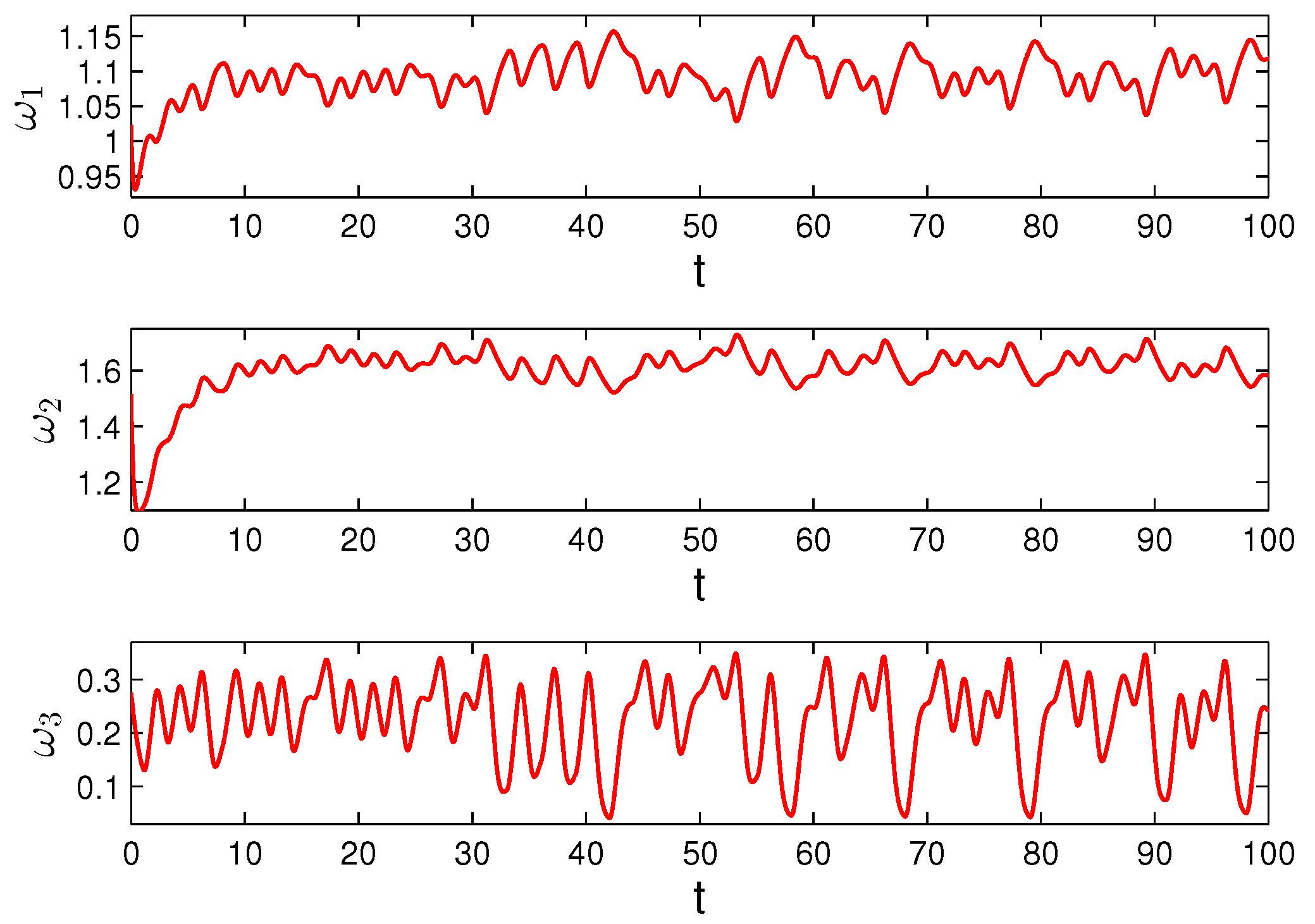
and $v_1\left(t\right)=-58{\Theta }^3\left(t\right)+5,$ $v_2\left(t\right)=76{\Theta }^3+4,$ $v_3\left(t\right)=42\Theta \left(t\right)-3.$ The function $v\left(t\right)=(v_1\left(t\right),v_2\left(t\right),v_3\left(t\right))$ is unpredictable in accordance with Lemmas 3 and 4. The conditions (C1)–(C8) hold for the network (23) with ${\xi }_1={\xi }_2=2, {\xi }_3=3,$ ${\zeta }_1={\zeta }_2=4, {\zeta }_3=4.4,$ $L=0.35,$ $M_f=0.56,$ $H=2.$ It is not difficult to calculate that $L_F=0.57,\lambda =1.47.$ Consequently, there exists the unpredictable solution, $\phi \left(t\right),$ of the system. Since it is not possible to indicate the initial value of the solution, we apply the property of asymptotic stability, since any solution from the domain ultimately approaches the unpredictable oscillation. That is, to visualize the behavior of the unpredictable oscillation, we consider the simulation of another solution. We shall simulate the solution $\omega \left(t\right)$ with initial conditions ${\omega }_1\left(0\right)=1.023,$ ${\omega }_2\left(0\right)=1.516,$ ${\omega }_3\left(0\right)=0.275.$

Utilizing (20), we have that

$$\begin{array}{ccc}& & {\parallel \phi \left(t\right)-\omega \left(t\right)\parallel }_1\le {\parallel \phi \left(0\right)-\omega \left(0\right)\parallel }_1{e}^{(L_F-\lambda )t}<2H{e}^{(L_F-\lambda )t}\le 4e^{-0.9t},t\ge 0.\hfill \end{array}$$

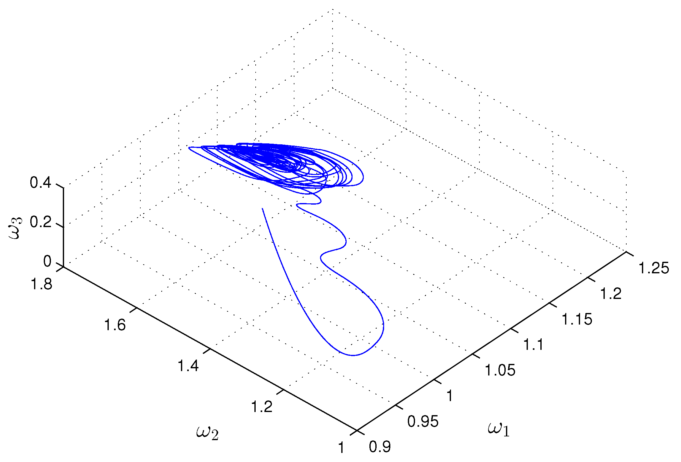
Thus, if ${\displaystyle t>\frac{9}{10}(5ln10+ln4)\approx 11.77,}$ then ${\parallel \phi \left(t\right)-\omega \left(t\right)\parallel }_1<{10}^{-5},$ and we can say that the graphs of the functions match visually, since they have technical conditions [37]. In other words, what is seen in Figure 1 and Figure 2 for a sufficiently large time can be accepted as parts of the graph and trajectory of the unpredictable solution. Both of the figures reveal the irregular dynamics of system (23).

5. Conclusions

We believe that the theorem that has been proved in the paper creates new circumstances in neuroscience, when extension, control, synchronization, and stabilization of periodic motions in chaotic dynamics can be realized more effectively than by conservative methods. The results are suitable for numerical simulations, and the dynamics can be subdued for more extended numerical analysis similar to the Lyapunov exponents evaluation and bifurcation diagram construction. The huge area of applications for the present research suggestions are nonlinear neural networks. For these models, the averaging method and different types of fixed point theorems can be utilized.

Application of the approach suggested in the present research can be effective with respect to different inertial mechanisms for dynamical systems and artificial neural networks. One can consider the applicability in the light of fractional human models [21] as well as artificial neural networks for uncertainly prediction [24], modeling the human driver [25], decision-making [26], classification [22], and machine translation [23].

References

- Ge, J.; Xu, J. Weak resonant double Hopf bifurcations in an inertial four-neuron model with time delay. Int. J. Neural Syst. 2012, 22, 22–63. [Google Scholar] [CrossRef]
- Ke, Y.Q.; Miao, C.F. Stability analysis of BAM neural networks with inertial term and time delay. WSEAS Trans. Syst. 2011, 10, 425–438. [Google Scholar]
- Ke, Y.Q.; Miao, C.F. Stability and existence of periodic solutions in inertial BAM neural networks with time delay. Neural Comp. Appl. 2013, 23, 1089–1099. [Google Scholar]
- Qi, J.; Li, C.; Huang, T. Stability of inertial BAM neural network with time-varying delay via impulsive control. Neurocomputing 2015, 161, 162–167. [Google Scholar] [CrossRef]
- Zhang, Z.; Quan, Z. Global exponential stability via inequality technique for inertial BAM neural networks with time delays. Neurocomputing 2015, 151, 1316–1326. [Google Scholar] [CrossRef]
- Zhang, W.; Huang, T.; Li, C.; Yang, J. Robust Stability of Inertial BAM Neural Networks with Time Delays and Uncertainties via Impulsive Effect. Neural Process. Lett. 2018, 44, 245–256. [Google Scholar] [CrossRef]
- Ke, Y.Q.; Miao, C.F. Stability analysis of inertial Cohen–Grossberg-type neural networks with time delays. Neurocomputing 2013, 117, 196–205. [Google Scholar] [CrossRef]
- Yu, S.; Zhang, Z.; Quan, Z. New global exponential stability conditions for inertial Cohen–Grossberg neural networks with time delays. Neurocomputing 2015, 151, 1446–1454. [Google Scholar] [CrossRef]
- Babcock, K.L.; Westervelt, R.M. Stability and dynamics of simple electronic neural networks with added inertia. Phys. D Nonlinear Phenom. 1986, 23, 464–469. [Google Scholar] [CrossRef]
- Rakkiyappan, R.; Premalatha, S.; Chandrasekar, A.; Cao, J. Stability and synchronization analysis of inertial memristive neural networks with time delays. Cogn. Neurodyn. 2016, 10, 437–451. [Google Scholar] [CrossRef] [Green Version]
- Rakkiyappan, R.; Gayathri, D.; Velmurugan, G.; Cao, J. Exponential Synchronization of Inertial Memristor-Based Neural Networks with Time Delay Using Average Impulsive Interval Approach. Neural Process. Lett. 2019, 50, 2053–2071. [Google Scholar] [CrossRef]
- Qin, S.; Gu, L.; Pan, X. Exponential stability of periodic solution for a memristor-based inertial neural network with time delays. Neural Comp. Appl. 2020, 32, 3265–3281. [Google Scholar] [CrossRef]
- Ramya, C.; Kavitha, G.; Shreedhara, K.S. Recalling of images using Hopfield neural network model. arXiv 2011, arXiv:1105.0332. [Google Scholar]
- Raiko, T.; Valpola, H. Oscillatory neural network for image segmentation with based competition for attention. Adv. Exp. Med. Biol. 2011, 718, 75–85. [Google Scholar] [PubMed] [Green Version]
- Schmidt, H.; Avitabile, D.; Montbrio, E.; Roxin, A. Network mechanisms underlying the role of oscillations in cognitive tasks. PLoS Comput. Biol. 2018, 14, e1006430. [Google Scholar] [CrossRef] [PubMed]
- Koepsell, K.; Wang, X.; Hirsch, J.; Sommer, F. Exploring the function of neural oscillations in early sensory systems, second edition. Front. Neurosci. 2010, 4, 53. [Google Scholar]
- Maguire, M.; Abel, A. What changes in neural oscillations can reveal about developmental cognitive neuroscience: Language development as a case in point. Develop. Cogn. Neurosci. 2013, 6, 125–136. [Google Scholar] [CrossRef] [Green Version]
- Hart, J.; Roy, R.; Muller-Bender, D.; Otto, A.; Radons, G. Laminar chaos in experiments: Nonlinear systems with time-varying delays and noise. Phys. Rev. Lett. 2019, 123, 154101. [Google Scholar] [CrossRef]
- Korn, H.; Faure, P. Is there chaos in the brain? II. Experimental evidence and related models. Neurosci. C. R. Biol. 2003, 326, 787–840. [Google Scholar] [CrossRef]
- Lassoued, A.; Boubaker, O.; Dhifaoui, R.; Jafari, S. Experimental observations and circuit realization of a jerk chaotic system with piecewise nonlinear function. In Recent Advances in Chaotic Systems and Synchronization; Boubaker, O., Jafari, S., Eds.; Elsevier: San Diego, CA, USA, 2019; pp. 3–21. [Google Scholar]
- Martínez-García, M.; Zhang, Y.; Gordon, T. Memory Pattern Identification for Feedback Tracking Control in Human–Machine Systems. Hum. Factors 2019. [Google Scholar] [CrossRef] [Green Version]
- Sharma, N.; Gedeon, T. Artificial Neural Network Classification Models for Stress in Reading. In ICONIP 2012: Neural Information Processing; Springer: Berlin/Heidelberg, Germany, 2012; pp. 388–395. [Google Scholar]
- Costa-juss‘a, M.R. From Feature to Paradigm: Deep Learning in Machine Translation. J. Artif. Intell. Res. 2018, 61, 947–974. [Google Scholar] [CrossRef]
- Kasiviswanathan, K.S.; Sudheer, K.P.; He, J. Quantification of prediction uncertainty in artificial neural network models. In Artificial Neural Network Modelling; Shanmuganathan, S., Samarasinghe, S., Eds.; Springer: Cham, Switzerland, 2016; pp. 145–159. [Google Scholar]
- MacAdam, C.C. Understanding and modeling the human driver. Veh. Syst. Dyn. 2003, 40, 101–134. [Google Scholar] [CrossRef]
- Hui, P.C.L.; Choi, T.-M. Using artificial neural networks to improve decision-making in apparel supply chain systems. In Information Systems for the Fashion and Apparel Industry; Choi, T.-M., Ed.; Woodhead Publishing: Sawston, UK, 2016; pp. 97–107. [Google Scholar]
- Akhmet, M.; Fen, M.O. Poincaré chaos and unpredictable functions. Commun. Nonlinear Sci. Nummer. Simul. 2017, 48, 85–94. [Google Scholar] [CrossRef] [Green Version]
- Akhmet, M.; Fen, M.O. Non-autonomous equations with unpredictable solutions. Commun. Nonlinear Sci. Nummer. Simul. 2018, 59, 657–670. [Google Scholar] [CrossRef]
- Akhmet, M.; Seilova, R.D.; Tleubergenova, M.; Zhamanshin, A. Shunting inhibitory cellular neural networks with strongly unpredictable oscillations. Commun. Nonlinear Sci. Numer. Simul. 2020, 89, 105287. [Google Scholar] [CrossRef]
- Akhmet, M.; Fen, M.O. Unpredictable points and chaos. Commun. Nonlinear Sci. Nummer. Simul. 2016, 40, 1–5. [Google Scholar] [CrossRef] [Green Version]
- Akhmet, M.; Fen, M.O. Existence of unpredictable solutions and chaos. Turk. J. Math. 2017, 41, 254–266. [Google Scholar] [CrossRef]
- Miller, A. Unpredictable points and stronger versions of Ruelle–Takens and Auslander—Yorke chaos. Topol. Appl. 2019, 253, 7–16. [Google Scholar] [CrossRef]
- Thakur, R.; Das, R. Strongly Ruelle-Takens, strongly Auslander-Yorke and Poincaré chaos on semiflows. Commun. Nonlinear. Sci. Numer. Simul. 2019, 81, 105018. [Google Scholar] [CrossRef]
- Akhmet, M.; Fen, M.O.; Tleubergenova, M.; Zhamanshin, A. Unpredictable solutions of linear differential and discrete equations. Turk. J. Math. 2019, 43, 2377–2389. [Google Scholar] [CrossRef]
- Akhmet, M.; Tleubergenova, M.; Zhamanshin, A. Poincare chaos for a hyperbolic quasilinear system. Miskolc Math. Notes 2019, 20, 33–44. [Google Scholar] [CrossRef]
- Driver, R.D. Ordinary and Delay Differential Equations; Springer Science Business Media: New York, NY, USA, 2012. [Google Scholar]
- Moor, H. MATLAB for Engineers, 3rd ed.; Pearson: London, UK, 2012. [Google Scholar]
Figure 1.
The coordinates of the function which exponentially converge to the coordinates of the unpredictable solution of Equation (23).
Figure 2.
The irregular trajectory of the solution
Publisher’s Note: MDPI stays neutral with regard to jurisdictional claims in published maps and institutional affiliations. |
© 2020 by the authors. Licensee MDPI, Basel, Switzerland. This article is an open access article distributed under the terms and conditions of the Creative Commons Attribution (CC BY) license (http://creativecommons.org/licenses/by/4.0/).
Share and Cite
MDPI and ACS Style
Akhmet, M.; Tleubergenova, M.; Zhamanshin, A. Inertial Neural Networks with Unpredictable Oscillations. Mathematics 2020, 8, 1797. https://doi.org/10.3390/math8101797
AMA Style
Akhmet M, Tleubergenova M, Zhamanshin A. Inertial Neural Networks with Unpredictable Oscillations. Mathematics. 2020; 8(10):1797. https://doi.org/10.3390/math8101797
Chicago/Turabian StyleAkhmet, Marat, Madina Tleubergenova, and Akylbek Zhamanshin. 2020. "Inertial Neural Networks with Unpredictable Oscillations" Mathematics 8, no. 10: 1797. https://doi.org/10.3390/math8101797
Note that from the first issue of 2016, this journal uses article numbers instead of page numbers. See further details here.