A Comparative Performance Evaluation of Classification Algorithms for Clinical Decision Support Systems


1
Data Science Group, Center for Mathematical and Computational Sciences, Institute for Basic Science (IBS), Daejeon 34141, Korea
2
Department of Industrial Engineering, Ulsan National Institute of Science and Technology, Ulsan 44919, Korea
*
Author to whom correspondence should be addressed.
Mathematics 2020, 8(10), 1814; https://doi.org/10.3390/math8101814
Submission received: 8 September 2020
/
Revised: 1 October 2020
/
Accepted: 6 October 2020
/
Published: 16 October 2020
(This article belongs to the Special Issue Recent Advances in Data Mining and Their Applications)
Abstract
:Classification algorithms are widely taken into account for clinical decision support systems. However, it is not always straightforward to understand the behavior of such algorithms on a multiple disease prediction task. When a new classifier is introduced, we, in most cases, will ask ourselves whether the classifier performs well on a particular clinical dataset or not. The decision to utilize classifiers mostly relies upon the type of data and classification task, thus making it often made arbitrarily. In this study, a comparative evaluation of a wide-array classifier pertaining to six different families, i.e., tree, ensemble, neural, probability, discriminant, and rule-based classifiers are dealt with. A number of real-world publicly datasets ranging from different diseases are taken into account in the experiment in order to demonstrate the generalizability of the classifiers in multiple disease prediction. A total of 25 classifiers, 14 datasets, and three different resampling techniques are explored. This study reveals that the classifier that is likely to become the best performer is the conditional inference tree forest (cforest), followed by linear discriminant analysis, generalize linear model, random forest, and Gaussian process classifier. This work contributes to existing literature regarding a thorough benchmark of classification algorithms for multiple diseases prediction.
1. Introduction
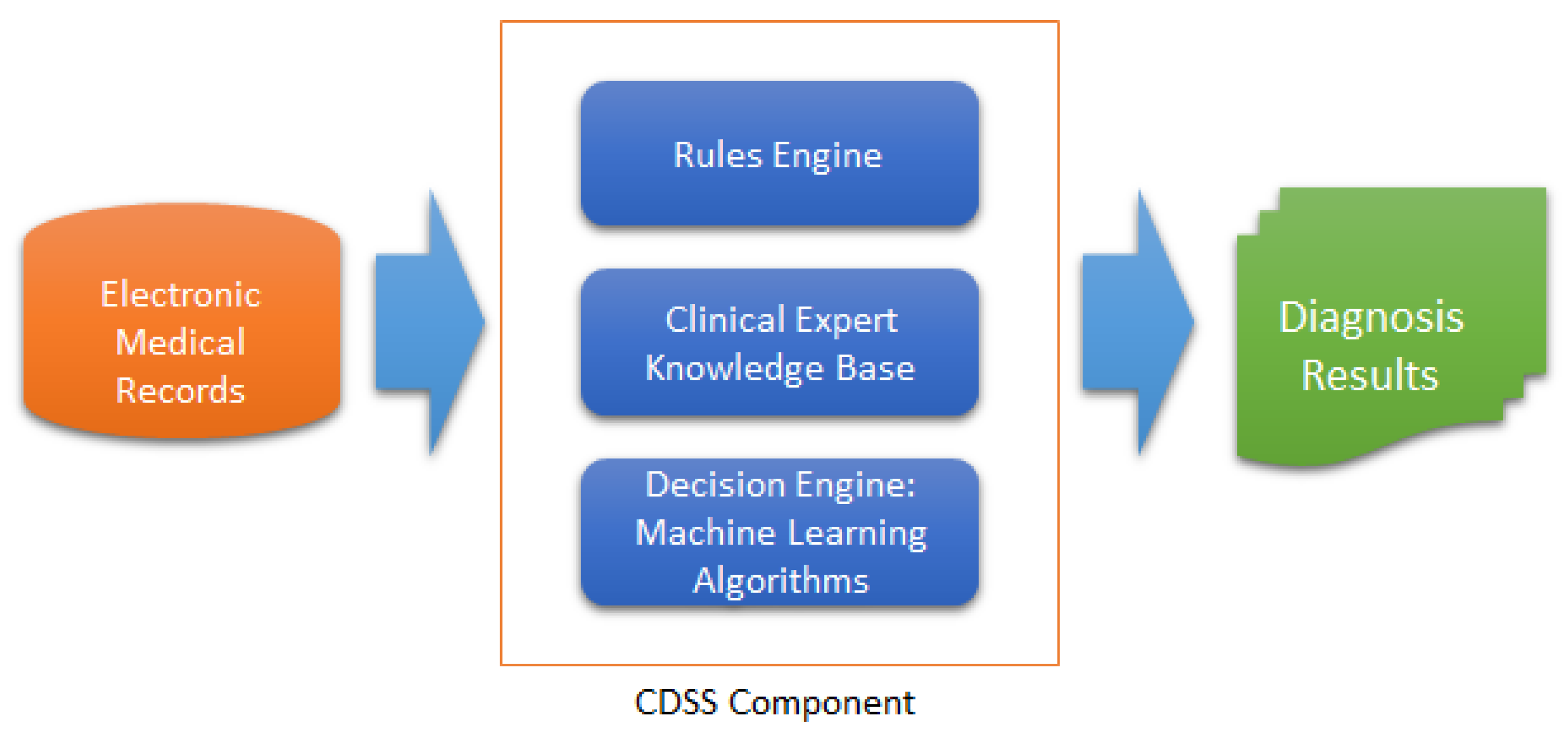
Artificial intelligence (AI) has changed almost all aspects of our lives dramatically. Undoubtedly, it will not be surprising that manpower is likely to be replaced by AI shortly owing to the rapid development of AI. Some AI techniques, e.g., deep learning and other machine learning (ML) algorithms, have been employed in clinical applications to support an intelligent system for an early detection and diagnosis method of disease [1]. Furthermore, they assist physicians in providing the second opinion about an effective clinical diagnosis, prognosis, and other clinical-related decision tasks in order to avoid potential human errors that might bring the patient life into risk [2,3]. Figure 1 illustrates how ML algorithms are employed in a clinical decision support system (CDSS).
With the emergence of new technological advancement, a large amount of clinical data has been stored and is ready for being analyzed by the clinical researchers. For instance, a large scale of clinical data are publicly available about patients admitted to critical care units at a large tertiary care hospital [4]. Nevertheless, most physicians are still suffering from an inaccurate prediction of a disease outcome due to a lack of knowledge about the available data analytics approaches. This condition leads to a significant improvement necessity of disease prediction using advanced ML techniques. For this reason, ML techniques have grown as a well-known tool for discovering and characterizing complex patterns and relationships among them from large datasets [5].
The prediction task could be either a classification or regression techniques, relying on the type of the target variable, i.e., categorical or numerical. In contrast, the task can be categorized into two main natures, i.e., predictive and descriptive [6,7,8]. A predictive task deals with inferring a function from a set of labeled training samples by mapping data samples based on input–output pairs. Such a task is also known as learning data in a supervised manner. Neural network, classification/regression trees, and support vector classifier/regressor are examples of supervised learning algorithms. In contrast, descriptive task algorithms, e.g., clustering and association techniques, attempt to make an inference from an unlabeled input data. The goal of these approaches is to group the objects into clusters or to figure out some interesting patterns between variables in databases. Examples of these techniques include K-means clustering, hierarchical clustering, and frequent itemset rule extractors.
Among those approaches mentioned above, the classification of clinical data is a very problematic task since it might be confusing to choose the best performing classifiers available in the wild. One of the causes is that the classifiers have emerged from different families, i.e., ensembles, decision trees, rule-based, Bayesian, and neural network, to name a few. A researcher might choose the classifiers erratically due to a limited knowledge within his/her competence or point of interest. Moreover, it would be a very challenging effort as each dataset is not likely to be uniform, considering that disease type and other clinical context domains might vary immeasurably in practice. Hitherto, having a particular prediction method does not always give a significant level of accuracy under all clinical application domains because it mainly relies on the context used. To be more precise, no one can guarantee that the proposed classifier will have a good performance in all clinical datasets unless an empirical benchmark is conducted [9].
Instead of simply conducting a qualitative analysis by using a systematic mapping study about previously published works [2,6,10,11,12], this study focuses on a quantitative analysis of classification techniques for disease prediction. This empirical study helps researchers and practitioners in deciding the best classification algorithms in a clinical application setting. It is the case that most researchers in the purview of medical informatics are solely familiar with specific ML techniques; thus, picking the best performing classifiers, in many cases, is a resource-intensive task. In addition, the performance of a new proposed classifier for clinical data analysis is often justified against the classifier within the restricted group, exempting the classifiers belonging to other groups. Hence, a cross-domain comparison of the ML algorithms from different groups for different diseases is currently unexplored. To the best of our knowledge, no other quantitative benchmark of ML algorithms that focuses on clinical data has been taken into consideration to date.
While some classification algorithms achieve a superior result with a given dataset, the performance of such classifiers might be contrasting on other datasets. The behavior of the classifiers is consistent with the no-free-lunch theorem [9], where there exists no single classifier or individual method that can be a panacea for all problems. Providing a classifier benchmark for multiple diseases, the objective of this empirical study is to originally find the excellent performing classifier across some clinical datasets. It is meant to assist researchers/practitioners about a reasonable decision in picking the available classifiers for clinical prediction, enabling them to determine a possible well-performing classifier.
According to the above-mentioned issues, this paper attempts to address the two following research questions (RQs):
- RQ: What is the relative performance of classification algorithms with respect to different resampling strategies?
- RQ: Among the various families, is there a best choice in selecting classification algorithm for clinical decision support systems?
2. Related Work
Huge research interest in a systematic mapping study currently exists [2,13,14], which aims at identifying and categorizing the prior published works in order to give a visual summary of their results. However, the approach is deemed to be an unreliable barometer for being taken as a guideline to find the best performing classifiers. This is because such an approach only serves a literature review concerning the most frequent use of ML techniques for clinical data analytics. For instance, Ref. Idri et al. [11] provided a systematic map of studies regarding the application of data processing in the healthcare domain, while a similar literature review of data mining methods for traditional medicine was reported in [15]. They have recognized that support vector machines and neural networks have always been used to solve the disease prediction task.
Jothi et al. [16] reviewed the various papers in the healthcare field with respect to methods, algorithms, and results. Garciarena and Santana [17] investigated the relationship between the type of missing data, the choice of imputation method, and the effectiveness of classification algorithms that employed the imputed data. Performance of several classification algorithms for early detection of liver disease was explored in [18]. The assessment results showed that C5.0 and CHAID algorithm were able to produce rules for liver disease prediction. Kadi et al. [6] had explored a systematic literature review of data mining techniques in cardiology, while Jain and Singh [19] focused their survey study on the utilization of feature selection and classification techniques for the diagnosis and prediction of chronic diseases.
More recently, Moreira et al. [20] analyzed and summarized the current literature of a smart decision support system for healthcare according to their taxonomy, application area, year of publication, and the approaches and technologies used. Sohail et al. [21] concluded that there is no an exclusive classifier or technique available to predict all kind of diseases. They overviewed the previous research that was applied in the healthcare industry. A particular ML technique, e.g., ensemble (meta) learning for breast cancer diagnosis, had been discussed in [10]. The research emphasized ensembles techniques applied to breast cancer data using a systematic mapping study. Lastly, Nayar et al. [22] explored various applications that utilized swarm intelligence with data mining in healthcare with respect to methods and results obtained.
It is worth mentioning that some existing works have performed a comparative study of classification techniques for the effective diagnosis of diseases. However, those studies are limited to either a particular disease or ML technique. This makes their studies still questionable with respect to its generalizability of the proposed methods in other clinical data with a different context. For instance, Das [23] employed multiple classification techniques, i.e., neural networks, regression, and decision tree for the diagnosis of Parkinson’s disease. Based on the experiment, a neural network classifier was found to be the best performing classifier with an accuracy of 92%. The proposed disease detection model, called ‘HMV,’ was taken into consideration to overcome the drawbacks of a traditional heterogeneous ensemble [24]. A similar approach, called ‘HM-BagMoov,’ was proposed to solve the limitations of conventional heterogeneous ensemble [25]. These two approaches were evaluated on a different number of clinical datasets, i.e., five heart datasets, four breast cancer datasets, two diabetes datasets, two liver disease datasets, and a hepatitis dataset.
To sum up, the aforementioned existing studies possess the following limitations:
- Most studies had simply reviewed previous publications by using a mapping study; thus, they could not be used as a support tool in providing a more informed choice to select the best performing classifier for disease prediction.
- When comparing multiple algorithms with multiple datasets, there existed a lack of statistical significance tests. Hence, the performance difference among the classification algorithms was still unrevealed.
In this study, a broad spectrum of classification algorithms, covering different groups, i.e., meta, tree, rule-based, neural, and Bayesian, are taken into consideration. A total of 25 classifiers are involved in the comparison. In addition, 14 real-world clinical datasets with different peculiarities are included in the benchmark. In order to see the impact of different sampling strategies on the classifier’s performance, we incorporate 3 different sampling techniques, i.e., subsampling, cross-validation, and multiple rounds of cross-validation. Finally, the results of some statistical significant tests are reported in order to prove that the performance classifier algorithms are significantly different, e.g., there is at least one algorithm that does not perform equal to the others.
3. Materials and Methods
In this section, several datasets that we employed in the experiment are presented, followed by a brief review of classification algorithms. Finally, significance tests are discussed in the last section.
3.1. Datasets
We mostly obtain the datasets from the UCI machine learning repository [26]. There are 12 real-world datasets that we download from the UCI website, while two datasets, i.e., RSMH [8] and Tabriz Iran [27] are privately available (can be obtained upon request). All datasets are categorized into seven different diseases, such as diabetes (4 datasets), breast cancer (3 datasets), heart attack (3 datasets), and one dataset for each thoracic, seizure, liver, and chronic kidney. Furthermore, some datasets hold several classes in their class label attributes; thus, they can be a multi-class classification problem. Such a case of Tabriz Iran [27], where the input variables can be classified into three classes, i.e., negative, positive, and old patient; Z-Alizadeh Sani [28] possess four class attributes, i.e., normal, stenosis of the left anterior descending (LAD) artery, left circumflex (LCX) artery, and right coronary artery (RCA); Cleveland, which predicts the input attributes as being in 4 classes, consisting of an integer value ranging from 0 (no heart disease) to 4 severe heart disease; and Epileptic Seizure Recognition, where the instances labeled class 1 are diagnosed with seizure disease and the instances having any of the classes 2, 3, 4, and 5 are specified as non-seizure disease subjects. The remaining datasets have a binary class in their response attribute. In this study, all datasets having multi-class targets were transformed into binary class targets with a specific criteria, i.e., the subjects labeled class 1 are diagnosed with the disease while they are 0, otherwise.
In the experiment, each dataset undergoes a simple pre-processing step, ensuring that the response attribute of each dataset is a categorical variable with two categories. Another pre-processing step, e.g., feature selection, is not carried out. This is because of the following reasons: (i) our aim is not to achieve the best possible performance of the classifier on each dataset, yet to benchmark algorithms on each dataset, (ii) the performance result of the classifier on a subset features might be random, and (iii) feature selection is usually made on each dataset, making a significant increase to the scope of this work. Any missing values in the datasets are treated using “do-nothing” strategy, meaning that we let some classification algorithms (e.g., gradient boosting machine (GBM) and a generalized linear model (GLM), etc.) to learn the best imputation values for the missing data (e.g., a mean imputation is typically used). However, other algorithms that do not tolerate missing values, an observation that has one or more missing values is simply dropped. Finally, for each dataset, a simple transformation is applied to ensure each dataset is ready to be processed by Weka and R. Table 1 summarizes the collection of 12 datasets from UCI repository and two datasets from privately clinical domains.
3.2. Classification Algorithms
Twenty-five classification algorithms implemented in R and are included in this study. These classifiers were chosen with respect to their previous performance behavior in the CDSS domain. Note that previous works have used a variety of classifiers, ranging from tree-based learners [18] to ensemble learners [10]. All classifiers implemented in R are accessible through package [39], while classifiers implemented in Weka [40] are run using a command-line of the class of each classifier. We briefly explain all classifiers as the following. All classifiers are grouped according to which family they particularly belong to. All default learning parameters are used in the experiment. For the sake of reproducibility, learning parameters of each classifier are listed in Appendix A.
- a.
- Tree-based algorithms: 5 learners
- i.
- C50 decision tree (C50)The classifier is the extension of the C4.5 algorithm presented in [41] that possesses extra improvements such as boosting, generating smaller trees, and unequal costs for different types of errors. Tree pruning is performed by a final global pruning strategy in which the costly and complex sub-trees are removed in such a way the error rate exceeds the baseline, e.g., the standard error rate of a decision tree without pruning. C50 can generate a set of rules, as well as a classification tree.
- ii.
- Credal decision tree (CDT)It takes into account imprecise probabilities and uncertainty measures for split criteria [42]. This procedure is a bit different from C4.5 or C50, where an information gain is used for a split criterion to choose the split attribute at each branching node in a tree.
- iii.
- Classification and regression tree (CART)It is trained in a recursive binary splitting manner to generate the tree. Binary splitting is a numerical process in which all the values are organized, and different split points are tested using a cost function. The split with the lowest cost is chosen [43].
- iv.
- Random tree (RT)It grows a tree using K randomly selected input features at each node without pruning. The cost function (error) is estimated during the training; thus, there is no accuracy estimation operation, i.e., cross-validation or train-test to obtain an estimate of the training error [44].
- v.
- Forest-PA (FPA)The classifier generates bootstrap samples from the training set and trains a CART classifier on the bootstrap sample using the weights of the attributes. The weights of the attributes are then updated incrementally that are presented in the latest tree. Following this step, the weights of applicable attributes are updated using their respective weight increment values that are not present in the latest tree [45].
- b.
- Ensemble methods: 7 learners
- i.
- Random forest (RF)It uses decision trees as a base classifier, while the tree is grown to a depth of one; then, the same procedure is replicated for all other nodes in the tree until the specified depth of the tree is reached [44].
- ii.
- Extra trees (XT)It works similarly to the random forest classifier, yet the features and splits are chosen at random; thus, it is also known as extremely randomized trees. Because splits are chosen at random, the computational cost (variance) of extra trees is lower than the random forest and decision tree [46].
- iii.
- Rotation forest (RoF)The classifier generates M feature subsets randomly and principal component analysis (PCA) is applied to each subset in order to restore a full feature set (e.g., using M axis rotations) for each base learner (e.g., decision tree) in the ensemble [47].
- iv.
- Gradient boosting machine (GBM)The classifier is proposed to improve the performance of the classification and regression tree (CART). It constructs an ensemble serially, where each new tree in the sequence is in charge of rectifying the prior tree’s prediction error [48].
- v.
- Extreme gradient boosting machine (XGB)The classifier is a state-of-the-art implementation of the gradient boosting algorithm. It shares a similar principle with GBM; however, less computational complexity is one of its advantages. In addition, XGB utilizes a more regularized model, making it able to reduce the complexity of the model while improving the prediction accuracy [49].
- vi.
- CForest (CF)The classifier differs from random forest in terms of the base classifier employed and the aggregation scheme implemented. It utilizes conditional inference trees as a base learner. At the same time, the aggregation scheme works by taking the average weights obtained from each tree, not by averaging predictions directly as the random forest does [50].
- vii.
- Adaboost (AB)The classifier attempts to improve the performance of a weak classifier, e.g., decision tree. The weak learner is trained sequentially on several bootstrap resamples of the learning set. Such a sequential scheme takes the results of a previous classifier into the next one to improve the final prediction by having the latter one emphasizing more on the mistakes of the earlier classifiers [51].
- c.
- Neural-based algorithms: 4 learners
- i.
- Deep learning (DL)It derives from a multilayer feed-forward neural network, which is built based on a stochastic gradient descent algorithm of back-propagation. The primary distinction from a conventional neural network is that it possesses a large number of hidden layers, e.g., greater than or equal to four layers. In addition, some fine-tuned hyper-parameters are needed to be set properly, where a grid search is an option for obtaining the best parameter settings [52].
- ii.
- Multilayer perceptron (MLP)The classifier is a fully connected feed-forward network, where the training is performed by error propagation method [53].
- iii.
- Deep neural network with a stacked autoencoder (SAEDNN)It is a deep learning classifier, where the weights are initialized by a stacked autoencoder [54]. Similar to a deep belief network, it is trained with a greedy layerwise algorithm, while reconstruction error is used as an objective function.
- iv.
- Linear support vector machine (SVM)A support vector machine works based on the principle of hyperplane that classifies the data in a higher dimensional space [55]. In this study, a linear implementation [56] is used with an -regularized and -loss descent method. This is because the linear implementation is computationally efficient as compared to LibSVM [57], for instance.
- d.
- Probability-based classifiers: 3 learners
- i.
- Naive Bayes (NB)A Naive Bayes classifier performs classification based on the conditional probability of a categorical class variable. It considers each of the variables to contribute independently to the probability [58]. In many application domains, the maximum likelihood method is prevalently considered for parameter estimation. Furthermore, it can be trained very efficiently in a supervised learning task.
- ii.
- Gaussian process (GP)A Gaussian process is defined by a mean and a covariance function. The function in any data modeling problem is considered to be a single sample in Gaussian distribution. In the classification task, the Gaussian process uses Laplace approximation for the parameter estimation [59].
- iii.
- Generalized linear model (GLM)The classifier can be used either for classification and regression tasks. In this study, a multinomial family generalization is used as we deal with multi-class response variables. It models the probability of an observation belonging to an output category given the data [60].
- e.
- Discriminant methods: 3 learners
- i.
- Linear discriminant analysis (LDA)The classifier assumes that any data model problem is Gaussian, and each attribute has the same variance. It estimates the mean and the variance for each class, while the prediction is made by estimating the probability of a test set belongs to each class. The output class is the one that gets the highest probability, in which the probability is estimated using Bayes theorem [61].
- ii.
- Mixture discriminant analysis (MDA)This classifier is an extension of linear discriminant analysis. It is used for classification based on mixture models, while the mixture of normals is employed to get a density estimation for each class [62].
- iii.
- K-nearest neighbor (K-NN)The classifier performs prediction on each row of the test set by finding the k nearest (measured by Euclidean distance) training set vectors. The classification is then made by majority voting with ties broken at random [63].
- f.
- Rule-based algorithm: 3 learners
- i.
- Repeated incremental pruning (RIP)This classifier was originally developed to improve the performance of the algorithm. The classifier constructs a rule by taking into account the following two procedures: (1) data samples are randomly divided into two subsets, i.e., a growing set and a pruning set, and (2) a rule is grown using the FOIL algorithm. After generating a rule, the rule is straightaway pruned by eliminating any final sequence of conditions from the rule [64]. In this study, we employ a Java implementation of the RIP algorithm, so-called JRIP.
- ii.
- Partial decision tree (PART)This classifier is a rule-induction procedure that avoids global optimization. It combines the two major rule generation techniques, i.e., decision tree (C4.5) and RIP. PART produces rule sets that are as accurate and of a similar size to those produced by C4.5, and more accurate than the RIP classifier [65].
- iii.
- OneR (1-R)This is a straightforward classifier that produces one rule for each predictor in the training set and selects the rule with a minimum total error as its final rule. A rule for a predictor is produced by generating a frequency table for each predictor feature against the target feature [66].
3.3. Resampling Procedures
Several different resampling procedures, i.e., subsampling, cross-validation, and multiple-round of cross-validation, are included in this study. The objective of using different resampling methods is to ensure that the performance of classifiers is not obtained randomly. A generic resampling procedure is illustrated in Algorithm 1 [67]. Subsampling is a repeated hold-out, where the original dataset is split into two disjoint parts with a specified proportion, i.e., in this study, 80% for the training set and 20% for the testing set. The procedure is then replicated ten times. Cross validation divides the dataset into k (10 in our case) equally disjoint parts (subsets) and employs k-1 parts to build the model, while the remaining part is used for validation. This step is repeated k rounds, where the test subset is different in each step. Lastly, multiple-round cross-validation is carried out by reproducing twofold cross-validation for five times. This procedure maintains the equal number of performance values as in the two other resampling procedures. We take the average value for each resampling procedure.
| Algorithm 1 General resampling strategy |
Input: A dataset of n observation to , the number of subsets k, and a loss function . Process: 1. Generate k subsets of named to 2. 3. for to k do 4. 5. 6. 7. 8. end 9. Aggregate , i.e., Output: Summary of validation statistics. |
3.4. Significance Tests
In order to demonstrate an extensive empirical evaluation of classifiers, it is essential to utilize statistical tests in order to verify the significant performance difference of classifiers that are measurable [68]. Several tests are briefly discussed as follows.
- A non-parametric Friedman test [69] is exploited to inspect whether there exist significant differences between the classifiers with respect to the performance metrics as mentioned earlier [70]. The null hypothesis (): no performance differences between classifiers exist, i.e., the expected difference that is equal to zero is observed against the alternative hypothesis (): at least one group of classifiers does not have the same performance, i.e., the expected difference is not equal to zero. The statistic of the Friedman test is calculated according to Equation (1):where v denotes the number of datasets (14 in our case), w denotes the number of classifiers (25 in our case) to be compared, and the average rank of classifier algorithm is .
- Finner test [71] is an p-value adjustment in a step-down manner. Let be the ordered p-values in increasing order, so that , and are the respective hypotheses. It rejects to if w is the smallest integer. Due to its simplicity and power, Finner test is a good choice in general.
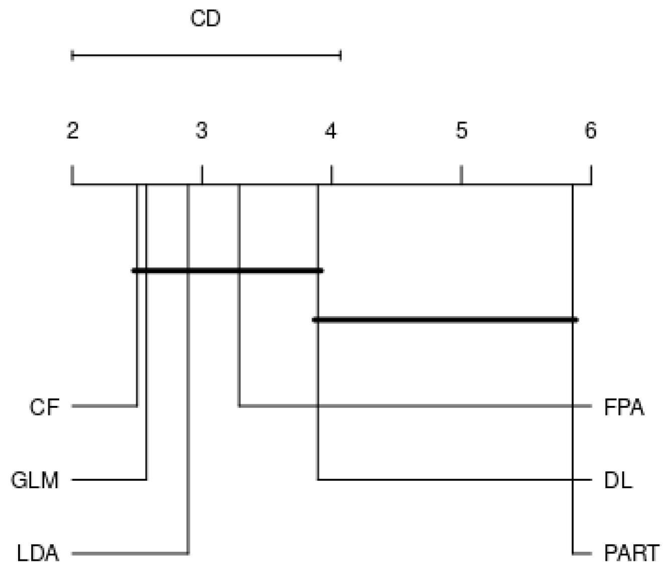
- Nemenyi test [72] works by calculating the average rank of each benchmarked algorithm and taking their differences. In case such average differences are larger than or equal to a critical difference (CD), the performances of the algorithms are significantly different. CD can be obtained using the following formula:where is the Studentized statistic divided by .
More specifically, the procedures of significance tests can be broken down as follows.
- Calculate the classifiers’ rank for each dataset using Friedman rank with respect to their area under ROC curve (AUC) metric in increasing order, from the best performer to the worst performer.
- Calculate the average rank of each classifier over all datasets. The best-performing classifier is determined by the lowest value of Friedman rank. Note that the merit is inversely proportional to numeric value.
- Calculate p-value using an omnibus test, e.g., Friedman.
- If the Friedman test demonstrates significant results (p-value < 0.05 in our case), run the Finner’s method. It is carried out based on a pairwise comparison, where the best-performing algorithm is used as a control algorithm for being compared with the remaining algorithms.
- Perform a Nemenyi test to compare the performance of classifiers by each family.
4. Results and Discussion
4.1. Overall Analysis
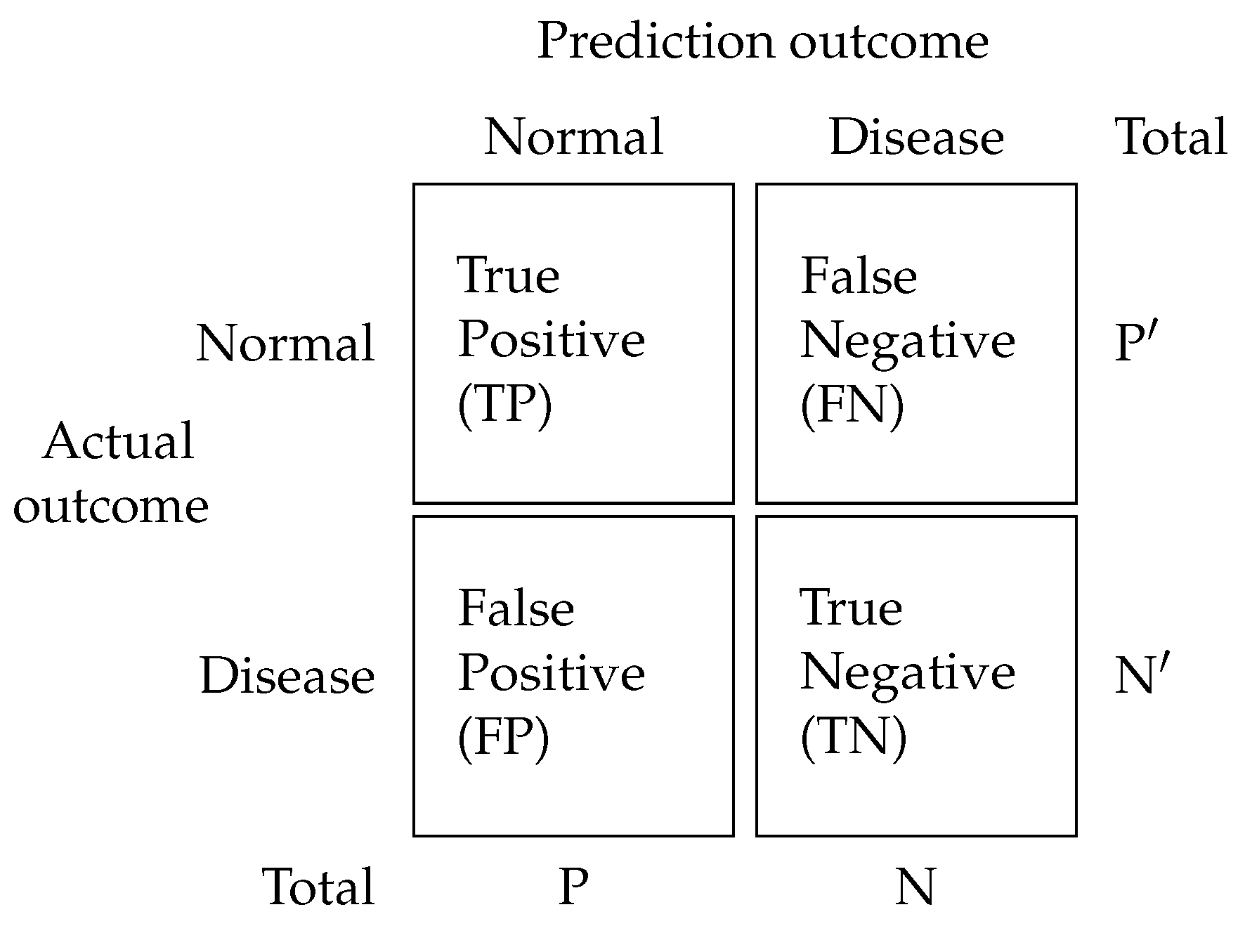
In this research, we implement 25 algorithms over 14 datasets and three different validation strategies, providing 1050 combinations of algorithm-datasets-validation methods. Three different validation procedures are taken into account to anticipate a poor bias and variance due to a small size of samples in each dataset. Furthermore, different validation procedures ensure that the experimental results were not obtained by chance. The test results are the average of 10 elements at each resampling method. All classifiers’ performance are assessed in terms of AUC metric. By referring the contingency table shown in Figure 2, AUC value of a classification algorithm can be calculated as:
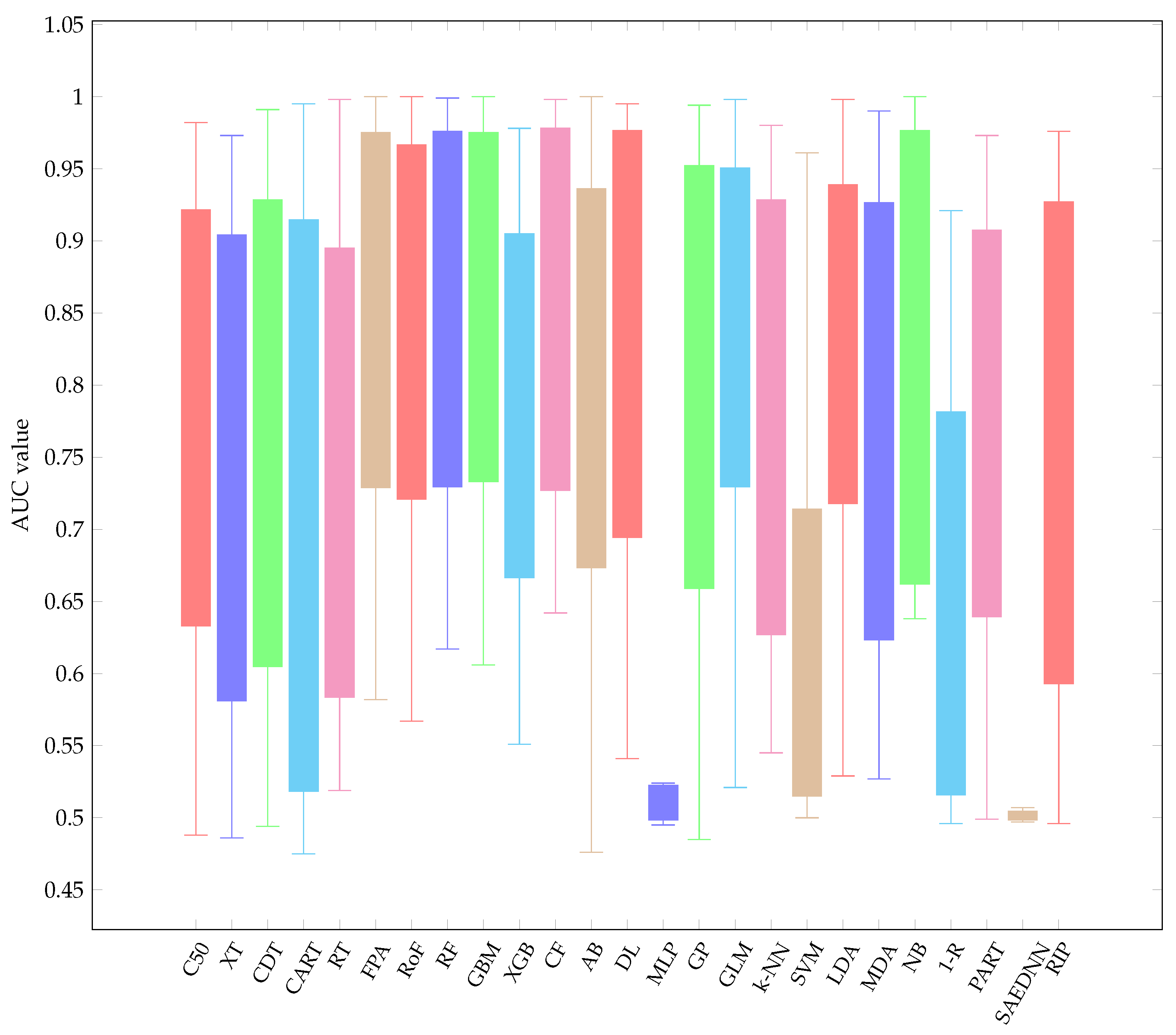
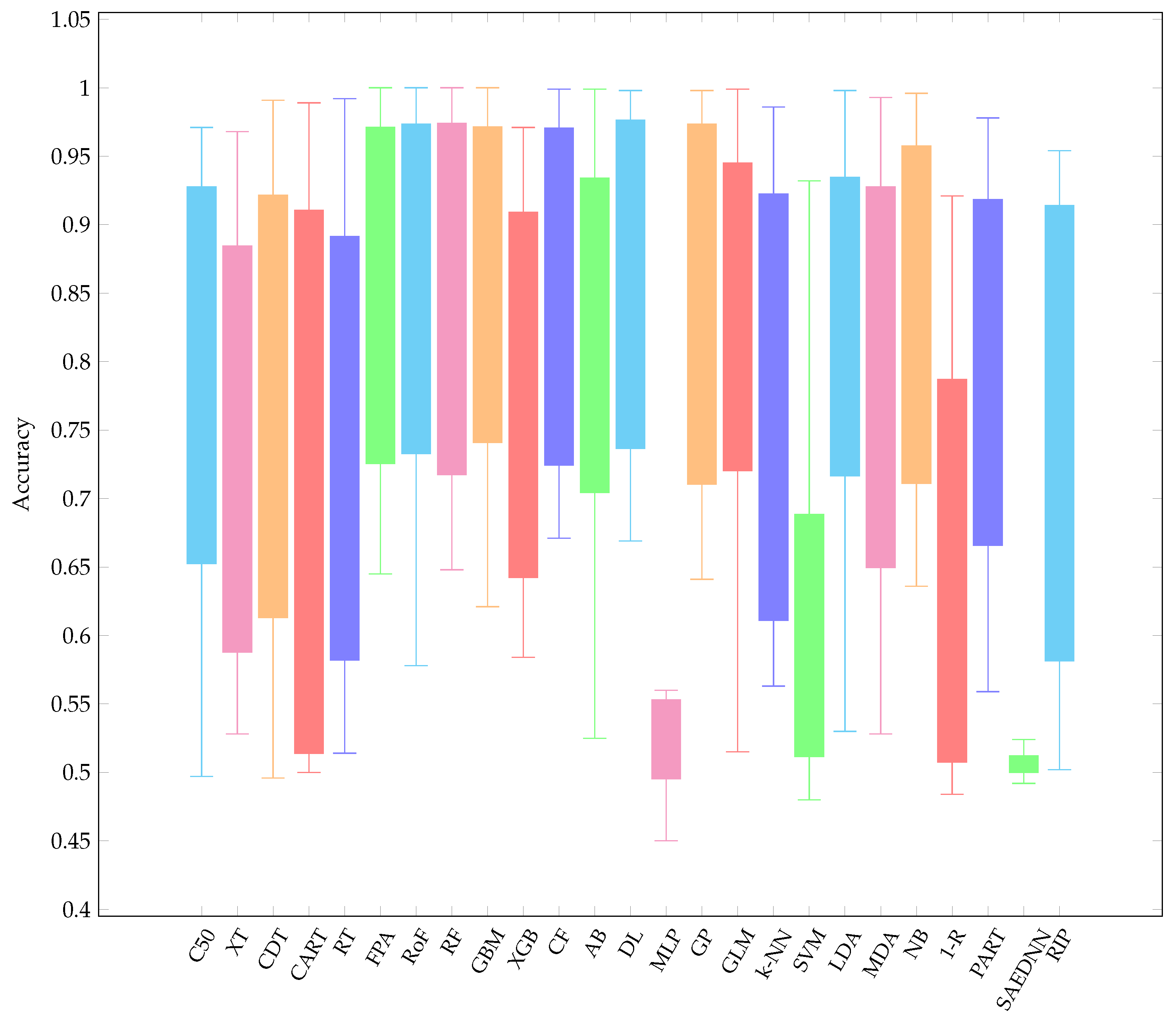
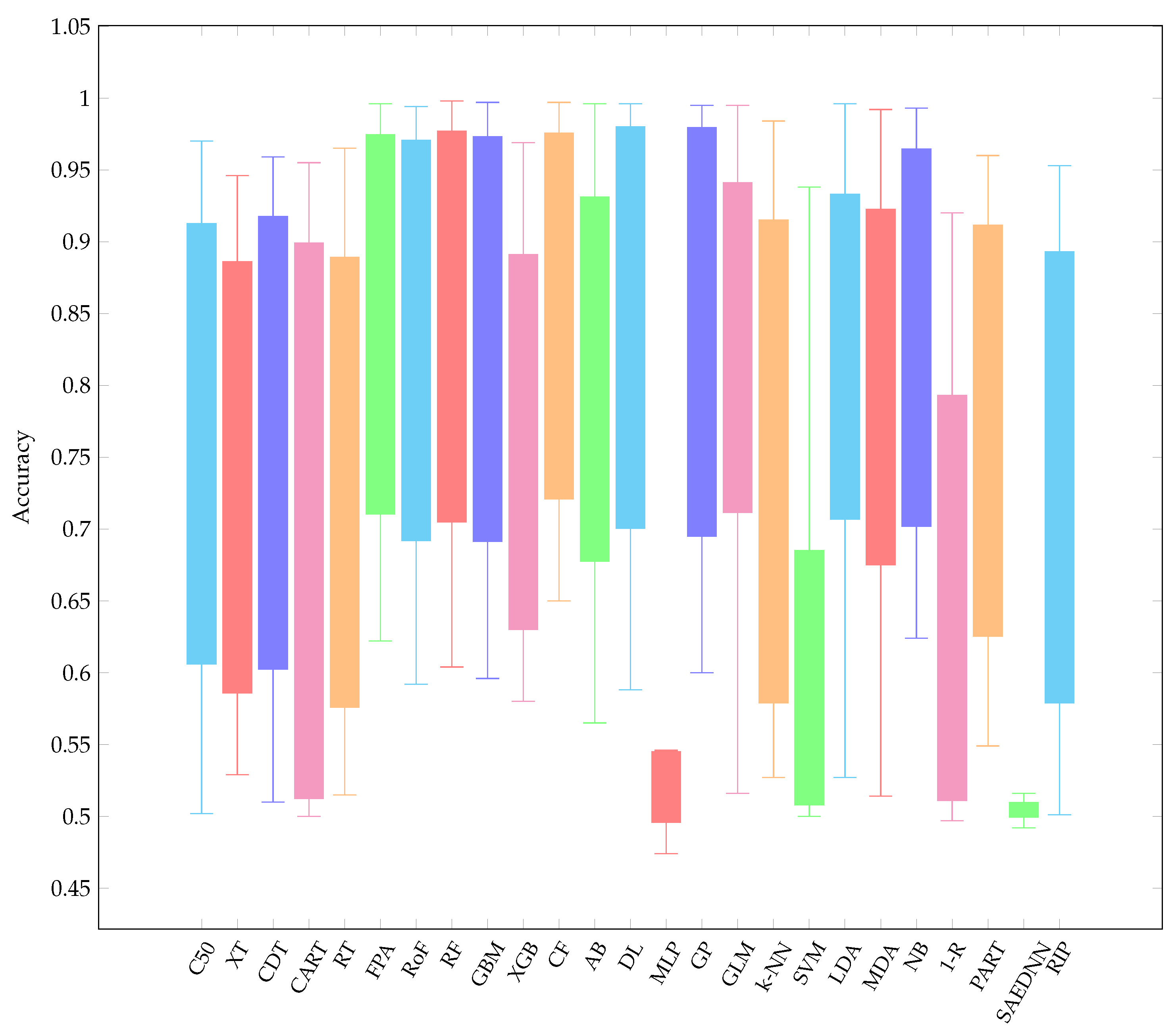
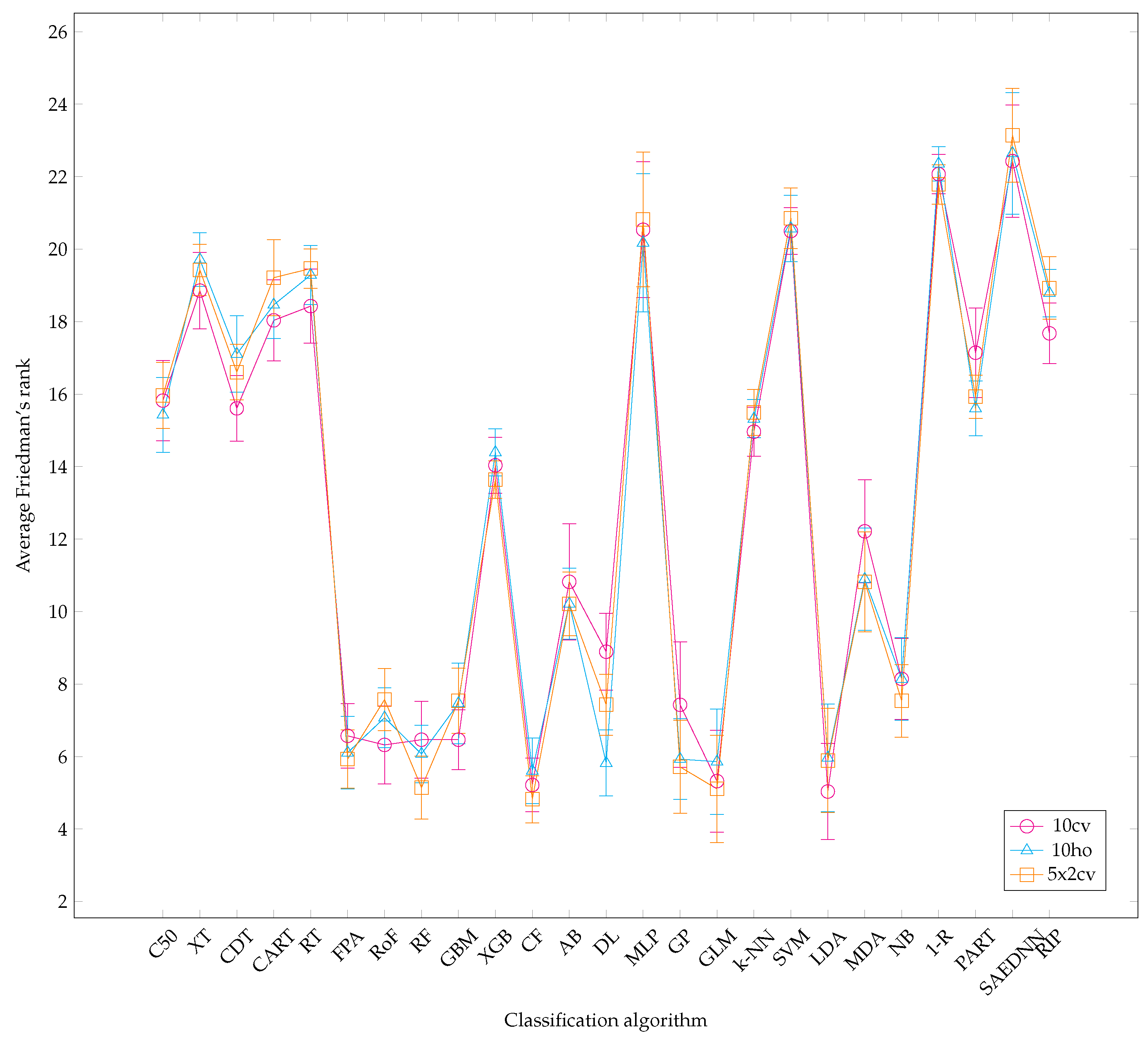
To maintain the readability of this paper, all performance results are provided in Appendix B. In Figure 3, Figure 4 and Figure 5, the AUC value of each classification algorithm for each validation method is firstly shown. The boxplots show the distributions of data according to the AUC values obtained for each dataset. More specifically, they indicate the performance variability of classification algorithms relative to each dataset. The mean AUC values are grouped based on each resampling technique. It can be observed that there is a greater variability for FPA, RoF, RF, GBM, SVM, LDA, AB, and 1-R, regardless of validation methods considered. On the other hand, MLP and SAEDNN have less variability, meaning that such classifiers’ performances are consistent, in spite of the clinical dataset used. Overall, the six best-performing algorithms (in descending order of mean AUC value) are apparently CF, RF, FPA, RoF, DL, and GBM. Furthermore, since simply taking the average performance value might lead to bias, a Friedman ranking is adopted for assessing the classifier’s performance (see Figure 6). Instead of analyzing the explicit performance, Friedman rank analysis is based on the rank of each classifier on each dataset. To address the RQ, we analyze the relative performance of classifiers in different resampling strategies using the Friedman rank. With reference to 10cv, the Friedman rank can confirm that the six top-performing classifiers, in ascending order, from the best-performer to the worst performer are LDA, CF, GLM, RoF, RF, and GBM with average rank 5.04, 5.21, 5.32, 6.32, 6.46, and 6.47, respectively.
According to Friedman rank and 10ho, the top-5 superior performers are CF, followed by DL, GLM, GP, and LDA with average rank 5.61, 5.82, 5.86, 5.93, and 5.96, respectively. Subsequently, with respect to 5 × 2cv, CF is on the topmost performance with average rank 4.82. This is succeeded by GLM, RF, GP, and LDA, with average rank 5.11, 5.14, 5.71, and 5.89, respectively. For the sake of an inclusive evaluation, the behavior of the top-performing classifiers can be discussed as follows:
- Overall, it is worth mentioning that, over the three resampling techniques, CF have performed best with average AUC 0.857 and rank 5.16. The result is reasonably unexpected since a conditional inference tree model can outperform other gradient-based ensemble algorithms, i.e., XGB.
- CF is as good as RF since CF works similar to RF [73]. Therefore, it is not surprising that both CF and RF are not significantly different.
- Other ensemble learners, i.e., RF and RoF have performed better than other ensemble models, i.e., FPA and XGB.
- Regarding a highly performance of RF, it is obvious that RF is built based on an ensemble of decision trees. The randomness of each tree split usually provides better prediction performance. In addition, RF is resilient in order to deal with imbalance datasets [74]. Note that several datasets employed in this experiment are highly imbalanced (see Table 1).
- LDA is listed in the top-5 best performing classifiers. LDA has been known as a simple but robust predictor when the dataset is linearly separable.
Based on our experimental results, the worst performer over three resampling techniques is SAEDNN with average rank 22.74 and average AUC 0.538. This is not surprising because a deep neural network always requires a large number of training samples to build the model. Moreover, neural-based classifiers are nonlinear classifiers, meaning that they are more affected by some hyperparameter-tuning such as learning rate, epochs, number of hidden layers, etc. The lowest AUC might also be the result of an insufficiency of training data samples when constructing the classification model. Moreover, it can be observed that the second and the third worst models are 1-R, SVM, and MLP.
A post-hoc test, i.e., Finner, is carried out after an omnibus Friedman test. If the Friedman test rejects the null hypothesis (there is no performance difference in at least one of the classifiers and others), the post-hoc test is applied. The result of statistical significance tests for each resampling technique is given in Table 2, Table 3 and Table 4. Concerning the post-hoc test, several options are prevalently available such as a pair-wise comparison, comparison with control classifier, and all pair-wise comparisons. In this study, all pair-wise comparison is adopted. The p-value < 0.01 is set as a significant threshold. The results of Table 2, Table 3 and Table 4 are further discussed. According to Finner test, low-performing classifiers, i.e., RIP, SAEDNN, SVM, and MLP are significantly different compared to the rest algorithms. In order to inspect how the three resampling procedures have an impact on the classifier’s performance, we extend our comparative analysis in the following section.
4.2. Analysis by Each Family
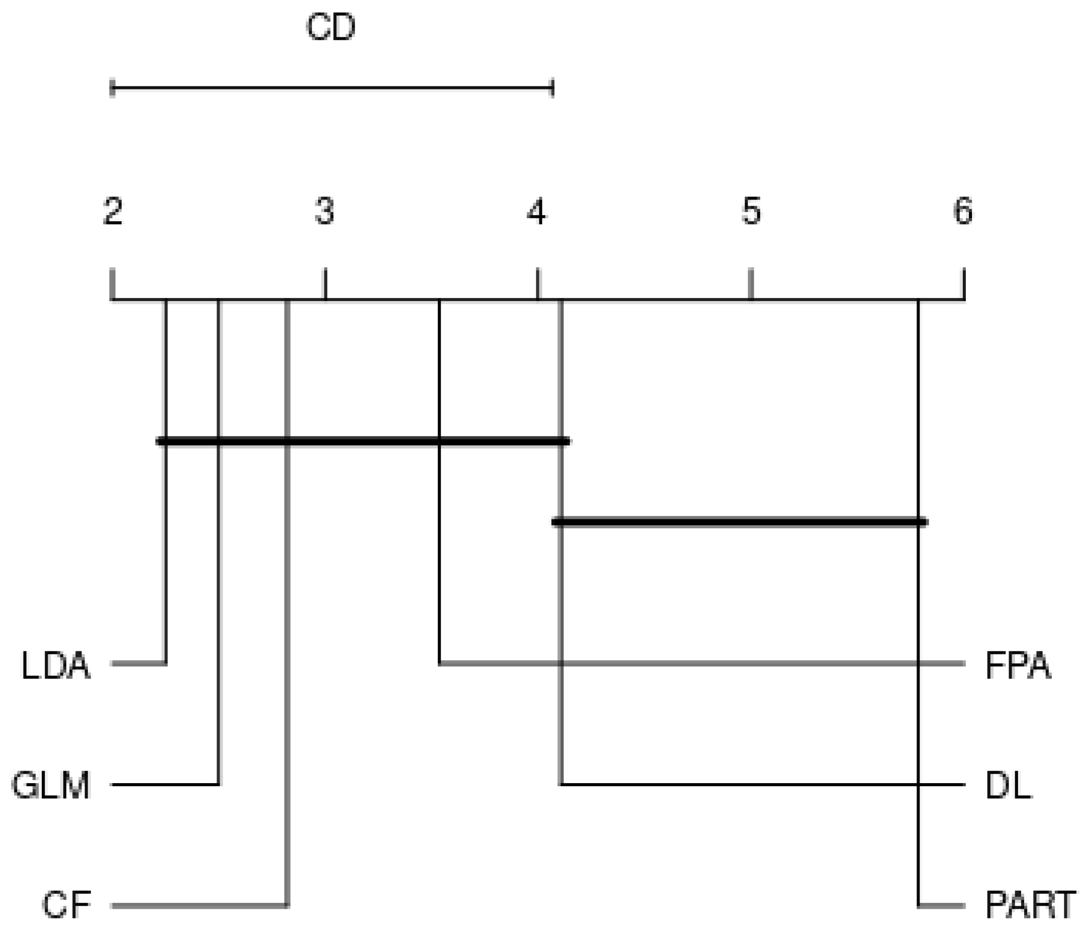
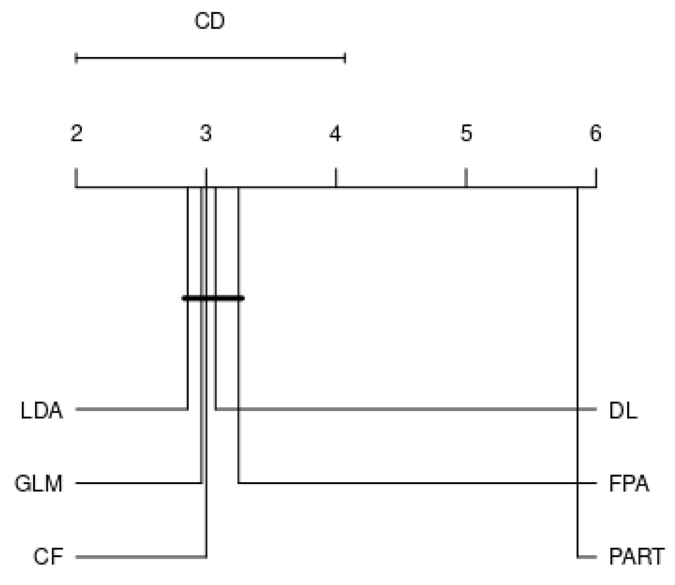
In this section, in order to answer RQ, we focus on the benchmark of best performing classifiers on each family, as well as the effect of different resampling strategies on the classifier’s performance. As a result, six top performers, corresponding to six different families, are included in the analysis. Among the tree-based classification algorithms, FPA is the best classifier, whilst CF and DL become the two leading classifiers among the ensemble and neural-based algorithms, respectively. GLM has performed best among the probability-based classifiers, whilst LDA is superior compared to other discriminant methods. Finally, PART is an outstanding classifier among the rule-based family. Figure 7, Figure 8 and Figure 9 expose the CD plots using the Nemenyi test for each resampling technique. It is obvious that, with respect to 10cv, PART and DL are significantly different than the rest of the algorithms since their rank is greater than the CD. The results of 10ho and 5 × 2cv are quite similar, where PART is the only algorithm that has a significant performance difference compared to the rest algorithms.
5. Conclusions
Rather than simply carrying out a mapping study, this study provided a more informed option about choosing the best classifier for disease prediction. This study demonstrated a thorough benchmark of 25 classification techniques corresponding to six families over 14 real-world disease datasets, as well as three different resampling procedures. Based on the experimental results, CF had shown its superiority in comparison with other classifiers. It achieved an average AUC 0.857 over all resampling techniques with an average Friedman rank is 5.16. The two worst performers, however, were from neural-based classifier family such as SAEDNN and MLP. These classifiers were not competitive since SAEDNN particularly required a sufficient training set to create the model. In general, the other top-4 classifiers that were very powerful for clinical decision support systems were LDA, GLM, RF, and GP. The following section presents the two RQs and provides answer to them.
- RQ: What is the relative performance of classification algorithms with respect to different resampling strategies? According to the Friedman rank, different resampling techniques had no significant impact on several classifiers.
- RQ: Among the various families, is there a best choice in selecting a classification algorithm for a clinical decision support system? This study revealed that choosing the classification algorithms for disease prediction highly depended on types of practical problems, i.e., imbalanced dataset, linear or nonlinear separable, and expert knowledge regarding data and domain. Therefore, it can be concluded that CF, LDA, GLM, RF, and GP were the best choices so far in clinical decision support system field since they are resilient to imbalanced datasets.
Among the potential approaches to extend this study, we believe that including more clinical datasets would be the most interesting since this might help researchers/clinical practitioners in selecting suitable classifiers in different application domains. For future work, it would be interesting to deal with the main drawback of this study about the performance AUC of state-of-the-art classifiers, i.e., XGB and SAEDNN. To this end, while a large amount of datasets are taken into consideration, the performance of deep structured learning might be improved. Taking into account that deep learning has played a significant role in classifying medical images, acoustic signals, or biosignals detected from medical devices, it would be meaningful to understand the performance of machine learning and deep learning applied on those clinical datasets.
Author Contributions
Conceptualization, B.A.T. and S.L.; methodology, B.A.T.; validation, B.A.T.; investigation, S.L.; writing—original draft preparation, B.A.T. and S.L.; writing—review and editing, B.A.T. and S.L.; visualization, B.A.T.; supervision, S.L.; funding acquisition, S.L. All authors have read and agreed to the published version of the manuscript.
Funding
This work was supported by the National Research Foundation of Korea (NRF) grant funded by the Korea government (MSIT) (No. 2019R1F1A1059346). This work was supported by the 2020 Research Fund (Project Number 1.180090.01) of UNIST (Ulsan National Institute of Science and Technology).
Conflicts of Interest
The authors declare no conflict of interest. The funders had no role in the design of the study; in the collection, analyses, or interpretation of data; in the writing of the manuscript, or in the decision to publish the results.
Appendix A. List of Learning Parameters Used in the Experiment
In the following, tuned parameters of 25 classifiers were briefly shown. Their names and implementations are specified using , where the implementation can be r (e.g., in R using ) and w (e.g., Weka).
- C50_rConfidence factor: 0.25; smallest number of samples: 2; fuzzy threshold: No; sample: 0.
- CDT_wk-th root attribute: 1; maximum tree depth: no restriction; minimum variance proportion: 0.001; imprecise Dirichlet model: 1.0.
- CART_wMinimal cost-complexity pruning: yes; number of folds in the internal cross-validation: 5; heuristic search for binary split: yes.
- RT_wMaximum depth of the tree: unlimited; the number of randomly chosen attributes: 0; amount of data used for backfitting: 0.
- FPA_wNumber of trees to build the forest: 100; number of pruning folds: 2; minimum number of objects: 2.
- RF_rThe implementation of HO is used. Number of trees to build the forest: 100; maximum depth of the tree: unlimited; number of randomly chosen attributes: 0; number of iterations: 100.
- XT_rMinimum number of instances required at a node: 2; number of attributes to randomly choose at a node: −1.
- RoF_wBase classifier: C4.5; number of iterations: 10; projection filter: principle component analysis.
- GBM_rThe implementation of HO is used. Fold assignment: Auto; number of trees: 100; maximum depth: 5; minimum observations in a leaf: 10; number of bins: 20; number of bins at the root level: 1024; number of bins for categorical columns: 1024; learning rate: 0.1; learning rate annealing: 1; sample rate: 1; column sample rate: 1; column sample rate per tree: 1; minimum split improvement: .
- XGB_rMaximum depth: 6; learning rate: 0.3; minimum sum of instance weight: 1; subsample ratio: 1; number of trees to grow per round: 1; number of trees: 100.
- CF_rThe argument: 5; number of trees: 100, minimum criterion: 0.
- AB_wNumber of instances to process: 100; base classifier: decision stump; number of iterations: 10; resampling is used: no; weight threshold for weight pruning: 100.
- DL_rThe implementation of HO is used. L1 and L2 regularization: 0; Hidden layer dropout ratio: 0.5; input dropout ratio: 0; number of training samples for which momentum increases: 1,000,000; learning rate decay: 1; learning rate annealing: ; learning rate: 0.005; adaptive learning rate smoothing factor: ; adaptive learning rate time decay: 0.99; adaptive rate: yes; number of epochs: 100; hidden layer sizes: c(200, 200), activation function: rectifier; maximum relative size of the training data: 5.
- MLP_rMaximum iterations: 100; number of units in the hidden layer: 200; learning function: standard backpropagation, parameter for the learning function: 0.2; activation function for hidden layer: logistic, number of hidden layer: 1.
- SAEDNN_rNumber of units in the hidden layers: 200; activation function: sigmoid; learning rate for gradient descent: 0.8; momentum rate for gradient descent: 0.5; learning rate scale: 1; number of epochs: 100, function of output unit: sigmoid; drop out fraction for hidden layer: 0, number of hidden layers: 2.
- SVM_wCost parameter: 1; bias: 1; : 0.001; parameter of the insensitive loss function: 0.1; number of iterations: 100.
- NB_wUse kernel estimator: no; use supervised discretization: no.
- GP_rData transformation: normalize training data; kernel type: polynomial kernel; exponent value: 1; level of Gaussian noise: 1.
- GLM_rFamily: Gaussian; tweedie variance power: 0; tweedie link power: 1; : ; solver: auto; : 0; number of lambdas to be used in a search: 100; missing value handling: mean imputation;
- LDA_rPrior: proportion; tolerance: ; degrees of freedom: t distribution.
- MDA_rNumber of iterations: 100; number of sub-classes per class: 3; regression method used in optimal scaling: polynomial regression.
- K-NN_wNumber of neighbours to use: 2; distance weighting method: no; nearest neighbours search method: Euclidean distance.
- RIP_wThe amount of data used for pruning: 3; minimum total weight: 2; number of optimizations: 2; use pruning: yes.
- PART_rConfidence factor: 0.25; the amount of data used for reduced-error pruning: 3; reduced-error pruning: no; binary splits: no; MDL correction: yes.
- 1-R_wThe minimum bucket size used for discretizing numeric attributes: 6.
Appendix B. Performance Results of All Benchmarked Classifiers

Table A1.
Performance results of all classification algorithms w.r.t. 10cv.
| DATASET | C50 | XT | CDT | CART | RT | FPA | RoF | RF | GBM | XGB | CF | AB | DL | MLP | GP | GLM | k-NN | SVM | LDA | MDA | NB | 1-R | PART | SAEDNN | RIP |
|---|---|---|---|---|---|---|---|---|---|---|---|---|---|---|---|---|---|---|---|---|---|---|---|---|---|
| Breast cancer (diagnostic) | 0.965 | 0.929 | 0.964 | 0.938 | 0.929 | 0.986 | 0.992 | 0.990 | 0.991 | 0.970 | 0.990 | 0.989 | 0.992 | 0.495 | 0.992 | 0.993 | 0.980 | 0.561 | 0.993 | 0.969 | 0.976 | 0.887 | 0.937 | 0.505 | 0.953 |
| Breast cancer (original) | 0.969 | 0.918 | 0.962 | 0.960 | 0.960 | 0.990 | 0.988 | 0.990 | 0.990 | 0.978 | 0.991 | 0.986 | 0.991 | 0.987 | 0.983 | 0.994 | 0.979 | 0.961 | 0.995 | 0.990 | 0.983 | 0.908 | 0.947 | 0.504 | 0.964 |
| Pima Indian | 0.784 | 0.647 | 0.779 | 0.727 | 0.684 | 0.823 | 0.833 | 0.817 | 0.809 | 0.783 | 0.829 | 0.801 | 0.777 | 0.497 | 0.832 | 0.832 | 0.717 | 0.596 | 0.832 | 0.796 | 0.819 | 0.649 | 0.794 | 0.499 | 0.734 |
| Statlog | 0.816 | 0.744 | 0.800 | 0.797 | 0.787 | 0.900 | 0.885 | 0.897 | 0.883 | 0.831 | 0.898 | 0.878 | 0.862 | 0.500 | 0.905 | 0.900 | 0.818 | 0.778 | 0.903 | 0.882 | 0.898 | 0.706 | 0.736 | 0.498 | 0.778 |
| Wisconsin prognostic | 0.602 | 0.486 | 0.494 | 0.475 | 0.579 | 0.629 | 0.730 | 0.617 | 0.741 | 0.682 | 0.642 | 0.695 | 0.696 | 0.497 | 0.640 | 0.739 | 0.617 | 0.504 | 0.792 | 0.722 | 0.642 | 0.504 | 0.500 | 0.487 | 0.638 |
| RSMH | 0.878 | 0.905 | 0.902 | 0.891 | 0.893 | 0.964 | 0.945 | 0.962 | 0.960 | 0.920 | 0.966 | 0.974 | 0.974 | 0.981 | 0.980 | 0.974 | 0.957 | 0.940 | 0.974 | 0.957 | 0.977 | 0.817 | 0.878 | 0.978 | 0.917 |
| Tabriz Iran | 0.558 | 0.557 | 0.545 | 0.529 | 0.569 | 0.754 | 0.712 | 0.708 | 0.720 | 0.663 | 0.720 | 0.727 | 0.680 | 0.503 | 0.724 | 0.721 | 0.545 | 0.500 | 0.721 | 0.534 | 0.753 | 0.499 | 0.613 | 0.502 | 0.528 |
| Thoracic surgery | 0.488 | 0.567 | 0.528 | 0.500 | 0.519 | 0.582 | 0.567 | 0.657 | 0.606 | 0.551 | 0.655 | 0.476 | 0.541 | 0.521 | 0.609 | 0.620 | 0.548 | 0.503 | 0.645 | 0.527 | 0.642 | 0.496 | 0.499 | 0.500 | 0.496 |
| Diabetic retinopathy | 0.683 | 0.616 | 0.665 | 0.668 | 0.616 | 0.731 | 0.821 | 0.754 | 0.770 | 0.668 | 0.770 | 0.652 | 0.786 | 0.508 | 0.764 | 0.768 | 0.648 | 0.643 | 0.796 | 0.761 | 0.682 | 0.528 | 0.694 | 0.499 | 0.637 |
| ILPD | 0.664 | 0.595 | 0.668 | 0.508 | 0.588 | 0.727 | 0.708 | 0.751 | 0.725 | 0.665 | 0.734 | 0.604 | 0.693 | 0.524 | 0.678 | 0.738 | 0.637 | 0.544 | 0.715 | 0.713 | 0.638 | 0.533 | 0.666 | 0.504 | 0.549 |
| Seizure | 0.966 | 0.903 | 0.955 | 0.942 | 0.897 | 0.990 | 0.995 | 0.995 | 0.995 | 0.890 | 0.992 | 0.898 | 0.979 | 0.505 | 0.485 | 0.521 | 0.900 | 0.609 | 0.529 | 0.528 | 0.984 | 0.746 | 0.950 | 0.505 | 0.937 |
| Chronic kidney | 0.982 | 0.973 | 0.991 | 0.995 | 0.998 | 1.000 | 1.000 | 0.999 | 1.000 | 0.969 | 0.998 | 1.000 | 0.995 | 0.687 | 0.994 | 0.998 | 0.970 | 0.689 | 0.998 | 0.966 | 1.000 | 0.921 | 0.973 | 0.500 | 0.976 |
| Cleveland | 0.806 | 0.752 | 0.809 | 0.810 | 0.710 | 0.898 | 0.900 | 0.904 | 0.892 | 0.823 | 0.906 | 0.894 | 0.882 | 0.501 | 0.904 | 0.902 | 0.841 | 0.739 | 0.904 | 0.896 | 0.894 | 0.724 | 0.773 | 0.507 | 0.810 |
| Z-Alizadeh | 0.764 | 0.748 | 0.838 | 0.799 | 0.638 | 0.914 | 0.893 | 0.919 | 0.900 | 0.823 | 0.924 | 0.898 | 0.892 | 0.506 | 0.924 | 0.927 | 0.828 | 0.526 | 0.898 | 0.867 | 0.877 | 0.677 | 0.756 | 0.497 | 0.728 |
| AVERAGE | 0.780 | 0.739 | 0.779 | 0.753 | 0.741 | 0.849 | 0.855 | 0.854 | 0.856 | 0.801 | 0.858 | 0.819 | 0.839 | 0.587 | 0.815 | 0.831 | 0.785 | 0.650 | 0.835 | 0.793 | 0.840 | 0.685 | 0.765 | 0.535 | 0.760 |
Table A2.
Performance results of all classification algorithms w.r.t. 10ho.
| DATASET | C50 | XT | CDT | CART | RT | FPA | RoF | RF | GBM | XGB | CF | AB | DL | MLP | GP | GLM | k-NN | SVM | LDA | MDA | NB | 1-R | PART | SAEDNN | RIP |
|---|---|---|---|---|---|---|---|---|---|---|---|---|---|---|---|---|---|---|---|---|---|---|---|---|---|
| Breast cancer (diagnostic) | 0.955 | 0.914 | 0.945 | 0.923 | 0.925 | 0.987 | 0.990 | 0.991 | 0.993 | 0.952 | 0.988 | 0.987 | 0.995 | 0.500 | 0.991 | 0.994 | 0.968 | 0.524 | 0.992 | 0.967 | 0.971 | 0.881 | 0.935 | 0.500 | 0.939 |
| Breast cancer (original) | 0.970 | 0.923 | 0.953 | 0.941 | 0.925 | 0.991 | 0.989 | 0.992 | 0.990 | 0.971 | 0.993 | 0.990 | 0.994 | 0.991 | 0.983 | 0.995 | 0.986 | 0.963 | 0.995 | 0.993 | 0.989 | 0.900 | 0.963 | 0.559 | 0.954 |
| Pima Indian | 0.768 | 0.652 | 0.737 | 0.739 | 0.667 | 0.823 | 0.826 | 0.820 | 0.824 | 0.783 | 0.830 | 0.798 | 0.833 | 0.523 | 0.836 | 0.829 | 0.747 | 0.561 | 0.829 | 0.778 | 0.809 | 0.665 | 0.782 | 0.500 | 0.709 |
| Statlog | 0.814 | 0.721 | 0.755 | 0.787 | 0.705 | 0.896 | 0.885 | 0.890 | 0.872 | 0.843 | 0.895 | 0.886 | 0.887 | 0.450 | 0.913 | 0.907 | 0.828 | 0.775 | 0.909 | 0.897 | 0.914 | 0.658 | 0.762 | 0.524 | 0.749 |
| Wisconsin prognostic | 0.628 | 0.528 | 0.604 | 0.514 | 0.557 | 0.645 | 0.734 | 0.648 | 0.759 | 0.631 | 0.671 | 0.720 | 0.742 | 0.515 | 0.652 | 0.742 | 0.610 | 0.480 | 0.831 | 0.699 | 0.636 | 0.508 | 0.592 | 0.500 | 0.613 |
| RSMH | 0.900 | 0.874 | 0.898 | 0.898 | 0.883 | 0.955 | 0.958 | 0.957 | 0.953 | 0.925 | 0.953 | 0.957 | 0.961 | 0.964 | 0.964 | 0.961 | 0.952 | 0.932 | 0.960 | 0.958 | 0.962 | 0.821 | 0.902 | 0.965 | 0.897 |
| Tabriz Iran | 0.536 | 0.608 | 0.533 | 0.500 | 0.562 | 0.753 | 0.711 | 0.699 | 0.650 | 0.631 | 0.709 | 0.709 | 0.695 | 0.518 | 0.747 | 0.717 | 0.588 | 0.500 | 0.730 | 0.576 | 0.740 | 0.499 | 0.679 | 0.492 | 0.529 |
| Thoracic surgery | 0.497 | 0.555 | 0.496 | 0.500 | 0.514 | 0.660 | 0.578 | 0.687 | 0.621 | 0.584 | 0.692 | 0.525 | 0.669 | 0.560 | 0.641 | 0.675 | 0.563 | 0.519 | 0.695 | 0.600 | 0.696 | 0.507 | 0.559 | 0.500 | 0.502 |
| Diabetic retinopathy | 0.681 | 0.605 | 0.655 | 0.647 | 0.602 | 0.714 | 0.732 | 0.747 | 0.760 | 0.670 | 0.748 | 0.652 | 0.797 | 0.498 | 0.761 | 0.767 | 0.640 | 0.676 | 0.793 | 0.762 | 0.677 | 0.484 | 0.680 | 0.500 | 0.633 |
| ILPD | 0.677 | 0.571 | 0.622 | 0.514 | 0.602 | 0.737 | 0.737 | 0.736 | 0.723 | 0.654 | 0.740 | 0.700 | 0.731 | 0.474 | 0.674 | 0.724 | 0.612 | 0.504 | 0.703 | 0.705 | 0.726 | 0.534 | 0.653 | 0.500 | 0.550 |
| Seizure | 0.965 | 0.895 | 0.949 | 0.938 | 0.900 | 0.994 | 0.994 | 0.994 | 0.995 | 0.893 | 0.992 | 0.905 | 0.992 | 0.546 | 0.995 | 0.515 | 0.893 | 0.617 | 0.530 | 0.528 | 0.953 | 0.753 | 0.945 | 0.513 | 0.931 |
| Chronic kidney | 0.971 | 0.968 | 0.991 | 0.989 | 0.992 | 1.000 | 1.000 | 1.000 | 1.000 | 0.965 | 0.999 | 0.999 | 0.998 | 0.679 | 0.998 | 0.999 | 0.973 | 0.694 | 0.998 | 0.984 | 0.996 | 0.921 | 0.978 | 0.511 | 0.954 |
| Cleveland | 0.810 | 0.740 | 0.789 | 0.807 | 0.735 | 0.897 | 0.887 | 0.899 | 0.881 | 0.847 | 0.901 | 0.892 | 0.882 | 0.493 | 0.892 | 0.892 | 0.840 | 0.683 | 0.897 | 0.885 | 0.885 | 0.725 | 0.801 | 0.499 | 0.797 |
| Z-Alizadeh | 0.811 | 0.732 | 0.880 | 0.842 | 0.714 | 0.938 | 0.925 | 0.936 | 0.923 | 0.869 | 0.936 | 0.911 | 0.910 | 0.505 | 0.932 | 0.929 | 0.837 | 0.538 | 0.899 | 0.845 | 0.879 | 0.641 | 0.780 | 0.500 | 0.788 |
| AVERAGE | 0.785 | 0.735 | 0.772 | 0.753 | 0.735 | 0.856 | 0.853 | 0.857 | 0.853 | 0.801 | 0.861 | 0.831 | 0.863 | 0.587 | 0.856 | 0.832 | 0.788 | 0.640 | 0.840 | 0.798 | 0.845 | 0.678 | 0.787 | 0.540 | 0.753 |
Table A3.
Performance results of all classification algorithms w.r.t. 5 × 2cv.
| DATASET | C50 | XT | CDT | CART | RT | FPA | RoF | RF | GBM | XGB | CF | AB | DL | MLP | GP | GLM | k-NN | SVM | LDA | MDA | NB | 1-R | PART | SAEDNN | RIP |
|---|---|---|---|---|---|---|---|---|---|---|---|---|---|---|---|---|---|---|---|---|---|---|---|---|---|
| Breast cancer (diagnostic) | 0.956 | 0.912 | 0.945 | 0.923 | 0.919 | 0.986 | 0.989 | 0.988 | 0.989 | 0.959 | 0.988 | 0.987 | 0.993 | 0.495 | 0.990 | 0.993 | 0.977 | 0.501 | 0.991 | 0.975 | 0.976 | 0.887 | 0.933 | 0.500 | 0.928 |
| Breast cancer (original) | 0.967 | 0.926 | 0.959 | 0.952 | 0.938 | 0.990 | 0.989 | 0.989 | 0.989 | 0.969 | 0.990 | 0.988 | 0.992 | 0.988 | 0.984 | 0.994 | 0.984 | 0.958 | 0.994 | 0.992 | 0.987 | 0.905 | 0.956 | 0.516 | 0.951 |
| Pima Indian | 0.745 | 0.627 | 0.756 | 0.713 | 0.657 | 0.818 | 0.815 | 0.812 | 0.795 | 0.762 | 0.819 | 0.796 | 0.800 | 0.512 | 0.827 | 0.825 | 0.718 | 0.565 | 0.826 | 0.788 | 0.809 | 0.652 | 0.755 | 0.503 | 0.703 |
| Statlog | 0.817 | 0.741 | 0.757 | 0.761 | 0.726 | 0.898 | 0.888 | 0.898 | 0.881 | 0.824 | 0.898 | 0.881 | 0.875 | 0.474 | 0.904 | 0.896 | 0.820 | 0.695 | 0.895 | 0.881 | 0.898 | 0.705 | 0.780 | 0.505 | 0.749 |
| Wisconsin prognostic | 0.577 | 0.529 | 0.523 | 0.521 | 0.533 | 0.625 | 0.664 | 0.604 | 0.658 | 0.603 | 0.650 | 0.650 | 0.703 | 0.479 | 0.600 | 0.718 | 0.557 | 0.501 | 0.762 | 0.706 | 0.625 | 0.497 | 0.569 | 0.493 | 0.591 |
| RSMH | 0.875 | 0.879 | 0.892 | 0.875 | 0.886 | 0.963 | 0.952 | 0.966 | 0.957 | 0.892 | 0.963 | 0.959 | 0.969 | 0.977 | 0.975 | 0.970 | 0.954 | 0.938 | 0.970 | 0.964 | 0.976 | 0.831 | 0.890 | 0.969 | 0.858 |
| Tabriz Iran | 0.562 | 0.570 | 0.576 | 0.500 | 0.565 | 0.708 | 0.695 | 0.684 | 0.671 | 0.606 | 0.716 | 0.704 | 0.681 | 0.546 | 0.716 | 0.705 | 0.566 | 0.500 | 0.700 | 0.644 | 0.727 | 0.504 | 0.602 | 0.492 | 0.538 |
| Thoracic surgery | 0.502 | 0.531 | 0.510 | 0.500 | 0.515 | 0.622 | 0.592 | 0.665 | 0.596 | 0.580 | 0.651 | 0.565 | 0.588 | 0.515 | 0.674 | 0.642 | 0.527 | 0.515 | 0.640 | 0.569 | 0.624 | 0.518 | 0.549 | 0.500 | 0.501 |
| Diabetic retinopathy | 0.669 | 0.605 | 0.670 | 0.667 | 0.615 | 0.713 | 0.767 | 0.749 | 0.762 | 0.671 | 0.743 | 0.660 | 0.739 | 0.497 | 0.743 | 0.763 | 0.634 | 0.670 | 0.783 | 0.730 | 0.678 | 0.504 | 0.667 | 0.508 | 0.634 |
| ILPD | 0.635 | 0.602 | 0.629 | 0.504 | 0.587 | 0.727 | 0.689 | 0.726 | 0.712 | 0.654 | 0.726 | 0.695 | 0.698 | 0.518 | 0.649 | 0.737 | 0.592 | 0.519 | 0.714 | 0.715 | 0.726 | 0.546 | 0.649 | 0.508 | 0.567 |
| Seizure | 0.950 | 0.893 | 0.943 | 0.925 | 0.892 | 0.993 | 0.993 | 0.994 | 0.994 | 0.890 | 0.993 | 0.903 | 0.991 | 0.544 | 0.993 | 0.516 | 0.876 | 0.596 | 0.527 | 0.514 | 0.953 | 0.755 | 0.933 | 0.511 | 0.928 |
| Chronic kidney | 0.970 | 0.946 | 0.953 | 0.955 | 0.965 | 0.996 | 0.994 | 0.998 | 0.997 | 0.965 | 0.997 | 0.996 | 0.996 | 0.659 | 0.995 | 0.995 | 0.974 | 0.709 | 0.996 | 0.985 | 0.993 | 0.920 | 0.960 | 0.525 | 0.953 |
| Cleveland | 0.828 | 0.742 | 0.777 | 0.774 | 0.733 | 0.900 | 0.888 | 0.898 | 0.881 | 0.832 | 0.898 | 0.888 | 0.873 | 0.498 | 0.900 | 0.896 | 0.825 | 0.675 | 0.896 | 0.880 | 0.892 | 0.739 | 0.781 | 0.506 | 0.784 |
| Z-Alizadeh | 0.817 | 0.707 | 0.816 | 0.832 | 0.676 | 0.903 | 0.898 | 0.916 | 0.892 | 0.830 | 0.915 | 0.880 | 0.893 | 0.505 | 0.885 | 0.912 | 0.826 | 0.539 | 0.864 | 0.821 | 0.864 | 0.614 | 0.755 | 0.499 | 0.744 |
| AVERAGE | 0.776 | 0.729 | 0.765 | 0.743 | 0.729 | 0.846 | 0.844 | 0.849 | 0.841 | 0.788 | 0.853 | 0.825 | 0.842 | 0.586 | 0.845 | 0.826 | 0.774 | 0.634 | 0.826 | 0.797 | 0.838 | 0.684 | 0.770 | 0.538 | 0.745 |
References
- Lim, S.; Tucker, C.S.; Kumara, S. An unsupervised machine learning model for discovering latent infectious diseases using social media data. J. Biomed. Inform. 2017, 66, 82–94. [Google Scholar] [CrossRef] [PubMed]
- Esfandiari, N.; Babavalian, M.R.; Moghadam, A.M.E.; Tabar, V.K. Knowledge discovery in medicine: Current issue and future trend. Expert Syst. Appl. 2014, 41, 4434–4463. [Google Scholar] [CrossRef]
- Abdar, M.; Zomorodi-Moghadam, M.; Zhou, X.; Gururajan, R.; Tao, X.; Barua, P.D.; Gururajan, R. A new nested ensemble technique for automated diagnosis of breast cancer. Pattern Recognit. Lett. 2018, 132, 123–131. [Google Scholar] [CrossRef]
- Johnson, A.E.; Pollard, T.J.; Shen, L.; Li-Wei, H.L.; Feng, M.; Ghassemi, M.; Moody, B.; Szolovits, P.; Celi, L.A.; Mark, R.G. MIMIC-III, a freely accessible critical care database. Sci. Data 2016, 3, 160035. [Google Scholar] [CrossRef] [Green Version]
- Firdaus, M.A.; Nadia, R.; Tama, B.A. Detecting major disease in public hospital using ensemble techniques. In Proceedings of the 2014 International Symposium on Technology Management and Emerging Technologies, Bandung, Indonesia, 27–29 May 2014; pp. 149–152. [Google Scholar]
- Kadi, I.; Idri, A.; Fernandez-Aleman, J. Knowledge discovery in cardiology: A systematic literature review. Int. J. Med Inform. 2017, 97, 12–32. [Google Scholar] [CrossRef]
- Tama, B.A.; Rhee, K.H. In-depth analysis of neural network ensembles for early detection method of diabetes disease. Int. J. Med Eng. Inform. 2018, 10, 327–341. [Google Scholar] [CrossRef]
- Tama, B.A.; Rhee, K.H. Tree-based classifier ensembles for early detection method of diabetes: An exploratory study. Artif. Intell. Rev. 2019, 51, 355–370. [Google Scholar] [CrossRef]
- Wolpert, D.H.; Macready, W.G. No free lunch theorems for optimization. IEEE Trans. Evol. Comput. 1997, 1, 67–82. [Google Scholar] [CrossRef] [Green Version]
- Hosni, M.; Abnane, I.; Idri, A.; de Gea, J.M.C.; Alemán, J.L.F. Reviewing Ensemble Classification Methods in Breast Cancer. Comput. Methods Programs Biomed. 2019, 177, 89–112. [Google Scholar] [CrossRef]
- Idri, A.; Benhar, H.; Fernández-Alemán, J.; Kadi, I. A systematic map of medical data preprocessing in knowledge discovery. Comput. Methods Programs Biomed. 2018, 162, 69–85. [Google Scholar] [CrossRef]
- Idrissi, T.E.; Idri, A.; Bakkoury, Z. Systematic map and review of predictive techniques in diabetes self-management. Int. J. Inf. Manag. 2019, 46, 263–277. [Google Scholar] [CrossRef]
- Petersen, K.; Feldt, R.; Mujtaba, S.; Mattsson, M. Systematic Mapping Studies in Software Engineering. In Proceedings of the 12th International Conference on Evaluation and Assessment in Software Engineering, Bari, Italy, 26–27 June 2008; Volume 8, pp. 68–77. [Google Scholar]
- Kitchenham, B.A.; Budgen, D.; Brereton, O.P. Using mapping studies as the basis for further research—A participant-observer case study. Inf. Softw. Technol. 2011, 53, 638–651. [Google Scholar] [CrossRef] [Green Version]
- Arji, G.; Safdari, R.; Rezaeizadeh, H.; Abbassian, A.; Mokhtaran, M.; Ayati, M.H. A systematic literature review and classification of knowledge discovery in traditional medicine. Comput. Methods Programs Biomed. 2019, 168, 39–57. [Google Scholar] [CrossRef] [PubMed]
- Jothi, N.; Husain, W. Data mining in healthcare—A review. Procedia Comput. Sci. 2015, 72, 306–313. [Google Scholar] [CrossRef] [Green Version]
- Garciarena, U.; Santana, R. An extensive analysis of the interaction between missing data types, imputation methods, and supervised classifiers. Expert Syst. Appl. 2017, 89, 52–65. [Google Scholar] [CrossRef]
- Abdar, M.; Zomorodi-Moghadam, M.; Das, R.; Ting, I.H. Performance analysis of classification algorithms on early detection of liver disease. Expert Syst. Appl. 2017, 67, 239–251. [Google Scholar] [CrossRef]
- Jain, D.; Singh, V. Feature selection and classification systems for chronic disease prediction: A review. Egypt. Inform. J. 2018, 19, 179–189. [Google Scholar] [CrossRef]
- Moreira, M.W.; Rodrigues, J.J.; Korotaev, V.; Al-Muhtadi, J.; Kumar, N. A comprehensive review on smart decision support systems for health care. IEEE Syst. J. 2019, 13, 3536–3545. [Google Scholar] [CrossRef]
- Sohail, M.N.; Jiadong, R.; Uba, M.M.; Irshad, M. A comprehensive looks at data mining techniques contributing to medical data growth: A survey of researcher reviews. In Recent Developments in Intelligent Computing, Communication and Devices; Springer: Berlin/Heidelberg, Germany, 2019; pp. 21–26. [Google Scholar]
- Nayar, N.; Ahuja, S.; Jain, S. Swarm intelligence and data mining: A review of literature and applications in healthcare. In Proceedings of the Third International Conference on Advanced Informatics for Computing Research, Shimla, India, 15–16 June 2019; pp. 1–7. [Google Scholar]
- Das, R. A comparison of multiple classification methods for diagnosis of Parkinson disease. Expert Syst. Appl. 2010, 37, 1568–1572. [Google Scholar] [CrossRef]
- Bashir, S.; Qamar, U.; Khan, F.H.; Naseem, L. HMV: A medical decision support framework using multi-layer classifiers for disease prediction. J. Comput. Sci. 2016, 13, 10–25. [Google Scholar] [CrossRef]
- Bashir, S.; Qamar, U.; Khan, F.H. IntelliHealth: A medical decision support application using a novel weighted multi-layer classifier ensemble framework. J. Biomed. Inform. 2016, 59, 185–200. [Google Scholar] [CrossRef] [PubMed] [Green Version]
- Asuncion, A.; Newman, D. UCI Machine Learning Repository. 2007. Available online: http://www.ics.uci.edu/mlearn/MLRepository.html (accessed on 16 October 2020).
- Heydari, M.; Teimouri, M.; Heshmati, Z.; Alavinia, S.M. Comparison of various classification algorithms in the diagnosis of type 2 diabetes in Iran. Int. J. Diabetes Dev. Ctries. 2016, 36, 167–173. [Google Scholar] [CrossRef]
- Alizadehsani, R.; Zangooei, M.H.; Hosseini, M.J.; Habibi, J.; Khosravi, A.; Roshanzamir, M.; Khozeimeh, F.; Sarrafzadegan, N.; Nahavandi, S. Coronary artery disease detection using computational intelligence methods. Knowl. Based Syst. 2016, 109, 187–197. [Google Scholar] [CrossRef]
- Aličković, E.; Subasi, A. Breast cancer diagnosis using GA feature selection and Rotation Forest. Neural Comput. Appl. 2017, 28, 753–763. [Google Scholar] [CrossRef]
- Zheng, B.; Yoon, S.W.; Lam, S.S. Breast cancer diagnosis based on feature extraction using a hybrid of K-means and support vector machine algorithms. Expert Syst. Appl. 2014, 41, 1476–1482. [Google Scholar] [CrossRef]
- Maglogiannis, I.; Zafiropoulos, E.; Anagnostopoulos, I. An intelligent system for automated breast cancer diagnosis and prognosis using SVM based classifiers. Appl. Intell. 2009, 30, 24–36. [Google Scholar] [CrossRef]
- Huang, Y.P.; Basanta, H.; Wang, T.H.; Kuo, H.C.; Wu, W.C. A Fuzzy Approach to Determining Critical Factors of Diabetic Retinopathy and Enhancing Data Classification Accuracy. Int. J. Fuzzy Syst. 2019, 21, 1844–1857. [Google Scholar] [CrossRef]
- Raza, K. Improving the prediction accuracy of heart disease with ensemble learning and majority voting rule. In U-Healthcare Monitoring Systems; Elsevier: Amsterdam, The Netherlands, 2019; pp. 179–196. [Google Scholar]
- Abdar, M.; Książek, W.; Acharya, U.R.; Tan, R.S.; Makarenkov, V.; Pławiak, P. A new machine learning technique for an accurate diagnosis of coronary artery disease. Comput. Methods Programs Biomed. 2019, 179, 104992. [Google Scholar] [CrossRef]
- Amin, M.S.; Chiam, Y.K.; Varathan, K.D. Identification of significant features and data mining techniques in predicting heart disease. Telemat. Inform. 2019, 36, 82–93. [Google Scholar] [CrossRef]
- Mangat, V.; Vig, R. Novel associative classifier based on dynamic adaptive PSO: Application to determining candidates for thoracic surgery. Expert Syst. Appl. 2014, 41, 8234–8244. [Google Scholar] [CrossRef]
- Andrzejak, R.G.; Lehnertz, K.; Mormann, F.; Rieke, C.; David, P.; Elger, C.E. Indications of nonlinear deterministic and finite-dimensional structures in time series of brain electrical activity: Dependence on recording region and brain state. Phys. Rev. E 2001, 64, 061907. [Google Scholar] [CrossRef] [PubMed] [Green Version]
- Polat, H.; Mehr, H.D.; Cetin, A. Diagnosis of chronic kidney disease based on support vector machine by feature selection methods. J. Med. Syst. 2017, 41, 55. [Google Scholar] [CrossRef] [PubMed]
- Bischl, B.; Lang, M.; Kotthoff, L.; Schiffner, J.; Richter, J.; Studerus, E.; Casalicchio, G.; Jones, Z.M. mlr: Machine Learning in R. J. Mach. Learn. Res. 2016, 17, 5938–5942. [Google Scholar]
- Hall, M.; Frank, E.; Holmes, G.; Pfahringer, B.; Reutemann, P.; Witten, I.H. The WEKA data mining software: An update. ACM SIGKDD Explor. Newsl. 2009, 11, 10–18. [Google Scholar] [CrossRef]
- Quinlan, J.R. C4.5: Programs for Machine Learning; Elsevier: Amsterdam, The Netherlands, 1992. [Google Scholar]
- Abellán, J.; Moral, S. Building classification trees using the total uncertainty criterion. Int. J. Intell. Syst. 2003, 18, 1215–1225. [Google Scholar] [CrossRef] [Green Version]
- Breiman, L.; Friedman, J.H.; Olshen, R.A.; Stone, C.J. Classification and Regression Trees; Chapman and Hall/CRC: Boca Raton, FL, USA, 1984. [Google Scholar]
- Breiman, L. Random forests. Mach. Learn. 2001, 45, 5–32. [Google Scholar] [CrossRef] [Green Version]
- Adnan, M.N.; Islam, M.Z. Forest PA: Constructing a decision forest by penalizing attributes used in previous trees. Expert Syst. Appl. 2017, 89, 389–403. [Google Scholar] [CrossRef]
- Geurts, P.; Ernst, D.; Wehenkel, L. Extremely randomized trees. Mach. Learn. 2006, 63, 3–42. [Google Scholar] [CrossRef] [Green Version]
- Rodriguez, J.J.; Kuncheva, L.I.; Alonso, C.J. Rotation forest: A new classifier ensemble method. IEEE Trans. Pattern Anal. Mach. Intell. 2006, 28, 1619–1630. [Google Scholar] [CrossRef]
- Friedman, J.H. Greedy function approximation: A gradient boosting machine. Ann. Stat. 2001, 29, 1189–1232. [Google Scholar] [CrossRef]
- Chen, T.; Guestrin, C. Xgboost: A scalable tree boosting system. In Proceedings of the 22nd ACM Sigkdd International Conference on Knowledge Discovery and Data Mining, San Francisco, CA, USA, 13–17 August 2016; pp. 785–794. [Google Scholar]
- Hothorn, T.; Lausen, B.; Benner, A.; Radespiel-Tröger, M. Bagging survival trees. Stat. Med. 2004, 23, 77–91. [Google Scholar] [CrossRef] [PubMed]
- Freund, Y.; Schapire, R.E. A decision-theoretic generalization of online learning and an application to boosting. J. Comput. Syst. Sci. 1997, 55, 119–139. [Google Scholar] [CrossRef] [Green Version]
- LeCun, Y.; Bengio, Y.; Hinton, G. Deep learning. Nature 2015, 521, 436. [Google Scholar] [CrossRef] [PubMed]
- Rosenblatt, F. The perceptron: A probabilistic model for information storage and organization in the brain. Psychol. Rev. 1958, 65, 386. [Google Scholar] [CrossRef] [Green Version]
- Bengio, Y.; Lamblin, P.; Popovici, D.; Larochelle, H. Greedy layer-wise training of deep networks. In Advances in Neural Information Processing Systems 19: Proceedings of the 2006 Conference; Mit Press: Cambridge, MA, USA, 2007; pp. 153–160. [Google Scholar]
- Cortes, C.; Vapnik, V. Support-vector networks. Mach. Learn. 1995, 20, 273–297. [Google Scholar] [CrossRef]
- Fan, R.E.; Chang, K.W.; Hsieh, C.J.; Wang, X.R.; Lin, C.J. LIBLINEAR: A library for large linear classification. J. Mach. Learn. Res. 2008, 9, 1871–1874. [Google Scholar]
- Chang, C.C.; Lin, C.J. LIBSVM: A library for support vector machines. ACM Trans. Intell. Syst. Technol. (TIST) 2011, 2, 27. [Google Scholar] [CrossRef]
- John, G.H.; Langley, P. Estimating continuous distributions in Bayesian classifiers. In Proceedings of the Eleventh Conference on Uncertainty in Artificial Intelligence; Morgan Kaufmann Publishers Inc.: Burlington, MA, USA, 1995; pp. 338–345. [Google Scholar]
- Williams, C.K.; Barber, D. Bayesian classification with Gaussian processes. IEEE Trans. Pattern Anal. Mach. Intell. 1998, 20, 1342–1351. [Google Scholar] [CrossRef] [Green Version]
- Nelder, J.A.; Wedderburn, R.W. Generalized linear models. J. R. Stat. Soc. Ser. A (Gen.) 1972, 135, 370–384. [Google Scholar] [CrossRef]
- Mika, S.; Ratsch, G.; Weston, J.; Scholkopf, B.; Mullers, K.R. Fisher discriminant analysis with kernels. In Proceedings of the Neural networks for signal processing IX: Proceedings of the 1999 IEEE Signal Processing Society Workshop (cat. no. 98th8468), Madison, WI, USA, 25 August 1999; pp. 41–48. [Google Scholar]
- Hastie, T.; Tibshirani, R. Discriminant analysis by Gaussian mixtures. J. R. Stat. Soc. Ser. B (Methodol.) 1996, 58, 155–176. [Google Scholar] [CrossRef]
- Ripley, B.D.; Hjort, N. Pattern Recognition and Neural Networks; Cambridge University Press: Cambridge, UK, 1996. [Google Scholar]
- Cohen, W.W. Fast effective rule induction. In Machine Learning Proceedings; Elsevier: Amsterdam, The Netherlands, 1995; pp. 115–123. [Google Scholar]
- Frank, E.; Witten, I.H. Generating accurate rule sets without global optimization. In Proceedings of the Fifteenth International Conference on Machine Learning (ICML), Morgan Kaufmann, Madison, WI, USA, 24–27 July 1998; pp. 144–151. [Google Scholar]
- Holte, R.C. Very simple classification rules perform well on most commonly used datasets. Mach. Learn. 1993, 11, 63–90. [Google Scholar] [CrossRef]
- Bischl, B.; Mersmann, O.; Trautmann, H.; Weihs, C. Resampling methods for meta-model validation with recommendations for evolutionary computation. Evol. Comput. 2012, 20, 249–275. [Google Scholar] [CrossRef] [PubMed]
- García, S.; Fernández, A.; Luengo, J.; Herrera, F. Advanced nonparametric tests for multiple comparisons in the design of experiments in computational intelligence and data mining: Experimental analysis of power. Inf. Sci. 2010, 180, 2044–2064. [Google Scholar] [CrossRef]
- Friedman, M. A comparison of alternative tests of significance for the problem of m rankings. Ann. Math. Stat. 1940, 11, 86–92. [Google Scholar] [CrossRef]
- Demšar, J. Statistical comparisons of classifiers over multiple data sets. J. Mach. Learn. Res. 2006, 7, 1–30. [Google Scholar]
- Finner, H. On a monotonicity problem in step-down multiple test procedures. J. Am. Stat. Assoc. 1993, 88, 920–923. [Google Scholar] [CrossRef]
- Nemenyi, P. Distribution-free multiple comparisons. Biometrics 1962, 18, 263. [Google Scholar]
- Mogensen, U.B.; Ishwaran, H.; Gerds, T.A. Evaluating random forests for survival analysis using prediction error curves. J. Stat. Softw. 2012, 50, 1. [Google Scholar] [CrossRef]
- Khoshgoftaar, T.M.; Golawala, M.; Van Hulse, J. An empirical study of learning from imbalanced data using random forest. In Proceedings of the 19th IEEE International Conference on Tools with Artificial Intelligence (ICTAI 2007), Patras, Greece, 29–31 October 2007; Volume 2, pp. 310–317. [Google Scholar]
Figure 1.
Machine learning is an integral part of the clinical decision support system.

Figure 2.
A contingency table for a binary classification problem.

Figure 3.
Performance AUC for each classifier w.r.t mean 10cv.

Figure 4.
Performance AUC for each classifier w.r.t mean 10ho.

Figure 5.
Performance AUC for each classifier w.r.t mean 5 × 2cv.

Figure 6.
Average Friedman rank of all algorithms for each resampling technique.

Figure 7.
Critical difference plot of selected classifiers in terms of 10cv.

Figure 8.
Critical difference plot of selected classifiers in terms of 10ho.

Figure 9.
Critical difference plot of selected classifiers in terms of 5 × 2cv.

Table 1.
Recapitulation of 14 datasets used in this benchmark study.
| ID | Dataset | Disease | #Instances | #Input Variables | #Class Label | %Majority Class | Publication |
|---|---|---|---|---|---|---|---|
| 1 | Breast cancer (diagnostic) | Breast cancer | 569 | 31 | 2 | 62.70 | Aličković and Subasi [29] |
| 2 | Breast cancer (original) | Breast cancer | 699 | 10 | 2 | 65.50 | Zheng et al. [30] |
| 3 | Breast cancer (prognostic) | Breast cancer | 198 | 34 | 2 | 76.26 | Maglogiannis et al. [31] |
| 4 | Pima Indian | Diabetes | 768 | 8 | 2 | 65.10 | Tama and Rhee [8] |
| 5 | Tabriz Iran | Diabetes | 2536 | 13 | 3 | 64.87 | Heydari et al. [27] |
| 6 | RSMH | Diabetes | 435 | 11 | 2 | 79.31 | Tama and Rhee [8] |
| 7 | Diabetic Retinopathy | Diabetes | 1151 | 18 | 2 | 53.08 | Huang et al. [32] |
| 8 | Statlog | Heart disease | 261 | 13 | 2 | 56.32 | Raza [33] |
| 9 | Z-Alizadeh Sani | Heart disease | 303 | 54 | 4 | 86.14 | Abdar et al. [34] |
| 10 | Cleveland | Heart disease | 303 | 13 | 2 | 54.13 | Amin et al. [35] |
| 11 | Thoracic Surgery | Lung cancer | 470 | 16 | 2 | 85.11 | Mangat and Vig [36] |
| 12 | Epileptic Seizure Recognition | Seizure disease | 11,500 | 178 | 5 | 80.0 | Andrzejak et al. [37] |
| 13 | ILPD | Liver disease | 583 | 9 | 2 | 71.18 | Abdar et al. [3] |
| 14 | Chronic Kidney | Chronic kidney | 400 | 24 | 2 | 62.5 | Polat et al. [38] |
Table 2.
Results of post-hoc test using Finner correction w.r.t 10cv (bold indicates significance at p-value < 0.01).
Table 2.
Results of post-hoc test using Finner correction w.r.t 10cv (bold indicates significance at p-value < 0.01).
| C50 | XT | CDT | CART | RT | FPA | RoF | RF | GBM | XGB | CF | AB | DL | MLP | GP | GLM | k-NN | SVM | LDA | MDA | NB | 1-R | PART | SAEDNN | RIP | |
|---|---|---|---|---|---|---|---|---|---|---|---|---|---|---|---|---|---|---|---|---|---|---|---|---|---|
| C50 | n/a | 0.363 | 0.943 | 0.512 | 0.438 | 0.002 | 0.002 | 0.002 | 0.002 | 0.594 | 0.001 | 0.123 | 0.027 | 0.146 | 0.006 | 0.001 | 0.784 | 0.149 | 0.000 | 0.279 | 0.013 | 0.047 | 0.684 | 0.035 | 0.581 |
| XT | 0.363 | n/a | 0.330 | 0.791 | 0.890 | 0.000 | 0.000 | 0.000 | 0.000 | 0.137 | 0.000 | 0.009 | 0.001 | 0.617 | 0.000 | 0.000 | 0.239 | 0.621 | 0.000 | 0.034 | 0.000 | 0.336 | 0.610 | 0.283 | 0.713 |
| CDT | 0.943 | 0.330 | n/a | 0.471 | 0.402 | 0.003 | 0.002 | 0.003 | 0.003 | 0.637 | 0.001 | 0.140 | 0.032 | 0.129 | 0.008 | 0.001 | 0.834 | 0.131 | 0.001 | 0.311 | 0.016 | 0.040 | 0.642 | 0.029 | 0.538 |
| CART | 0.512 | 0.791 | 0.471 | n/a | 0.898 | 0.000 | 0.000 | 0.000 | 0.000 | 0.225 | 0.000 | 0.021 | 0.003 | 0.459 | 0.001 | 0.000 | 0.357 | 0.465 | 0.000 | 0.068 | 0.001 | 0.221 | 0.775 | 0.180 | 0.907 |
| RT | 0.438 | 0.890 | 0.402 | 0.898 | n/a | 0.000 | 0.000 | 0.000 | 0.000 | 0.180 | 0.000 | 0.014 | 0.002 | 0.532 | 0.000 | 0.000 | 0.299 | 0.538 | 0.000 | 0.049 | 0.001 | 0.275 | 0.692 | 0.225 | 0.809 |
| FPA | 0.002 | 0.000 | 0.003 | 0.000 | 0.000 | n/a | 0.934 | 0.971 | 0.971 | 0.016 | 0.677 | 0.194 | 0.489 | 0.000 | 0.784 | 0.698 | 0.006 | 0.000 | 0.642 | 0.077 | 0.637 | 0.000 | 0.001 | 0.000 | 0.000 |
| RoF | 0.002 | 0.000 | 0.002 | 0.000 | 0.000 | 0.934 | n/a | 0.962 | 0.962 | 0.013 | 0.727 | 0.168 | 0.444 | 0.000 | 0.727 | 0.752 | 0.005 | 0.000 | 0.692 | 0.064 | 0.588 | 0.000 | 0.000 | 0.000 | 0.000 |
| RF | 0.002 | 0.000 | 0.003 | 0.000 | 0.000 | 0.971 | 0.962 | n/a | 1.000 | 0.015 | 0.698 | 0.182 | 0.471 | 0.000 | 0.760 | 0.721 | 0.006 | 0.000 | 0.663 | 0.071 | 0.617 | 0.000 | 0.000 | 0.000 | 0.000 |
| GBM | 0.002 | 0.000 | 0.003 | 0.000 | 0.000 | 0.971 | 0.962 | 1.000 | n/a | 0.015 | 0.698 | 0.182 | 0.471 | 0.000 | 0.760 | 0.721 | 0.006 | 0.000 | 0.663 | 0.071 | 0.617 | 0.000 | 0.000 | 0.000 | 0.000 |
| XGB | 0.594 | 0.137 | 0.637 | 0.225 | 0.180 | 0.016 | 0.013 | 0.015 | 0.015 | n/a | 0.004 | 0.336 | 0.111 | 0.039 | 0.035 | 0.005 | 0.767 | 0.040 | 0.003 | 0.588 | 0.064 | 0.009 | 0.353 | 0.006 | 0.275 |
| CF | 0.001 | 0.000 | 0.001 | 0.000 | 0.000 | 0.677 | 0.727 | 0.698 | 0.698 | 0.004 | n/a | 0.079 | 0.270 | 0.000 | 0.512 | 0.971 | 0.001 | 0.000 | 0.952 | 0.025 | 0.383 | 0.000 | 0.000 | 0.000 | 0.000 |
| AB | 0.123 | 0.009 | 0.140 | 0.021 | 0.014 | 0.194 | 0.168 | 0.182 | 0.182 | 0.336 | 0.079 | n/a | 0.569 | 0.001 | 0.311 | 0.085 | 0.208 | 0.002 | 0.069 | 0.669 | 0.424 | 0.000 | 0.045 | 0.000 | 0.029 |
| DL | 0.027 | 0.001 | 0.032 | 0.003 | 0.002 | 0.489 | 0.444 | 0.471 | 0.471 | 0.111 | 0.270 | 0.569 | n/a | 0.000 | 0.655 | 0.283 | 0.055 | 0.000 | 0.243 | 0.318 | 0.809 | 0.000 | 0.007 | 0.000 | 0.004 |
| MLP | 0.146 | 0.617 | 0.129 | 0.459 | 0.532 | 0.000 | 0.000 | 0.000 | 0.000 | 0.039 | 0.000 | 0.001 | 0.000 | n/a | 0.000 | 0.000 | 0.081 | 0.990 | 0.000 | 0.007 | 0.000 | 0.642 | 0.311 | 0.574 | 0.396 |
| GP | 0.006 | 0.000 | 0.008 | 0.001 | 0.000 | 0.784 | 0.727 | 0.760 | 0.760 | 0.035 | 0.512 | 0.311 | 0.655 | 0.000 | n/a | 0.532 | 0.015 | 0.000 | 0.475 | 0.140 | 0.816 | 0.000 | 0.001 | 0.000 | 0.001 |
| GLM | 0.001 | 0.000 | 0.001 | 0.000 | 0.000 | 0.698 | 0.752 | 0.721 | 0.721 | 0.005 | 0.971 | 0.085 | 0.283 | 0.000 | 0.532 | n/a | 0.002 | 0.000 | 0.925 | 0.028 | 0.402 | 0.000 | 0.000 | 0.000 | 0.000 |
| k-NN | 0.784 | 0.239 | 0.834 | 0.357 | 0.299 | 0.006 | 0.005 | 0.006 | 0.006 | 0.767 | 0.001 | 0.208 | 0.055 | 0.081 | 0.015 | 0.002 | n/a | 0.083 | 0.001 | 0.412 | 0.029 | 0.023 | 0.517 | 0.016 | 0.418 |
| SVM | 0.149 | 0.621 | 0.131 | 0.465 | 0.538 | 0.000 | 0.000 | 0.000 | 0.000 | 0.040 | 0.000 | 0.002 | 0.000 | 0.990 | 0.000 | 0.000 | 0.083 | n/a | 0.000 | 0.007 | 0.000 | 0.637 | 0.313 | 0.569 | 0.402 |
| LDA | 0.000 | 0.000 | 0.001 | 0.000 | 0.000 | 0.642 | 0.692 | 0.663 | 0.663 | 0.003 | 0.952 | 0.069 | 0.243 | 0.000 | 0.475 | 0.925 | 0.001 | 0.000 | n/a | 0.021 | 0.353 | 0.000 | 0.000 | 0.000 | 0.000 |
| MDA | 0.279 | 0.034 | 0.311 | 0.068 | 0.049 | 0.077 | 0.064 | 0.071 | 0.071 | 0.588 | 0.025 | 0.669 | 0.318 | 0.007 | 0.140 | 0.028 | 0.412 | 0.007 | 0.021 | n/a | 0.217 | 0.001 | 0.129 | 0.001 | 0.087 |
| NB | 0.013 | 0.000 | 0.016 | 0.001 | 0.001 | 0.637 | 0.588 | 0.617 | 0.617 | 0.064 | 0.383 | 0.424 | 0.809 | 0.000 | 0.816 | 0.402 | 0.029 | 0.000 | 0.353 | 0.217 | n/a | 0.000 | 0.003 | 0.000 | 0.002 |
| 1-R | 0.047 | 0.336 | 0.040 | 0.221 | 0.275 | 0.000 | 0.000 | 0.000 | 0.000 | 0.009 | 0.000 | 0.000 | 0.000 | 0.642 | 0.000 | 0.000 | 0.023 | 0.637 | 0.000 | 0.001 | 0.000 | n/a | 0.129 | 0.907 | 0.180 |
| PART | 0.684 | 0.610 | 0.642 | 0.775 | 0.692 | 0.001 | 0.000 | 0.000 | 0.000 | 0.353 | 0.000 | 0.045 | 0.007 | 0.311 | 0.001 | 0.000 | 0.517 | 0.313 | 0.000 | 0.129 | 0.003 | 0.129 | n/a | 0.100 | 0.862 |
| SAEDNN | 0.035 | 0.283 | 0.029 | 0.180 | 0.225 | 0.000 | 0.000 | 0.000 | 0.000 | 0.006 | 0.000 | 0.000 | 0.000 | 0.574 | 0.000 | 0.000 | 0.016 | 0.569 | 0.000 | 0.001 | 0.000 | 0.907 | 0.100 | n/a | 0.143 |
| RIP | 0.581 | 0.713 | 0.538 | 0.907 | 0.809 | 0.000 | 0.000 | 0.000 | 0.000 | 0.275 | 0.000 | 0.029 | 0.004 | 0.396 | 0.001 | 0.000 | 0.418 | 0.402 | 0.000 | 0.087 | 0.002 | 0.180 | 0.862 | 0.143 | n/a |
Table 3.
Results of a post-hoc test using Finner correction w.r.t 10ho (bold indicates significance at p-value < 0.01).
Table 3.
Results of a post-hoc test using Finner correction w.r.t 10ho (bold indicates significance at p-value < 0.01).
| C50 | XT | CDT | CART | RT | FPA | RoF | RF | GBM | XGB | CF | AB | DL | MLP | GP | GLM | k-NN | SVM | LDA | MDA | NB | 1-R | PART | SAEDNN | RIP | |
|---|---|---|---|---|---|---|---|---|---|---|---|---|---|---|---|---|---|---|---|---|---|---|---|---|---|
| C50 | n/a | 0.190 | 0.628 | 0.363 | 0.240 | 0.002 | 0.006 | 0.002 | 0.009 | 0.760 | 0.001 | 0.108 | 0.002 | 0.144 | 0.002 | 0.002 | 0.972 | 0.113 | 0.002 | 0.165 | 0.018 | 0.025 | 0.955 | 0.019 | 0.312 |
| XT | 0.190 | n/a | 0.441 | 0.715 | 0.900 | 0.000 | 0.000 | 0.000 | 0.000 | 0.101 | 0.000 | 0.002 | 0.000 | 0.892 | 0.000 | 0.000 | 0.180 | 0.798 | 0.000 | 0.004 | 0.000 | 0.435 | 0.209 | 0.383 | 0.783 |
| CDT | 0.628 | 0.441 | n/a | 0.692 | 0.528 | 0.000 | 0.001 | 0.000 | 0.002 | 0.421 | 0.000 | 0.026 | 0.000 | 0.359 | 0.000 | 0.000 | 0.608 | 0.297 | 0.000 | 0.048 | 0.003 | 0.106 | 0.664 | 0.086 | 0.628 |
| CART | 0.363 | 0.715 | 0.692 | n/a | 0.806 | 0.000 | 0.000 | 0.000 | 0.000 | 0.212 | 0.000 | 0.007 | 0.000 | 0.620 | 0.000 | 0.000 | 0.348 | 0.540 | 0.000 | 0.014 | 0.001 | 0.236 | 0.396 | 0.202 | 0.924 |
| RT | 0.240 | 0.900 | 0.528 | 0.806 | n/a | 0.000 | 0.000 | 0.000 | 0.000 | 0.132 | 0.000 | 0.003 | 0.000 | 0.790 | 0.000 | 0.000 | 0.226 | 0.708 | 0.000 | 0.006 | 0.000 | 0.359 | 0.265 | 0.312 | 0.885 |
| FPA | 0.002 | 0.000 | 0.000 | 0.000 | 0.000 | n/a | 0.776 | 0.990 | 0.692 | 0.007 | 0.885 | 0.209 | 0.932 | 0.000 | 0.955 | 0.939 | 0.002 | 0.000 | 0.963 | 0.141 | 0.551 | 0.000 | 0.002 | 0.000 | 0.000 |
| RoF | 0.006 | 0.000 | 0.001 | 0.000 | 0.000 | 0.776 | n/a | 0.768 | 0.908 | 0.018 | 0.670 | 0.348 | 0.715 | 0.000 | 0.737 | 0.721 | 0.007 | 0.000 | 0.744 | 0.243 | 0.752 | 0.000 | 0.005 | 0.000 | 0.000 |
| RF | 0.002 | 0.000 | 0.000 | 0.000 | 0.000 | 0.990 | 0.768 | n/a | 0.686 | 0.006 | 0.892 | 0.205 | 0.939 | 0.000 | 0.963 | 0.946 | 0.002 | 0.000 | 0.972 | 0.138 | 0.547 | 0.000 | 0.002 | 0.000 | 0.000 |
| GBM | 0.009 | 0.000 | 0.002 | 0.000 | 0.000 | 0.692 | 0.908 | 0.686 | n/a | 0.025 | 0.592 | 0.417 | 0.633 | 0.000 | 0.657 | 0.641 | 0.010 | 0.000 | 0.664 | 0.301 | 0.842 | 0.000 | 0.007 | 0.000 | 0.000 |
| XGB | 0.760 | 0.101 | 0.421 | 0.212 | 0.132 | 0.007 | 0.018 | 0.006 | 0.025 | n/a | 0.004 | 0.202 | 0.005 | 0.070 | 0.005 | 0.005 | 0.783 | 0.050 | 0.006 | 0.292 | 0.047 | 0.009 | 0.721 | 0.007 | 0.180 |
| CF | 0.001 | 0.000 | 0.000 | 0.000 | 0.000 | 0.885 | 0.670 | 0.892 | 0.592 | 0.004 | n/a | 0.158 | 0.946 | 0.000 | 0.924 | 0.939 | 0.001 | 0.000 | 0.915 | 0.104 | 0.455 | 0.000 | 0.001 | 0.000 | 0.000 |
| AB | 0.108 | 0.002 | 0.026 | 0.007 | 0.003 | 0.209 | 0.348 | 0.205 | 0.417 | 0.202 | 0.158 | n/a | 0.180 | 0.001 | 0.190 | 0.182 | 0.116 | 0.001 | 0.193 | 0.842 | 0.547 | 0.000 | 0.096 | 0.000 | 0.005 |
| DL | 0.002 | 0.000 | 0.000 | 0.000 | 0.000 | 0.932 | 0.715 | 0.939 | 0.633 | 0.005 | 0.946 | 0.180 | n/a | 0.000 | 0.972 | 0.990 | 0.002 | 0.000 | 0.963 | 0.119 | 0.500 | 0.000 | 0.001 | 0.000 | 0.000 |
| MLP | 0.144 | 0.892 | 0.359 | 0.620 | 0.790 | 0.000 | 0.000 | 0.000 | 0.000 | 0.070 | 0.000 | 0.001 | 0.000 | n/a | 0.000 | 0.000 | 0.135 | 0.908 | 0.000 | 0.002 | 0.000 | 0.528 | 0.162 | 0.469 | 0.686 |
| GP | 0.002 | 0.000 | 0.000 | 0.000 | 0.000 | 0.955 | 0.737 | 0.963 | 0.657 | 0.005 | 0.924 | 0.190 | 0.972 | 0.000 | n/a | 0.980 | 0.002 | 0.000 | 0.990 | 0.127 | 0.521 | 0.000 | 0.002 | 0.000 | 0.000 |
| GLM | 0.002 | 0.000 | 0.000 | 0.000 | 0.000 | 0.939 | 0.721 | 0.946 | 0.641 | 0.005 | 0.939 | 0.182 | 0.990 | 0.000 | 0.980 | n/a | 0.002 | 0.000 | 0.972 | 0.121 | 0.507 | 0.000 | 0.001 | 0.000 | 0.000 |
| k-NN | 0.972 | 0.180 | 0.608 | 0.348 | 0.226 | 0.002 | 0.007 | 0.002 | 0.010 | 0.783 | 0.001 | 0.116 | 0.002 | 0.135 | 0.002 | 0.002 | n/a | 0.106 | 0.002 | 0.177 | 0.020 | 0.023 | 0.932 | 0.018 | 0.297 |
| SVM | 0.113 | 0.798 | 0.297 | 0.540 | 0.708 | 0.000 | 0.000 | 0.000 | 0.000 | 0.050 | 0.000 | 0.001 | 0.000 | 0.908 | 0.000 | 0.000 | 0.106 | n/a | 0.000 | 0.002 | 0.000 | 0.608 | 0.127 | 0.547 | 0.608 |
| LDA | 0.002 | 0.000 | 0.000 | 0.000 | 0.000 | 0.963 | 0.744 | 0.972 | 0.664 | 0.006 | 0.915 | 0.193 | 0.963 | 0.000 | 0.990 | 0.972 | 0.002 | 0.000 | n/a | 0.129 | 0.528 | 0.000 | 0.002 | 0.000 | 0.000 |
| MDA | 0.165 | 0.004 | 0.048 | 0.014 | 0.006 | 0.141 | 0.243 | 0.138 | 0.301 | 0.292 | 0.104 | 0.842 | 0.119 | 0.002 | 0.127 | 0.121 | 0.177 | 0.002 | 0.129 | n/a | 0.417 | 0.000 | 0.147 | 0.000 | 0.010 |
| NB | 0.018 | 0.000 | 0.003 | 0.001 | 0.000 | 0.551 | 0.752 | 0.547 | 0.842 | 0.047 | 0.455 | 0.547 | 0.500 | 0.000 | 0.521 | 0.507 | 0.020 | 0.000 | 0.528 | 0.417 | n/a | 0.000 | 0.015 | 0.000 | 0.000 |
| 1-R | 0.025 | 0.435 | 0.106 | 0.236 | 0.359 | 0.000 | 0.000 | 0.000 | 0.000 | 0.009 | 0.000 | 0.000 | 0.000 | 0.528 | 0.000 | 0.000 | 0.023 | 0.608 | 0.000 | 0.000 | 0.000 | n/a | 0.029 | 0.932 | 0.281 |
| PART | 0.955 | 0.209 | 0.664 | 0.396 | 0.265 | 0.002 | 0.005 | 0.002 | 0.007 | 0.721 | 0.001 | 0.096 | 0.001 | 0.162 | 0.002 | 0.001 | 0.932 | 0.127 | 0.002 | 0.147 | 0.015 | 0.029 | n/a | 0.023 | 0.342 |
| SAEDNN | 0.019 | 0.383 | 0.086 | 0.202 | 0.312 | 0.000 | 0.000 | 0.000 | 0.000 | 0.007 | 0.000 | 0.000 | 0.000 | 0.469 | 0.000 | 0.000 | 0.018 | 0.547 | 0.000 | 0.000 | 0.000 | 0.932 | 0.023 | n/a | 0.240 |
| RIP | 0.312 | 0.783 | 0.628 | 0.924 | 0.885 | 0.000 | 0.000 | 0.000 | 0.000 | 0.180 | 0.000 | 0.005 | 0.000 | 0.686 | 0.000 | 0.000 | 0.297 | 0.608 | 0.000 | 0.010 | 0.000 | 0.281 | 0.342 | 0.240 | n/a |
Table 4.
Results of post-hoc test using Finner correction w.r.t 5x2cv (bold indicates significance at p-value < 0.01).
Table 4.
Results of post-hoc test using Finner correction w.r.t 5x2cv (bold indicates significance at p-value < 0.01).
| C50 | XT | CDT | CART | RT | FPA | RoF | RF | GBM | XGB | CF | AB | DL | MLP | GP | GLM | k-NN | SVM | LDA | MDA | NB | 1-R | PART | SAEDNN | RIP | |
|---|---|---|---|---|---|---|---|---|---|---|---|---|---|---|---|---|---|---|---|---|---|---|---|---|---|
| C50 | n/a | 0.301 | 0.843 | 0.330 | 0.297 | 0.001 | 0.006 | 0.000 | 0.006 | 0.485 | 0.000 | 0.070 | 0.005 | 0.128 | 0.001 | 0.000 | 0.884 | 0.127 | 0.001 | 0.109 | 0.006 | 0.068 | 0.991 | 0.020 | 0.381 |
| XT | 0.301 | n/a | 0.405 | 0.946 | 0.991 | 0.000 | 0.000 | 0.000 | 0.000 | 0.069 | 0.000 | 0.002 | 0.000 | 0.669 | 0.000 | 0.000 | 0.234 | 0.662 | 0.000 | 0.005 | 0.000 | 0.478 | 0.297 | 0.266 | 0.876 |
| CDT | 0.843 | 0.405 | n/a | 0.437 | 0.400 | 0.000 | 0.003 | 0.000 | 0.003 | 0.381 | 0.000 | 0.042 | 0.003 | 0.197 | 0.000 | 0.000 | 0.736 | 0.193 | 0.000 | 0.069 | 0.003 | 0.106 | 0.835 | 0.037 | 0.485 |
| CART | 0.330 | 0.946 | 0.437 | n/a | 0.937 | 0.000 | 0.000 | 0.000 | 0.000 | 0.080 | 0.000 | 0.003 | 0.000 | 0.624 | 0.000 | 0.000 | 0.266 | 0.621 | 0.000 | 0.006 | 0.000 | 0.442 | 0.328 | 0.234 | 0.929 |
| RT | 0.297 | 0.991 | 0.400 | 0.937 | n/a | 0.000 | 0.000 | 0.000 | 0.000 | 0.068 | 0.000 | 0.002 | 0.000 | 0.675 | 0.000 | 0.000 | 0.230 | 0.669 | 0.000 | 0.005 | 0.000 | 0.485 | 0.292 | 0.269 | 0.867 |
| FPA | 0.001 | 0.000 | 0.000 | 0.000 | 0.000 | n/a | 0.621 | 0.811 | 0.624 | 0.012 | 0.736 | 0.190 | 0.645 | 0.000 | 0.946 | 0.803 | 0.002 | 0.000 | 0.991 | 0.127 | 0.624 | 0.000 | 0.001 | 0.000 | 0.000 |
| RoF | 0.006 | 0.000 | 0.003 | 0.000 | 0.000 | 0.621 | n/a | 0.470 | 0.991 | 0.055 | 0.415 | 0.431 | 0.963 | 0.000 | 0.578 | 0.463 | 0.009 | 0.000 | 0.614 | 0.330 | 0.991 | 0.000 | 0.006 | 0.000 | 0.000 |
| RF | 0.000 | 0.000 | 0.000 | 0.000 | 0.000 | 0.811 | 0.470 | n/a | 0.473 | 0.005 | 0.920 | 0.112 | 0.486 | 0.000 | 0.859 | 0.991 | 0.001 | 0.000 | 0.818 | 0.073 | 0.473 | 0.000 | 0.000 | 0.000 | 0.000 |
| GBM | 0.006 | 0.000 | 0.003 | 0.000 | 0.000 | 0.624 | 0.991 | 0.473 | n/a | 0.054 | 0.421 | 0.426 | 0.972 | 0.000 | 0.584 | 0.470 | 0.009 | 0.000 | 0.621 | 0.328 | 1.000 | 0.000 | 0.006 | 0.000 | 0.000 |
| XGB | 0.485 | 0.069 | 0.381 | 0.080 | 0.068 | 0.012 | 0.055 | 0.005 | 0.054 | n/a | 0.004 | 0.306 | 0.049 | 0.020 | 0.009 | 0.005 | 0.578 | 0.019 | 0.011 | 0.405 | 0.054 | 0.008 | 0.486 | 0.002 | 0.099 |
| CF | 0.000 | 0.000 | 0.000 | 0.000 | 0.000 | 0.736 | 0.415 | 0.920 | 0.421 | 0.004 | n/a | 0.092 | 0.437 | 0.000 | 0.785 | 0.929 | 0.000 | 0.000 | 0.743 | 0.058 | 0.421 | 0.000 | 0.000 | 0.000 | 0.000 |
| AB | 0.070 | 0.002 | 0.042 | 0.003 | 0.002 | 0.190 | 0.431 | 0.112 | 0.426 | 0.306 | 0.092 | n/a | 0.409 | 0.000 | 0.165 | 0.111 | 0.099 | 0.000 | 0.186 | 0.852 | 0.426 | 0.000 | 0.072 | 0.000 | 0.004 |
| DL | 0.005 | 0.000 | 0.003 | 0.000 | 0.000 | 0.645 | 0.963 | 0.486 | 0.972 | 0.049 | 0.437 | 0.409 | n/a | 0.000 | 0.607 | 0.485 | 0.008 | 0.000 | 0.638 | 0.309 | 0.972 | 0.000 | 0.005 | 0.000 | 0.000 |
| MLP | 0.128 | 0.669 | 0.197 | 0.624 | 0.675 | 0.000 | 0.000 | 0.000 | 0.000 | 0.020 | 0.000 | 0.000 | 0.000 | n/a | 0.000 | 0.000 | 0.096 | 0.991 | 0.000 | 0.001 | 0.000 | 0.769 | 0.127 | 0.485 | 0.571 |
| GP | 0.001 | 0.000 | 0.000 | 0.000 | 0.000 | 0.946 | 0.578 | 0.859 | 0.584 | 0.009 | 0.785 | 0.165 | 0.607 | 0.000 | n/a | 0.852 | 0.001 | 0.000 | 0.954 | 0.111 | 0.584 | 0.000 | 0.001 | 0.000 | 0.000 |
| GLM | 0.000 | 0.000 | 0.000 | 0.000 | 0.000 | 0.803 | 0.463 | 0.991 | 0.470 | 0.005 | 0.929 | 0.111 | 0.485 | 0.000 | 0.852 | n/a | 0.001 | 0.000 | 0.811 | 0.072 | 0.470 | 0.000 | 0.000 | 0.000 | 0.000 |
| k-NN | 0.884 | 0.234 | 0.736 | 0.266 | 0.230 | 0.002 | 0.009 | 0.001 | 0.009 | 0.578 | 0.000 | 0.099 | 0.008 | 0.096 | 0.001 | 0.001 | n/a | 0.094 | 0.001 | 0.146 | 0.009 | 0.047 | 0.893 | 0.012 | 0.306 |
| SVM | 0.127 | 0.662 | 0.193 | 0.621 | 0.669 | 0.000 | 0.000 | 0.000 | 0.000 | 0.019 | 0.000 | 0.000 | 0.000 | 0.991 | 0.000 | 0.000 | 0.094 | n/a | 0.000 | 0.001 | 0.000 | 0.777 | 0.125 | 0.486 | 0.564 |
| LDA | 0.001 | 0.000 | 0.000 | 0.000 | 0.000 | 0.991 | 0.614 | 0.818 | 0.621 | 0.011 | 0.743 | 0.186 | 0.638 | 0.000 | 0.954 | 0.811 | 0.001 | 0.000 | n/a | 0.125 | 0.621 | 0.000 | 0.001 | 0.000 | 0.000 |
| MDA | 0.109 | 0.005 | 0.069 | 0.006 | 0.005 | 0.127 | 0.330 | 0.073 | 0.328 | 0.405 | 0.058 | 0.852 | 0.309 | 0.001 | 0.111 | 0.072 | 0.146 | 0.001 | 0.125 | n/a | 0.328 | 0.000 | 0.111 | 0.000 | 0.008 |
| NB | 0.006 | 0.000 | 0.003 | 0.000 | 0.000 | 0.624 | 0.991 | 0.473 | 1.000 | 0.054 | 0.421 | 0.426 | 0.972 | 0.000 | 0.584 | 0.470 | 0.009 | 0.000 | 0.621 | 0.328 | n/a | 0.000 | 0.006 | 0.000 | 0.000 |
| 1-R | 0.068 | 0.478 | 0.106 | 0.442 | 0.485 | 0.000 | 0.000 | 0.000 | 0.000 | 0.008 | 0.000 | 0.000 | 0.000 | 0.769 | 0.000 | 0.000 | 0.047 | 0.777 | 0.000 | 0.000 | 0.000 | n/a | 0.066 | 0.675 | 0.400 |
| PART | 0.991 | 0.297 | 0.835 | 0.328 | 0.292 | 0.001 | 0.006 | 0.000 | 0.006 | 0.486 | 0.000 | 0.072 | 0.005 | 0.127 | 0.001 | 0.000 | 0.893 | 0.125 | 0.001 | 0.111 | 0.006 | 0.066 | n/a | 0.019 | 0.376 |
| SAEDNN | 0.020 | 0.266 | 0.037 | 0.234 | 0.269 | 0.000 | 0.000 | 0.000 | 0.000 | 0.002 | 0.000 | 0.000 | 0.000 | 0.485 | 0.000 | 0.000 | 0.012 | 0.486 | 0.000 | 0.000 | 0.000 | 0.675 | 0.019 | n/a | 0.197 |
| RIP | 0.381 | 0.876 | 0.485 | 0.929 | 0.867 | 0.000 | 0.000 | 0.000 | 0.000 | 0.099 | 0.000 | 0.004 | 0.000 | 0.571 | 0.000 | 0.000 | 0.306 | 0.564 | 0.000 | 0.008 | 0.000 | 0.400 | 0.376 | 0.197 | n/a |
Publisher’s Note: MDPI stays neutral with regard to jurisdictional claims in published maps and institutional affiliations. |
© 2020 by the authors. Licensee MDPI, Basel, Switzerland. This article is an open access article distributed under the terms and conditions of the Creative Commons Attribution (CC BY) license (http://creativecommons.org/licenses/by/4.0/).
Share and Cite
MDPI and ACS Style
Tama, B.A.; Lim, S. A Comparative Performance Evaluation of Classification Algorithms for Clinical Decision Support Systems. Mathematics 2020, 8, 1814. https://doi.org/10.3390/math8101814
AMA Style
Tama BA, Lim S. A Comparative Performance Evaluation of Classification Algorithms for Clinical Decision Support Systems. Mathematics. 2020; 8(10):1814. https://doi.org/10.3390/math8101814
Chicago/Turabian StyleTama, Bayu Adhi, and Sunghoon Lim. 2020. "A Comparative Performance Evaluation of Classification Algorithms for Clinical Decision Support Systems" Mathematics 8, no. 10: 1814. https://doi.org/10.3390/math8101814
Note that from the first issue of 2016, this journal uses article numbers instead of page numbers. See further details here.