Autonomated Inspection Policy for Smart Factory—An Improved Approach

Abstract

The proposed model focuses on an imperfect production process (IPP) in which, during long-term production, the system may change to an “out-of-control” state from an “in-control” state and produce some imperfect products because of a long production run length. Brand image and industry reputation are affected by product defectiveness. To increase the profit of any industry and improve reputation and brand image, inspection of the production system is required. However, this inspection is subjected to human error, which negatively affects the assessment of production systems. Herein, an error-free inspection is performed with the help of an autonomation policy, in which each product is inspected via a machine instead of a human, facilitating an error-free inspection and converting the production system to a smart production system. Moreover, in reality, product demand cannot always be constant. Therefore, in this model, a selling-price-dependent demand is considered along with a variable production rate to enhance model applicability. Moreover, total system profit is optimized and optimal values for production run time, inspection scheduling, selling price, buffer inventory, and production rate are determined. Finally, for model validation, some numerical examples along with special cases are provided. The concavity of the optimal function is also proven through graphical illustration. The sensitivity of the key parameters of the presented model is explored and the significance is explained.

1. Introduction

By the industrial revolution, several improved changes are coming continiously through the industry 4.0 (Angelopoulou et al. [1], Bueno et al. [2], Ghosh et al. [3]), and numerous researchers are constantly attempting to improve their models by developing novel and different technological strategies. The current research involves the development of smart autonomation technologies for smart inspection. At an industrial level, defective items are created in a production system because of the long production duration. From a market perspective, the demand of any product is not deterministic, and the unit selling price of a product is a determinant factor for product demand (Dey et al. [4]). In reality, a variable production rate always provides optimum profit as well as makes the production process smart. To maintain the brand image and maximize the total system profit, process and product quality inspections are necessary for any imperfect production process (IPP). Many researchers consider that a human inspection process (Sarkar and Saren [5], Sarkar et al. [6], Sett et al. [7]) tends to cause inspection errors. To perform an error-free inspection, the concept of autonomated inspection (Dey et al. [8]) is adopted in this study, which makes the production system smarter than the traditional one.

It is quite natural that, when a production system run over a long time, due to different issues, it may produce defective or imperfect items. If those imperfect products deliver to customers, then the reputation of the company gradually decreases, which directly hampers the profit of the company. Thus, an inspection is required to identify those defective products and remove them from the system for remanufacturing or for disposal. Most of the existing researchers considered a human inspection policy to detect those imperfect products (Bettayeb and Bassetto [9], Hao et al. [10], Shor and Raz [11], Zhang et al. [12]), but, due to tardiness or semi-skilled humans, sometimes they reject the perfect product or accept the faulty product; thus, an error occurred due to this human inspection.

The aim of the current study is to develop a smart production process where the autonomation policy instead of human inspection is adopted, i.e., the entire system is controlled by a machine and not by humans, which makes the process smarter and allows the system to manufacture a defect-free product. Furthermore, demand is considered to be dependent on the selling price and the production rate is variable. Finally, it is proven that the item profit is maximized and the optimal values for buffer inventory, production rate, selling price, and investment for autonomation are determined. The time for starting the inspection process for optimal profit is also achieved in this study.

2. Literature Review

IPP has been studied for many years. In IPP, imperfect items were produced in an out-of-control state. Sometimes, these faulty products were remanufactured or reworked with some added cost, or such products are sold at reduced prices or some offers are provided to the buyers of these products. Imperfect items with low quality are always harmful for any industry (Porteaus [13]). The optimal batch quantity for imperfect products plays a vital role for making a decision by any industry, as reported by Jamal et al. [14]. They formulated a single-stage inventory model where rework was done to optimize the cost by two different operational policies. The Jamal et al. [14] model was modified by Cárdenas-Barrón [15] with the consideration of an appropriate reworking cost. Again, Cárdenas-Barrón [16] further developed Jamal’s et al. [14] model by using an algebraic optimization technique. In the next year, Cárdenas-Barrón [17] developed his own model by considering planned backorders. In this model, single category products that were manufactured in a single-stage imperfect manufacturing organization were considered and faulty products were remanufactured in the same production cycle. A fixed defective rate quantity was considered in those previous models, which gave a closed-form solution, which do not always hold true in reality. To optimize product reliability, a defective production model was presented by Sana [18], which provides optimal system profit. A parallel model considering lot size production of defective products was presented by Sana [19], wherein processes randomly transfer from an in-control situation to an out-of-control state. A framework to shorten the optimal buffer inventory was proposed by Sana and Chaudhuri [20], in which they also discussed the optimal production rate. Another supply chain model proposed by Sana [21] considered perfect and defective items. Under the effect of inflation, an imperfect production model was extended by Sarkar and Moon [22], wherein demand was stochastic. An imperfect production model along with different inspection policies and investments was developed by Yoo et al. [23]. Sarkar et al. [24] developed an imperfect production model, wherein the defective rate is random and manufacturing and remanufacturing were conducted in the same production cycle. This model is typically assumed to be the extension of the Cárdenas-Barrón [15] model by considering the random defective rate. Sarkar et al. [24] provided the optimal results with the help of triangular distribution for the defective rate, whereas, in the same direction, a single-stage manufacturing/remanufacturing production process for an assembled product was developed by Sarkar et al. [25]. They proved that cost was minimized when a defective rate follows a chi-square distribution. Recently, an imperfect production model along with an inspection error was presented by Sarkar et al. [6]. A new contribution was introduced by Saxena et al. [26] for a manufacturing/remanufucturing model. All researchers focused on an IPP or attempted to control the imperfection rate; however, a machine-based inspection process to detect imperfections or to control the process has still not been considered, thus representing a considerable gap in the literature. This study has fulfilled the gap.

A multi-stage cleaner imperfect production model along with optimal batch size was developed by Tayyab and Sarkar [27]. Recently, Lopes [28] investigated an imperfect production model for optimal buffer and preventive maintenance. A smart technique was utilized by Kim et al. [29] for calculating the defective items in a long-run imperfect production system. A single-stage imperfect production system along with inspection and planned backorders was developed by Kang et al. [30]. They also considered remanufacturing in the same production cycle. Taleizadeh et al. [31] discussed a defective production process under trade-credit policy. The concept of repair for failure was also considered in this model. A multi-stage imperfect production model with a controllable defective rate was proposed by Sarkar and Sarkar [32]. They also discussed reduction of the defective rate for an IPP. Recently, a manufacture and remanufacture model for imperfect production was discussed by Saxena et al. [26]. A smart manufacturing system under consideration of smart radio frequency identification (RFID) technology was introduced by Ullah and Sarkar [33]. Most researchers are concerned with imperfect production, including single-stage or multi-stage perfect or imperfect production processes; however, a smart autonomation-based imperfect production system along with variable production rate and demand is a new field of research and has been extensively discussed in this paper.

To maintain the brand image or reputation of the company, the imperfect or defective items produced because of long runs must be eliminated from the production system. To eliminate or detect defective items, an inspection is required. Chryssolouris and Patel [34] developed an imperfect production model considering a full inspection process. An inventory model was proposed by Salameh and Jaber [35] with $100\%$ inspection, wherein lesser quality items were sent to the secondary market for sale at the end of the $100\%$ testing process. A different type of inspection strategy was presented by Wang and Sheu [36] for deteriorating products. Due to the deterioration concept first s produced items were not inspected, those are treated as perfect, but inspection starts from the $(s+1)$th item and is performed until the end of the production process.

To control the inspection cost, an inspection policy was developed by Wang [37], along with the consideration that inspection was started at the end of the production run. In the same direction, under the consideration of offline inspection, Wang [38] and Wang and Meng [39] developed two different models. In some cases, it is necessary to control the system such that it can again change from the out-of-control to in-control state. Considering this, Lee [40] proposed a deteriorating production system along with optimal production run length and scheduled maintenance inspection policy. Furthermore, the non-inspected items are sold with some free minimal repair warranty. An imperfect production model under consideration of product and process inspections was proposed by Sarkar et al. [6]. For customer satisfaction, a free minimal repair warranty was also provided. To perform an error-free inspection, Sarkar [41] considered a three-stage inspection policy for a supply chain coordination model wherein the products have a fixed lifetime. An integrated imperfect production model for buyers and vendors was proposed by Khanna et al. [42]. In this study, they considered a warranty policy for imperfect items and maintenance policy for the production system.

Most researchers focused on defective production with manual inspection to identify the defective items. In reality, a human inspector is unable to always perform an error-free inspection. All the above-mentioned research models considered error-free inspection, which is unrealistic in actuality. There are two types of inspection errors that can occur during human inspections (Raouf et al. [43]): Type I error (classifying a non-defective item as defective) and Type II error (classifying a defective item as non-defective). Raouf’s model et al. [43] was extended by Duffuaa and Khan [44] by considering six types of misclassification errors. Different models were developed which confirmed that inspection errors had a significant impact on any production process. Parallel research on an imperfect production model was proposed by Sarkar and Saren [5] under the consideration of a product-inspection policy along with inspection errors and warranty cost. The inspection policy was applied after the production process was completed such that inspection cost can be reduced. Inspection after the production process is not always beneficial, as proved by Sarkar et al. [6] and Sett et al. [7]. They also confirmed that an optimal buffer always provides an improved result. Recently, Khanna et al. [45] developed an IPP, wherein inspection errors play a vital role. They also discussed pricing and partial backorder situations in their model. Thus, based on all the above-mentioned models, it is clear that human inspection can cause additional cost and cannot perform error-free inspection.

A sustainable SCM in Industry 4.0 was presented by Esamaeilian et al. [46]. In the same direction, a survey was made by Souza et al. [47] for decision-making in context of Industry 4.0. The concept of smart factory along with Industry 4.0 was studied by Büchi et al. [48]. To perform an error-free inspection and move towards smart industry 4.0, autonomated machine inspection is required (Dey et al. [8]). In the current model, the concept of an autonomated inspection policy is adopted along with inspection scheduling, free minimal warranty, and optimal buffering.

Most of the existing research is based on imperfect production models with constant demand, but, in reality, demand for a particular product cannot remains constant over the entire production cycle. The selling price of any product type is an important factor to determine the demand (Sana [21,49]). An EOQ model for a single item was formulated by Khanra et al. [50], wherein demand is dependent on selling price and inventory stock. The effect of selling price on an IPP and ordering policy was discussed by Taleizadeh et al. [51]. The buyback policy for defective items along with inspection was discussed in this model. An imperfect production model with stochastic demand, optimal buffer, and maintenance policy was calculated by Pal et al. [52]. Recently, two different production models were proposed by Dey et al. [4] and Dey et al. [8], wherein the demand was dependent on selling price along with some investment to improve the process quality. All the above-mentioned models consider selling-price-dependent demand, but an imperfect production model along with autonomated error-free inspection, optimal buffer, warranty policy, and inspection scheduling has not yet been investigated. Thus, this study is the pioneering attempt to fulfil this research gap.

Furthermore, for an imperfect production model, it is not always possible for the production rate to be fixed. An IPP along with a variable production rate was studied by Khouja and Mehrez [53]. In this model, they also proved that production rate increases due to the increase in the failure rate. In some cases, the machine tool cost increases along with the increasing rate of production. Variable production rate always helps to achieve optimal cost or profit (Sarkar et al. [54]). Several researchers (Sarkar et al. [55], Majumder et al. [56], Dey et al. [57])) developed a single-vendor multi-buyer production model under consideration of a variable production rate. All the above researchers considered a variable production rate or variable production cost. However, an imperfect production model along with variable production rate, variable production cost, optimal buffer, selling-price-dependent demand, and autonomated inspection scheduling for error-free inspection has not yet been investigated; this research gap is covered by the proposed model.

Several researchers presented different types of imperfect models along human inspection policy with inspection error, optimal buffer policy, and time scheduling for inspection; however, an imperfect production model wherein the production rate is variable along with machine-based error-free autonomated inspection scheduling and wherein demand depends on selling price and free minimal warranty policy has still not been considered in any previous studies. This situation is fulfilled by this research, which also provides a smart manufacturing system. The gaps in the literature fulfilled by this research are provided in the Author Contributions (

Table 1. Contribution of previous author(s).

Author (s)	Production System	Inspection	Demand Depend on	Production Rate	OBP
Cárdenas-Barrón [17]	Imperfect	NA	NA	Constant	NA
Dey et al. [8]	Imperfect	Error-free & Autonomation	Selling Price & Quality	Variable	NA
Dey et al. [4]	Integrated	NA	Selling price	Constant	NA
Hu and Zong [58]	Imperfect	Manual with extended inspection	NA	Constant	NA
Lopes [28]	Imperfect	Manual with two type error	NA	Constant	Yes
Sarkar and Saren [5]	Imperfect	Manual with two type error	NA	Constant	NA
Sarkar et al. [6]	Imperfect	Manual with two type error	NA	Fixed	Yes
Sett et al. [7]	Imperfect	Manual with two type error	NA	Constant	Yes
Tayyab and Sarkar [27]	Imperfect Multi-stage	NA	NA	Constant	NA
Wang [37]	Imperfect	Manual with warranty	NA	Constant	NA
This model	Single-stage and smart	Autonomation & error-free	Selling Price	Controllable	Yes

“NA” stands for “Not applicable” and “OBP” stands for “Optimal buffer policy”.

).

The exact problem that is solved in this research, symbols, and hypothesis are provided in the next section, whereas the model formulation is presented in Section 4. In this section, some special cases are also discussed. Some numerical experiments and sensitivity analysis for key parameters are highlighted in Section 5. Conclusions along with future applications are extensively described in the Conclusions section.

3. Problem Definition, Notation, and Assumptions

The problem definition is extensively discussed in this section along with notations and some realistic assumptions.

3.1. Problem Definition

The target of this model is to formulate an imperfect production system for a single-type of item with a variable production rate under the consideration of price dependent demand (Sun et al. [59]). Any machinery system may produce defective items, but when the system runs for a long period, it may produce more defective items, i.e., the process may change from an in-control state to an out-of-control state. $\left(N_{di}\right)$ and $\left(N_{do}\right)$ denote the percentage of defective items produced in the in-control and out-of-control states, respectively, with $N_{di}<N_{do}$. The elapsed time until the production system changes to the out-of-control state is denoted by X, which may follow any specific distribution with $f\left(x\right)$ as the probability density function and $F\left(x\right)$ as the distribution function. The survival function is assumed to be $F(=1-F(x\left)\right)$. The mean lifetime of the random variable X is defined as $E\left(x\right)$. Instead of beginning the inspection process with a human, the system is inspected automatically through a machine to verify the state of the system just after the completion of a production cycle. If the machine shows that the process is in the out-of-control state, the production system is returned to the in-control state with an additional restoration cost $\left(C_{RI}\right)$. The inspection of the items by a machine begins after some time of the production to detect the defective items. The product inspection starts from the $F_{nf}$th item to the $S_{nf}$ th item. Due to autonomated inspection through a machine, an error-free inspection process is performed, which directly optimizes the system profit. The items inspected as defective will be salvaged at some fixed cost $\left(S_{cd}\right)$ before being transferred to the market. All products after the $S_{nf}$ th item to the end of production are reworked without inspection and the non-inspected defective items are considered as salvageable. The non-inspected items are sold with post sale warranty cost $\left(W_{cn}\right)$ (assuming that $(C_I$ + $S_{cd}$ < $W_{cn})$.

3.2. Assumptions

To construct this imperfect production model under the consideration of the smart autonomation policy, the following assumptions are considered:

1.

In general, demand is considered as to be constant; however, to make this model more realistic, demand is studied as selling price dependent (Chen et al. [60]), i.e., agreement on selling price results in the reduction in the annual demand of a particular item, i.e., $D_A=a-b{M}_{rp}-c{M}_{rp}^2$ (Sarkar et al. [54]).

2.

It is assumed that shortages are not allowed. A single type of item produced at a variable production rate, where production cost depends on the production rate, material cost, die/tool cost for each item, i.e., production cost $=c_m+\frac{c_d}{U_{pr}}+c_g{U}_{pr}$ (Sarkar et al. [54]).

3.

A single type product is first produced without imperfection at the beginning of the production. After some time, the process transfers to the out-of-control state and begins to create faulty products until the production run ends. (Paul et al. [61]).

4.

This model assumes that the probability of defectiveness for the in in-control state must be less than that for the out-of-control state i.e., $N_{di}<N_{do}$, as a more general defective production rate in the in-control situation reduces the defective item production in the out-of-control situation (Sarkar et al. [6]).

5.

To maintain industry reputation, the concept of inspection is adopted for both process and searching to ensure high product quality. The faulty or imperfect items are salvaged with some cost $S_{cd}$. The smart autonomation policy (Dey et al. [8]) is adopted for inspection, and an investment is considered for the autonomated inspection, which provides an error-free inspection process.

6.

A warranty period is considered for non-inspected products, and for that warranty period some warranty cost is implied along with other costs (Lin et al. [62]).

4. Model Formulation

The production begins with an inventory level of $U_{pr}-(a-b{M}_{rp}-c{M}_{rp}^2)$ and depletes at a rate of $D_A=-(a-b{M}_{rp}-c{M}_{rp}^2)$. The selling price of any item always plays a vital role for increasing the demand; thus, it is necessary to consider the selling-price-dependent demand, wherein production rate $U_{pr}>$ demand rate $a-b{M}_{rp}-c{M}_{rp}^2>0$. Thus, the inventory level during time period $T_{PR}$ is given by $U_{pr}{T}_{PR}/(a-b{M}_{rp}-c{M}_{rp}^2)$.

The following costs are associated with this production model. The costs are calculated as follows:

Unit setup cost (USC)

To perform a smooth production process, setup cost plays a major role in any production house. The setup cost for the production run is considered as $C_{SP}$. Thus, per item setup cost is provided as

$$\begin{array}{ccc}\hfill USC& =& \frac{C_{SP}}{U_{pr}{T}_{PR}}\hfill \end{array}$$

(1)

Unit production cost (UPC)

To produce the items, production cost is mandatory for any production house. The production cost per product is always dependent on the production rate, i.e., the production cost is given by

$$\begin{array}{ccc}\hfill UPC& =& c_m+\frac{c_d}{U_{pr}}+c_g{U}_{pr}\hfill \end{array}$$

(2)

Unit holding cost (UHC)

The most important cost related to any production model is the holding cost. To keep the produced items, defective items, and raw material, holding cost plays a major role. The inventory holding cost per unit per unit time is $C_{HP}$. Thus, the maximum inventory is $(U_{pr}-(a-b{M}_{rp}-c{M}_{rp}^2))T_{PR}$ and the holding cost is

$$\begin{array}{ccc}& =& \frac{C_{HP}{U}_{pr}(U_{pr}-(a-b{M}_{rp}-c{M}_{rp}^2))T_{PR}^2}{2(a-b{M}_{rp}-c{M}_{rp}^2)}.\hfill \end{array}$$

(3)

Hence, the holding cost per item is

$$\begin{array}{ccc}\hfill UHC& =& \frac{C_{HP}(U_{pr}-(a-b{M}_{rp}-c{M}_{rp}^2))T_{PR}}{2(a-b{M}_{rp}-c{M}_{rp}^2)}.\hfill \end{array}$$

(4)

Autonomated inspection through investment

The inspection process in any IPP plays a vital role in maintaining the reputation of the industry along with the optimized total system profit. Inspection errors may occur during human inspection. To execute a perfect inspection, the concept of autonomation (Dey et al. [8]) is considered here. $C_I$ is the per unit inspection cost and ${\eta }_0$ is the initial process inspection cost. Thus, the total cost for process inspection and product inspection along with investment is given by

$$\begin{array}{ccc}\hfill IA& =& C_I(S_{nf}-F_{nf})+\frac{\eta }{U_{pr}{T}_{PR}}+\delta log\left(\frac{{\eta }_0}{\eta }\right).\hfill \end{array}$$

(5)

Restoration cost

Due to continuous production, the process may be transferred to the out-of-control state; to restore this out-of-control state, a fixed restoration cost of $C_{RI}$ is implied. Thus, the per unit restoration cost is given as follows:

$$\begin{array}{ccc}\hfill RC& =& \frac{C_{RI}F\left(T_{PR}\right)}{U_{pr}{T}_{PR}}\hfill \end{array}$$

(6)

The number of defective items (say $D_1\left(T_{PR}\right)$), given in the time interval $(0,F_{nf}{T}_{PR}]$, are

$$D_1\left(T_{PR}\right)=\{\begin{array}{l}{N}_{di}p\chi +N_{do}{U}_{pr}(F_{nf}{T}_{PR}-\chi ),\mathrm{if}\chi <F_{nf}{T}_{PR}\\ N_{di}p{F}_{nf}{T}_{PR},\mathrm{if}\chi \ge F_{nf}{T}_{PR}\end{array}$$

(7)

Thus, the expected value of $D_1\left(T_{PR}\right)$ is

$$\begin{array}{ccc}\hfill E\left[D_1\left(T_{PR}\right)\right]& =& {\int }_0^{F_{nf}{T}_{PR}}[N_{di}{U}_{pr}\chi +N_{do}{U}_{pr}(F_{nf}{T}_{PR}-\chi )]f\left(x\right)dx+{\int }_{F_{nf}{T}_{PR}}^{\infty }{N}_{di}{U}_{pr}{F}_{nf}{T}_{PR}f\left(x\right)dx\hfill \\ & =& N_{do}{U}_{pr}{F}_{nf}{T}_{PR}-(N_{do}-N_{di})U_{pr}{\int }_0^{F_{nf}{T}_{PR}}\overline{F}\left(x\right)dx\hfill \end{array}$$

(8)

(The expected value of defective rate i.e., $E\left[D_1\left(T_{PR}\right)\right]$ is provided in Appendix A.)

Similarly, the expected number of faulty products during $[0,S_{nf}{T}_{PR}]$ is

$$\begin{array}{c}\hfill E\left[D_2\left(T_{PR}\right)\right]=N_{do}{U}_{pr}{S}_{nf}{T}_{PR}-(N_{do}-N_{di})U_{pr}{\int }_0^{S_{nf}{T}_{PR}}\overline{F}\left(x\right)dx\end{array}$$

(9)

Hence, the total expected number of defective items during $[F_{nf}{T}_{PR},S_{nf}{T}_{PR}]$ is obtained from Equations (8) and (9) as

$$\begin{array}{c}\hfill E\left[D_2\left(T_{PR}\right)\right]-E\left[D_1\left(T_{PR}\right)\right]=N_{do}{U}_{pr}(S_{nf}-F_{nf})T_{PR}-(N_{do}-N_{di})U_{pr}{\int }_{F_{nf}{T}_{PR}}^{S_{nf}{T}_{PR}}\overline{F}\left(x\right)dx\end{array}$$

(10)

Thus, the expected cost for rework, warranty, defective, and salvage along with lot size $U_{pr}{T}_{PR}$ under the autonomated inspection policy $(F_{nf},S_{nf})$ is

$$\begin{array}{c}\hfill W_{cn}E\left[D_1\left(T_{PR}\right)\right]+S_{cd}\{E\left[D_2\left(T_{PR}\right)\right]-E\left[D_1\left(T_{PR}\right)\right]\}+R_{cd}{U}_{pr}{T}_{PR}(1-S_{nf})\end{array}$$

(11)

Now, the expected total cost per item, i.e., $ETC(T_{PR},M_{rp},\eta ,U_{pr},F_{nf},S_{nf})$, is the addition of all basic costs such as unit production cost, unit holding cost, unit setup cost, cost for autonomation, restoration cost, unit inspection cost, warranty cost for non-inspected item, unit salvage cost, defective cost, and unit rework cost and is calculated as follows:

$$\begin{array}{ccc}\hfill ETC(T_{PR},M_{rp},\eta ,U_{pr},F_{nf},S_{nf})& =& UPC+UHC+USC+IA+RC+PIC+WC+SC+DC+PRC\hfill \\ & =& (c_m+\frac{c_d}{U_{pr}}+c_g{U}_{pr})+\frac{C_{HP}(U_{pr}-(a-b{M}_{rp}-c{M}_{rp}^2))T_{PR}}{2(a-b{M}_{rp}-c{M}_{rp}^2)}\hfill \\ & +& \frac{K+C_{RI}F\left(T_{PR}\right)}{U_{pr}{T}_{PR}}+\delta log\left(\frac{{\eta }_0}{\eta }\right)+(C_I+S_{cd}{N}_{do})(S_{nf}-F_{nf})\hfill \\ & +& W_{cn}{N}_{do}{F}_{nf}+R_{cd}(1-S_{nf})+\frac{(N_{di}-N_{do})}{T_{PR}}\left\{S_{cd}\right\}{\int }_{F_{nf}{T}_{PR}}^{S_{nf}{T}_{PR}}\overline{F}\left(x\right)dx\hfill \\ & +& \frac{W_{cn}(N_{di}-N_{do})}{T_{PR}}{\int }_0^{F_{nf}{T}_{PR}}\overline{F}\left(x\right)dx\hfill \end{array}$$

(12)

where $K=C_{SP}+\eta .$

Now, the expected total profit is calculated as

$$\begin{array}{ccc}& & ETP(T_{PR},M_{rp},\eta ,U_{pr},F_{nf},S_{nf})\hfill \\ & =& \left(M_{rp}-(c_m+\frac{c_d}{U_{pr}}+c_g{U}_{pr})\right)-ETC(t,F_{nf},S_{nf},U_{pr},M_{rp},\eta )\hfill \\ & =& \left(M_{rp}-(c_m+\frac{c_d}{U_{pr}}+c_{g}p)\right)-[\frac{C_{HP}(U_{pr}-(a-b{M}_{rp}-c{M}_{rp}^2))T_{PR}}{2(a-b{M}_{rp}-c{M}_{rp}^2)}+\frac{K+C_{RI}F\left(T_{PR}\right)}{U_{pr}{T}_{PR}}\hfill \\ & +& \delta log\left(\frac{{\eta }_0}{\eta }\right)+(C_I+S_{cd}{N}_{do})(S_{nf}-F_{nf})+W_{cn}{N}_{do}{F}_{nf}+R_{cd}(1-S_{nf})\hfill \\ & +& \frac{(N_{di}-N_{do})}{T_{PR}}\left\{S_{cd}\right\}{\int }_{F_{nf}{T}_{PR}}^{S_{nf}{T}_{PR}}\overline{F}\left(x\right)dx+\frac{W_{cn}(N_{di}-N_{do})}{T_{PR}}{\int }_0^{F_{nf}{T}_{PR}}\overline{F}\left(x\right)dx]\hfill \end{array}$$

(13)

By considering the optimum values of $T_{PR}$, $F_{nf}$, $S_{nf}$, $U_{pr}$, $M_{rp}$, and $\eta$, the objective function $ETP(T_{PR},M_{rp},\eta ,U_{pr},F_{nf},S_{nf})$ is maximum. Due to calculation, complexity optimization is accomplished numerically and in some special cases described below.

4.1. Some Special Cases

4.1.1. Case I

If one considered the fixed demand, i.e., $D_A$ =, constant and the fixed production rate, i.e., $U_{PR}=$, constant for manual inspection, wherein error in inspection, i.e., TYPE-I and TYPE-II errors occur, the current study transfers to Sarkar et al. [6]. The cost function for Sarkar et al. [6] is given by

$$\begin{array}{ccc}\hfill C(T_{PR},F_{nf},S_{nf})& =& C_m+\frac{C_{HP}(U_{PR}-D_A)T_{PR}}{2D_A}+\frac{K+C_{RI}F\left(T_{PR}\right)}{U_{PR}{T}_{PR}}+(C_I+S_{cd}{N}_{do})(S_{nf}-F_{nf})\hfill \\ & +& \frac{(N_{di}-N_{do})}{T_{PR}}\left\{S_{cd}+C_A(1-E\left[m_2\right])-C_{R}E\left[m_1\right]\right\}{\int }_{F_{nf}{T}_{PR}}^{S_{nf}{T}_{PR}}\overline{F}\left(x\right)dx\hfill \\ & +& W_{cn}{N}_{do}{F}_{nf}+R_{cd}(1-S_{nf})+\frac{W_{cn}(N_{di}-N_{do})}{T_{PR}}{\int }_0^{F_{nf}{T}_{PR}}\overline{F}\left(x\right)dx\hfill \\ & +& (S_{nf}-F_{nf})\left[C_A(1-E\left[m_2\right])N_{do}+C_{R}E\left[m_1\right](1-N_{do})\right]\hfill \end{array}$$

(14)

4.1.2. Case II

If one considered the fixed demand, i.e., $D_A$ = constant; the fixed production rate, i.e., $U_{PR}=$, constant for manual inspection, wherein error in inspection, i.e., TYPE-I and TYPE-II errors occur; and, if $S_{nf}=1$ and $R_{cd}=S_{cd}$, the current study is shifted to Sarkar and Saren’s [5] model. The cost function for this case is provided by

$$\begin{array}{ccc}\hfill C(T_{PR},F_{nf})& =& C_m+\frac{C_{HP}(U_{PR}-D_A)T_{PR}}{2D_A}+\frac{K+C_{RI}F\left(T_{PR}\right)}{U_{PR}{T}_{PR}}+C_I(1-u)+W_{cn}{N}_{do}u\hfill \\ & +& (1-u)\left[S_{cd}{N}_{do}+C_A(1-E\left[m_2\right])N_{do}+C_{R}E\left[m_1\right](1-N_{do})\right]\hfill \\ & +& \frac{(N_{di}-N_{do})}{T_{PR}}\left\{S_{cd}+C_A(1-E\left[m_2\right])-C_{R}E\left[m_1\right]\right\}{\int }_{F_{nf}{T}_{PR}}^{T_{PR}}\overline{F}\left(x\right)dx\hfill \\ & +& \frac{W_{cn}(N_{di}-N_{do})}{T_{PR}}{\int }_0^{F_{nf}{T}_{PR}}\overline{F}\left(x\right)dx\hfill \end{array}$$

(15)

4.1.3. Case III

If one considered the fixed demand, i.e., $D_A$ = constant; the fixed production rate, i.e., $U_{PR}=$, constant, for the extended inspection and without inspection error that is if the cost for rework is removed; and $S_{cd}=R_{cd}$, the current study is shifted to Hu and Zong’s [58] model. Therefore, the total system cost for this case is provided by

$$\begin{array}{ccc}\hfill C(T_{PR},F_{nf},S_{nf})& =& C_m+\frac{C_{HP}(U_{PR}-D_A)T_{PR}}{2D_A}+\frac{K+C_{RI}F\left(T_{PR}\right)}{U_{PR}{T}_{PR}}+(C_I+R_{cd}{N}_{do})(S_{nf}-F_{nf})\hfill \\ & +& W_{cn}{N}_{do}{F}_{nf}+R_{cd}(S_{nf}-F_{nf})+\frac{(N_{di}-N_{do})}{T_{PR}}\hfill \\ & & \left\{(W_{cn}-R_{cd}){\int }_0^{F_{nf}{T}_{PR}}\overline{F}\left(x\right)dx+R_{cd}{\int }_0^{S_{nf}{T}_{PR}}\overline{F}\left(x\right)dx\right\}\hfill \end{array}$$

(16)

4.1.4. Case IV

If one considered the fixed demand, i.e., $D_A$ =, constant; the fixed production rate, i.e., $U_{PR}=$, constant, with free minimal warranty for non-inspected items; $S_{nf}=1$; if rework cost is neglected; and $S_{cd}=R_{cd}$, the current study converges to Wang’s [37] model. The cost for this case is given by

$$\begin{array}{ccc}\hfill C(T_{PR},F_{nf},S_{nf})& =& C_m+\frac{C_{HP}(U_{PR}-D_A)T_{PR}}{2D_A}+\frac{K+C_{RI}F\left(T_{PR}\right)}{U_{PR}{T}_{PR}}+(C_I+R_{cd}{N}_{do})(1-u)+W_{cn}{N}_{do}u\hfill \\ & +& R_{cd}(1-u)+\frac{(N_{di}-N_{do})}{T_{PR}}\left\{(W_{cn}-R_{cd}){\int }_0^{F_{nf}{T}_{PR}}\overline{F}\left(x\right)dx+R_{cd}{\int }_0^{T_{PR}}\overline{F}\left(x\right)dx\right\}\hfill \end{array}$$

(17)

5. Numerical Experiments

An experiment through numerical values is considered herein to validate the current study and some cases are also discussed to prove that the proposed model provided more optimal profit compared to previously reported ones. This model calculated the production system using the Weibull distribution with $F\left(x\right)=1-e^{-{(x/M_{rp})}^{\beta }}$, where $M_{rp}>0$ is the rate of production and $\beta \ge 1$ is considered as the shape parameter. The parameter values to obtain the optimal result and the best fit were used from Sarkar et al. [6] and Sett et al. [7]. The parametric values for all costs are provided in the following

Table 2. Parametric values of different cost parameters.

${\mathit{C}}_{\mathit{S}\mathit{P}}$	${\mathit{C}}_{\mathit{H}\mathit{P}}$	${\mathit{\eta }}_0$	${\mathit{W}}_{\mathit{c}\mathit{n}}$	${\mathit{S}}_{\mathit{c}\mathit{d}}$	${\mathit{R}}_{\mathit{c}\mathit{d}}$	${\mathit{C}}_{\mathit{I}}$	${\mathit{C}}_{\mathit{R}\mathit{I}}$
($/Setup)	($/Unit/Day)	($/Unit)	($/Non-Inspected Lot)	($/Defective Lot)	($/Defective Lot)	($/Defective Lot)	($/Defective Lot)
180	$0.4$	4	8	$2.6$	3	$1.2$	150

and values for all scaling or shape parameters are provided in

Table 3. Parametric values of scaling and shape parameters.

${\mathit{C}}_{\mathit{m}}$	${\mathit{C}}_{\mathit{d}}$	${\mathit{C}}_{\mathit{g}}$	a	b	c	$\mathit{\delta }$	${\mathit{N}}_{\mathit{d}\mathit{i}}$	${\mathit{N}}_{\mathit{d}\mathit{o}}$
$0.3$	25	$0.0003$	1450	15	45	$0.02$	$0.15$	$0.8$

along with $F\left(T_{PR}\right)=1-e^{-{(T_{PR}/0.5)}^2}$ and $F\left(x\right)=1-e^{-{(x/0.5)}^2}$.

The optimal profit along with optimal result of decision variables are provided in

Table 4. Optimum result table.

Cycle Length	${\mathit{F}}_{\mathit{n}\mathit{f}}$	${\mathit{S}}_{\mathit{n}\mathit{f}}$	Selling	Investment	Production Rate	Production Cost	Total Profit
(Day)	(Day)	(Day)	Price($)	($)	(Unit)	($/Unit)	($/Unit)
$1.42$	$0.12$	$0.47$	$5.04$	$11.30$	$397.90$	$0.48$	$0.69$

. Figure 1 shows that the profit function has a concave property, along with optimal buffer and optimal selling price.

6. Discussions

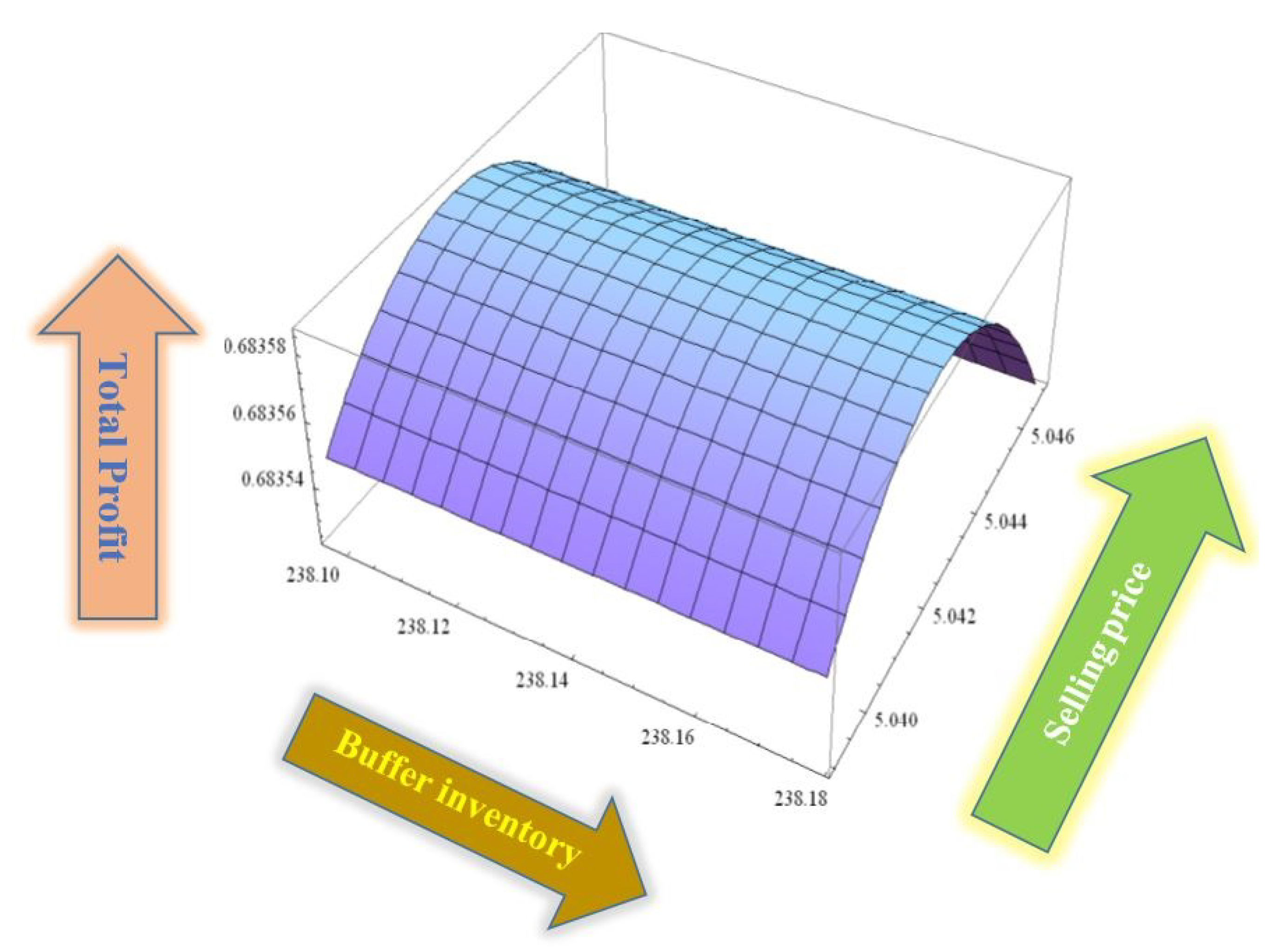
Table 4 clearly expresses that the optimality of the profit per unit item is $\$0.69$, where the per unit selling price is $\$5.04$, optimal production rate is 397 units, optimal production cost per item is $\$0.48$, optimal investment for autonomated inspection per unit is $\$11.30$, and optimal cycle length is $1.42$ days; the optimal values for $F_{nf}$ and $S_{nf}$ are $0.12$ and $0.47$ days, respectively, and the optimal buffer inventory is 238 units.

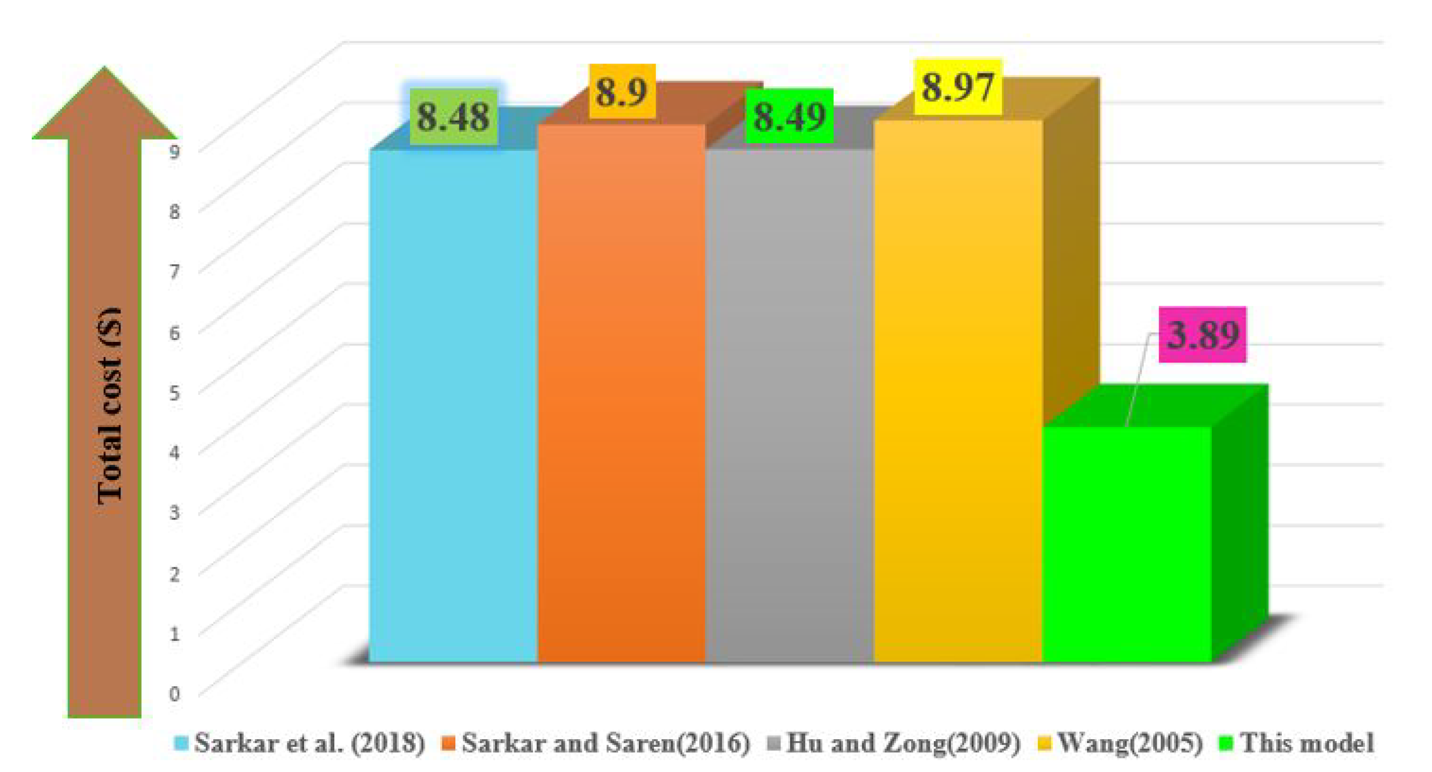
It can be observed that the cost related to this model is optimal compared to that of the existing literature, as clearly indicated in

Table 5. Total cost comparison table with existing literature.

This Model	Sarkar et al. [6]	Sarkar and Saren [5]	Hu and Zong [58]	Wang [37]
$({\mathit{T}}_{\mathit{P}\mathit{R}}^{\ast },{\mathit{F}}_{\mathit{n}\mathit{f}}^{\ast },{\mathit{S}}_{\mathit{n}\mathit{f}}^{\ast },{\mathit{M}}_{\mathit{r}\mathit{p}}^{\ast },{\mathit{\eta }}^{\ast },{\mathit{U}}_{\mathit{p}\mathit{r}}^{\ast })$	$({\mathit{T}}_{\mathit{P}\mathit{R}}^{\ast },{\mathit{F}}_{\mathit{n}\mathit{f}}^{\ast },{\mathit{S}}_{\mathit{n}\mathit{f}}^{\ast })$	$({\mathit{T}}_{\mathit{P}\mathit{R}}^{\ast },{\mathit{u}}^{\ast })$	$({\mathit{T}}_{\mathit{P}\mathit{R}}^{\ast },{\mathit{F}}_{\mathit{n}\mathit{f}}^{\ast },{\mathit{S}}_{\mathit{n}\mathit{f}}^{\ast })$	$({\mathit{T}}_{\mathit{P}\mathit{R}}^{\ast },{\mathit{u}}^{\ast })$
$\mathit{C}({\mathit{T}}_{\mathit{P}\mathit{R}}^{\ast },{\mathit{F}}_{\mathit{n}\mathit{f}}^{\ast },{\mathit{S}}_{\mathit{n}\mathit{f}}^{\ast },{\mathit{M}}_{\mathit{r}\mathit{p}}^{\ast },{\mathit{\eta }}^{\ast },{\mathit{U}}_{\mathit{p}\mathit{r}}^{\ast })$	$\mathbf{C}({\mathit{T}}_{\mathit{P}\mathit{R}}^{\ast },{\mathit{F}}_{\mathit{n}\mathit{f}}^{\ast },{\mathit{S}}_{\mathit{n}\mathit{f}}^{\ast })$	$\mathbf{C}({\mathit{T}}_{\mathit{P}\mathit{R}}^{\ast },{\mathit{u}}^{\ast })$	$\mathit{C}({\mathit{T}}_{\mathit{P}\mathit{R}}^{\ast },{\mathit{F}}_{\mathit{n}\mathit{f}}^{\ast },{\mathit{S}}_{\mathit{n}\mathit{f}}^{\ast })$	$\mathit{C}({\mathit{T}}_{\mathit{P}\mathit{R}}^{\ast },{\mathit{u}}^{\ast })$
(1.42,0.12,0.47,5.04,11.30, 397.90)	(2.04,0.058,0.251)	(1.85,0.064)	(2.05,0.062,0.239)	(1.83,0.069)
$3.89	$8.48	$8.90	$8.49	$8.97

. From Table 5, it is also clear that autonomated inspection is significantly beneficial compared to human inspection. In Sarkar and Saren’s study [5], model inspection was performed at the end of the process by humans and the cost was $\$8.90$, whereas Sarkar et al. [6] considered performing the inspection at arbitrary time intervals and the cost was $\$8.48$. Hu and Zong [58] performed an extended inspection policy without considering the inspection errors and begun the inspection in the middle of the process; the cost was $\$8.49$. Similarly, Wang [37] considered a technique wherein the inspection was performed at the end of the production without considering the inspection error; however, in his model, he considered free minimal warranty for non-inspected items and the cost for each item was $\$8.97$.

Unlike the models reported the literature, in this model, an autonomated inspection was performed at arbitrary time intervals and the total cost was $\$3.89$, which was over fifty percent less related to the other models. Furthermore, demand is considered to be dependent on the selling price and the production rate is variable. The comparison of costs of different models is graphically presented in Figure 2. Figure 2 confirms that the proposed model provides considerably improved results compared to the previously reported models. From the current study, it is clear that adaptation of autonomation strategy for inspection in an imperfect production system is really very helpful and beneficial for any production company.

Sensitivity Analysis

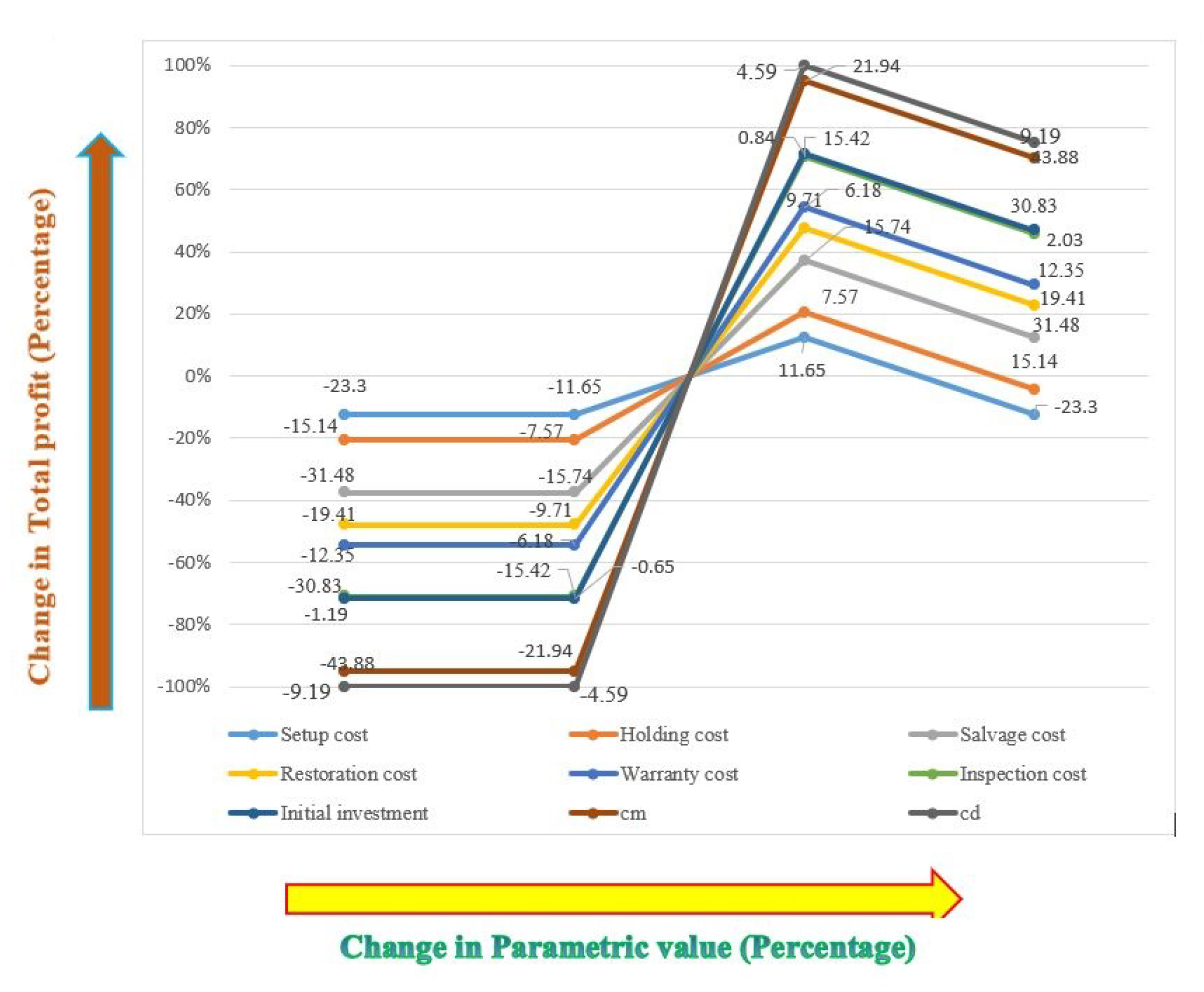
The relationship among the key parameters and total profit is extensively discussed in this section, wherein the effect of parameters such as $C_{SP}$, $C_{HP}$, $S_{cd}$, $W_{cn}$, $C_I$, $C_{RI}$, $c_d$, $c_m$, and b on the optimal solution is determined. The effect of the parameters is summarized in

Table 6. Sensitivity analysis table.

Parameters	Change (in %)	Change in TP (%)	Parameters	Change (in %)	Change in TP (%)
	50%	−23.30		50%	−15.14
	25%	−11.65		25%	−7.57
$C_{SP}$	−25%	+11.65	$C_{HP}$	−25%	+7.57
	−50%	+23.30		−50%	+15.14
	50%	−31.48		50%	−12.35
	25%	−15.74		25%	−6.18
$S_{cd}$	−25%	+15.74	$W_{cn}$	−25%	+6.18
	−50%	+31.48		−50%	+12.35
	50%	−30.83		50%	−19.41
	25%	−15.42		25%	−9.71
$C_I$	−25%	+15.42	$C_{RI}$	−25%	+9.71
	−50%	+30.83		−50%	+19.41
	50%	−1.19		50%	−9.19
	25%	−0.65		25%	−4.59
${\eta }_0$	−25%	+0.84	$c_d$	−25%	+4.59
	−50%	+2.03		−50%	+9.19
	50%	−43.88		50%	−5.77
	25%	−21.94		25%	+12.09
$c_m$	−25%	+21.94	b	−25%	+14.03
	−50%	+43.88		−50%	−

. Here, the graphical presentation in Figure 3 expresses the effect of parameters on the total profit.

Here, based on the sensitivity analysis shown in Table 6, one can make the following criticisms:

$\left(i\right)$

If setup cost $C_{SP}$ increases, the expected total profit per item $ETP(T_{PR}^{\ast },M_{rp}^{\ast },{\eta }^{\ast },U_{pr}^{\ast },F_{nf}^{\ast },S_{nf}^{\ast })$ must decrease. To increase the total profit, the system setup costs can be diminished.

$\left(ii\right)$

Table 6 reflects that the increased value of $C_{HP}$ decreases the total profit per item $ETP(T_{PR}^{\ast },M_{rp}^{\ast },{\eta }^{\ast },U_{pr}^{\ast },F_{nf}^{\ast },S_{nf}^{\ast })$. The holding cost can be diminished by reducing the run length of production $T_{PR}^{\ast }$. The reduction of the production run length will help to reduce the production and simultaneously reduce the holding cost and increase the total system profit.

$\left(iii\right)$

From Table 6, one can find that, if warranty cost, i.e., $W_{cn}$, increases, the total profit per item $ETP(T_{PR}^{\ast },M_{rp}^{\ast },{\eta }^{\ast },U_{pr}^{\ast },F_{nf}^{\ast },S_{nf}^{\ast })$ decreases. To increase the profit, the manufacturer would have to produce additional perfect items, such that less warranty cost is required, which directly helps to increase the profit of each item.

$\left(iv\right)$

Salvage cost $S_{cd}$ has a significant impact on the total profit; this can be observed from Table 6. Table 6 confirms that an increment in salvage cost results in a reduction of the total profit per item $ETP(T_{PR}^{\ast },M_{rp}^{\ast },{\eta }^{\ast },U_{pr}^{\ast },F_{nf}^{\ast },S_{nf}^{\ast })$. The incrementation of $S_{cd}$ results in an increase in the number of faulty items, which indicates the inspection of huge items, i.e., incrementation of inspection cost, causes low total profit.

$\left(v\right)$

The effect of rework cost $C_{RI}$ on total profit $ETP(T_{PR}^{\ast },M_{rp}^{\ast },{\eta }^{\ast },U_{pr}^{\ast },F_{nf}^{\ast },S_{nf}^{\ast })$ is clearly expressed in Table 6. An increased value of $C_{RI}$ implies more rework cost as well as low profit per item. Therefore, rework cost can be controlled by reducing imperfect items. Additionally, reduced production run time can reduce the total number of imperfect items and cause higher rework cost. Therefore, the production run length $T_{PR}^{\ast }$ decreases as $C_{RI}$ increases.

$\left(vi\right)$

If the system is operated at increased inspection cost $C_I$ system, then the total profit per item $ETP(T_{PR}^{\ast },M_{rp}^{\ast },{\eta }^{\ast },U_{pr}^{\ast },F_{nf}^{\ast },S_{nf}^{\ast })$ must decrease. The reduction of the inspection cost to the manufacturer must decrease the inspected fraction batch $S_{nf}^{\ast }.$ Therefore, $S_{nf}^{\ast }$ decreases as $C_I$ increases.

$\left(vii\right)$

Parameter ${\eta }_0$, i.e., the initial inspection cost for process quality and product is slightly sensitive, which is clear from Table 6. Increments in ${\eta }_0$ reduced the profit per item.

$\left(viii\right)$

The values of $c_d$ and $c_m$ are significantly sensitive toward the production costs. Increments in these parameters lead to low profit $ETP(T_{PR}^{\ast },M_{rp}^{\ast },{\eta }^{\ast },U_{pr}^{\ast },F_{nf}^{\ast },S_{nf}^{\ast })$ per item.

7. Conclusions

This research formulated an imperfect production system with the implementation of an autonomation policy to execute error-free inspection. The imperfect items were produced in an out-of-control state, and these products were identified by autonomated inspection. Furthermore, because demand is price sensitive and the production rate is variable, a more realistic result for any industrial sector can be achieved through the proposed model. The profit was optimized with the help of the optimal selling price and optimal production rate along with the optimal investment for the autonomation policy, thus making the production process smarter. To keep the brand image of the company and for customer satisfaction, salvage cost and warranty cost were incorporated for the non-inspected products. Autonomated inspection can be performed at any time interval. The numerical analysis confirmed profit optimality. This study proved that autonomated inspection can resolve TYPE-I and TYPE-II errors and maximize the total profit per item. Continuous investment for autonomation is one of the limitations of this model. One can use discrete investment instead of continuous investment for automonated (Sarkar et al. [63]) inspection policy, which may be more beneficial for some industry. One another limitation of this proposed model is the fixed setup cost, but a variable setup cost is more beneficial for some production system (Tiwari et al. [64]) and variable setup cost can be reduced by some continuous or discrete investment (Sakar and Chung [65]).

This study can be further extended by considering operational maintenance during any production process (e.g., Sana [66], Liu et al. [67]). This model can be extended by considering safety stock and random machine breakdown, as done by Sarkar et al. [54] and Ghaleb et al. [68]. The model applicability can be improved if the items are considered as defective with corrective and preventive maintenance (Sarkar et al. [69]). Considering the environmental issues, this model can be extended by considering carbon emission cost for an imperfect production model (Mishra et al. [70], Tiwari et al. [71]). To keep the environment clean, one can extend this model for green product production industry (Gao et al. [72], Pakseresht et al. [73]). This model can also be further improved by considering manufacturing and remanufacturing in the same production cycle (Saxena et al. [26]). The imperfect quality items that are considered as waste can be managed by different smart techniques (Tayyab et al. [74], Tayyab et al. [75]). This model can also be extended by considering O2O (offline and online) environment in the production industry (Pei et al. [76]).

References

- Angelopoulou, A.; Mykoniatis, K.; Boyapati, N.R. Industry 4.0: The use of simulation for human reliability assessment. Procedia Manuf. 2020, 42, 296–301. [Google Scholar] [CrossRef]
- Bueno, A.; Filho, M.G.; Castagnoli, R. Smart production planning and control in the Industry 4.0 context: A systematic literature review. Comput. Ind. Eng. 2020, 149, 106774. [Google Scholar] [CrossRef]
- Ghosh, D.; Sant, T.G.; Kuiti, M.R.; Swami, S.; Shankar, R. Strategic decisions, competition and cost-sharing contract under industry 4.0 and environmental considerations. Resour. Conserv. Recycl. 2020, 162, 105057. [Google Scholar] [CrossRef]
- Dey, B.K.; Sarkar, B.; Sarkar, M.; Pareek, S. An integrated inventory model involving discrete setup cost reduction, variable safety factor, selling price dependent demand, and investment. Rairo Oper. Res. 2019, 53, 39–57. [Google Scholar] [CrossRef] [Green Version]
- Sarkar, B.; Saren, S. Product inspection policy for an imperfect production system with inspection errors and warranty cost. Eur. J. Oper. Res. 2016, 248, 263–271. [Google Scholar] [CrossRef]
- Sarkar, B.; Sett, B.K.; Sarkar, S. Optimal production run time and inspection errors in an imperfect production system with warranty. J. Ind. Manag. Optim. 2018, 14, 267–282. [Google Scholar] [CrossRef] [Green Version]
- Sett, B.; Sarkar, S.; Sarkar, B. Optimal buffer inventory and inspection errors in an imperfect production system with regular preventive maintenance. Int. J. Adv. Manuf. Technol. 2017, 90, 545–560. [Google Scholar] [CrossRef]
- Dey, B.K.; Pareek, S.; Tayyab, M.; Sarkar, B. Autonomation policy to control work-inprocess inventory in a smart production system. Int. J. Prod. Res. 2020, in press. [Google Scholar] [CrossRef]
- Bettayeb, B.; Bassetto, S.J. Impact of type-II inspection errors on a risk exposure control approach based quality inspection plan. J. Manuf. Syst. 2016, 40, 87–95. [Google Scholar] [CrossRef]
- Hao, S.; Yang, J.; Berenguer, C. Condition-based maintenance with imperfect inspections for continuous degradation processes. Appl. Math. Model. 2020, 86, 311–334. [Google Scholar] [CrossRef]
- Shor, J.; Raz, T. Assessing the impact of human factors on data processing inspection errors. Comput. Ind. Eng. 1988, 14, 503–512. [Google Scholar] [CrossRef]
- Zhang, F.; Shen, J.; Ma, Y. Optimal maintenance policy considering imperfect repairs and non-constant probabilities of inspection errors. Reliab. Eng. Syst. Saf. 2020, 193, 106615. [Google Scholar] [CrossRef]
- Porteus, E.L. Optimal lot sizing, process quality improvement and setup cost reduction. Oper. Res. 1986, 34, 137–144. [Google Scholar] [CrossRef]
- Jamal, A.A.M.; Sarker, B.R.; Mondal, S. Optimal manufacturing batch size with rework process at a single-stage production system. Comput. Ind. Eng. 2004, 47, 77–89. [Google Scholar] [CrossRef]
- Cárdenas-Barrón, L.E. On optimal manufacturing batch size with rework process at single-stage production system. Comput. Ind. Eng. 2007, 53, 196–198. [Google Scholar] [CrossRef]
- Cárdenas-Barrón, L.E. Optimal manufacturing batch size with rework in a single-stage production system—A simple derivation. Comput. Ind. Eng. 2008, 55, 758–765. [Google Scholar] [CrossRef]
- Cárdenas-Barrón, L.E. Economic production quantity with rework process at a single-stage manufacturing system with planned backorders. Comput. Ind. Eng. 2009, 57, 1105–1113. [Google Scholar] [CrossRef]
- Sana, S.S. An economic production lot size model in an imperfect production system. Eur. J. Oper. Res. 2010, 201, 158–170. [Google Scholar] [CrossRef]
- Sana, S.S. A production-inventory model in an imperfect production process. Eur. J. Oper. Res. 2010, 200, 451–464. [Google Scholar] [CrossRef]
- Sana, S.S.; Chaudhuri, K.S. 2010. An EMQ model in an imperfect production process. Int. J. Syst. Sci. 2010, 41, 635–646. [Google Scholar] [CrossRef]
- Sana, S.S. Price-sensitive demand for perishable items–an EOQ model. Appl. Math. Comput. 2011, 217, 6248–6259. [Google Scholar] [CrossRef]
- Sarkar, B.; Moon, I. An EPQ model with inflation in an imperfect production system. Appl. Math. Comput. 2011, 217, 6159–6167. [Google Scholar] [CrossRef]
- Yoo, S.H.; Kim, D.; Park, M.S. Lot size and quality investment with quality cost analyses for imperfect production and inspection processes with commercial return. Int. J. Prod. Econ. 2012, 140, 922–933. [Google Scholar] [CrossRef]
- Sarkar, B.; Cárdenas-Barrón, L.E.; Sarkar, M.; Singgih, M.L. An economic production quantity model with random defective rate, rework process and backorders for a single-stage production system. J. Manuf. Syst. 2020, 33, 423–435. [Google Scholar] [CrossRef]
- Sarkar, B.; Dey, B.K.; Pareek, S.; Sarkar, M. A single-stage cleaner production system with random defective rate and remanufacturing. Comput. Ind. Eng. 2020, 106861. [Google Scholar] [CrossRef]
- Saxena, N.; Sarkar, B.; Singh, S.R. Selection of remanufacturing/ production cycles with an alternative market: A perspective on waste management. J. Clean. Prod. 2020, 245, 118935. [Google Scholar] [CrossRef]
- Tayyab, M.; Sarkar, B. Optimal batch quantity in a cleaner multi-stage lean production system with random defective rate. J. Clean. Prod. 2016, 139, 922–934. [Google Scholar] [CrossRef]
- Lopes, R. Integrated model of quality inspection, preventive maintenance and buffer stock in an imperfect production system. Comput. Ind. Eng. 2018, 126, 650–656. [Google Scholar] [CrossRef]
- Kim, M.S.; Kim, J.S.; Sarkar, B.; Sarkar, M.; Iqbal, M.W. An improved way to calculate imperfect items during long-run production in an integrated inventory model with backorders. J. Manuf. Syst. 2018, 47, 153–167. [Google Scholar] [CrossRef]
- Kang, C.W.; Ullah, M.; Sarkar, B.; Hussain, I.; Akhtar, R. Impact of random defective rate on lot size focusing work-in-process inventory in manufacturing system. Int. J. Prod. Res. 2017, 55, 1748–1766. [Google Scholar] [CrossRef]
- Taleizadeh, A.A.; Sarkar, B.; Hasani, M. Delayed payment policy in multi-product single-machine economic production quality model with repair failure and partial backordering. J. Ind. Manag. Optim. 2020, 16, 1273–1296. [Google Scholar] [CrossRef]
- Sarkar, M.; Sarkar, B. How does an industry reduce waste and consumed energy within a multi-stage smart sustainable biofuel production system? J. Clean. Prod. 2020, 121200. [Google Scholar] [CrossRef]
- Ullah, M.; Sarkar, B. Recovery-channel selection in a hybrid manufacturing-remanufacturing production model with RFID and product quality. Int. J. Prod. Econ. 2020, 219, 360–374. [Google Scholar] [CrossRef]
- Chryssolouris, G.; Patel, S. In Process Control for Quality Assurance. In Industrial High Technology for Manufacturing; McKee, K., Tijunelis, D., Eds.; Marcel Dekker, Inc.: New York, NY, USA, 1987; pp. 609–643. [Google Scholar]
- Salameh, M.K.; Jaber, M.Y. Economic production quantity model for items with imperfect quality. Int. J. Prod. Econ. 2000, 64, 59–64. [Google Scholar] [CrossRef]
- Wang, C.H.; Sheu, S.H. Simultaneous determination of the optimal production-inventory and product inspection policies for a deteriorating production system. Comput. Oper. Res. 2001, 28, 1093–1110. [Google Scholar] [CrossRef]
- Wang, C.H. Integrated production and product inspection policy for a deteriorating production system. Int. J. Prod. Econ. 2005, 95, 123–134. [Google Scholar] [CrossRef]
- Wang, C.H. Economic offline quality control strategy with two types inspection errors. Eur. J. Oper. Res. 2007, 179, 132–147. [Google Scholar] [CrossRef]
- Wang, C.H.; Meng, F.C. Optimal lot size and offline inspection policy. Comput. Math. Appl. 2009, 58, 1921–1929. [Google Scholar] [CrossRef] [Green Version]
- Lee, T.H. Optimal production run length and maintenance schedule for a deteriorating production system. Int. J. Adv. Manuf. Technol. 2009, 43, 959–963. [Google Scholar] [CrossRef]
- Sarkar, B. Supply chain coordination with variable backorder, inspections, and discount policy for fixed lifetime products. Math. Probl. Eng. 2016, 2016, 6318737. [Google Scholar] [CrossRef] [Green Version]
- Khanna, A.; Gautam, P.; Sarker, B.; Jaggi, C.K. Integrated vendor-buyer strategies for imperfect production systems with maintenance and warranty policy. RAIRO Oper. Res. 2020, 54, 435–450. [Google Scholar] [CrossRef] [Green Version]
- Raouf, A.; Jain, J.K.; Sathe, P.T. A cost-minimization model for multi characteristic component inspection. IIE Trans. 1983, 15, 187–194. [Google Scholar] [CrossRef]
- Duffuaa, S.O.; Khan, M. An optimal repeat inspection plan with several classifications. J. Oper. Res. Soc. 2002, 53, 1016–1026. [Google Scholar] [CrossRef]
- Khanna, A.; Kishore, A.; Sarker, B.; Jaggi, C.K. Inventory and pricing decisions for imperfect quality items with inspection errors, sales returns, and partial backorders under inflation. RAIRO Oper. Res. 2020, 54, 287–306. [Google Scholar] [CrossRef] [Green Version]
- Esmaeilian, B.; Sarkis, J.; Lewis, K.; Behdad, S. Blockchain for the future of sustainable supply chain management in Industry 4.0. Resour. Conserv. Recycl. 2020, 163, 105064. [Google Scholar] [CrossRef]
- Souza, M.L.H.; Costa, C.A.; Ramos, G.O.; Righi, R.R. A survey on decision-making based on system reliability in the context of Industry 4.0. J. Manuf. Syst. 2020, 56, 133–156. [Google Scholar] [CrossRef]
- Büchi, G.; Cugno, M.; Castagnoli, R. Smart factory performance and Industry 4.0. Technol. Forecast. Soc. Chang. 2020, 150, 119790. [Google Scholar] [CrossRef]
- Sana, S.S. Optimal selling price and lotsize with time varying deterioration and partial backlogging. Appl. Math. Comput. 2010, 217, 185–194. [Google Scholar] [CrossRef]
- Khanra, S.; Sana, S.S.; Chudhuri, K. An EOQ model for perishable item with stock and price dependent demand rate. Int. J. Math. Oper. Res. 2010, 2, 320–335. [Google Scholar] [CrossRef]
- Taleizadeh, A.A.; Kalantari, S.S.; Cárdenas-Barrón, L.E. Pricing and lot sizing for an EPQ inventory model with rework and multiple shipments. TOP 2016, 24, 143–155. [Google Scholar] [CrossRef]
- Pal, B.; Sana, S.S.; Chudhuri, K. Multi-item EOQ model while demand is sales price and price break sensitive. Appl. Math. Comput. 2012, 29, 2283–2288. [Google Scholar] [CrossRef]
- Khouja, M.; Mehrez, A. Economic production lot size model with variable production rate and imperfect quality. J. Oper. Res. Soc. 1994, 4, 1405–1417. [Google Scholar] [CrossRef]
- Sarkar, B.; Sana, S.S.; Chaudhuri, K.S. An imperfect production process for time varying demand with inflation and time value of money—An EMQ model. Expert Syst. Appl. 2011, 38, 13543–13548. [Google Scholar] [CrossRef]
- Sarkar, B.; Majumder, A.; Sarkar, M.; Kim, N.; Ullah, M. Effects of variable production rate on quality of products in a single-vendor multi-buyer supply chain management. Int. J. Adv. Manuf. Technol. 2018, 99, 567–581. [Google Scholar] [CrossRef]
- Majumder, A.; Jaggi, C.K.; Sarkar, B. A multi-retailer supply chain model with backorder and variable production cost. RAIRO Oper. Res. 2018, 52, 943–954. [Google Scholar] [CrossRef]
- Dey, B.K.; Sarkar, B.; Pareek, S. A two-echelon supply chain management with setup time and cost reduction, quality improvement and variable production rate. Mathematics 2019, 7, 328. [Google Scholar] [CrossRef] [Green Version]
- Hu, F.; Zong, Q. Optimal production run time for a deteriorating production system under an extended inspection policy. Eur. J. Oper. Res. 2009, 196, 979–986. [Google Scholar] [CrossRef]
- Sun, Z.; Hupman, A.C.; Abbas, A.E. The value of information for price dependent demand. Eur. J. Oper. Res. 2021, 288, 511–522. [Google Scholar] [CrossRef]
- Chen, C.K.; Lo, C.C.; Weng, T.C. Optimal production run length and warranty period for an imperfect production system under selling price dependent on warranty period. Eur. J. Oper. Res. 2017, 259, 401–412. [Google Scholar] [CrossRef]
- Paul, S.K.; Sarker, R.; Essam, D. Managing disruption in an imperfect production–inventory system. Comput. Ind. Eng. 2015, 84, 101–112. [Google Scholar] [CrossRef]
- Lin, Y.H.; Chen, J.M.; Chen, Y.C. The impact of inspection errors, imperfect maintenance and minimal repairs on an imperfect production system. Math. Comput. Model. 2011, 53, 1680–1691. [Google Scholar] [CrossRef]
- Sarkar, M.; Pan, L.; Dey, B.K.; Sarkar, B. Does the autonomation policy really help in a smart production system for controlling defective production? Mathematics 2020, 8, 1142. [Google Scholar] [CrossRef]
- Tiwari, S.; Kazemi, N.; Modak, N.M.; Cárdenas-Barrón, L.E.; Sarkar, S. The effect of human errors on an integrated stochastic supply chain model with setup cost reduction and backorder price discount. Int. J. Prod. Econ. 2020, 226, 107643. [Google Scholar] [CrossRef]
- Sarkar, M.; Chung, B.D. Flexible work-in-process production system in supply chain management under quality improvement. Int. J. Prod. Res. 2020, 58, 3821–3838. [Google Scholar] [CrossRef]
- Sana, S. Preventive maintenance and optimal buffer inventory for products sold with warranty in an imperfect production system. Int. J. Prod. Res. 2012, 50, 6763–6774. [Google Scholar] [CrossRef]
- Liu, Q.; Dong, M.; Chem, F.; Liu, W.; Ye, C. Multi-objective imperfect maintenance optimization for production system with an intermediate buffer. J. Manuf. Syst. 2020, 56, 452–462. [Google Scholar] [CrossRef]
- Ghaleb, M.; Zolfagharinia, H.; Taghipour, S. Real-time production scheduling in the Industry-4.0 context: Addressing uncertainties in job arrivals and machine breakdowns. Comput. Oper. Res. 2020, 123, 105031. [Google Scholar] [CrossRef]
- Sarkar, B.; Sana, S.S.; Chaudhuri, K.S. An Economic production quantity model with stochastic demand in an imperfect production system. Int. J. Serv. Oper. Manag. 2011, 9, 259–283. [Google Scholar] [CrossRef]
- Mishra, U.; Wu, J.Z.; Sarkar, B. A sustainable production-inventory model for a controllable carbon emissions rate under shortages. J. Clean. Prod. 2020, 256, 120268. [Google Scholar] [CrossRef]
- Tiwari, S.; Ahmed, W.; Sarkar, B. Sustainable ordering policies for non-instantaneous deteriorating items under carbon emission and multi-trade-credit-policies. J. Clean. Prod. 2019, 240, 118–183. [Google Scholar] [CrossRef]
- Gao, J.; Xiao, Z.; Wei, H.; Zhou, G. Dual-channel green supply chain management with eco-label policy: A perspective of two types of green products. Comput. Ind. Eng. 2020, 146, 106613. [Google Scholar] [CrossRef]
- Pakseresht, M.; Shirazi, B.; Mahdavi, I.; Mahdavi-Amiri, N. Toward sustainable optimization with stackelberg game between green product family and downstream supply chain. Sustain. Prod. Consum. 2020, 23, 198–211. [Google Scholar] [CrossRef]
- Sarkar, B.; Tayyab, M.; Kim, N.; Habib, M.S. Optimal production delivery policies for supplier and manufacturer in a constrained closed-loop supply chain for returnable transport packaging through metaheuristic approach. Comput. Ind. Eng. 2019, 135, 987–1003. [Google Scholar] [CrossRef]
- Tayyab, M.; Jemai, J.; Han, L.; Sarkar, B. A sustainable development framework for a cleaner multi-item multi-stage textile production system with a process improvement initiative. J. Clean. Prod. 2020, 246, 119055. [Google Scholar] [CrossRef]
- Pei, Z.; Wooldridge, B.R.; Swimberghe, K.R. Manufacturer rebate and channel coordination in O2O retailing. J. Retail. Consum. Serv. 2021, 58, 102268. [Google Scholar] [CrossRef]
Figure 1.
Graphical representation of total profit with respect to buffer inventory and selling price.
Figure 2.
Graphical representation of cost for different existing literature.
Figure 3.
Effect of parametric values on expected total profit .