The Diagnosability of Wheel Networks with Missing Edges under the Comparison Model

Abstract

The diagnosability is an essential subject for the reliability of a multiple CPU system. As a celebrated topology structure of interconnection networks, an n-dimensional wheel network $C{W}_n$ has numerous great features. In this paper, we discuss the diagnosability of $C{W}_n$ with missing edges under the comparison model. Both the local diagnosability and the strong local diagnosability feature are studied; this feature depicts the equivalence of the local diagnosability of a node and its degree. We demonstrate that $C{W}_n(n\ge 6)$ possesses this feature, containing the strong feature even with up to $2n-4$ missing edges in it, and the outcome is ideal regarding the amount of missing edges.

1. Introduction

Numerous multiple CPU systems have interconnection networks (networks for short) as fundamental topologies, and a network is normally spoken to by a graph where nodes speak to CPUs and links speak to communication links between CPUs. For a system, a few CPUs may fizzle in the system, so CPU flaw distinguishing proof assumes a significant job for solid figuring. The distinguishing process is known as the diagnosis of the system. A system is supposed to be t-diagnosable if all broken CPUs can be distinguished without substitution, given that the quantity of faults presented does not surpass t. The diagnosability $t\left(G\right)$ of a system G is the largest amount of t such that G is t-diagnosable [1,2,3].

A few diagnosis models (e.g., PMC model [4], BGM model [5] and MM model [6]) are suggested to examine the ability to be diagnosed. Under the PMC model [4], the diagnosis of a system G is achieved through two adjacent nodes in G testing each other. The BGM model [5] uses the same testing strategy as the PMC model, but it assumes that a faulty unit is always tested as faulty regardless of the state of the tester. Specifically, the MM model, is notable and broadly utilized. In the MM model, likewise named the comparison model, to diagnose a system, a node sends the similar assignment to two of its neighbors, and afterward looks at their responses. Sengupta and Dahbura [1] suggested an uncommon instance of the MM model, named the MM${}^{*}$ model, in which every node can test its any couple of adjacent nodes. These were investigated within the PMC model and MM model or MM${}^{*}$ model. Fan [2] studied the diagnosability of crossed cubes under the comparison diagnosis model. Lai et al. [3] discussed the conditional diagnosability measures for large multiprocessor systems under the PMC model. Chang et al. [7] studied the structural properties and conditional diagnosability of star graphs by using the PMC model. Feng et al. [8] gave the nature diagnosability of wheel graph networks under the PMC model and MM${}^{*}$ model. Lin et al. [9] investigated the conditional diagnosability of Cayley graphs generated by transposition trees under the comparison diagnosis model. Peng et al. [10] gave the g-good-neighbor conditional diagnosability of hypercube under PMC model. Wang et al. [11] studied the 1-good-neighbor diagnosability of Cayley graphs generated by transposition trees under the PMC model and MM${}^{*}$ model. Wang et al. [12] gave the 1-good-neighbor connectivity and diagnosability of Cayley graphs generated by complete graphs under the PMC model and MM${}^{*}$ model. Yuan et al. [13] obtained the g-good-neighbor conditional diagnosability of k-ary n-cubes under the PMC model and MM${}^{*}$ model.

Hsu and Tan [14] observed that in case we only consider the global faulty or fault-free status in a t-diagnosable system, at that point we lose some local subtleties of the system. Therefore, Hsu and Tan [14] suggested a measure of the ability to be diagnosed for a multiple CPU system G, which is the local diagnosability of G. This measure considers the local diagnosability of each CPU rather than the entire system. Chiang and Tan [15] suggested a helpful local structure named an extended star to ensure the node diagnosability and a sufficient condition to decide the local diagnosability under the MM model. They found that there is a solid connection between the local diagnosability of G and the classical diagnosability of G. The system G has the strong local diagnosability feature (property) if the local diagnosability of each node is equivalent to its degree in G. Following this idea, the strong local diagnosability has been generally investigated. Chiang et al. [16] found that an n-dimensional star has the strong local diagnosability even with up to $n-3$ missing edges. Furthermore, Cheng et al. [17] obtained the strong local diagnosability to $(n,k)$-star graphs and the Cayley Graphs produced by 2-trees. In 2018, Wang and Ma [18] demonstrated that an n-alternating group graph possesses the strong local diagnosability feature even with up to $2n-7$ missing edges in it under the MM${}^{*}$ model. Wang et al. [19] showed that an n-dimensional bubble-sort star graph $B{S}_n(n\ge 5)$ has the feature even with up to $2n-5$ missing edges, under the MM${}^{*}$ model. Here, we present that an n-dimensional wheel network $C{W}_n(n\ge 6)$ has the local diagnosability feature even with up to $2n-4$ missing edges in it under the MM${}^{*}$ model, and the consequence is optimal respect to the number of missing edges.

2. Preliminaries

2.1. Definitions and Presentations

A multiple CPU system is presented as a directionless graph $G=(V,E)$, whose vertices (nodes) determine CPUs and edges (links) determine communication links. Given a nonempty node subset $V^{\prime }$ of V, the induced subgraph by $V^{\prime }$ in G, denoted by $G\left[V^{\prime }\right]$, is a graph, whose node set is $V^{\prime }$ and the link set is the set of each link of G with both endpoints in $V^{\prime }$. The degree $d_G\left(v\right)$ of a node v is the amount of links incident with v. We denote by $\delta \left(G\right)$ the minimum degrees of nodes of G. We describe the neighborhood $N_G\left(v\right)$ of a node v in G as set of nodes adjacent to v. u is named a neighbor or a neighbor node of v for $u\in N_G\left(v\right)$. Let $S\subseteq V$. We use $N_G\left(S\right)$ to represent the set ${\cup }_{v\in S}{N}_G\left(v\right)\backslash S$. For neighborhoods and degrees, we shall typically neglect the subscript for the graph once no misperception ascends. A graph G is k-regular if for all $v\in V$, $d_G\left(v\right)=k$. The connectivity $\kappa \left(G\right)$ of a connected graph G is the minimum number of nodes whose exclusion effects in a disconnected graph or just a node left when G is complete. The edge-connectivity $\lambda \left(G\right)$ of G is the minimum number of links whose exclusion outcomes in a disconnected graph. A graph is bipartite if its node set can be partitioned into two subsets X and Y its fragments such that $G\left[X\right]$ and $G\left[Y\right]$ has no link. The girth is the length of the shortest cycle in a graph G. The automorphism group of a graph G is transitive if there is an automorphism $\phi$ to arbitrary couples $u,v$ of nodes in G such that $\phi \left(u\right)=v$. Here, G is named node transitive. For graph-related vocabulary and representation not described we refer the reader to [20].

Proposition 1

([20]). For a graph $G=(V,E)$, $\kappa \left(G\right)\le \lambda \left(G\right)\le \delta \left(G\right)$.

2.2. The MM${}^{*}$ Model

The MM model is originally suggested by Malek and Maeng in [6]. In the MM model, the diagnosis is performed by transmitting the same testing errand to a couple of CPUs and looking at their responses. Within the MM model, we generally accept the yield of a comparison achieved by a defective CPU is questionable. The comparison scheme of a system $G=(V,E)$ is presented as a multi-graph, denoted by $M=\left(V\right(G),L)$, where L is the labeled-link set. A labeled link ${(u,v)}_w\in L$ determines an evaluation where two vertices u and v are compared by a node w, which indicates $uw,vw\in E\left(G\right)$. The collection of each comparison outcome in $M=\left(V\right(G),L)$ is named the syndrome of the diagnosis, denoted by $\sigma$. If the comparison ${(u,v)}_w$ differs, then $\sigma \left({(u,v)}_w\right)=1$, else, $\sigma \left({(u,v)}_w\right)=0$. Thereat, a syndrome is a mapping from L to $\{0,1\}$. Sengupta and Dahbura [21] suggested MM${}^{*}$ model. The MM${}^{*}$ model is a specific type of the MM model. Within the MM${}^{*}$ model, each comparison of G is in the comparison system of G, i.e., if $uw,vw\in E\left(G\right)$, then ${(u,v)}_w\in L$. The set of each defective CPU in the system is named a faulty set. It can be an arbitrary subset of $V\left(G\right)$. For a given a syndrome $\sigma$. Then a subset of nodes $F\subseteq V\left(G\right)$ is supposed to be consistent with $\sigma$ if $\sigma$ can be formed from the state, for all ${(u,v)}_w\in L$ such that $w\in V\backslash F$, $\sigma \left({(u,v)}_w\right)=1$ if and only if at least one of $\{u,v\}$ is in F. Let $\sigma \left(F\right)$ signify the set of each syndrome that F is consistent with. Let $F_1$ and $F_2$ be two different sets in $V\left(G\right)$. If $\sigma \left(F_1\right)\cap \sigma \left(F_2\right)=\varnothing$, it is said $F_1$ and $F_2$ be a distinguishable pair (couple); else, $(F_1,F_2)$ is an indistinguishable pair (couple).

The primary merit of the MM model is its simplicity in identifying a faulty CPU because the comparison of pairs of CPUs seems to be easier than testing one CPU by another or others [22]. The MM model has two advantages in fault identification: the MM model requires no additional hardware; transient and permanent faults may be identified before the comparison program has completed [22]. Sengupta et al. [21] investigated many significant features of a diagnosable system using the MM model. The MM${}^{*}$ model might result in the development of a polynomial-time diagnosis algorithm in general MM self-diagnosable systems, and complexity leads to determining the diagnosability level of systems [23].

2.3. Wheel Networks

The wheel networks [24] are a famous topology construction in interconnection networks. We consider this topology in this section.

Let Q be a finite group, and assume S be a spanning set of Q such that S does not contain the identity element. The directed Cayley graph $Cay(S,Q)$ is described as follows: its node set is Q, its arc set is $\left\{\right(g,gs):g\in Q,s\in S\}$. If for each $s\in S$, $s^{-1}\in S$, then all of arc sets of $Cay(S,Q)$ have parallel links going in diverse directions. If we replace two arcs of the parallel link going in different directions in $Cay(S,Q)$ with a link, then we get a directionless graph named the undirected Cayley graph. Each Cayley graph in this paper is an undirected Cayley graph.

In the permutation $\left(\genfrac{}{}{0pt}{}{12\cdots n}{p_1{p}_2\cdots p_n}\right)$, $i⟶p_i$. For convenience, we signify the permutation $\left(\genfrac{}{}{0pt}{}{12\cdots n}{p_1{p}_2\cdots p_n}\right)$ by $p_1{p}_2\cdots p_n$. Each permutation is denoted by a product of cycles [25]. For instance, $\left(\genfrac{}{}{0pt}{}{123}{312}\right)=\left(132\right)$. Specially, $\left(\genfrac{}{}{0pt}{}{12\cdots n}{12\cdots n}\right)=\left(1\right)$. The product $\sigma \tau$ of two permutations is the composition function $\tau$ trailed by $\sigma$, i.e., $\left(12\right)\left(13\right)=\left(132\right)$. For algebraic terminology and notation not described here we refer to [25].

Let $\left[n\right]=\{1,2,\cdots ,n\}$, and consider H as a simple connected graph whose node set is $\left[n\right](n\ge 3)$. Each link of H is reflected as the transposition in symmetric group $S_n$, and so the link set of H corresponds to a transposition set S in $S_n$. Therefore, H is named a transposition simple graph. The Cayley graph Cay$(S,\langle S\rangle )$, denoted by Cay$(H,\langle S\rangle )$, is named the corresponding Cayley graph of H. As mentioned in [26], $\langle S\rangle =S_n$. Once H is a tree (resp. path, star) of n nodes, the corresponding Cayley graph is named an n-dimensional transposition tree (resp. bubble-sort graph, star graph), and denoted by $C{\Gamma }_n$ (resp. $B_n$, $S_n$) [26].

Proposition 2

([27]). $B{S}_n$ is $(2n-3)$-regular for $n\ge 4$.

Proposition 3

([28]). $\kappa \left(B{S}_n\right)=2n-3$ for $n\ge 4$.

Once H is a sector $S{E}_n$ of $n(n\ge 3)$ nodes, i.e., $V\left(S{E}_n\right)=\left[n\right]$ and $E\left(S{E}_n\right)=\{(1,k):2\le k\le n\}\cup \{(k,k+1):2\le k\le n-1\}$, the corresponding Cayley graph $Cay(S{E}_n,S_n)$ is named an n-dimensional bubble-sort star graph [27], denoted by $B{S}_n$. Once H is a wheel $W_n$ of $n(n\ge 4)$ nodes, i.e., $V\left(W_n\right)=\left[n\right]$ and $E\left(W_n\right)=\{(1,k):2\le k\le n\}\cup \{(k,k+1):2\le k\le n-1\}\cup \left\{(2,n)\right\}$, the corresponding Cayley graph $Cay(W_n,S_n)$ is named an n-dimensional wheel network [24], denoted by $C{W}_n$. In fact, an n-dimensional wheel network $C{W}_n$ is the graph with node set $V\left(C{W}_n\right)$ = $S_n$ in which 2 nodes u, v are adjacent if and only if $u=v(1,k)$, $2\le k\le n$, or $u=v(k,k+1)$, $2\le k\le n-1$, or $u=v(2,n)$.

As can be seen in [27,29], the bubble-sort star graph $B{S}_n$ possesses lesser diameter than $B_n$, equal diameter to $S_n$, and larger connectivity than $B_n$ and $S_n$, and the ability to be embedded of the bubble-sort star graph is far superior to that of the star graph. Consequently, $B{S}_n$ utilizes the benefits of $S_n$ and $B_n$, and overcomes their own limitations. Note that the diameters of $B{S}_n$ and $C{W}_n$ are both equal to $\lfloor \frac{3(n-1)}{2}\rfloor$ for $n\ge 7$ [27,30], and the $B{S}_n$ can be embedded into a $C{W}_n$, $C{W}_n$ outperforms $B{S}_n$ in connectivity [8,28]. Consequently, the wheel network is the popular and multipurpose net system for multiple CPU systems.

Notice that $C{W}_n$ is a special Cayley graph. This graph possesses some features.

Proposition 4

([31]). For each integer $n\ge 4$, $C{W}_n$ is $(2n-2)$-regular and node transitive.

Proposition 5

([31]). For each integer $n\ge 4$, $C{W}_n$ is bipartite.

Proposition 6

([8]). For each integer $n\ge 4$, the girth of $C{W}_n$ is 4.

$C{W}_n$ can be partitioned into n disjoint subgraphs $C{W}_n^1,C{W}_n^2,\cdots ,C{W}_n^n$, where each node $u=u_1{u}_2\cdots u_n\in V\left(C{W}_n^i\right)$ takes a fixed integer i in the last place $u_n$ for $i\in \left[n\right]$. Obviously, $C{W}_n^i$ is isomorphic to $B{S}_{n-1}$, where $B{S}_{n-1}$ is an $(n-1)$-dimensional bubble-sort star graph. Let $v\in V\left(C{W}_n\right)$, then $v\left(1n\right),v\left(2n\right)$ and $v(n-1,n)$ are named outside neighbors of v. A link is named a cross-edge concerning the given factorization if its two nodes are in different $C{W}_n^i$’s.

3. The Local Diagnosability

Let $F_1$ and $F_2$ be two different subsets of V for a system $G=(V,E)$, and let the symmetric difference $F_1\Delta F_2=(F_1\backslash F_2)\cup (F_2\backslash F_1)$.

Definition 1

([4]). A system G is t-diagnosable if all the faulty processors can be precisely pointed out given that the number of faulty processors is at most t.

Lemma 1

([21]). A system $G=(V,E)$ is t-diagnosable if and only if, for every couple of different set of nodes $(F_1,F_2)$ with $|F_1|\le t$ and $|F_2|\le t$, $(F_1,F_2)$ is a distinguishable pair.

Lemma 2

([21]). Let $F_1$ and $F_2$ be two different subsets of nodes. $(F_1,F_2)$ is a distinguishable couple if and only if at least one of the next situations is fulfilled:

(1) 

$\exists u,w\in V\backslash F_1\backslash F_2$ and $\exists v\in (F_1\backslash F_2)\cup (F_2\backslash F_1)$ such that ${(u,v)}_w\in L$.

(2) 

$\exists u,v\in F_1\backslash F_2$ and $\exists w\in (V\backslash F_1\backslash F_2)$ such that ${(u,v)}_w\in L$, or

(3) 

$\exists u,v\in F_2\backslash F_1$ and $\exists w\in (V\backslash F_1\backslash F_2)$ such that ${(u,v)}_w\in L$.

Opposite to the global sense in system diagnosis, Chiang and Tan [15] determined a local idea, named the local diagnosability of an assumed node in a system. This technique needs only the precise identification of the defective or defective-free position of a single node. The concept of local diagnosability is presented.

Definition 2

([14]). A system $G=(V,E)$ is locally t-diagnosable at a node x if, assumed a test syndrome ${\sigma }_F$ given by the system within the presence of a set of faulty vertices F comprising of x with $\left|F\right|\le t$, each set of faulty nodes $F^{\prime }$ is consistent with ${\sigma }_F$ and $|F^{\prime }|\le t$, must also contain node x.

An equivalent method of declaring the overhead description is specified here.

Definition 3

([14]). A system $G=(V,E)$ is locally t-diagnosable at a node x for every different couple of faulty subsets $F_1$ and $F_2$ of V with $|F_1|\le t$ and $|F_2|\le t$ if $x\in F_1\Delta F_2$, and $F_1$ and $F_2$ is distinguishable.

The local diagnosability of an assumed node in given here:

Definition 4

([14]). The local diagnosability $t_l\left(x\right)$ of a node x in a system $G=(V,E)$ is described as the maximum number of t for G that is locally t-diagnosable at x, i.e., $t_l\left(x\right)=max\{t:$G$islocally$t$-diagnosableatx\}$.

The notion of a system that is t-diagnosable at a node is consistent with the classical notion of a system that is t-diagnosable in a global sense. The connection between those two is as follows:

Lemma 3

([14]). A system $G=(V,E)$ is t-diagnosable if and only if G is locally t-diagnosable at each node of G.

Lemma 4

([14]). The diagnosability $t\left(G\right)$ of a system $G=(V,E)$ is equivalent to the minimum value within the local diagnosability of each node in G, i.e., $t\left(G\right)=min\{t_l\left(x\right):\forall x\in V\left(G\right)\}$.

From Lemma 4, we can identify the diagnosability of a system by figuring the local diagnosability of every node. The diagnosability of many famous networks which are node-symmetric can be identified using the effective measure. To assure the local diagnosability of a node x, an extended star structure at the node x is suggested as given next:

Definition 5

([15]). Fix a node x in a graph $G=(V,E)$ and a positive integer $p\le d_G\left(x\right)$. An extended star $ES(x;p)$ in x of degree p is a subgraph of G with the node set $V\left(ES(x;p)\right)=\left\{x\right\}\cup \{v_{ij}:i=1,2,\cdots ,p;j=1,2,3,4\}$, and the link set $E\left(ES(x;p)\right)=\{(x,v_{k1}),(v_{k1},v_{k2}),(v_{k2},v_{k3}),(v_{k3},v_{k4}):k=1,2,\cdots ,p\}$.

Here, x is named the root of $ES(x;p)$. An extended star is an important structure in figuring the local diagnosability of a given node. The time complexity of the algorithm to diagnose a given CPU is bounded by $O\left(logN\right)$ and that to diagnose all the faulty CPUs in a system with N CPUs is bounded $O\left(NlogN\right)$ under the comparison model, provided there is an extended star structure at each CPU and that the time for looking up the testing result of a comparator in the syndrome table is constant, where N is the total number of CPUs [15].

Lemma 5

([15]). Let x be a node in a graph $G=(V,E)$ with $d_G\left(x\right)=p$. The local diagnosability of x is p if there is an extended star $ES(x;p)$ in G at x.

Notice that the local diagnosability $t_l\left(x\right)$ of a node x may or may not be equal to its degree. So two concepts are suggested as follows:

Definition 6

([14]). Let x be a node within a graph $G=(V,E)$. The node x has the strong local diagnosability feature if the local diagnosability of x is equivalent to its degree in G, i.e., $t_l\left(x\right)=d_G\left(x\right)$.

Definition 7

([14]). Let $G=(V,E)$ be a graph. G contains the strong local diagnosability feature if each node in G possesses the strong local diagnosability feature.

The diagnosability of a system may be derived straightforwardly.

4. The Diagnosability of Wheel Networks

Lemma 6

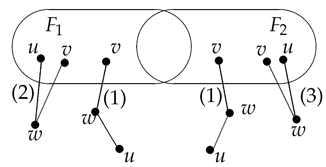
([21]). Under the MM* model, a system $G=(V,E)$ is t-diagnosable at a node x if and only if for all different couples of faulty subsets $F_1$ and $F_2$ of V with $|F_1|\le t$ and $|F_2|\le t$, and $x\in F_1\Delta F_2$, $(F_1,F_2)$ satisfies one of the next conditions:

(1)

There exist two nodes $u,w\in V\left(G\right)\backslash (F_1\cup F_2)$ and 1 node $v\in F_1\Delta F_2$ such that $uw\in E\left(G\right)$ and $vw\in E\left(G\right)$;

(2)

There exist two nodes $u,v\in F_1\backslash F_2$ and there exists 1 node $w\in V\left(G\right)\backslash (F_1\cup F_2)$ such that $uw\in E\left(G\right)$ and $vw\in E\left(G\right)$;

(3)

There exist two nodes $u,v\in F_2\backslash F_1$ and there exists a node $w\in V\left(G\right)\backslash (F_1\cup F_2)$ such that $uw\in E\left(G\right)$ and $vw\in E\left(G\right)$ (see Figure 1).

Lemma 7

([19]). For every node x in the bubble-sort graph $B{S}_n$ with $n\ge 5$, there is an extended star $ES(x;2n-3)$ in $B{S}_n$ at x.

Lemma 8.

For every node x in the wheel network $C{W}_n$ with $n\ge 6$, there is an extended star $ES(x;2n-2)$ in $C{W}_n$ at x.

Proof. 

We may partition $C{W}_n$ into n disjoint subgraphs $C{W}_n^1,C{W}_n^2,\cdots ,C{W}_n^n$, where each node $u=u_1{u}_2\cdots u_n\in V\left(C{W}_n^i\right)$ possesses a fixed integer i in the last position $u_n$ for $i\in \left[n\right]$. Obviously, $C{W}_n^i$ is isomorphic to $B{S}_{n-1}$, where $B{S}_{n-1}$ is an $(n-1)$-dimensional bubble-sort star graph.

We will determine an extended star $ES(x;2n-2)$ as a subgraph of $C{W}_n$ at a given node x. By Proposition 4, $C{W}_n$ is node transitive. Therefore, $\left(1\right)\in V\left(C{W}_n^n\right)$ can be chosen as the root of $ES(x;2n-2)$, i.e., $x=\left(1\right)$, where $\left(1\right)$ is the identity element of the symmetric group $S_n$. By Lemma 7, for the bubble-sort graph $B{S}_n$ with $n\ge 5$, there is an extended star $ES(x;2n-3)$ in $B{S}_n$ at x. So there is an extended star $ES(x;2(n-1)-3)$ in $C{W}_n^n$ at x. Note that$\left(1\right)$ has three outside neighbor nodes $\left(1n\right),\left(2n\right)$ and $(n-1,n)$, where $\left(1n\right)\in V\left(C{W}_n^1\right),\left(2n\right)\in V\left(C{W}_n^2\right)$ and $(n-1,n)\in V\left(C{W}_n^{n-1}\right)$. Notice that the 3-path $P_1=\langle \left(1n\right),\left(12n\right),\left(132n\right),\left(13n\right)\rangle$ is in $C{W}_n^1$, and the 3-path $P_2=\langle \left(2n\right),\left(1n2\right),\left(13n2\right),\left(23n\right)\rangle$ is in $C{W}_n^2$, and the 3-path $P_3=\langle (n-1,n),(n-1,n)\left(12\right),(n-1,n)\left(13\right),(n-1,n)\left(23\right)\rangle$ is in $C{W}_n^{n-1}$. We connected $P_1,P_2$ and $P_3$ to x, and then combine them with $ES(x;2n-5)$. Thus, we can obtain an extended star $ES(x;2n-2)$ in $C{W}_n$ at $\left(1\right)$, i.e., an extended star $ES(x;2n-2)$ exists in $C{W}_n$ at x. □

Theorem 1.

Let $C{W}_n$ be an n-dimensional wheel network with $n\ge 6$. Then the diagnosability of $C{W}_n$ is $2n-2$, i.e., $t\left(C{W}_n\right)=2n-2$ and $C{W}_n$ possesses the strong local diagnosability feature.

Proof. 

By Lemmas 5 and 8, the local diagnosability of every node x of $C{W}_n$ is $2n-2$. By Lemma 4, the diagnosability of $C{W}_n$ is $2n-2$, i.e., $t\left(C{W}_n\right)=2n-2$. Since the degree of every node x of $C{W}_n$ is $2n-2$, the local diagnosability of every node is equivalent to its degree in $C{W}_n$. By Lemma 7, $C{W}_n$ has the strong local diagnosability feature. □

Sometimes, many links in a multiple CPU system may be missing. A missing edge implies that a link between 2 CPUs that was faulty. The existence of missing edges in a system may affect the diagnosability of the whole system, and degrees and the local diagnosability of some nodes. Especially, in a regular graph, nodes that are adjacent to missing edges have lower degrees than others. Hence, those nodes may not keep the strong local diagnosability feature, and the graph may not keep the strong local diagnosability feature again. Those new degrees can be used to determine whether the incomplete graph keeps the strong local diagnosability feature or not. Next, we demonstrate that an n-dimensional wheel network $C{W}_n(n\ge 6)$ keeps the strong local diagnosability feature even with up to $2n-4$ missing edges.

Lemma 9

([19]). Let $B{S}_n$ be the bubble-sort graph with $n\ge 5$, and let $F_e$ be an arbitrary set of missing edges with $|F_e|\le 2n-5$. Thus $B{S}_n-F_e$ possesses the strong local diagnosability feature for every node x in $B{S}_n$ with missing edges $F_e$, and outcome is ideal, respectful to the number of missing edges.

Lemma 10.

Let $F_e$ be an arbitrary set of missing edges with $|F_e|\le 2n-4$. For every node x in $C{W}_n(n\ge 6)$, there is an extended star $ES(x;d_{C{W}_n-F_e}\left(x\right))$ at x.

Proof. 

By Proposition 4, $C{W}_n$ is node transitive. Therefore, $\left(1\right)$ can be chosen as the root of an extended star $ES(x;d_{C{W}_n-F_e}\left(x\right))$, i.e., $x=\left(1\right)$, where $\left(1\right)$ is the identity element of the symmetric group $S_n$. $C{W}_n$ can be partitioned into n disjoint subgraphs $C{W}_n^1,C{W}_n^2,\cdots ,C{W}_n^n$, where each node $u=u_1{u}_2\cdots u_n\in V\left(C{W}_n^i\right)$ has a fixed integer i in the last position $u_n$ for $i\in \left[n\right]$. Clearly, $C{W}_n^i$ is isomorphic to $B{S}_{n-1}$, where $B{S}_{n-1}$ is the bubble-sort star graph with the dimension $n-1$.

Let $F_e^i=F_e\cap E\left(C{W}_n^i\right)$ for $1\le i\le n$, and $F^{*}=F_e\cap (E\left(C{W}_n\right)\backslash {\sum }_{i=1}^{n}E\left(C{W}_n^i\right))$, then $F_e=F^{*}\cup F_e^1\cup \cdots \cup F_e^n$. For convenience, let $\tilde{F}=F^{*}\cap \{xu,xv,xw\}$, and denote $u=\left(1n\right)$, $v=\left(2n\right)$ and $w=(n-1,n)$ three outside neighbors of $\left(1\right)$. To prove this lemma, we need to discuss whether $\tilde{F}$ is an empty set or not. When $\tilde{F}=\varnothing$, the first step is to discover an extended star $ES(x;d_{C{W}_n^n-F_e^n}\left(x\right))$ in $C{W}_n^n-F_e^n$; the second step is to find a 3-path $P_u$ in $C{W}_n^1$, a 3-path $P_v$ in $C{W}_n^2$ and a 3-path $P_w$ in $C{W}_n^{n-1}$; the third step is to connect $P_u$, $P_v$ and $P_w$ to x. Then, an extended star $ES(x;d_{C{W}_n-F_e}\left(x\right))$ is found in $C{W}_n-F_e$ at x, (with $ES(x;d_{C{W}_n-F_e}\left(x\right))$ written simply as B). For the case of $\tilde{F}\ne \varnothing$, we obtain an extended star to satisfy the lemma by removing any 4-path that contains any link of $\tilde{F}$ and starts at x from B.

It should be noted that removing a 4-path P from a graph G means removing all nodes and links of the 4-path except y from a graph G in this paper, where y is the only common node of P and G.

Firstly, we give two claims as follows.

Claim 1.

If $|F_e^i|\le 2n-7$, then there exists an extended star $ES(z;d_{C{W}_n^i-F_e^i}\left(z\right))$ in $C{W}_n^i-F_e^i$ at $z$ for $z\in V\left(C{W}_n^i\right)$. In the extended star $ES(z;d_{C{W}_n^i-F_e^i}\left(z\right))$, there exist at least $(2n-5-|F_e^i\left|\right)$ and at most $(2n-5)$ 4-paths (resp. 3-paths) with just common node $z$.

Proof. 

Notice that each $C{W}_n^i$ is isomorphic to $B{S}_{n-1}$ and $|F_e^i|\le 2n-7=2(n-1)-5$, by Lemma 9, then there exists an extended star $ES(z;d_{C{W}_n^i-F_e^i}\left(z\right))$ in $C{W}_n^i-F_e^i$ at $z$ for $z\in V\left(C{W}_n^i\right)$ and $d_{C{W}_n^i}\left(z\right)=2(n-1)-3=2n-5$. Therefore, $d_{C{W}_n^i-F_e^i}\left(z\right)\ge 2n-5-\left|F_e^i\right|$, and we can find at least $(2n-5-|F_e^i\left|\right)$ and at most $(2n-5)$ 4-paths (resp. 3-paths) with just common node $z$ in the $ES(z;d_{C{W}_n^i-F_e^i}\left(z\right))$ combining the definition of the extended star. In particular, in the extended star $ES(z;d_{C{W}_n^i-F_e^i}\left(z\right))$, there exist just $(2n-5-|F_e^i\left|\right)$ 4-paths (resp. 3-paths) with just common node $z$ if and only if each of edges in $F_e^i$ is incident with $z$. □

Claim 2.

If $|F_e^i|<2n-5$, then there exists at least a 3-path in $C{W}_n^i-F_e^i$ starting at $z$ for $z\in V\left(C{W}_n^i\right)$.

Proof. 

By Propositions 1–3, we have that $\lambda \left(B{S}_{n-1}\right)=2(n-1)-3=2n-5$. Since each $C{W}_n^i$ is isomorphic to $B{S}_{n-1}$, we have that $\lambda \left(C{W}_n^i\right)=2n-5$. If $|F_e^i|<2n-5$, then $C{W}_n^i-F_e^i$ is connected. By Proposition 6 and $|V\left(C{W}_n^i\right)|-|F_e^i|>(n-1)!-(2n-5)\ge 113$ for $n\ge 6$. So a 3-path starting at $z$ can be found in $ES(z;d_{C{W}_n^i-F_e^i}\left(z\right))$ for $z\in V\left(C{W}_n^i\right)$. □

Then we can find the extended star $ES(x;d_{C{W}_n-F_e}\left(x\right))$ by discussing $|F_e|$ and $|F_e^i|$ as follows.

Case 1. $|F_e^n|\le 2n-7$.

By Claim 1, there exists an extended star $ES(x;d_{C{W}_n^n-F_e^n}\left(x\right))=A$ in $C{W}_n^n-F_e^n$ at x.

Case 1.1. $|F_e|<2n-5$.

Here, $|F_e^i|<2n-5$ for $i=1,2,n-1$. By Claim 2, there exists a 3-path $P_u$ (resp. $P_v$, $P_w$) in $C{W}_n^1-F_e^1$ (resp. $C{W}_n^2-F_e^2$, $C{W}_n^{n-1}-F_e^{n-1}$). We connect $P_u$, $P_v$ and $P_w$ to x. Combining them with A, an extended star $ES(x;d_{C{W}_n-F_e}\left(x\right))$ is found in $C{W}_n-F_e$ at x, (with $ES(x;d_{C{W}_n-F_e}\left(x\right))$ written simply as B). If $\tilde{F}=\varnothing$, then B satisfies the lemma. If $\tilde{F}\ne \varnothing$, then we find an extended star to satisfy the lemma by removing any 4-path that contains any edge of $\tilde{F}$ and starts at x from B.

Case 1.2. $|F_e|=2n-5$.

If each of $|F_e^1|$, $|F_e^2|$ and $|F_e^{n-1}|$ is less than $2n-5$, then we can complete the proof as Case 1.1. Clearly, at most one of $|F_e^1|$, $|F_e^2|$ and $|F_e^{n-1}|$ is equal to $2n-5$, without loss of generality, we consider $|F_e^1|=2n-5$. Then $|F^{*}|+|F_e^2|+|F_e^3|+\cdots +|F_e^{n-1}|=0$. We choose a 4-path $P_u=\langle \left(1n\right),\left(1n\right)\left(2n\right),\left(1n\right)\left(2n\right)\left(23\right),\left(1n\right)\left(2n\right)\left(23\right)\left(34\right)\rangle$. Clearly, $P_u-u$ is in $C{W}_n^2$. By Claim 1 and $|F_e^2|=|F_e^{n-1}|=0$, there exist $(2n-5)$ 3-paths that do not contain a missing edge in $C{W}_n^2$ (resp. $C{W}_n^{n-1}$). Notice that $v\notin V\left(P_u\right)$, $|V\left(P_u\right)\cap V\left(C{W}_n^2\right)|=3$ and $2n-5>3$ for $n\ge 6$, so there exists a 3-path $P_v$ starting at v in $C{W}_n^2$ such that $P_u$ and $P_v$ have no common node. We can choose a 3-path $P_w$ starting at w in $C{W}_n^{n-1}$. Notice that any two of $P_u,P_v$ and $P_w$ have no common node, and each of $P_u,P_v$ and $P_w$ does not contain a missing edge. We connect $P_u$, $P_v$ and $P_w$ to x. Combining them with A, we can get an extended star $ES(x;d_{C{W}_n-F_e}\left(x\right))$ in $C{W}_n-F_e$.

Case 1.3. $|F_e|=2n-4$.

If each of $|F_e^1|$, $|F_e^2|$ and $|F_e^{n-1}|$ is less than $2n-5$, then we can complete the proof as Case 1.1. Clearly, at most one of $|F_e^1|$, $|F_e^2|$ and $|F_e^{n-1}|$ is equal to $2n-5$ or $2n-4$. Without loss of generality, let $|F_e^1|=2n-4$, or $2n-5$. If $|F_e^1|=2n-4$, then the proof for $|F_e^1|=2n-4$ can be completed as Case 1.2. If $|F_e^1|=2n-5$, then $|F^{*}|+|F_e^2|+|F_e^3|+\cdots +|F_e^{n-1}|=1$.

Case 1.3.1. $|F_e^2|+|F_e^3|+\cdots +|F_e^{n-1}|=1$.

Without loss of generality, let $|F_e^2|=1$. Here, $|F^{*}|+|F_e^3|+|F_e^4|+\cdots +|F_e^{n-1}|=0$. We choose a 4-path $P_u=\langle \left(1n\right),\left(1n\right)(n-1,n),\left(1n\right)(n-1,n)\left(23\right),\left(1n\right)(n-1,n)\left(23\right)\left(34\right)\rangle$. Clearly, $P_u-u$ is in $C{W}_n^{n-1}$. Combining Claim 1, there exist at least $(2n-6)$ 3-paths in $C{W}_n^2-F_e^2$ (resp. $C{W}_n^{n-1}-F_e^{n-1}$). Notice that $w\notin V\left(P_u\right)$, $|V\left(P_u\right)\cap V\left(C{W}_n^{n-1}\right)|=3$ and $2n-6>3$ for $n\ge 6$, so there exists a 3-path $P_w$ starting at w in $C{W}_n^{n-1}$ such that $P_u$ and $P_w$ have no common node. Choose a 3-path $P_v$ starting at v in $C{W}_n^2$. Notice that any two of $P_u,P_v$ and $P_w$ have no common node, and each of $P_u,P_v$ and $P_w$ does not contain a missing edge. We connect $P_u$, $P_v$ and $P_w$ to x. Combining them with A, we can get an extended star $ES(x;d_{C{W}_n-F_e}\left(x\right))$ in $C{W}_n-F_e$.

Case 1.3.2. $|F_e^2|+|F_e^3|+\cdots +|F_e^{n-1}|=0$.

Notice that $|F^{*}|=1$. If $\tilde{F}=\varnothing$, then we choose a 4-path $P_u=\langle \left(1n\right),\left(1n\right)(n-1,n),\left(1n\right)(n-1,n)\left(23\right),\left(1n\right)(n-1,n)\left(23\right)\left(34\right)\rangle$. Clearly, $P_u-u$ is in $C{W}_n^{n-1}$. By Claim 1 and $|F_e^2|=|F_e^{n-1}|=0$, there exist at least $(2n-5)$ 3-paths in $C{W}_n^2-F_e^2$ (resp. $C{W}_n^{n-1}-F_e^{n-1}$). Notice that $w\notin V\left(P_u\right)$, $|V\left(P_u\right)\cap V\left(C{W}_n^{n-1}\right)|=3$ and $2n-5>3$ for $n\ge 6$, so there exists a 3-path $P_w$ starting at w in $C{W}_n^{n-1}$ such that $P_u$ and $P_w$ have no common node. Choose a 3-path $P_v$ starting at v in $C{W}_n^2$. Notice that any two of $P_u,P_v$ and $P_w$ have no common node, and each of $P_u,P_v$ and $P_w$ does not contain a missing edge. We connect $P_u$, $P_v$ and $P_w$ to x. Combining them with A, an extended star $ES(x;d_{C{W}_n-F_e}\left(x\right))$ is found in $C{W}_n-F_e$ at x, (with $ES(x;d_{C{W}_n-F_e}\left(x\right))$ written simply as B), and B satisfies the lemma. If $\tilde{F}\ne \varnothing$, then we find an extended star to satisfy the lemma by removing any 4-path that contains any link of $\tilde{F}$ and starts at x from B.

Case 2. $|F_e^n|=2n-6,|F_e|=2n-6$.

Here, $|F^{*}|+|F_e^1|+|F_e^2|+\cdots +|F_e^{n-1}|=0$. By Claim 1, we can choose a 3-path $P_u$ (resp. $P_v$, $P_w$) from at least $(2n-5)$ 3-paths that do not contain a missing edge in $C{W}_n^1$ (resp. $C{W}_n^2$, $C{W}_n^{n-1}$). Let f be an arbitrary link of $F_e^n$, and let $F_e^{{}^{\prime }}=F_e^n\backslash \left\{f\right\}$. Then $|F_e^{{}^{\prime }}|=2n-7$, there exists an extended star $ES(x;d_{C{W}_n^n-F_e^{{}^{\prime }}}\left(x\right))$ in $C{W}_n^n-F_e^{{}^{\prime }}$ by Claim 1. Let $A^{{}^{\prime }}=ES(x;d_{C{W}_n^n-F_e^{{}^{\prime }}}\left(x\right))$.

Case 2.1. $f\notin E\left(A^{{}^{\prime }}\right)$.

Here, $A^{{}^{\prime }}$ is one of extended star $ES(x;d_{C{W}_n^n-F_e^n}\left(x\right))$ at x of $C{W}_n^n-F_e^n$. Notice that $|F^{*}|=0$, so we can connect $P_u$, $P_v$ and $P_w$ to x. Combining them with $A^{{}^{\prime }}$, an extended star $ES(x;d_{C{W}_n-F_e}\left(x\right))$ can be obtained in $C{W}_n-F_e$.

Case 2.2. $f\in E\left(A^{{}^{\prime }}\right)$.

Let $P_x$ be a 4-path containing f and starting at x in $A^{{}^{\prime }}$. A graph is obtained by removing $P_x$ from $A^{{}^{\prime }}$, denoted by A.

Case 2.2.1. f is incident with x.

Notice that $|F^{*}|=0$, so we connect $P_u$, $P_v$ and $P_w$ to x. Combining them with A, an extended star $ES(x;d_{C{W}_n-F_e}\left(x\right))$ can be obtained in $C{W}_n-F_e$.

Case 2.2.2. f is not incident with x.

Let $P_a$ be a 3-path containing f and starting at a, and then a is adjacent to x. Next, we consider $a=\left(1i\right)$ for $2\le i\le n-1$. Without loss of generality, let $a=\left(12\right)$. Notice that $|F_e^2|=0$, we can choose a 2-path $P_{a^{{}^{\prime }}}=\langle a^{{}^{\prime }},a^{{}^{\prime }}\left(23\right),a^{{}^{\prime }}\left(23\right)\left(34\right)\rangle$ that does not contain a missing edge in $C{W}_n^2$, where $a^{{}^{\prime }}=\left(12\right)\left(1n\right)$. By Claim 1 and $|F_e^i|=0$, we can find $(2n-5)$ 3-paths in $C{W}_n^i$, where $i=1,2,n-1$. Note that$v\notin V\left(P_{a^{{}^{\prime }}}\right)$, $|V\left(P_{a^{{}^{\prime }}}\right)\cap V\left(C{W}_n^2\right)|=3$ and $2n-5>3$ for $n\ge 6$, so we can find a 3-path $P_v$ in $C{W}_n^2$ that does not contain a missing edge, and $P_v$ and $P_{a^{{}^{\prime }}}$ have no common node. At the same time, we can find a 3-path $P_u$ (resp. $P_w$) in $C{W}_n^1$ (resp. $C{W}_n^{n-1}$), and connect $P_{a^{{}^{\prime }}}$ to a to obtain a 3-path $P_a$. Notice that each of $P_a$, $P_u$, $P_v$ and $P_w$ do not contain a missing edge, and any two of them have no common node. We connect $P_a$, $P_u$, $P_v$ and $P_w$ to x. Combining them with A, an extended star $ES(x;d_{C{W}_n-F_e}\left(x\right))$ can be got in $C{W}_n-F_e$. The case of $a=(i,i+1)$ for $2\le i\le n-2$ can be proved similarly.

Case 3. $|F_e^n|=2n-6,|F_e|=2n-5$.

Notice that $|F^{*}|+|F_e^1|+|F_e^2|+\cdots +|F_e^{n-1}|=1$. By Claim 1, we can choose a 3-path $P_u$ (resp. $P_v$, $P_w$) from at least $(2n-6)$ 3-paths that do not contain a missing edge in $C{W}_n^1$ (resp. $C{W}_n^2$, $C{W}_n^{n-1}$). Let f be an arbitrary edge of $F_e^n$, and let $F_e^{{}^{\prime }}=F_e^n\backslash \left\{f\right\}$. Then $|F_e^{{}^{\prime }}|=2n-7$. Combining Claim 1, there exists an extended star $ES(x;d_{C{W}_n^n-F_e^{{}^{\prime }}}\left(x\right))$ in $C{W}_n^n-F_e^{{}^{\prime }}$. Let $A^{{}^{\prime }}=ES(x;d_{C{W}_n^n-F_e^{{}^{\prime }}}\left(x\right))$.

Case 3.1. $f\notin E\left(A^{{}^{\prime }}\right)$.

Here, $A^{{}^{\prime }}$ is one of extended star $ES(x;d_{C{W}_n^n-F_e^n}\left(x\right))$ at x in $C{W}_n^n-F_e^n$. We connect $P_u$, $P_v$ and $P_w$ to x. Combining them with $A^{{}^{\prime }}$, an extended star $ES(x;d_{C{W}_n-F_e}\left(x\right))$ is found in $C{W}_n-F_e$ at x, (with $ES(x;d_{C{W}_n-F_e}\left(x\right))$ written simply as B). Notice that $|F^{*}|\le 1$. If $\tilde{F}=\varnothing$, then B satisfies the lemma. If $\tilde{F}\ne \varnothing$, then we find an extended star to satisfy the lemma by removing any path that contains any edge of $\tilde{F}$ and starts at x from B.

Case 3.2. $f\in E\left(A^{{}^{\prime }}\right)$.

Let $P_x$ be a 4-path containing f and starting at x in $A^{{}^{\prime }}$. A graph is obtained by removing $P_x$ from $A^{{}^{\prime }}$, denoted by A.

Case 3.2.1. f is incident with x.

Connect $P_u$, $P_v$ and $P_w$ to x. Combining them with A, an extended star $ES(x;d_{C{W}_n-F_e}\left(x\right))$ is found in $C{W}_n-F_e$ at x, (with $ES(x;d_{C{W}_n-F_e}\left(x\right))$ written simply as B). Notice that $|F^{*}|\le 1$. If $\tilde{F}=\varnothing$, then B satisfies the lemma. If $\tilde{F}\ne \varnothing$, then we find an extended star to satisfy the lemma by removing any path that contains any edge of $\tilde{F}$ and starts at x from B.

Case 3.2.2. f is not incident with x.

Let $P_a$ be a 3-path starting at a, and let it contain f, then a is adjacent to x.

Case 3.2.2.1. $|F^{*}|=0$.

Here, $|F_e^1|+|F_e^2|+\cdots +|F_e^{n-1}|=1$. Without loss of generality, let $|F_e^1|=1$. Now we consider $a=\left(1i\right)$ for $2\le i\le n-1$. Without loss of generality, let $a=\left(12\right)$. We can choose a 2-path $P_{a^{{}^{\prime }}}=\langle a^{{}^{\prime }},a^{{}^{\prime }}\left(23\right),a^{{}^{\prime }}\left(23\right)\left(34\right)\rangle$ in $C{W}_n^2$, where $a^{{}^{\prime }}=\left(12\right)\left(1n\right)$. Notice that $|F_e^2|=0$, so $P_{a^{{}^{\prime }}}$ does not contain a missing edge. By Claim 1 and $|F_e^i|\le 1$ for $i=1,2,n-1$, we can find $(2n-6)$ 3-paths that do not contain a missing edge in $C{W}_n^i$, and any two of these 3-paths have no common node except u (resp. v, w). Notice that $v\notin V\left(P_{a^{{}^{\prime }}}\right)$, $|V\left(P_{a^{{}^{\prime }}}\right)\cap V\left(C{W}_n^2\right)|=3$ and $2n-6>3$ for $n\ge 6$, so we can find a 3-path $P_v$ that does not contain a missing edge in $C{W}_n^2$, and $P_v$ and $P_{a^{{}^{\prime }}}$ have no common node. We can find a 3-path $P_u$ (resp. $P_w$) that does not contain a missing edge in $C{W}_n^1$ (resp. $C{W}_n^{n-1}$) as well. We can connect $P_{a^{{}^{\prime }}}$ to a to obtain $P_a$. Notice that each of $P_a$, $P_u$, $P_v$ and $P_w$ does not contain a missing edge, and any two of them have no common node. We connect $P_a$, $P_u$, $P_v$, $P_w$ to x. Combining them with A, an extended star $ES(x;d_{C{W}_n-F_e}\left(x\right))$ can be got in $C{W}_n-F_e$. The case of $a=(i,i+1)$ for $2\le i\le n-2$ can be proved similarly.

Case 3.2.2.2. $|F^{*}|=1$.

Here, $|F_e^1|+|F_e^2|+\cdots +|F_e^{n-1}|=0$. Now we consider $a=\left(1i\right)$ for $2\le i\le n-1$. Without loss of generality, let $a=\left(12\right)$. We can find $P_{a_1^{{}^{\prime }}}=\langle a_1^{{}^{\prime }},a_1^{{}^{\prime }}\left(23\right),a_1^{{}^{\prime }}\left(23\right)\left(34\right)\rangle$ in $C{W}_n^2$ and $P_{a_2^{{}^{\prime }}}=\langle a_2^{{}^{\prime }},a_2^{{}^{\prime }}\left(23\right),a_2^{{}^{\prime }}\left(23\right)\left(34\right)\rangle$ in $C{W}_n^1$, where $a_1^{{}^{\prime }}=\left(12\right)\left(1n\right)$ and $a_2^{{}^{\prime }}=\left(12\right)\left(2n\right)$. Since $|F_e^1|=|F_e^2|=0$, we can choose a 2-path $P_{a^{{}^{\prime }}}$ from $P_{a_1^{{}^{\prime }}}$ and $P_{a_2^{{}^{\prime }}}$ that does not contain a missing edge. Notice that $P_{a_1^{{}^{\prime }}}$ and $P_{a_2^{{}^{\prime }}}$ are in different $C{W}_n^i$’s and $|F^{*}|=1$, and we can connect $P_{a^{{}^{\prime }}}$ to a to obtain a 3-path $P_a$ that does not contain a missing edge. By Claim 1 and $|F_e^i|=0$ for $i=1,2,n-1$, we can find $(2n-5)$ 3-paths that do not contain a missing edge in $C{W}_n^i$, and any two of these 3-paths have no common node except u (resp. v, w). Notice that $u\notin V\left(P_{a^{{}^{\prime }}}\right)$, $v\notin V\left(P_{a^{{}^{\prime }}}\right)$ and $2n-5>3$ for $n\ge 6$. If $P_{a^{{}^{\prime }}}=P_{a_2^{{}^{\prime }}}$, then we can find a 3-path $P_u$ that does not contain a missing edge in $C{W}_n^1$, and $P_u$ and $P_{a^{{}^{\prime }}}$ have no common node, and we can find a 3-path $P_v$ (resp. $P_w$) that does not contain a missing edge in $C{W}_n^2$ (resp. $C{W}_n^{n-1}$) as well. If $P_{a^{{}^{\prime }}}=P_{a_1^{{}^{\prime }}}$, then we can find a 3-path $P_v$ that does not contain a missing edge in $C{W}_n^2$, and $P_v$ and $P_{a^{{}^{\prime }}}$ have no common node, and we can find a 3-path $P_u$ (resp. $P_w$) that does not contain a missing edge in $C{W}_n^1$ (resp. $C{W}_n^{n-1}$) as well. We connect $P_a$, $P_u$, $P_v$, $P_w$ to x. Notice that each of $P_a$, $P_u$, $P_v$ and $P_w$ does not contain a missing edge, and any two of them have no common node. Combining them with A, an extended star $ES(x;d_{C{W}_n-F_e}\left(x\right))$ is found in $C{W}_n-F_e$ at x, (with $ES(x;d_{C{W}_n-F_e}\left(x\right))$ written simply as B). Notice that $|F^{*}|=1$. If $\tilde{F}=\varnothing$, then B satisfies the lemma. If $\tilde{F}\ne \varnothing$, then we find an extended star to satisfy the lemma by removing any path that contains any link of $\tilde{F}$ and starts at x from B. The case of $a=(i,i+1)$ for $2\le i\le n-2$ can be proved similarly.

Case 4. $|F_e^n|=2n-6,|F_e|=2n-4$.

Here, $|F^{*}|+|F_e^1|+|F_e^2|+\cdots +|F_e^{n-1}|=2$. By Claim 1, we can choose a 3-path $P_u$ (resp. $P_v$, $P_w$) from at least $(2n-7)$ 3-paths that do not contain a missing edge in $C{W}_n^1$ (resp. $C{W}_n^2$, $C{W}_n^{n-1}$). Let f be an arbitrary link of $F_e^n$, and let $F_e^{{}^{\prime }}=F_e^n\backslash \left\{f\right\}$. Then $F_e^{{}^{\prime }}=2n-7$, so there exists an extended star $ES(x;d_{C{W}_n^n-F_e^{{}^{\prime }}}\left(x\right))$ in $C{W}_n^n-F_e^{{}^{\prime }}$ by Claim 1. Let $A^{{}^{\prime }}=ES(x;d_{C{W}_n^n-F_e^{{}^{\prime }}}\left(x\right))$.

Case 4.1. $f\notin E\left(A^{{}^{\prime }}\right)$.

Here, $A^{{}^{\prime }}$ is one of extended star $ES(x;d_{C{W}_n^n-F_e^n}\left(x\right))$ at x in $C{W}_n^n-F_e^n$. We connect $P_u$, $P_v$ and $P_w$ to x. Combining them with $A^{{}^{\prime }}$, an extended star $ES(x;d_{C{W}_n-F_e}\left(x\right))$ is found in $C{W}_n-F_e$ at x, (with $ES(x;d_{C{W}_n-F_e}\left(x\right))$ written simply as B). Notice that $|F^{*}|\le 2$. If $\tilde{F}=\varnothing$, then B satisfies the lemma. If $\tilde{F}\ne \varnothing$, then we find an extended star to satisfy the lemma by removing any path that contains any link of $\tilde{F}$ and starts at x from B.

Case 4.2. $f\in E\left(A^{{}^{\prime }}\right)$.

Let $P_x$ be a 4-path containing f and starting at x in $A^{{}^{\prime }}$. A graph is obtained by removing $P_x$ from $A^{{}^{\prime }}$, denoted by A.

Case 4.2.1. f is incident with x.

Connect $P_u$, $P_v$ and $P_w$ to x. Combining them with A, Then, an extended star $ES(x;d_{C{W}_n-F_e}\left(x\right))$ is found in $C{W}_n-F_e$ at x, (with $ES(x;d_{C{W}_n-F_e}\left(x\right))$ written simply as B). Notice that $|F^{*}|\le 2$. If $\tilde{F}=\varnothing$, then B satisfies the lemma. If $\tilde{F}\ne \varnothing$, then we find an extended star to satisfy the lemma by removing any path that contains any link of $\tilde{F}$ and starts at x from B.

Case 4.2.2. f is not incident with x.

Let $P_a$ be a 3-path starting at a and containing f, then a is adjacent to x.

Case 4.2.2.1. $|F^{*}|=0$.

Here, $|F_e^1|+|F_e^2|+\cdots +|F_e^{n-1}|=2$.

Case 4.2.2.1.1. $|F_e^i|=2$ for some $i\in \{1,2,\cdots ,n-1\}$.

Without loss of generality, let $|F_e^1|=2$. We can complete the proof as Case 3.2.2.1.

Case 4.2.2.1.2. $|F_e^i|=1$ and $|F_e^j|=1$ for some $i,j\in \{1,2,\cdots ,n-1\}$, $i\ne j$.

Without loss of generality, let $|F_e^1|=1$ and $|F_e^2|=1$. Now we consider $a=\left(1i\right)$ for $2\le i\le n-1$. Without loss of generality, let $a=\left(12\right)$. We can choose a 2-path $P_{a^{{}^{\prime }}}=\langle a^{{}^{\prime }},a^{{}^{\prime }}\left(23\right),a^{{}^{\prime }}\left(23\right)\left(34\right)\rangle$ in $C{W}_n^{n-1}$, where $a^{{}^{\prime }}=\left(12\right)(n-1,n)$. Notice that $|F_e^{n-1}|=0$, so $P_{a^{{}^{\prime }}}$ does not contain a missing edge. By Claim 1 and $|F_e^i|\le 1$ for $i=1,2,n-1$, we can find $(2n-6)$ 3-paths that do not contain a missing edge in $C{W}_n^i$, and any two of these 3-paths have no common node except u (resp. v, w). Notice that $w\notin V\left(P_{a^{{}^{\prime }}}\right)$, and $2n-6>3$ for $n\ge 6$, so we can find a 3-path $P_w$ that does not contain a missing edge in $C{W}_n^{n-1}$, and $P_w$ and $P_{a^{{}^{\prime }}}$ have no common node. We can find a 3-path $P_u$ (resp. $P_v$) that does not contain a missing edge in $C{W}_n^1$ (resp. $C{W}_n^2$). Connect $P_{a^{{}^{\prime }}}$ to a to obtain a 3-path $P_a$. Notice that each of $P_a$, $P_u$, $P_v$ and $P_w$ does not contain a missing edge, and any two of them have no common node. We connect $P_a$, $P_u$, $P_v$, $P_w$ to x. Combining them with A, we can get the extended star $ES(x;d_{C{W}_n-F_e}\left(x\right))$ in $C{W}_n-F_e$. The case of $a=(i,i+1)$ for $2\le i\le n-2$ can be proved similarly.

Case 4.2.2.2. $|F^{*}|=1$.

Here, $|F_e^1|+|F_e^2|+\cdots +|F_e^{n-1}|=1$. Without loss of generality, let $|F_e^1|=1$. Next, we consider $a=\left(1i\right)$ for $2\le i\le n-1$. Without loss of generality, let $a=\left(12\right)$. We can find $P_{a_1^{{}^{\prime }}}=\langle a_1^{{}^{\prime }},a_1^{{}^{\prime }}\left(23\right),a_1^{{}^{\prime }}\left(23\right)\left(34\right)\rangle$ in $C{W}_n^2$ and $P_{a_2^{{}^{\prime }}}=\langle a_2^{{}^{\prime }},a_2^{{}^{\prime }}\left(23\right),a_2^{{}^{\prime }}\left(23\right)\left(34\right)\rangle$ in $C{W}_n^{n-1}$, where $a_1^{{}^{\prime }}=\left(12\right)\left(1n\right)$ and $a_2^{{}^{\prime }}=\left(12\right)(n-1,n)$. Since $|F_e^2|=|F_e^{n-1}|=0$, $P_{a_1^{{}^{\prime }}}$ and $P_{a_2^{{}^{\prime }}}$ do not contain a missing edge. We can choose a 2-path $P_{a^{{}^{\prime }}}$ from $P_{a_1^{{}^{\prime }}}$ and $P_{a_2^{{}^{\prime }}}$. Since $P_{a_1^{{}^{\prime }}}$ and $P_{a_2^{{}^{\prime }}}$ are in different $C{W}_n^i$’s and $|F^{*}|=1$, connect $P_{a^{{}^{\prime }}}$ to a to obtain a 3-path $P_a$ that does not contain a missing edge. By Claim 1 and $|F_e^i|\le 1$ for $i=1,2,n-1$, we can find $(2n-6)$ 3-paths that do not contain a missing edge in $C{W}_n^i$, and any two of these 3-paths have no common node except u (resp. v, w). Notice that $v\notin V\left(P_{a^{{}^{\prime }}}\right)$, $w\notin V\left(P_{a^{{}^{\prime }}}\right)$ and $2n-6>3$ for $n\ge 6$. If $P_{a^{{}^{\prime }}}=P_{a_1^{{}^{\prime }}}$, then we can find a 3-path $P_v$ that does not contain a missing edge in $C{W}_n^2$, and $P_v$ and $P_{a^{{}^{\prime }}}$ have no common node, and we can find a 3-path $P_u$ (resp. $P_w$) that does not contain a missing edge in $C{W}_n^1$ (resp. $C{W}_n^{n-1}$) as well. If $P_{a^{{}^{\prime }}}=P_{a_2^{{}^{\prime }}}$, then we can find a 3-path $P_w$ that does not contain a missing edge in $C{W}_n^{n-1}$, and $P_w$ and $P_{a^{{}^{\prime }}}$ have no common node, and we can find a 3-path $P_u$ (resp. $P_v$) that does not contain a missing edge in $C{W}_n^1$ (resp. $C{W}_n^2$) as well. We connect $P_a$, $P_u$, $P_v$, $P_w$ to x. Notice that each of $P_a$, $P_u$, $P_v$ and $P_w$ does not contain a missing edge, and any two of them have no common node. Combining them with A, an extended star $ES(x;d_{C{W}_n-F_e}\left(x\right))$ is found in $C{W}_n-F_e$ at x, (with $ES(x;d_{C{W}_n-F_e}\left(x\right))$ written simply as B). Notice that $|F^{*}|=1$. If $\tilde{F}=\varnothing$, then B satisfies the lemma. If $\tilde{F}\ne \varnothing$, then we find an extended star to satisfy the lemma by removing any path that contains any edge of $\tilde{F}$ and starts at x from B. The case of $a=(i,i+1)$ for $2\le i\le n-2$ can be proved similarly.

Case 4.2.2.3. $|F^{*}|=2$.

Here, $|F_e^1|+|F_e^2|+\cdots +|F_e^{n-1}|=0$. Now we consider $a=\left(1i\right)$ for $2\le i\le n-1$. Without loss of generality, let $a=\left(12\right)$. We can find $P_{a_1^{{}^{\prime }}}=\langle a_1^{{}^{\prime }},a_1^{{}^{\prime }}\left(23\right),a_1^{{}^{\prime }}\left(23\right)\left(34\right)\rangle$ in $C{W}_n^1$, $P_{a_2^{{}^{\prime }}}=\langle a_2^{{}^{\prime }},a_2^{{}^{\prime }}\left(23\right),a_2^{{}^{\prime }}\left(23\right)\left(34\right)\rangle$ in $C{W}_n^2$ and $P_{a_3^{{}^{\prime }}}=\langle a_3^{{}^{\prime }},a_3^{{}^{\prime }}\left(23\right),a_3^{{}^{\prime }}\left(23\right)\left(34\right)\rangle$ in $C{W}_n^{n-1}$, where $a_1^{{}^{\prime }}=\left(12\right)\left(2n\right)$, $a_2^{{}^{\prime }}=\left(12\right)\left(1n\right)$ and $a_3^{{}^{\prime }}=\left(12\right)(n-1,n)$. Since $|F_e^1|=|F_e^2|=|F_e^{n-1}|=0$, then $P_{a_1^{{}^{\prime }}}$, $P_{a_2^{{}^{\prime }}}$ and $P_{a_3^{{}^{\prime }}}$ do not contain a missing edge. Notice that $P_{a_1^{{}^{\prime }}}$, $P_{a_2^{{}^{\prime }}}$ and $P_{a_3^{{}^{\prime }}}$ are in different $C{W}_n^i$’s and $|F^{*}|=2$, then we can choose a 2-path $P_{a^{{}^{\prime }}}$ from $P_{a_1^{{}^{\prime }}}$, $P_{a_2^{{}^{\prime }}}$ and $P_{a_3^{{}^{\prime }}}$, and attach the 2-path $P_{a^{{}^{\prime }}}$ to a to obtain a 3-path $P_a$ that does not contain a missing edge. By Claim 1 and $|F_e^i|=0$ for $i=1,2,n-1$, we can find $(2n-5)$ 3-paths that do not contain a missing edge in $C{W}_n^i$, and any two of these 3-paths have no common node except u (resp. v, w). Notice that $u,v,w\notin V\left(P_{a^{{}^{\prime }}}\right)$, and $2n-5>3$ for $n\ge 6$. If $P_{a^{{}^{\prime }}}=P_{a_1^{{}^{\prime }}}$, then we can find a 3-path $P_u$ that does not contain a missing edge in $C{W}_n^1$ such that $P_u$ and $P_{a^{{}^{\prime }}}$ have no common node, and we can find a 3-path $P_v$ (resp. $P_w$) that does not contain a missing edge in $C{W}_n^2$ (resp. $C{W}_n^{n-1}$) as well. If $P_{a^{{}^{\prime }}}=P_{a_2^{{}^{\prime }}}$, then we can find a 3-path $P_v$ in $C{W}_n^2$ that does not contain a missing edge, and $P_v$ and $P_{a^{{}^{\prime }}}$ have no common node, and we can find a 3-path $P_u$ (resp. $P_w$) that does not contain a missing edge in $C{W}_n^1$ (resp. $C{W}_n^{n-1}$) as well. If $P_{a^{{}^{\prime }}}=P_{a_3^{{}^{\prime }}}$, then we can find a 3-path $P_w$ in $C{W}_n^{n-1}$ that does not contain a missing edge, and $P_w$ and $P_{a^{{}^{\prime }}}$ have no common node, and we can find a 3-path $P_u$ (resp. $P_v$) that does not contain a missing edge in $C{W}_n^1$ (resp. $C{W}_n^2$). Notice that each of $P_a$, $P_u$, $P_v$ and $P_w$ does not contain a missing edge, and any two of them have no common node. We connect $P_a$, $P_u$, $P_v$, $P_w$ to x. Combining them with A, an extended star $ES(x;d_{C{W}_n-F_e}\left(x\right))$ is found in $C{W}_n-F_e$ at x, (with $ES(x;d_{C{W}_n-F_e}\left(x\right))$ written simply as B). Notice that $|F^{*}|=2$. If $\tilde{F}=\varnothing$, then B satisfies the lemma. If $\tilde{F}\ne \varnothing$, then we find an extended star to satisfy the lemma by removing any path that contains any link of $\tilde{F}$ and starts at x from B. The case of $a=(i,i+1)$ for $2\le i\le n-2$ can be proved similarly.

Case 5. $|F_e^n|=2n-5,|F_e|=2n-5$.

Here, $|F^{*}|+|F_e^1|+|F_e^2|+\cdots +|F_e^{n-1}|=0$. By Claim 1, we can choose a 3-path $P_u$ (resp. $P_v$, $P_w$) from at least $(2n-5)$ 3-paths that do not contain a missing edge in $C{W}_n^1$ (resp. $C{W}_n^2$, $C{W}_n^{n-1}$). Let $f,f^{{}^{\prime }}$ be any two elements of $F_e^n$ and $F_e^{{}^{\prime }}=F_e^n\backslash \{f,f^{{}^{\prime }}\}$. Then $|F_e^{{}^{\prime }}|=2n-7$, so there exists an extended star $ES(x;d_{C{W}_n^n-F_e^{{}^{\prime }}}\left(x\right))$ in $C{W}_n^n-F_e^{{}^{\prime }}$ by Claim 1. Let $A^{{}^{\prime }}=ES(x;d_{C{W}_n^n-F_e^{{}^{\prime }}}\left(x\right))$.

Case 5.1. Neither f nor $f{}^{\prime }$ belongs to $A^{{}^{\prime }}$.

Here, $A^{{}^{\prime }}$ is one of extended star $ES(x;d_{C{W}_n^n-F_e^n}\left(x\right))$ at x in $C{W}_n^n-F_e^n$. Notice that $|F^{*}|=0$, so we connect $P_u$, $P_v$ and $P_w$ to x. Combining them with $A^{{}^{\prime }}$, we can get an extended star $ES(x;d_{C{W}_n-F_e}\left(x\right))$ in $C{W}_n-F_e$.

Case 5.2. $A^{{}^{\prime }}$ contains f or $f{}^{\prime }$.

Without loss of generality, we assume that $A^{{}^{\prime }}$ contains only f. Let $P_x$ be a 4-path containing f and starting at x in $A^{{}^{\prime }}$. A graph is obtained by removing $P_x$ from $A^{{}^{\prime }}$, denoted by A. Next we discuss whether f is incident with x or not. If f is incident with x, then it can be proved as Case 2.2.1. If f is not incident with x, then it can be proved as Case 2.2.2.

Case 5.3. $A^{{}^{\prime }}$ contains f and $f{}^{\prime }$.

Case 5.3.1. f and $f^{{}^{\prime }}$ are both incident with x.

Let $P_x$ (resp. $P_{x^{{}^{\prime }}}$) be a 4-path containing f (resp. $f^{{}^{\prime }}$) and starting at x in $A^{{}^{\prime }}$. A graph is obtained by removing $P_x$ and $P_{x^{{}^{\prime }}}$ from $A^{{}^{\prime }}$, denoted by A. Notice that $|F^{*}|=0$, so we connect $P_u$, $P_v$ and $P_w$ to x. Combining them with A, we can get an extended star $ES(x;d_{C{W}_n-F_e}\left(x\right))$ in $C{W}_n-F_e$.

Case 5.3.2. Just one of f and $f^{{}^{\prime }}$ is incident with x.

Without loss of generality, assumes that only $f^{{}^{\prime }}$ is incident with x. Let $P_x$ (resp. $P_{x^{{}^{\prime }}}$) be a 4-path containing f (resp. $f^{{}^{\prime }}$) and starting at x in $A^{{}^{\prime }}$. A graph is obtained by removing $P_x$ and $P_{x^{{}^{\prime }}}$ from $A^{{}^{\prime }}$, denoted by A. Let $P_a$ be a 3-path containing f and starting at a, and then a is adjacent to x. The next proof can be completed as Case 2.2.2.

Case 5.3.3. Neither f nor $f^{{}^{\prime }}$ is incident with x.

Next we discuss whether f and $f^{{}^{\prime }}$ belong to the same path or not.

Case 5.3.3.1. f and $f^{{}^{\prime }}$ belong to the same path in $A^{{}^{\prime }}$.

Then we can complete the proof as Case 2.2.2.

Case 5.3.3.2. f and $f^{{}^{\prime }}$ belong to different paths in $A^{{}^{\prime }}$.

Let $P_a$ (resp. $P_b$) be a 3-path starting at a (resp. b), and it contains f (resp. $f^{{}^{\prime }}$). Then a and b are both incident with x. Notice that $|F_e^n|=2n-5,|F_e|=2n-5$. It is easy to find a 3-path $P_{a^{{}^{\prime }}}$ (resp. $P_{b^{{}^{\prime }}}$) that does not contain a missing edge in $C{W}_n^1$ (resp. $C{W}_n^2$), and $P_{a^{{}^{\prime }}}$ (resp. $P_{b^{{}^{\prime }}}$) and $P_u$ (resp. $P_v$) have no common vertices. Connecting $P_{a^{{}^{\prime }}}$ (resp. $P_{b^{{}^{\prime }}}$) to a (resp. b), we can obtain a 3-path $P_a$ (resp. $P_b$). Notice that $|F^{*}|=0$, so we connect $P_a$, $P_b$, $P_u$, $P_v$ and $P_w$ to x. Combining them with A, we can get an extended star $ES(x;d_{C{W}_n-F_e}\left(x\right))$ in $C{W}_n-F_e$.

Case 6. $|F_e^n|=2n-5,|F_e|=2n-4$.

Here, $|F^{*}|+|F_e^1|+|F_e^2|+\cdots +|F_e^{n-1}|=1$. By Claim 1, we can choose a 3-path $P_u$ (resp. $P_v$, $P_w$) from at least $(2n-6)$ 3-paths that do not contain a missing edge in $C{W}_n^1$ (resp. $C{W}_n^2$, $C{W}_n^{n-1}$). Let $f,f^{{}^{\prime }}$ be any two elements of $F_e^n$ and $F_e^{{}^{\prime }}=F_e^n\backslash \{f,f^{{}^{\prime }}\}$. Then $|F_e^{{}^{\prime }}|=2n-7$, there exists an extended star $ES(x;d_{C{W}_n^n-F_e^{{}^{\prime }}}\left(x\right))$ in $C{W}_n^n-F_e^{{}^{\prime }}$ by Claim 1. Let $A^{{}^{\prime }}=ES(x;d_{C{W}_n^n-F_e^{{}^{\prime }}}\left(x\right))$.

Case 6.1. Neither f nor $f^{{}^{\prime }}$ belongs to $A^{{}^{\prime }}$.

Here, $A^{{}^{\prime }}$ is one of extended star $ES(x;d_{C{W}_n^n-F_e^n}\left(x\right))$ at x in $C{W}_n^n-F_e^n$. Connect $P_u$, $P_v$ and $P_w$ to x. Combining them with $A^{{}^{\prime }}$, an extended star $ES(x;d_{C{W}_n-F_e}\left(x\right))$ is found in $C{W}_n-F_e$ at x, (with $ES(x;d_{C{W}_n-F_e}\left(x\right))$ written simply as B). Notice that $|F^{*}|\le 1$. If $\tilde{F}=\varnothing$, then B satisfies the lemma. If $\tilde{F}\ne \varnothing$, then we find an extended star to satisfy the lemma by removing any path that contains any link of $\tilde{F}$ and starts at x from B.

Case 6.2. $A^{{}^{\prime }}$ contains f or $f^{{}^{\prime }}$.

Without loss of generality, we suppose that $A^{{}^{\prime }}$ contains only f. Let $P_x$ be a 4-path containing f and starting at x in $A^{{}^{\prime }}$. A graph is obtained by removing $P_x$ from $A^{{}^{\prime }}$, denoted by A. Next we consider whether f is incident with x or not. If f is incident with x, then the next proof can be completed as Case 3.2.1. If f is not incident with x, then the next proof can be completed as Case 3.2.2.

Case 6.3. $A^{{}^{\prime }}$ contains f and $f^{{}^{\prime }}$.

Case 6.3.1. f and $f^{{}^{\prime }}$ are both incident with x.

Let $P_x$ (resp. $P_{x^{{}^{\prime }}}$) be a 4-path containing f (resp. $f^{{}^{\prime }}$) and starting at x in $A^{{}^{\prime }}$. A graph is obtained by removing $P_x$ and $P_{x^{{}^{\prime }}}$ from $A^{{}^{\prime }}$, denoted by A. Connect $P_u$, $P_v$ and $P_w$ to x. Combining them with A, an extended star $ES(x;d_{C{W}_n-F_e}\left(x\right))$ at x is found in $C{W}_n-F_e$, (with $ES(x;d_{C{W}_n-F_e}\left(x\right))$ written simply as B). Notice that $|F^{*}|\le 1$. If $\tilde{F}=\varnothing$, then B satisfies the lemma. If $\tilde{F}\ne \varnothing$, then we find an extended star to satisfy the lemma by removing any path that contains any link of $\tilde{F}$ and starts at x from B.

Case 6.3.2. Just one of f and $f^{{}^{\prime }}$ is incident with x.

Without loss of generality, assume that only $f^{{}^{\prime }}$ is incident with x. Let $P_x$ (resp. $P_{x^{{}^{\prime }}}$) be a 4-path containing f (resp. $f^{{}^{\prime }}$) and starting at x in $A^{{}^{\prime }}$. A graph is obtained by removing $P_x$ and $P_{x^{{}^{\prime }}}$ from $A^{{}^{\prime }}$, denoted by A. Let $P_a$ be a 3-path containing f and starting at a, and then a is adjacent to x. We can complete the proof as in Case 3.2.2.

Case 6.3.3. Neither f nor $f^{{}^{\prime }}$ is incident with x.

Then we consider whether f and $f^{{}^{\prime }}$ belong to the same path or not.

Case 6.3.3.1. f and $f^{{}^{\prime }}$ belong to the same path in $A^{{}^{\prime }}$.

Then we can complete the proof as in Case 3.2.2.

Case 6.3.3.2. f and $f^{{}^{\prime }}$ belong to different paths in $A^{{}^{\prime }}$.

Let $P_a$ (resp. $P_b$) be a 3-path starting at a (resp. b), and it contains f (resp. $f^{{}^{\prime }}$). Then a and b are both incident with x. Notice that $|F_e^n|=2n-5,|F_e|=2n-4$, then $|F^{*}|\le 1$. Note that $|F_e^i|\le 1$, $i=1,2,n-1$. There is a 2-path $P_{a^{{}^{\prime }}}$ (resp. $P_{b^{{}^{\prime }}}$) that do not contain a missing edge in $C{W}_n^1$, or $C{W}_n^2$ or $C{W}_n^{n-1}$, and the edge $a{a}^{{}^{\prime }}\notin F$ (resp. $b{b}^{{}^{\prime }}\notin F$), where $a^{{}^{\prime }}$ (resp. $b^{{}^{\prime }}$) is an outside neighbor of a (resp. b). Connecting $P_{a^{{}^{\prime }}}$ (resp. $P_{b^{{}^{\prime }}}$) to a (resp. b), we can obtain a 3-path $P_a$ (resp. $P_b$). Connect $P_a$, $P_b$, $P_u$, $P_v$ and $P_w$ to x. Combining them with A, we can get an extended star $ES(x;d_{C{W}_n-F_e}\left(x\right))$ in $C{W}_n-F_e$.

Case 7. $|F_e^n|=2n-4,|F_e|=2n-4$.

Here, $|F^{*}|+|F_e^1|+|F_e^2|+\cdots +|F_e^{n-1}|=0$. By Claim 1, we can choose a 3-path $P_u$ (resp. $P_v$, $P_w$) from at least $(2n-5)$ 3-paths that do not contain a missing edge in $C{W}_n^1$ (resp. $C{W}_n^2$, $C{W}_n^{n-1}$). Let $f,f^{{}^{\prime }},f^{{}^{″}}$ be any three elements of $F_e^n$ and $F_e^{{}^{\prime }}=F_e^n\backslash \{f,f^{{}^{\prime }},f^{{}^{″}}\}$. Then $|F_e^{{}^{\prime }}|=2n-7$, by Claim 1, there exists an extended star $ES(x;d_{C{W}_n^n-F_e^{{}^{\prime }}}\left(x\right))$ in $C{W}_n^n-F_e^{{}^{\prime }}$. Let $A^{{}^{\prime }}=ES(x;d_{C{W}_n^n-F_e^{{}^{\prime }}}\left(x\right))$.

Case 7.1. None of f, $f^{{}^{\prime }}$ and $f^{{}^{″}}$ belongs to $A^{{}^{\prime }}$.

We can complete the proof as in Case 5.1.

Case 7.2. $A^{{}^{\prime }}$ contains just one of f, $f^{{}^{\prime }}$ and $f^{{}^{″}}$.

We can complete the proof as in Case 5.2.

Case 7.3. $A^{{}^{\prime }}$ contains just two of f, $f^{{}^{\prime }}$ and $f^{{}^{″}}$.

We can complete the proof as in Case 5.3.

Case 7.4. $A^{{}^{\prime }}$ contains f, $f^{{}^{\prime }}$ and $f^{{}^{″}}$.

Case 7.4.1. f, $f^{{}^{\prime }}$ and $f^{{}^{″}}$ are all incident with x.

Let $P_x$ (resp. $P_{x^{{}^{\prime }}}$, $P_{x^{{}^{″}}}$) be a 4-path containing f (resp. $f^{{}^{\prime }}$, $f^{{}^{″}}$) and starting at x in $A^{{}^{\prime }}$. A graph is obtained by removing $P_x$, $P_{x^{{}^{\prime }}}$ and $P_{x^{{}^{″}}}$ from $A^{{}^{\prime }}$, denoted by A. Notice that $|F^{*}|=0$, so we connect $P_u$, $P_v$ and $P_w$ to x. Combining them with A, we can get an extended star $ES(x;d_{C{W}_n-F_e}\left(x\right))$ in $C{W}_n-F_e$.

Case 7.4.2. Just two of f, $f^{{}^{\prime }}$ and $f^{{}^{″}}$ are incident with x.

Without loss of generality, assumes that $f^{{}^{\prime }}$ and $f^{{}^{″}}$ are incident with x. Let $P_x$ (resp. $P_{x^{{}^{\prime }}}$, $P_{x^{{}^{″}}}$) be a 4-path containing f (resp. $f^{{}^{\prime }}$, $f^{{}^{″}}$) and starting at x in $A^{{}^{\prime }}$. A graph is obtained by removing $P_x$, $P_{x^{{}^{\prime }}}$ and $P_{x^{{}^{″}}}$ from $A^{{}^{\prime }}$, denoted by A. Let $P_a$ be a 3-path containing f and starting at a, and then a is adjacent to x. The next proof can be completed as in Case 5.3.2.

Case 7.4.3. Just one of f, $f^{{}^{\prime }}$ and $f^{{}^{″}}$ is incident with x.

Without loss of generality, assumes that only $f^{{}^{\prime }}$ is incident with x. Let $P_x$ (resp. $P_{x^{{}^{\prime }}}$, $P_{x^{{}^{″}}}$) be a 4-path containing f (resp. $f^{{}^{\prime }}$, $f^{{}^{″}}$) and starting at x in $A^{{}^{\prime }}$. A graph is obtained by removing $P_x$, $P_{x^{{}^{\prime }}}$ and $P_{x^{{}^{″}}}$ from $A^{{}^{\prime }}$, denoted by A. Let $P_a$ be a 3-path containing f and starting at a, and then a is adjacent to x. The next proof can be completed as in Case 5.3.3.

Case 7.4.4. None of f, $f^{{}^{\prime }}$ and $f^{{}^{″}}$ is incident with x.

Then we consider whether f, $f^{{}^{\prime }}$ and $f^{{}^{″}}$ belong to the same path or not.

Case 7.4.4.1. f, $f^{{}^{\prime }}$ and $f^{{}^{″}}$ belong to the same path in $A^{{}^{\prime }}$.

Then we can complete the proof as in Case 2.2.2.

Case 7.4.4.2. f, $f^{{}^{\prime }}$ and $f^{{}^{″}}$ belong to different paths in $A^{{}^{\prime }}$.

Case 7.4.4.2.1. Just two of f, $f^{{}^{\prime }}$ and $f^{{}^{″}}$ belong to a path in $A^{{}^{\prime }}$.

Without loss of generality, assumes $P_a$ is a 3-path containing f and $f^{{}^{″}}$ and starting at a, $P_b$ is a 3-path containing $f^{{}^{\prime }}$ and starting at b. Then a and b are both incident with x. Then we can complete the proof as in Case 5.3.3.

Case 7.4.4.2.2. Each of f, $f^{{}^{\prime }}$ and $f^{{}^{″}}$ belong to a path in $A^{{}^{\prime }}$ separately. Let $P_a$ (resp. $P_b$, $P_c$) be a 3-path starting at a (resp. b, c), and it contains f (resp. $f^{{}^{\prime }}$, $f^{{}^{″}}$). Then a, b and c are all incident with x. Notice that $|F_e^n|=2n-4,|F_e|=2n-4$. It is easy to find a 3-path $P_{a^{{}^{\prime }}}$ (resp. $P_{b^{{}^{\prime }}}$, $P_{c^{{}^{\prime }}}$) that does contain a missing edge in $C{W}_n^1$ (resp. $C{W}_n^2$, $C{W}_n^{n-1}$), and $P_{a^{{}^{\prime }}}$ (resp. $P_{b^{{}^{\prime }}}$, $P_{c^{{}^{\prime }}}$) and $P_u$ (resp. $P_v$, $P_w$) have no common vertices. Connecting $P_{a^{{}^{\prime }}}$ (resp. $P_{b^{{}^{\prime }}}$, $P_{c^{{}^{\prime }}}$) to a (resp. b, c), we can obtain a 3-path $P_a$ (resp. $P_b$, $P_c$). Notice that $|F^{*}|=0$, so we connect $P_a$, $P_b$, $P_c$, $P_u$, $P_v$ and $P_w$ to x. Combining them with $A^{{}^{\prime }}$, we can get an extended star $ES(x;d_{C{W}_n-F_e}\left(x\right))$ in $C{W}_n-F_e$. □

Theorem 2.

Let $C{W}_n$ be the n-dimensional wheel network with $n\ge 6$, and let $F_e$ be an arbitrary set of missing edges with $|F_e|\le 2n-4$. Then the diagnosability of $C{W}_n-F_e$ has the strong local diagnosability feature for each node x in $C{W}_n$ with missing edges $F_e$, and the result is optimal with respect to the number of missing edges.

Proof. 

By Lemmas 5 and 10, the local diagnosability of each node x in $C{W}_n-F_e$ is equivalent to its remaining degree for $n\ge 6$ and $|F_e|\le 2n-4$. By Lemma 6, each node in $C{W}_n-F_e$ possesses the strong local diagnosability feature. By Lemma 7, $C{W}_n-F_e$ possesses the strong local diagnosability feature.

Now a sample is provided to demonstrate that a wheel network $C{W}_n$ may not keep the strong diagnosability feature if there are $2n-3$ missing edges F. For an arbitrary node x in $C{W}_n$, x is labeled as a permutation on $\left[n\right]$. Suppose that there are $2n-3$ missing edges F in $C{W}_n$ that are incident to x. Then, the remaining degree node adjacent to x in this incomplete wheel network with missing edges is 1. Let y be the just node adjacent to x. Let $F_1$ be the set of nodes $\left(\right\{y\}\cup N(y\left)\right)\backslash \left\{x\right\}$ with $|F_1|=2n-2$, and $F_2$ be the set of nodes $N\left(y\right)$ with $|F_2|=2n-2$. Notice no link exist between $V(C{W}_n-F)\backslash (F_1\cup F_2)$ and $F_1▵F_2$. Then the node set pair $(F_1,F_2)$ is not satisfied with the conditions (1)–(3) in Lemma 6, and hence $C{W}_n-F_e$ is not $(2n-2)$-local diagnosable at y under the $M{M}^{*}$ model. Because the local diagnosability of y (which is less than $2n-2$) is not equivalent to its degree (which is $2n-2$) in this incomplete wheel network $C{W}_n$, the node y has no strong local diagnosability feature anymore. Thus, an incomplete wheel network $C{W}_n-F$ with $2n-3$ missing edges cannot be guaranteed to have the strong local diagnosability feature. □

5. Conclusions

We considered the diagnosis of an n-dimensional wheel network under the $M{M}^{*}$ model. Succeeding the notion of local diagnosability and the extended star structure suggested by Hsu and Tan [14], the diagnosability of a system may be derived straightforwardly. From the definition of the strong local diagnosability feature [14], we showed that an n-dimensional wheel network possesses the feature, and it preserves this strong feature even with up to $2n-4$ missing edges in it. Consequently, the diagnosability of a wheel network with arbitrary missing edges can be obtained as the minimum value among the remaining degree of each CPU, if the cardinality of the set of missing edges is not larger than $2n-4$.

References

- Dahbura, A.T.; Masson, G.M. An O(n2.5) Fault identification algorithm for diagnosable systems. IEEE Trans. Comput. 1984, 33, 486–492. [Google Scholar] [CrossRef]
- Fan, J. Diagnosability of crossed cubes under the comparison diagnosis model. IEEE Trans. Parallel Distrib. Syst. 2002, 13, 1099–1104. [Google Scholar]
- Lai, P.L.; Tan, J.J.M.; Chang, C.P.; Hsu, L.H. Conditional Diagnosability Measures for Large Multiprocessor Systems. IEEE Trans. Comput. 2005, 54, 165–175. [Google Scholar]
- Preparata, F.P.; Metze, G.; Chien, R.T. On the connection assignment problem of diagnosable systems. IEEE Trans. Electron. Comput. 1967, EC-16, 848–854. [Google Scholar] [CrossRef] [Green Version]
- Barsi, F.; Grandoni, F.; Maestrini, P. A Theory of Diagnosability of Digital Systems. IEEE Trans. Comput. 1976, C-25, 585–593. [Google Scholar] [CrossRef]
- Maeng, J.; Malek, M. A comparison connection assignment for self-diagnosis of multiprocessor systems. In Proceedings of the 11th International Symposium on Fault-Tolerant Computing, Los Alamitos, CA, USA, 24–26 June 1981; pp. 173–175. [Google Scholar]
- Chang, N.W.; Hsieh, S.Y. Structural Properties and Conditional Diagnosability of Star Graphs by Using the PMC Model. IEEE Trans. Parallel Distrib. Syst. 2014, 25, 3002–3011. [Google Scholar] [CrossRef]
- Feng, W.; Jirimutu; Wang, S. The nature diagnosability of wheel graph networks under the PMC model and MM* model. ARS Comb. 2019, 143, 255–287. [Google Scholar]
- Lin, C.K.; Tan, J.J.M.; Hsu, L.H.; Cheng, E.; Lipták, L. Conditional Diagnosability of Cayley Graphs Generated by Transposition Trees under the Comparison Diagnosis Model. J. Interconnect. Netw. 2008, 9, 83–97. [Google Scholar] [CrossRef]
- Peng, S.L.; Lin, C.K.; Tan, J.J.M.; Hsu, L.H. The g-good-neighbor conditional diagnosability of hypercube under PMC model. Appl. Math. Comput. 2012, 218, 10406–10412. [Google Scholar] [CrossRef]
- Wang, M.; Guo, Y.; Wang, S. The 1-good-neighbor diagnosability of Cayley graphs generated by transposition trees under the PMC model and MM* model. Int. J. Comput. Math. 2017, 94, 620–631. [Google Scholar] [CrossRef]
- Wang, M.; Lin, Y.; Wang, S. The 1-good-neighbor connectivity and diagnosability of Cayley graphs generated by complete graphs. Discret. Appl. Math. 2018, 246, 108–118. [Google Scholar] [CrossRef]
- Yuan, J.; Liu, A.; Ma, X.; Qin, X.; Zhang, J. The g-good-neighbor conditional diagnosability of k-ary n-cubes under the PMC model and MM* model. IEEE Trans. Parallel Distrib. Syst. 2015, 26, 1165–1177. [Google Scholar] [CrossRef]
- Hsu, G.H.; Tan, J.J.M. A local diagnosability measure for multiprocessor systems. IEEE Trans. Parallel Distrib. Syst. 2007, 18, 598–607. [Google Scholar] [CrossRef]
- Chiang, C.F.; Tan, J.J.M. Using node diagnosability to determine t-diagnosability under the comparison diagnosis model. IEEE Trans. Comput. 2009, 58, 251–259. [Google Scholar] [CrossRef]
- Chiang, C.F.; Hsu, G.H.; Shih, L.M.; Tan, J.J.M. Diagnosability of star graphs with missing edges. Inf. Sci. 2012, 188, 253–259. [Google Scholar] [CrossRef]
- Cheng, E.; Liptàk, L.; Steffy, D.E. Strong local diagnosability of (n, k)-star graphs and Cayley graphs generated by 2-trees with missing edges. Inf. Process. Lett. 2013, 113, 452–456. [Google Scholar] [CrossRef]
- Wang, S.; Ma, X. Diagnosability of alternating group graphs with missing edges. Recent Adv. Electr. Electron. Eng. 2018, 11, 51–57. [Google Scholar] [CrossRef]
- Wang, S.; Wang, Y. Diagnosability of bubble-sort graphs with missing edges. J. Interconnect. Netw. 2019, 19, 1950002-1–1950002-16. [Google Scholar] [CrossRef]
- Bondy, J.A.; Murty, U.S.R. Graph Theory; Springer: New York, NY, USA, 2007. [Google Scholar]
- Sengupta, A.; Dahbura, A.T. On self-diagnosable multiprocessor systems: Diagnosis by the comparison approach. IEEE Trans. Comput. 1992, 41, 1386–1396. [Google Scholar] [CrossRef]
- Malek, M. A Comparison Connection Assignment for Diagnosis of Multiprocessor Systems. In Proceedings of the 7th International Symposium on Computer Architecture, La Baule, France, 6–8 May 1980; pp. 31–35. [Google Scholar]
- Lee, C.; Hsieh, S. Diagnosability of Component-Composition Graphs in the MM* Model. ACM Trans. Des. Autom. Electron. Syst. 2014, 19, 27:1–27:14. [Google Scholar] [CrossRef]
- Shi, H.; Lu, J. On conjectures of interconnection networks. Comput. Eng. Appl. 2008, 44, 112–115. (In Chinese) [Google Scholar]
- Hungerford, T.W. Algebra; Springer: New York, NY, USA, 1974. [Google Scholar]
- Akers, S.B.; Krishnamurthy, B. A group-theoretic model for symmetric interconnection networks. IEEE Trans. Comput. 1989, 38, 555–566. [Google Scholar] [CrossRef]
- Chou, Z.T.; Hsu, C.C.; Sheum, J.P. Bubble-sort star graphs: A new interconnection network. In Proceedings of the International Conference on Parallel and Distributed Systems, Tokyo, Japan, 3–6 June 1996; pp. 41–48. [Google Scholar]
- Cai, H.; Liu, H.; Lu, M. Fault-tolerant maximal local-connectivity on Bubble-sort star graphs. Discret. Appl. Math. 2015, 181, 33–40. [Google Scholar] [CrossRef]
- Zhang, G.; Wang, D. Structure connectivity and substructure connectivity of bubble-sort star graph networks. Appl. Math. Comput. 2019, 363, 124632. [Google Scholar] [CrossRef]
- Shi, H.; Hou, F.; Ma, J.; Wang, G. Study on diameter and average distance of wheel network. J. Gansu Sience 2012, 24, 103–106. (In Chinese) [Google Scholar]
- Hou, F. Some New Results of the Wheel Networks and Bubble-Sort Star Networks; Northwest Normal University: Lanzhou, China, 2013. (In Chinese) [Google Scholar]
Figure 1.
Illustration of a distinguishable pair under the MM* model.
Publisher’s Note: MDPI stays neutral with regard to jurisdictional claims in published maps and institutional affiliations. |
© 2020 by the authors. Licensee MDPI, Basel, Switzerland. This article is an open access article distributed under the terms and conditions of the Creative Commons Attribution (CC BY) license (http://creativecommons.org/licenses/by/4.0/).
Share and Cite
MDPI and ACS Style
Feng, W.; Wang, S. The Diagnosability of Wheel Networks with Missing Edges under the Comparison Model. Mathematics 2020, 8, 1818. https://doi.org/10.3390/math8101818
AMA Style
Feng W, Wang S. The Diagnosability of Wheel Networks with Missing Edges under the Comparison Model. Mathematics. 2020; 8(10):1818. https://doi.org/10.3390/math8101818
Chicago/Turabian StyleFeng, Wei, and Shiying Wang. 2020. "The Diagnosability of Wheel Networks with Missing Edges under the Comparison Model" Mathematics 8, no. 10: 1818. https://doi.org/10.3390/math8101818
Note that from the first issue of 2016, this journal uses article numbers instead of page numbers. See further details here.