A Set Based Newton Method for the Averaged Hausdorff Distance for Multi-Objective Reference Set Problems

Abstract

Multi-objective optimization problems (MOPs) naturally arise in many applications. Since for such problems one can expect an entire set of optimal solutions, a common task in set based multi-objective optimization is to compute N solutions along the Pareto set/front of a given MOP. In this work, we propose and discuss the set based Newton methods for the performance indicators Generational Distance (GD), Inverted Generational Distance (IGD), and the averaged Hausdorff distance ${\mathsf{\Delta }}_p$ for reference set problems for unconstrained MOPs. The methods hence directly utilize the set based scalarization problems that are induced by these indicators and manipulate all N candidate solutions in each iteration. We demonstrate the applicability of the methods on several benchmark problems, and also show how the reference set approach can be used in a bootstrap manner to compute Pareto front approximations in certain cases.

1. Introduction

Multi-objective optimization problems (MOPs), i.e., problems where multiple incommensurable and conflicting objectives have to be optimized concurrently, arise in many fields such as engineering and finance (e.g., [1,2,3,4,5]). One important characteristic is that there is typically not one single solution to be expected for such problems (as it is the case for “classical” scalar optimization problems (SOPs)), but rather an entire set of solutions. More precisely, if the MOP contains k conflicting objectives, one can expect the solution set (the Pareto set respectively its image, the Pareto front) to form at least locally a manifold of dimension $k-1$ [6]. Many numerical methods take this fact into account and generate an entire (finite) set of candidate solutions so that the decision maker (DM) obtains an overview of the possible realizations of his/her project. For such set based multi-objective optimization algorithms a natural question that arises is the goodness of the obtained solution set A (i.e., the relation of A to the Pareto set/front of the underlying MOP). For this, several performance indicators have been proposed over the last decades such as the Hypervolume indicator (HV, [7]), the Generational Distance (GD, [8]), the Inverted Generational Distance (IGD, [9]), R2 [10], DOA [11], and the averaged Hausdorff distance ${\mathsf{\Delta }}_p$ [12,13]. Each such indicator assigns to a given set of candidate solutions an indicator value according to the given MOP. Hence, if the MOP and the size of the candidate solution set are fixed, the detection of the “best” candidate solution can be expressed by the problem

$$\underset{\genfrac{}{}{0pt}{}{A\subset Q}{\left|A\right|=N}}{min}I\left(A\right),$$

(1)

where I denotes the chosen performance indicator (to be minimized), $Q\subset {\mathbb{R}}^n$ the domain of the objective functions, and N the size of the candidate solution set. Since $A\subset {\mathbb{R}}^n$ contains N elements, it is also a vector in ${\mathbb{R}}^{N·n}$. Problem (1) can hence be regarded as a SOP with $N·n$ decision variables.

A popular and actively researched class of set based multi-objective algorithms is given by specialized evolutionary algorithms, called multi-objective evolutionary algorithms (MOEAs, e.g., [14,15,16,17]). MOEAs evolve entire sets of candidate solutions (called populations or archives) and are hence capable of computing finite size approximations of the entire Pareto set/front in one single run of the algorithm. Further, they are of global nature, very robust, and require only minimal assumptions on the model (e.g., no differentiability on the objective or constraint functions). MOEAs have caught the interest of many reseachers and practitioners during the last decades, and have been applied to solve many real-world problems coming from science and engineering. It is also known, however, that none of the existing MOEAs converges in the mathematical sence which indicates that they are not yet tapping their full potential. In [18], it has been shown that for any strategy where $\lambda <\mu$ children are chosen from $\mu$ parents, there is no guarantee for convergence w.r.t. the HV indicator. Studies coming from mathematical programming (MP) indicate similar results for any performance indicator (e.g., [19,20]) since $\lambda <\mu$ strategies in evolutionary algorithms are equivalent to what is called cyclic search in MP.

In this work, we propose the set based Newton method for Problem (1), where we will address the averaged Hausdorff distance ${\mathsf{\Delta }}_p$ as indicator. Since ${\mathsf{\Delta }}_p$ is defined via $GD$ and $IGD$, we will also consider the respective set based $GD$ and $IGD$ Newton methods. To this end, we will first derive the (set based) gradients and Hessians for all indicators, and based on this define and discuss the resulting set based Newton methods for unconstrained MOPs. Numerical results on some benchmark test problems indicate that the method indeed yields local quadratic convergence on the entire set of candidate solutions in certain cases. The Newton methods are tested on aspiration set problems (i.e., the problem to minimize the distance of a set of solutions toward a given utopian reference set Z and the given unconstrained MOP). Further, we will show how the ${\mathsf{\Delta }}_p$ Newton method can be used in a bootstrap manner to compute finite size approximations of the entire Pareto front of a given problem in certain cases. The method can hence in principle be used as standalone algorithm for the treatment of unconstrained MOPs. On the other hand, the results also show that the Newton methods—as all Newton variants—are of local nature and require good initial solutions. In order to obtain a fast and reliable solver a hybridization with a global strategy—e.g., with MOEAs since the proposed Newton methods can be viewed as particular “$\lambda =\mu$” strategies—seems to be most promising which is, however, beyond the scope of this work.

The remainder of this work is organized as follows: In Section 2, we will briefly present the required background needed for the understanding of this work. In Section 3, Section 4 and Section 5, we will present and discuss the set based $GD$, $IGD$ and ${\mathsf{\Delta }}_p$ Newton methods, respectively. Finally, we will draw our conclusions and will give possible paths for future work in Section 6.

2. Background and Related Work

Continuous unconstrained multi-objective optimization problems are expressed as

$$\begin{array}{c}\hfill \underset{x}{min}F\left(x\right),\end{array}$$

(2)

where $F:{\mathbb{R}}^n\to {\mathbb{R}}^k$, $F\left(x\right)={(f_1\left(x\right),\dots ,f_k\left(x\right))}^T$ denotes the map that is composed of the individual objectives $f_i:{\mathbb{R}}^n\to \mathbb{R}$, $i=1,\dots ,k$, which are to be minimized simultaneously.

If $k=2$ objectives are considered, the resulting problem is termed a bi-objective optimization problem (BOP).

For the definition of optimality in multi-objective optimization, the notion of dominance is widely used: for two vectors $a,b\in {\mathbb{R}}^k$ we say that a is less thanb (in short: $a{<}_{p}b$), if $a_i<b_i$ for all $i\in \{1,\dots ,k\}$. The definition of ${\le }_p$ is analog. Let $x,y\in {\mathbb{R}}^n$, then we say that x dominates y ($x\prec y$) w.r.t (2) if $F\left(x\right){\le }_{p}F\left(y\right)$ and $F\left(x\right)\ne F\left(y\right)$. Else, we say that y is non-dominated by x. Now we are in the position to define optimality of a MOP. A point $x^{*}\in {\mathbb{R}}^n$ is called Pareto optimal (or simply optimal) w.r.t. (2) if there exists no $y\in {\mathbb{R}}^n$ that dominates $x^{*}$. We denote by P the set of all optimal solutions, also called Pareto set. Its image $F\left(P\right)$ is called the Pareto front. Under mild conditions on the MOP one can expect that both sets form at least locally objects of dimension $k-1$ [6].

The averaged Hausdorff distance ${\mathsf{\Delta }}_p$ for discrete or discretized sets is defined as follows: let $A=\{a_1,\dots ,a_N\}$ and $B=\{b_1,\dots ,b_M\}$, where $A,B\subset {\mathbb{R}}^n$, be finite sets. The values $G{D}_p(A,B)$ and $IG{D}_p(A,B)$ are defined as

$$\begin{array}{cc}\hfill G{D}_p(A,B)& :={\left(\frac{1}{N}\sum _{i=1}^{N}dist{(a_i,B)}^p\right)}^{1/p}\hfill \\ \hfill IG{D}_p(A,B)& :={\left(\frac{1}{M}\sum _{i=1}^{M}dist{(b_i,A)}^p\right)}^{1/p},\hfill \end{array}$$

(3)

where p is an integer and where the distance of a point $a_i$ to a set B is defined by $dist(a_i,B):={min}_{b\in B}\Vert a_i-b{\Vert }_2$. The averaged Hausdorff distance ${\mathsf{\Delta }}_p$ is simply the maximum of these two values,

$${\mathsf{\Delta }}_p:=max\{G{D}_p(A,B),IG{D}_p(A,B)\}.$$

(4)

We refer to [21] for an extension of the indicators to continuous sets. We stress that all of these three indicators are entirely distance based and are in particularly not Pareto compliant. A variant of IGD that is weakly Pareto compliant is the indicator DOA. Here, we are particularly interested in multi-objective reference set problems. That is, given a finite reference set $Z\subset {\mathbb{R}}^k$, we are interested in solving the problem

$$\underset{\genfrac{}{}{0pt}{}{A\subset Q}{\left|A\right|=N}}{min}I(F\left(A\right),Z),$$

(5)

where I is one of the indicators $G{D}_p$, $IG{D}_p$, or ${\mathsf{\Delta }}_p$, and N is the size of the approximation.

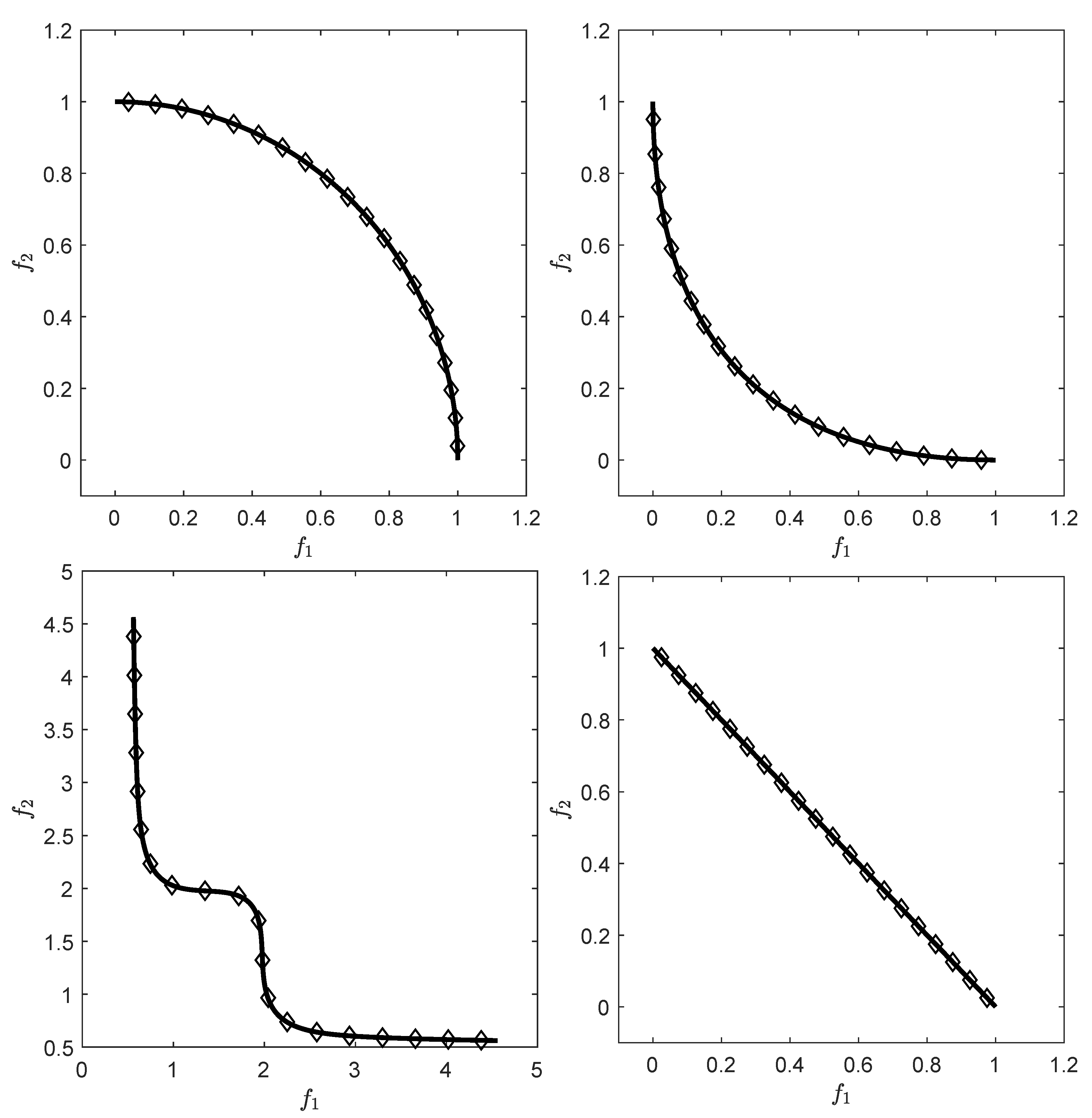
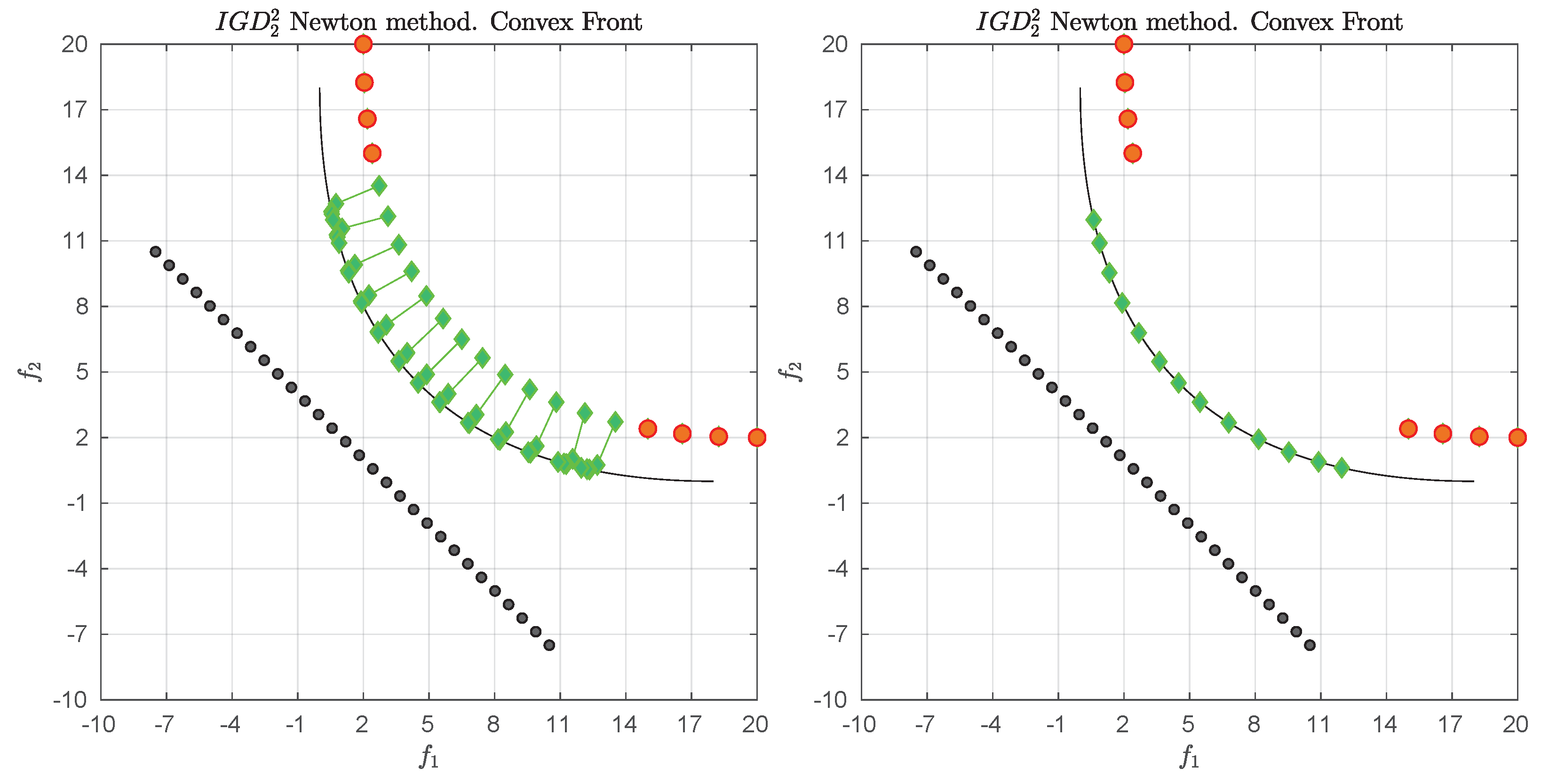
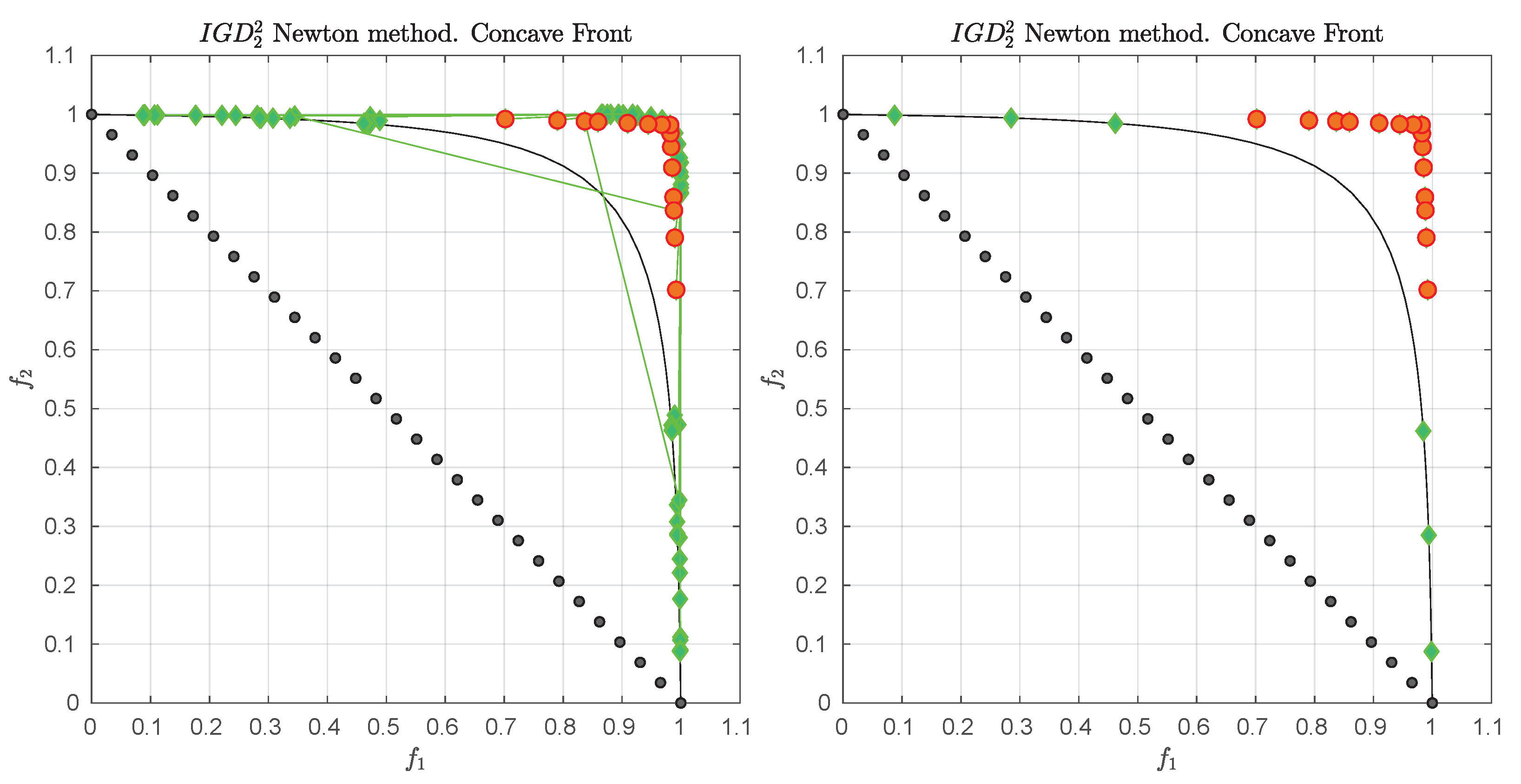
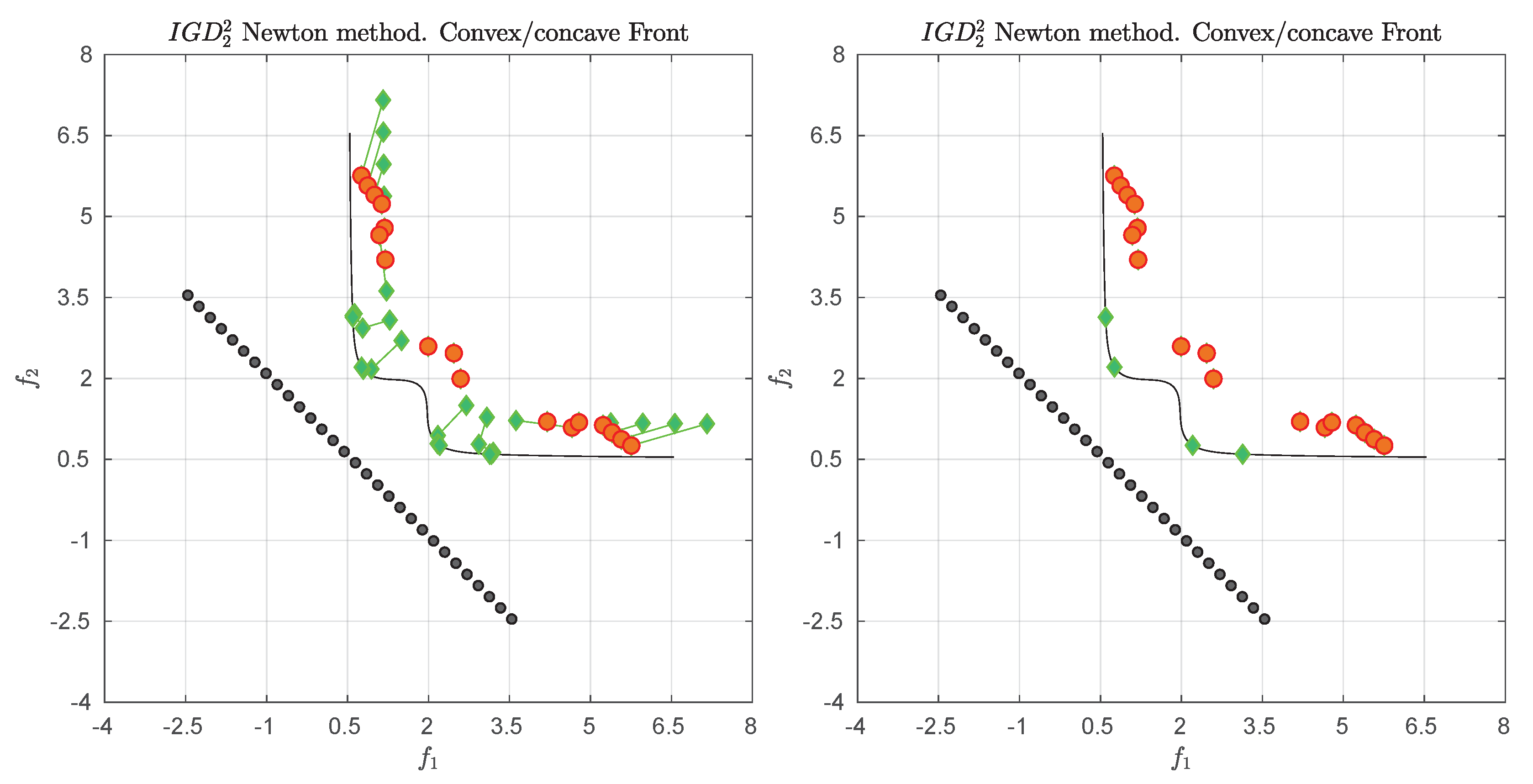
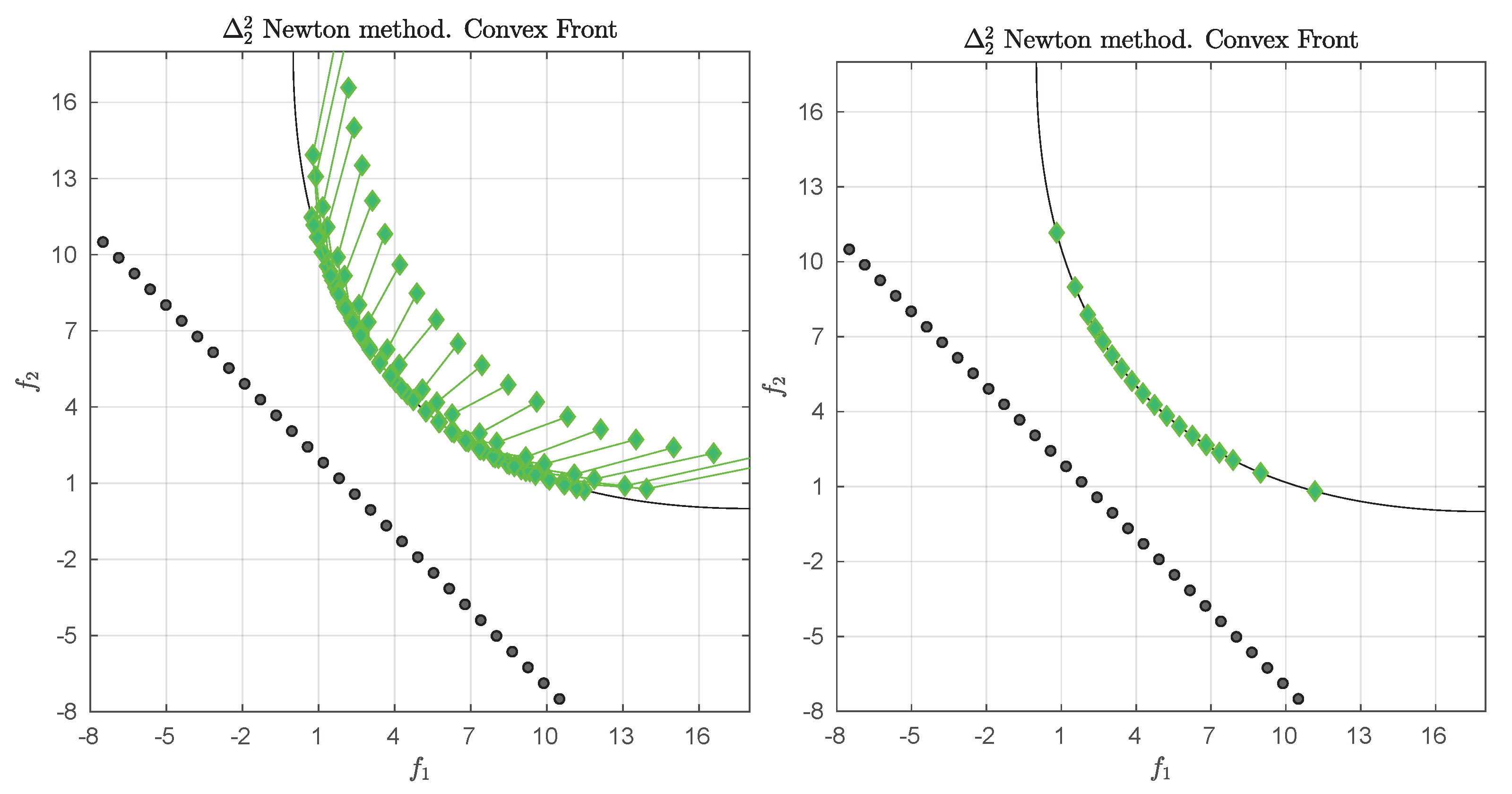
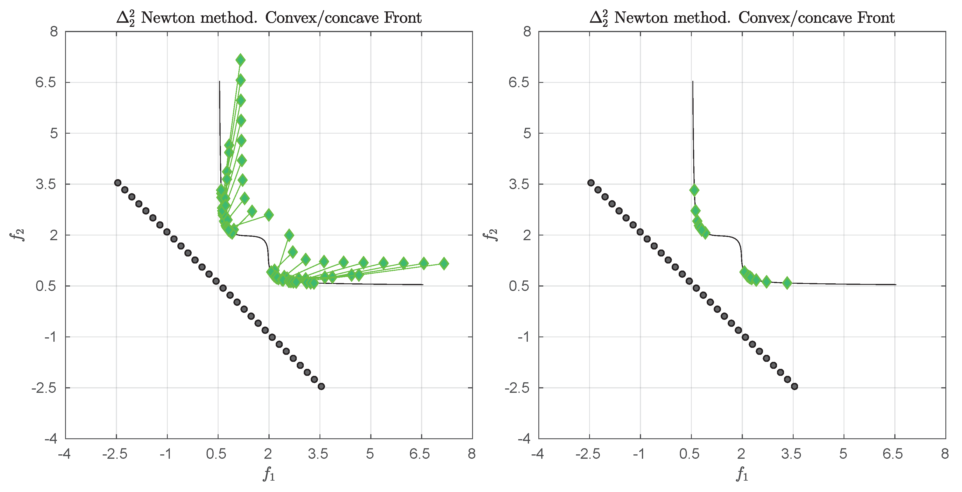
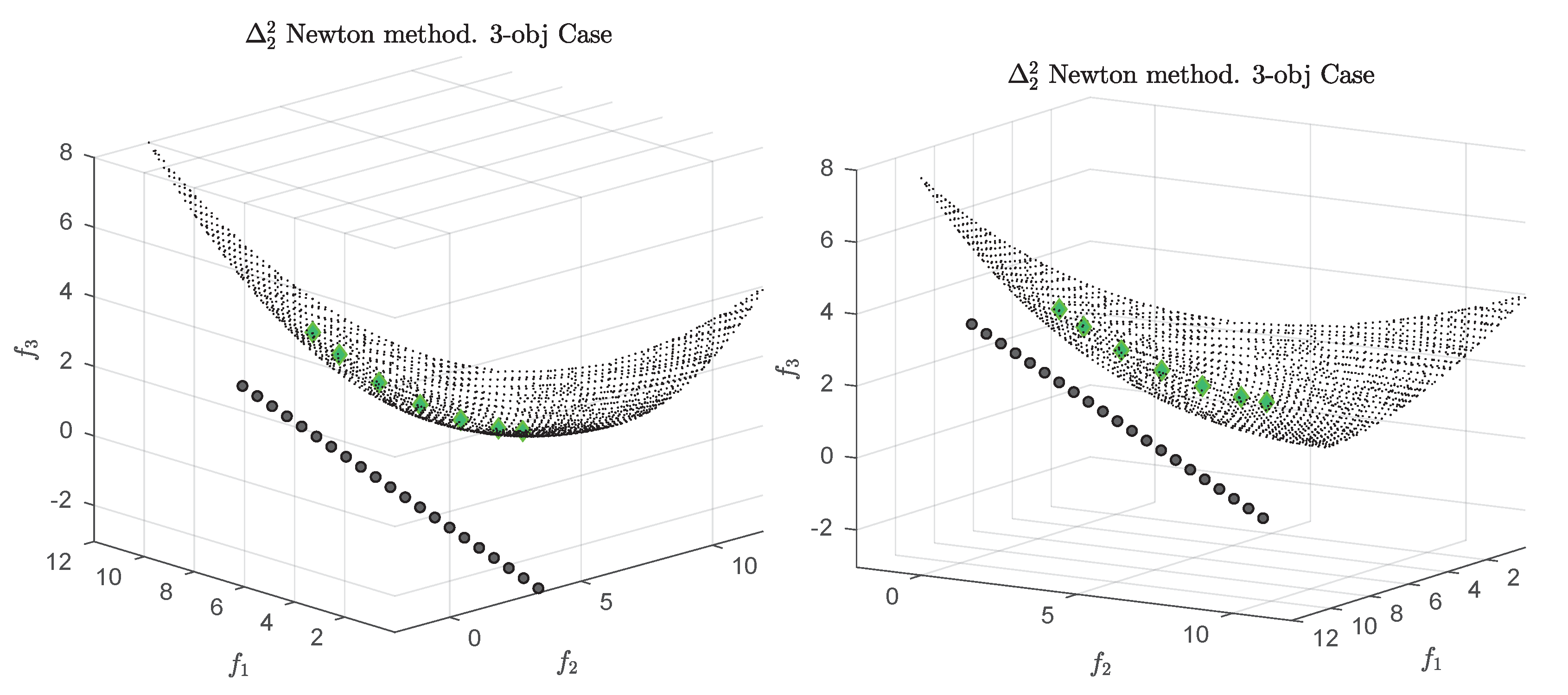
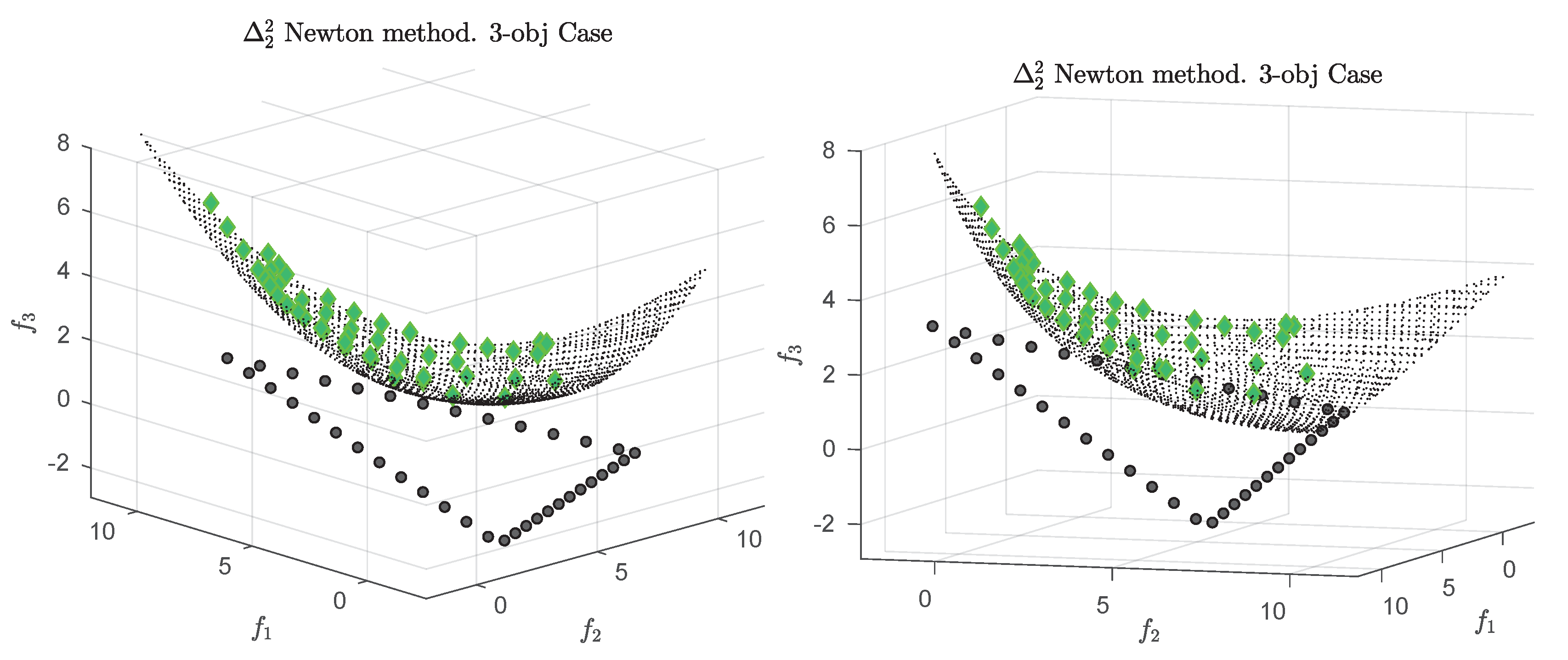
Probably the most important reference set in our context is the Pareto front itself. For this case, ${\mathsf{\Delta }}_p$ prefers, roughly speaking, evenly spread solutions along the Pareto front and is hence e.g., in accord with the terms spread and convergence as used in the evolutionary multi-objective optimization (EMO) community for a “suitable” performance indicator. As an example, Figure 1 shows some “best approximations” in the ${\mathsf{\Delta }}_2$ sense (i.e., when using $p=2$) for MOPs with different shapes of the Pareto front. More precisely, each subfigure shows a fine grain ($M=200$) approximation of the Pareto front of the underlying problem (using dots), as well as the best approximations in the ${\mathsf{\Delta }}_2$ sense (using diamonds). The latter are (numerical) solutions of (5) for $N=20$, and where Z has been chosen as the Pareto front approximation.

If $A=\{a_1,\dots ,a_N\}$ is a subset of the ${\mathbb{R}}^n$ it means that each of its element $a_i$ is an element of the ${\mathbb{R}}^n$. Hence, the set $A=\{a_1,\dots ,a_N\}\subset {\mathbb{R}}^n$ can in a natural way also be identified as a point or vector in the higher dimensional space ${\mathbb{R}}^{N·n}$, i.e., $A\in {\mathbb{R}}^{N·n}$. That is, the optimization problem (5) can be identified as a “classical” scalar optimization problem that is defined in $N·n$-dimensional search space. A necessary condition for optimality is hence given by the Karush–Kuhn–Tucker conditions, e.g., for unconstrained problems we are seeking for sets A for those the (set based) gradient vanishes. In order to solve this root finding problem, one can e.g., utilize the Newton method. If we are given a performance indicator I together with the derivatives $\nabla I\left(A\right)$ and ${\nabla }^{2}I\left(A\right)$ on a set A, the Newton function is hence given by

$$N\left(A\right):=A-{\nabla }^{2}I{\left(A\right)}^{-1}\nabla I\left(A\right).$$

(6)

There exist many methods for the computation of Pareto optimal solutions. For example, there are mathematical programming (MP) techniques such as scalarization methods that transform the MOP into a sequence of scalar optimization problems (SOPs) [22,23,24,25,26]. These methods are very efficient in finding a single solution or even a finite size discretization of the solution set. Another sub-class of the MP techniques is given by continuation-like methods that take advantage of the fact that the Pareto set forms—at least locally—a manifold. Methods of this kind start from a given initial solution and perform a search along the solution manifold [6,27,28,29,30,31,32,33].

Next there exist also set oriented methods that are capable of obtaining the entire solution set in a global manner. Examples for the latter are subdivision [34,35,36] and cell mapping techniques [37,38,39]. Another class of set based methods is given by multi-objective evolutionary algorithms (MOEAs) that have proven to be very effective for the treatment of MOPs [14,16,40,41,42,43]. Some reasons for this include that are very robust, do not require hard assumptions on the model, and allow to compute a reasonable finite size representation of the solution set already in a single run.

Methods that deal with single reference points for multi-objective problems can be found in [26,44,45]. The first work that deals with a set based approach using a problem similar to the one in (5) can be found in [46], where the authors apply the steepest descent method on the Hypervolume indicator [47]. In [48], the Newton method is defined where as well the Hypervolume indicator has been used. In [49], a multi-objective Newton method is proposed that detects single Pareto optimal solutions for a given MOP. In [50], a set based Newton method is proposed for general root finding problems and for convex sets.

3. GD_p Newton Method

In the following sections we will investigate the set based Newton methods for $G{D}_p$, $IG{D}_p$, and ${\mathsf{\Delta }}_p$. More precisely, we will consider the p-th powers, $p>1$, of these indicators as this does not change the optimal solutions. In all cases, we will first derive the (set based) derivatives, and then investigate the resulting Newton method. For the derivatives, we will focus on $p=2$ which is related to the Euclidean norm, and which hence represents the most important performance indicator of the indicator families. However, we will also state the derivatives for general integers p.

Let $A=\{a_1,\dots ,a_N\}\subset {\mathbb{R}}^n$ be a candidate set for (2), and $Z=\{z_1,\dots ,z_M\}\subset {\mathbb{R}}^k$ be a given reference set. The indicator $G{D}_p$ measures the averaged distance of the image of A and Z:

$$G{D}_p\left(A\right):={\left(\frac{1}{N}\sum _{i=1}^{N}d{(F\left(a_i\right),Z)}^p\right)}^{\frac{1}{p}}.$$

(7)

Hereby, we have used the notation

$$d(F\left(a_i\right),Z):=\underset{j=1,\dots ,M}{min}\parallel F\left(a_i\right)-z_j\parallel ,\mathrm{for}i=1,\dots ,N,$$

(8)

and assume Z to be fixed for the given problem (and hence, it does not appear as input argument).

3.1. Derivatives of $G{D}_2^2$

3.1.1. Gradient of $G{D}_2^2$

In the following, we have to assume that for every point $F\left(a_i\right)$ there exists exactly one closest element in Z. That is, $\forall i=1,\dots ,N$ there exists an index $j_i\in \{1,\dots ,M\}$ such that:

$$d(F\left(a_i\right),Z)=\parallel F\left(a_i\right)-z_{j_i}\parallel <\parallel F\left(a_i\right)-z_q\parallel \forall q\in \{1,\dots ,M\}\backslash \left\{j_i\right\}.$$

(9)

Otherwise, the gradient of $G{D}_p$ is not defined at A. If condition (9) is satisfied, then (7) can be written as follows:

$$G{D}_p\left(A\right):={\left(\frac{1}{N}\sum _{i=1}^N{\parallel F\left(a_i\right)-z_{j_i}\parallel }^p\right)}^{\frac{1}{p}},$$

(10)

and for the special case $p=2$ we obtain

$$G{D}_2^2\left(A\right):=\frac{1}{N}\sum _{i=1}^N{\parallel F\left(a_i\right)-z_{j_i}\parallel }_2^2\in {\mathbb{R}}^{n·N}.$$

(11)

The gradient of $G{D}_2^2$ at A is hence given by

$$\nabla G{D}_2^2\left(A\right):=\frac{2}{N}\left(\begin{array}{c}J{\left(a_1\right)}^T(F\left(a_1\right)-z_{j_1})\\ J{\left(a_2\right)}^T(F\left(a_2\right)-z_{j_2})\\ ⋮\\ J{\left(a_N\right)}^T(F\left(a_N\right)-z_{j_N})\end{array}\right)\in {\mathbb{R}}^{n·N},$$

(12)

where $J\left(a_i\right)$ denotes the Jacobian matrix of F at $a_i$ for $i=1,\dots ,N$. We call the vector

$$J{\left(a_i\right)}^T(F\left(a_i\right)-z_{j_i}),i\in \{1,\dots ,N\},$$

(13)

the i-th sub-gradient ( The sub-gradient is defined here as part of the gradient that is associated to an element a of A, and is not equal to the notion of the sub-gradient known in non-smooth optimization. ) of $G{D}_2^2$ with respect to $a_i\in A$. Note that the sub-gradients are completely independent of the location of the other archive elements $a_j\in A$.

If the given MOP is unconstrained, then the first order necessary condition for optimality is that the gradient of $G{D}_2^2$ vanishes. This is the case for a set A if all sub-gradients vanish

$$\nabla G{D}_2^2\left(A\right)=0\iff J{\left(a_i\right)}^T(F\left(a_i\right)-z_{j_i})=0\forall i=1,\dots ,N.$$

(14)

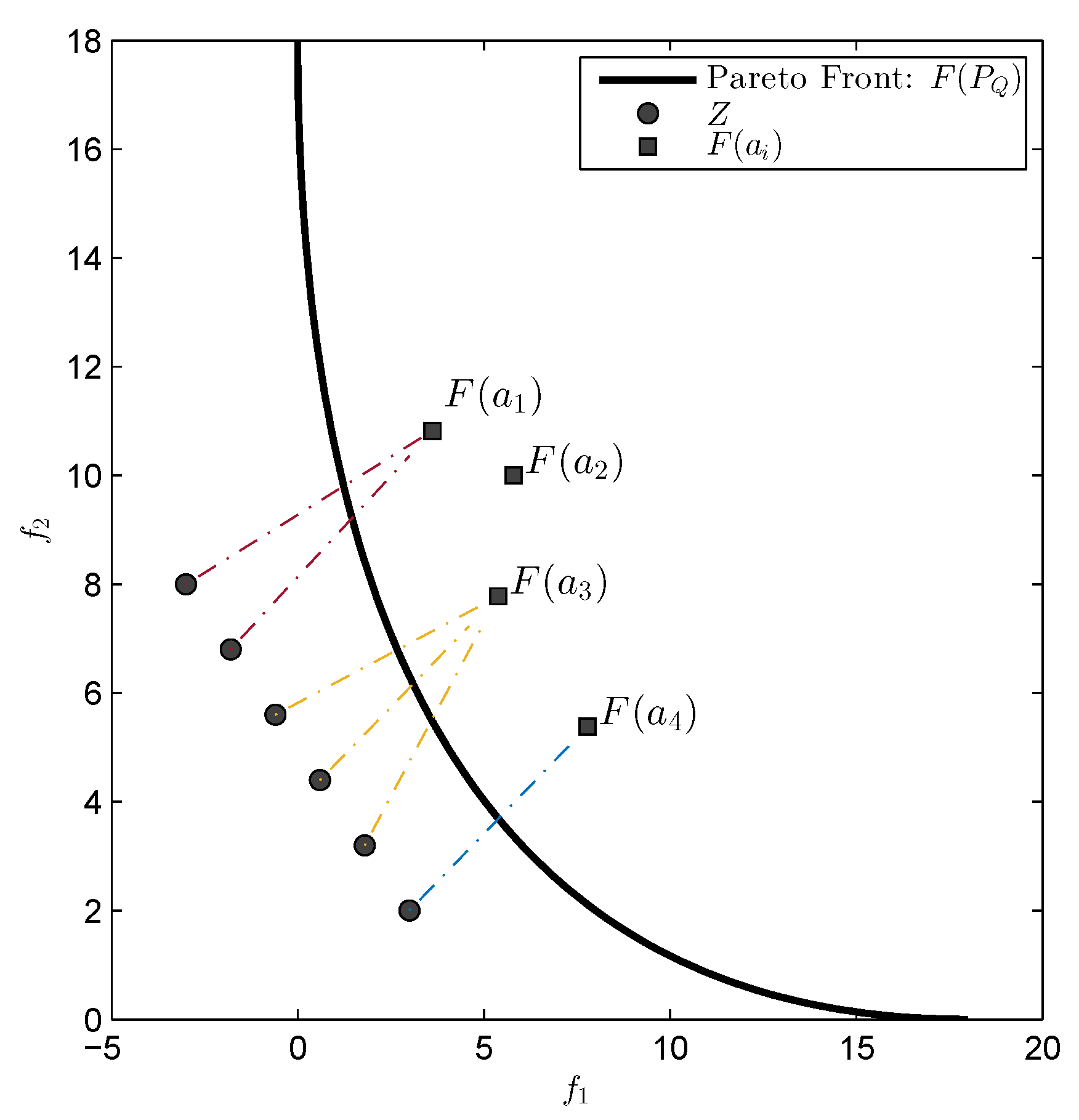
This happens if for each $a_i$ either

(i)

$F\left(a_i\right)=z_{j_i},$ that is, if the image of $a_i$ is equal to one of the elements of the reference set. This is for instance never the case if Z is chosen utopian.

(ii)

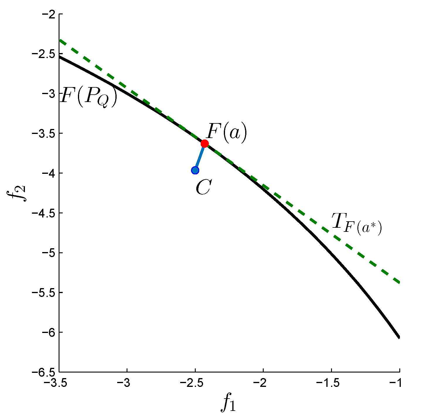
If $F\left(a_i\right)\ne z_{j_i}$, we have

$$J{\left(a_i\right)}^T(F\left(a_i\right)-z_{j_i})=\sum _{l=1}^k\nabla f_l\left(a_i\right)\underset{=:{\alpha }_l^{\left(i\right)}}{\underbrace{(f_l\left(a_i\right)-{\left(z_{j_i}\right)}_l)}}=\sum _{l=1}^k{\alpha }_l^{\left(i\right)}\nabla f_l\left(a_i\right)=0$$

(15)

for a vector ${\alpha }^{\left(i\right)}\in {\mathbb{R}}^k\backslash \left\{0\right\}$. The point $a_i$ is hence a critical point since $rank\left(J\left(a_i\right)\right)<k$. Furthermore, if $F\left(a_i\right)-z_{j_i}{\ge }_{p}0$ (e.g., if Z is again utopian) then $a_i$ is even a Karush–Kuhn–Tucker point. See Figure 2 for a geometrical interpretation of this scenario.

3.1.2. Hessian of $G{D}_2^2$

We first define the map $g:{\mathbb{R}}^n\to {\mathbb{R}}^n$ as

$$g\left(a_i\right):=\sum _{l=1}^k{\alpha }_l^{\left(i\right)}\nabla f_l\left(a_i\right),$$

(16)

where ${\alpha }^{\left(i\right)}$ is as in (15). In order to find an expression of the Hessian matrix, we now derive Equation (16) as follows:

$$\mathcal{D}g\left(a_i\right)=\sum _{l=1}^k\left(\nabla f_l\left(a_i\right)\nabla f_l{\left(a_i\right)}^T+{\alpha }_l{\nabla }^2{f}_l\left(a_i\right)\right)=J{\left(a_i\right)}^{T}J\left(a_i\right)+W_{\alpha }\left(a_i\right)\in {\mathbb{R}}^{n\times n},$$

(17)

where

$$W_{\alpha }\left(a_i\right)=\sum _{l=1}^k{\alpha }_l{\nabla }^2{f}_l\left(a_i\right).$$

(18)

Thus, the Hessian matrix of $G{D}_2^2$ is

$${\nabla }^{2}G{D}_2^2\left(A\right)=\frac{2}{N}\mathrm{diag}\left(\mathcal{D}g\left(a_1\right),\dots ,\mathcal{D}g\left(a_N\right)\right)\in {\mathbb{R}}^{n·N\times n·N},$$

(19)

which is a block diagonal matrix.

3.2. Gradient and Hessian for General $p>1$

As mentioned above, we focus here on the special case $p=2$. The above derivatives, however, can be generalized for $p>1$ as follows (assuming that Z is an utopian finite set to avoid problems when $p<4$): the gradient is given by

$$\nabla G{D}_p^p\left(A\right):=\frac{p}{N}\left(\begin{array}{c}\parallel F\left(a_1\right)-z_{j_1}{\parallel }^{p-2}J{\left(a_1\right)}^T(F\left(a_1\right)-z_{j_1})\\ \parallel F\left(a_2\right)-z_{j_2}{\parallel }^{p-2}J{\left(a_2\right)}^T(F\left(a_2\right)-z_{j_2})\\ ⋮\\ \parallel F\left(a_N\right)-z_{j_N}{\parallel }^{p-2}J{\left(a_N\right)}^T(F\left(a_N\right)-z_{j_N})\end{array}\right)\in {\mathbb{R}}^{n·N},$$

(20)

and the Hessian by

$${\nabla }^{2}G{D}_p^p\left(A\right)=\mathrm{diag}\left({\mathcal{H}}_1,\dots ,{\mathcal{H}}_N\right)\in {\mathbb{R}}^{n·N\times n·N},$$

(21)

where

$$\begin{array}{ccc}\hfill {\mathcal{H}}_i& =& \frac{p(p-2)}{N}{\parallel F\left(a_i\right)-z_{j_i}\parallel }^{p-4}\left[J{\left(a_i\right)}^T(F\left(a_i\right)-z_{j_i}){(F\left(a_i\right)-z_{j_i})}^{T}J{\left(a_i\right)}^T\right]\hfill \\ & & +\frac{p}{N}\left[J{\left(a_i\right)}^{T}J\left(a_i\right)+W_{\alpha }\left(a_i\right)\right],\hfill \end{array}$$

(22)

for $i=1,2,\dots ,N.$

3.3. $G{D}_2^2$-Newton Method

After having derived the gradient and the Hessian we are now in the position to state the set based Newton method for the $G{D}_2^2$ indicator:

The Newton iteration can in practice be stopped at a set $A^f$ if

$$\parallel \nabla G{D}_2^2\left(A^f\right)\parallel \le tol,$$

(24)

for a given tolerance $tol>0$. In order to speed up the computations one may proceed due to the structure of the (sub-)gradient as follows: for each element $a_i$ of a current archive A with

$$\parallel J{\left(a_i\right)}^T(F\left(a_i\right)-z_{j_i})\parallel \le \frac{tol}{\sqrt{N}}$$

(25)

one can continue the Newton iteration with the smaller set $\overline{A}=A\backslash \left\{a_i\right\}$ (and later insert $a_i$ into the final archive).

We are particularly interested in the regularity of ${\nabla }^{2}G{D}_2^2$ at the optimal set, i.e., at a set $A^{*}$ that solves problem (5) for $I=G{D}_2^2$. This is the case since if the Hessian is regular at $A^{*}$—and if the objective function is sufficiently smooth—we can expect the Newton method to converge locally quadratically [51].

Since the Hessian is a block diagonal matrix it is regular if all of its blocks

$$J{\left(a_i\right)}^{T}J\left(a_i\right)+W_{{\alpha }^{\left(i\right)}}\left(a_i\right),i=1,\dots ,N,$$

(26)

are regular. From this we see already that if Z is not utopian, we cannot expect quadratic convergence: assume that one point $z\in Z$ is feasible, i.e., that there exists one $x\in Q$ such that $F\left(x\right)=z$. We can assume that x is also a member of the optimal set $A^{*}$, say $a_i=x$. Then, we have that the weight vector ${\alpha }^{\left(i\right)}$ is zero, and hence that $W_{{\alpha }^{\left(i\right)}}={\sum }_{l=1}^k{\alpha }_l^{\left(i\right)}{\nabla }^2{f}_l\left(a_i\right)=0$. Thus, the block matrix reduces to $J{\left(a_i\right)}^{T}J\left(a_i\right)$ those rank is at most k. The block matrix is hence singular, and so is the Hessian of $G{D}_2^2$ at $A^{*}$.

In the case all individual objectives are strictly convex, the $G{D}_2^2$ Hessian is positive definite (and hence regular) at every feasible set A, and we can hence expect local quadratic convergence.

Proposition 1.

Let a MOP of the form (2) be given whose individual objectives are strictly convex, and let Z be a discrete utopian set. Then, the matrix ${\nabla }^{2}G{D}_2^2\left(A\right)$ is positive definite for all feasible sets A.

Proof. 

Since ${\nabla }^{2}G{D}_2^2\left(A\right)$ is block diagonal, it is sufficient to consider the block matrices $J{\left(a_i\right)}^{T}J\left(a_i\right)+W_{{\alpha }^{\left(i\right)}}\left(a_i\right),i=1,\dots ,N.$ Let $i\in \{1,\dots ,N\}$. Since Z is utopian, it is ${\alpha }^{\left(i\right)}\ne 0$, and all of its elements are non-negative. Further, since all individual objectives $f_l$ are strictly convex, the matrices ${\nabla }^2{f}_l\left(a_i\right)$ are positive definite, and hence also the matrix $W_{\alpha }\left(a_i\right)$. Since $J^T\left(a_i\right)J\left(a_i\right)$ is positive semi-definite, we have for all $x\in {\mathbb{R}}^n\backslash \left\{0\right\}$

$$x^T\left(J{\left(a_i\right)}^{T}J\left(a_i\right)+W_{{\alpha }^{\left(i\right)}}\right)x=x^{T}J{\left(a_i\right)}^{T}J\left(a_i\right)x+x^T{W}_{{\alpha }^{\left(i\right)}}x>0,$$

since $x^{T}J{\left(a_i\right)}^{T}J\left(a_i\right)x\ge 0$ and $x^T{W}_{{\alpha }^{\left(i\right)}}x>0$. Therefore, each $\mathcal{D}g\left(a_i\right)$, $i=1,\dots ,N$, is positive definite and hence also the matrix ${\nabla }^{2}G{D}_2^2\left(A\right)$.  □

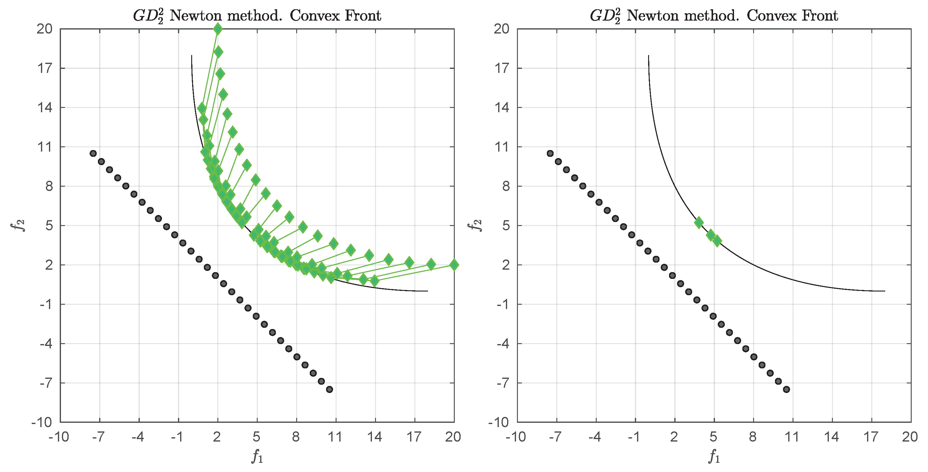
3.4. Example

We consider the following convex bi-objective problem

$$\begin{array}{cc}\hfill f_1,f_2& :{\mathbb{R}}^2\to \mathbb{R}\hfill \\ \hfill f_1\left(x\right)& =x_1^2+{\left(x_2+3\right)}^2\hfill \\ \hfill f_2\left(x\right)& ={(x_1+3)}^2+x_2^2.\hfill \end{array}$$

(27)

Figure 3 shows the Pareto front of this problem together with the reference set Z that contains 30 elements (black dots). The set Z is a discretization of the convex hull of individual minima (CHIM, [23]) of the problem that has been shifted left down. Further, it shows the images of the Newton steps of an initial set $A_0$ that contains 21 elements. As it can be seen, all images converge toward three solutions that are placed in the middle of the Pareto front (which is owed to the fact that Z is discrete. If Z would be continuous, all images would converge toward one solution). This example already shows that the $G{D}_2^2$ Newton method is of restricted interest as standalone algorithm. The method will, however, become important as part of the ${\mathsf{\Delta }}_p$-Newton method as it will become apparent later on.

Table 1. Numerical results of the $G{D}_2^2$-Newton method for BOP (27).

Iter.	$\parallel \mathit{\nabla }{\mathit{GD}}_2^2\left({\mathit{A}}^{\mathit{i}}\right)\parallel$	${\mathit{GD}}_2^2(\mathit{F}\left({\mathit{A}}^{\mathit{i}}\right),\mathit{F}\left({\mathit{P}}_{\mathit{Q}}\right))$	${\mathit{GD}}_2^2(\mathit{F}\left({\mathit{A}}^{\mathit{i}}\right),\mathit{Z})$
0	-	12.000000000000000	2.102524077758237
1	24.575789798441914	2.443855313744088	1.364160070353236
2	10.174108923911083	0.155893831541973	1.099322040004995
3	5.003263195893473	0.002209872937986	1.014751905633911
4	3.169714351377499	0.000015254816873	0.976329099745630
5	1.947602617177173	0.000000021343544	0.957865673825140
6	1.758375206901766	0.000000000020256	0.945790145414235
7	1.433193382521511	0.000000000000013	0.939274242767051
8	1.012249366157551	0.000000000000000	0.936469149315602
9	0.006408088020990	0.000000000000000	0.936469035893491
10	0.000000182419413	0	0.936469035893491
11	0.000000000000002	0	0.936469035893491

shows the respective $G{D}_2^2$ values plus the norms of the gradients which indicate quadratic convergence. The second column indicates that the images of the archives converge toward the Pareto front as anticipated.

4. IGD_p Newton Method

The indicator $IG{D}_p$ computes how far, on average, the discrete reference set Z is from a given archive A, and is defined as

$$IG{D}_p\left(A\right):={\left(\frac{1}{M}\sum _{i=1}^{M}d{(z_i,F\left(A\right))}^p\right)}^{\frac{1}{p}},$$

(28)

where $d(z_i,F\left(A\right))$ is given by

$$d(z_i,F\left(A\right)):=\underset{j=1,\dots ,N}{min}\parallel z_i-F\left(a_j\right)\parallel ,\mathrm{for}i=1,\dots ,M.$$

(29)

4.1. Gradient of $IG{D}_p$

Similar to $GD$, we will also have to assume that for all $i=1,\dots ,M$ there exists an index $j_i\in \{1,\dots ,N\}$ such that:

$$d(z_i,F\left(A\right))=\parallel z_i-F\left(a_{j_i}\right)\parallel <\parallel z_i-F\left(a_q\right)\parallel \forall q\in \{1,\dots ,N\}\backslash \left\{j_i\right\},$$

(30)

since otherwise the gradient of $IG{D}_p$ is not defined. Then, using Equation (30), Equation (28) can be written as follows:

$$IG{D}_p\left(A\right):={\left(\frac{1}{M}\sum _{i=1}^M{\parallel z_i-F\left(a_{j_i}\right)\parallel }^p\right)}^{\frac{1}{p}}.$$

(31)

From now on we will consider $IG{D}_2^2$ which is given by

$$IG{D}_2^2\left(A\right):=\frac{1}{M}\sum _{i=1}^M{\parallel z_i-F\left(a_{j_i}\right)\parallel }_2^2.$$

(32)

In order to derive the gradient of $IG{D}_2^2$, let $I_l:=\{i:j_i=l\}$, $l\in \{1,\dots ,N\}$, be the set formed by the indexes $i\in \{1,2,\dots ,M\}$ that are related to $j_i$. In other words, this set gives us the relation of the elements of Z related to each image $F\left(a_l\right)$ (an example of this relation can be found in Figure 4). Then, the sub-gradient of $IG{D}_2^2$ at point $a_l$ is given by

$$\frac{\partial IG{D}_2^2}{\partial a_l}\left(A\right)=\frac{2}{M}\sum _{i\in I_l}J{\left(a_l\right)}^T(F\left(a_l\right)-z_i)=\frac{2}{M}J{\left(a_l\right)}^T(m_{l}F\left(a_l\right)-\sum _{i\in I_l}{z}_i),$$

(33)

where $m_l=\mid I_l\mid .$ Finally, the gradient of $IG{D}_2^2$ can be expressed as

$$\nabla IG{D}_2^2\left(A\right):=\left(\begin{array}{c}\frac{\partial IG{D}_2^2}{\partial a_1}\left(A\right)\\ \frac{\partial IG{D}_2^2}{\partial a_2}\left(A\right)\\ ⋮\\ \frac{\partial IG{D}_2^2}{\partial a_N}\left(A\right)\end{array}\right)\in {\mathbb{R}}^{n·N}.$$

(34)

It is worth to notice that the sub-gradients depend on the location of the other archive elements which implies a “group motion” (which is in contrast to the gradient of $G{D}_2^2$).

We next consider under which conditions the gradient of $IG{D}_2^2$ vanishes. If $\nabla IG{D}_2^2\left(A\right)=0,$ then for all $l=1,\dots ,N$ we have that

$$\begin{array}{ccc}\hfill J{\left(a_l\right)}^T(m_{l}F\left(a_l\right)-\sum _{i\in I_l}{z}_i)& =& 0\hfill \end{array}$$

(35)

$$\begin{array}{ccc}\hfill \iff J{\left(a_l\right)}^{T}F\left(a_l\right)& =& J{\left(a_l\right)}^T\underset{C_l}{\underbrace{\left(\frac{{\sum }_{i\in I_l}{z}_i}{m_l}\right)}},\hfill \end{array}$$

(36)

where C is the centroid of $z_i$’s. Then, note that if:

• $rank\left(J\left(a_l\right)\right)=k,$ then $F\left(a_l\right)=\frac{{\sum }_{i\in I_l}{z}_i}{m_l}=C_l.$
• $rank\left(J\left(a_l\right)\right)=k-1,$ then $F\left(a_l\right)-C_l$ is orthogonal to the linearized image of F at $F\left(a_l\right)$, and orthogonal to the linearized Pareto front at $F\left(a_l\right)$ in case $F\left(a_l\right)-C_l{\ge }_{p}0$ and $F\left(a_l\right)-C_l\ne 0$ (see Figure 5 for such a scenario).

4.2. Hessian Matrix of $IG{D}_p$

Analog to the derivation of $G{D}_p-$ Hessian, we first define the map $g:{\mathbb{R}}^n\to {\mathbb{R}}^n$ as

$$g\left(a_l\right):=J{\left(a_l\right)}^T(m_{l}F\left(a_l\right)-\sum _{i\in I_l}{z}_i).$$

(37)

Now, let ${\sum }_{i\in I_l}{z}_i=y={\left(y1,\dots ,y_k\right)}^T$. Then

$$g\left(a_l\right)=J{\left(a_l\right)}^T(m_{l}F\left(a_l\right)-y)=m_l\sum _{i=1}^k{f}_i\left(x\right)\nabla f_i\left(x\right)-\sum _{i=1}^k{y}_i\nabla f_i\left(x\right).$$

(38)

Then, we derive Equation (38) as follows:

$$\begin{array}{ccc}\hfill \mathcal{D}g\left(a_l\right)& =& m_l\sum _{i=1}^k{f}_i\left(a_l\right){\nabla }^2{f}_i\left(a_l\right)+m_{l}J{\left(a_l\right)}^{T}J\left(a_l\right)-\sum _{i=1}^k{y}_i{\nabla }^2{f}_i\left(a_l\right)\hfill \\ & =& \sum _{i=1}^k\left(m_l{f}_i\left(a_l\right)-y_i\right){\nabla }^2{f}_i\left(a_l\right)+m_{l}J{\left(a_l\right)}^{T}J\left(a_l\right)\hfill \\ & =& m_{l}J{\left(a_l\right)}^{T}J\left(a_l\right)+W_{\alpha }\left(a_l\right)\in {\mathbb{R}}^{n\times n},\hfill \end{array}$$

(39)

where

$$W_{\alpha }\left(a_l\right)=\sum _{i=1}^k\underset{:={\alpha }_i^{\left(l\right)}}{\underbrace{\left(m_l{f}_i\left(a_l\right)-y_i\right)}}{\nabla }^2{f}_i\left(a_l\right)=\sum _{i=1}^k{\alpha }_i^{\left(l\right)}{\nabla }^2{f}_i\left(a_l\right).$$

(40)

Thus, the Hessian matrix of $IG{D}_2^2$ is given by

$${\nabla }^{2}IG{D}_2^2\left(A\right)=\frac{2}{M}diag\left(\mathcal{D}g\left(a_1\right),\dots ,\mathcal{D}g\left(a_N\right)\right)\in {\mathbb{R}}^{n·N\times n·N},$$

(41)

which is a block diagonal matrix.

4.3. Gradient and Hessian for General $p>1$

The above derivatives can be generalized for $p>1$ as follows: the gradient is given by

$$\nabla IG{D}_p^p\left(A\right):=\frac{p}{M}\left(\begin{array}{c}J{\left(a_1\right)}^T\sum _{i\in I_1}{\parallel F\left(a_1\right)-z_i\parallel }^{p-2}(F\left(a_1\right)-z_i)\\ J{\left(a_2\right)}^T\sum _{i\in I_2}{\parallel F\left(a_2\right)-z_i\parallel }^{p-2}(F\left(a_2\right)-z_i)\\ ⋮\\ J{\left(a_N\right)}^T\sum _{i\in I_N}{\parallel F\left(a_N\right)-z_i\parallel }^{p-2}(F\left(a_N\right)-z_i)\end{array}\right)\in {\mathbb{R}}^{n·N},$$

(42)

and the Hessian by

$${\nabla }^{2}IG{D}_p^p\left(A\right)=\mathrm{diag}\left({\mathcal{H}}_1,\dots ,{\mathcal{H}}_N\right)\in {\mathbb{R}}^{n·N\times n·N},$$

(43)

where

$$\begin{array}{ccc}\hfill {\mathcal{H}}_l& =& \frac{p(p-2)}{N}\sum _{i\in I_l}{\parallel F\left(a_l\right)-z_i\parallel }^{p-4}\left[J{\left(a_l\right)}^T(F\left(a_l\right)-z_i){(F\left(a_l\right)-z_i)}^{T}J{\left(a_l\right)}^T\right]\hfill \\ & & +\frac{p}{M}\left[J{\left(a_l\right)}^{T}J\left(a_l\right)+W_{\alpha }\left(a_l\right)\right].\hfill \end{array}$$

(44)

4.4. $IG{D}_2^2$ Newton Method

After having derived the gradient and the Hessian of $IG{D}_2^2$ we are now in the position to state the respective set based Newton method.

Similarly to the GD Newton method, the iteration can be stopped at an set $A^f$ if

$$\parallel \nabla IG{D}_2^2\left(A^f\right)\parallel \le tol$$

(46)

for a given tolerance $tol>0$, and the iteration for an element $a_i$ can be stopped when

$$\frac{2}{M}J{\left(a_l\right)}^T(m_{l}F\left(a_l\right)-\sum _{i\in I_l}{z}_i)\le \frac{tol}{\sqrt{N}}.$$

(47)

One important special case is when the image $F\left(a_l\right)$ of a point $a_l$ of a set A is not the nearest point of any element of Z, i.e., if $m_l=0$ (see Figure 6). In that case, the l-th sub-gradient vanishes,

$$m_l=0\Rightarrow \frac{\partial IG{D}_2^2}{\partial a_l}\left(A\right)=0,$$

(48)

which means that the point $a_l$ will remain fixed under further iterations of the IGD Newton method. One possibility is hence to neglect such points in subsequent iterations, and to continue with the reduced set. Note also that dominance and distance are two different concepts. That is, if all points of a set A are mutually non-dominated, this does give an implication on $m_l$, see Figure 7 for two examples.

Similar to $GD$, we are interested in the regularity of ${\nabla }^{2}IG{D}_2^2$ at the optimal set since we can in that case expect local quadratic convergence. By the structure of the Hessian we have singularity in the following cases:

• if $m_l=0$ for a $l\in \{1,\dots ,N\}$ (since then $\mathcal{D}g\left(a_l\right)=0$) (see also the discussion above), and
• if one element $z_l$ of Z is feasible (since then $\mathcal{D}g\left(a_l\right)=J{\left(a_l\right)}^{T}J\left(a_l\right)$ which has a rank $\le k$, and under the assumption that $k<n$).

Similar as for $GD$, the $IGD$-Hessian is positive definite for strictly convex problems and utopian reference sets if in addition $m_l\ge 1$ for all $l\in \{1,\dots ,N\}$.

Proposition 2.

Let a MOP of the form (2) be given whose individual objectives are strictly convex, and let Z be a discrete utopian set. Further, let $m_l\ge 1$ for all $l\in \{1,\dots ,N\}$, and A be feasible. Then, the matrix ${\nabla }^{2}IG{D}_2^2\left(A\right)$ is positive definite.

Proof. 

Let $l\in \{1,\dots ,N\}$, and for ease of notation ${\bigcup }_{i\in I_l}{z}_i=\{Z^1,\dots ,Z^{m_l}\}$. Since all $Z^i$’s are utopian we have

$${\alpha }^{\left(l\right)}=m_{l}F\left(a_l\right)-\sum _{i\in I_l}{z}_i=\underset{{\ge }_{p}0}{\underbrace{F\left(a_l\right)-Z^1}}+\cdots +\underset{{\ge }_{p}0}{\underbrace{F\left(a_l\right)-Z^{m_l}}}{\ge }_{p}0,$$

(49)

as well as $m_{l}F\left(a_l\right)\ne {\sum }_{i\in I_l}{z}_i$ (and hence ${\alpha }^{\left(l\right)}\ne 0$). The rest is analog to the proof of Proposition 1.  □

4.5. Examples

We first consider again the convex BOP (27) as for the previous example (see Figure 8), but now using the IGD-Newton method. Already after one iteration step for 8 out of the 21 elements it is $m_l=0$ (denoted by red dots), and we continue the Newton method with the resulting 13-element subset. For this, we obtain quadratic convergence toward the ideal set (for $N=13$) as it can be observed from

Table 2. Numerical results of $IG{D}_2^2$-Newton method for BOP (27), see Figure 8.

Iter.	$\parallel \mathit{\nabla }{\mathit{IGD}}_2^2\left({\mathit{A}}^{\mathit{i}}\right)\parallel$	${\mathit{GD}}_2^2(\mathit{F}\left({\mathit{A}}^{\mathit{i}}\right),\mathit{F}\left({\mathit{P}}_{\mathit{Q}}\right))$	${\mathit{IGD}}_2^2(\mathit{F}\left({\mathit{A}}^{\mathit{i}}\right),\mathit{Z})$
0	-	12.000000000000000	0.280604068205798
1	18.378420484981000	1.930506027522264	0.206869895378755
2	5.432039146770605	0.043471951768718	0.192756253890335
3	0.817043487084936	0.000003701993633	0.192391225092683
4	0.706420510642436	0.000000000171966	0.192326368208389
5	0.006184251273371	0.000000000000000	0.192326331507963
6	0.000000481423311	0	0.192326331505474
7	0.000000000000007	0	0.192326331505474

.

We next consider the following BOP [52]

$$\begin{array}{cc}\hfill f_1,f_2& :{[-4,4]}^2\subset {\mathbb{R}}^2\to \mathbb{R}\hfill \\ \hfill f_1\left(x\right)& =1-exp\left[-{\left(x_1-\frac{1}{\sqrt{2}}\right)}^2-{\left(x_2-\frac{1}{\sqrt{2}}\right)}^2\right]\hfill \\ \hfill f_2\left(x\right)& =1-exp\left[-{\left(x_1+\frac{1}{\sqrt{2}}\right)}^2-{\left(x_2+\frac{1}{\sqrt{2}}\right)}^2\right]\hfill \end{array}$$

(50)

those Pareto front is concave. We apply the IGD-Newton method on the sets $A^0$ with $|A^0|=21$ and Z with $\left|Z\right|=30$ as shown in Figure 9. For this example, only six elements of $A^0$ are closest to one element of Z.

Table 3. Numerical results of $IG{D}_2^2$-Newton method for BOP (50), see Figure 9.

Iter.	$\parallel \mathit{\nabla }{\mathit{IGD}}_2^2\left({\mathit{A}}^{\mathit{i}}\right)\parallel$	${\mathit{IGD}}_2^2(\mathit{F}\left({\mathit{A}}^{\mathit{i}}\right),\mathit{F}\left({\mathit{P}}_{\mathit{Q}}\right))$	${\mathit{IGD}}_2^2(\mathit{F}\left({\mathit{A}}^{\mathit{i}}\right),\mathit{Z})$
0	-	0.278373584606464	0.023220380628487
1	0.336586538953659	0.201027590101253	0.008847986218368
2	0.037592704195443	0.208694136517504	0.008453782829010
3	0.020266018162657	0.205037496184976	0.008317268653462
4	0.004947265003093	0.197436504168332	0.008331864711939
5	0.012675095498115	0.196899482529974	0.008335126593931
6	0.011342458560546	0.195934897889421	0.008256278024484
7	0.001644428661330	0.194957155951972	0.008252791569886
8	0.001355427544721	0.194529344670235	0.008248151529685
9	0.000531420743367	0.194275287179155	0.008247144931520
10	0.000462304446354	0.194197084382389	0.008244551897282
11	0.000160142304221	0.194173320804311	0.008243923138606
12	0.000083987735463	0.194171755397215	0.008243322467470
13	0.000007989306735	0.194171718496160	0.008243262849450
14	0.000000313502013	0.194171718485903	0.008243260421944
15	0.000000004246450	0.194171718485903	0.008243260388981
16	0.000000000077470	0.194171718485903	0.008243260388530
17	0.000000000010284	0.194171718485903	0.008243260388522
18	0.000000000001988	0.194171718485903	0.008243260388521
19	0.000000000000385	0.194171718485903	0.008243260388521
20	0.000000000000075	0.194171718485903	0.008243260388521

shows that the convergence is much slower than for the previous example.

Finally, we consider the BOP [53]

$$\begin{array}{cc}\hfill f_1,f_2& :{\mathbb{R}}^2\to \mathbb{R}\hfill \\ \hfill f_1(x,y)& =\frac{1}{2}\left(\sqrt{1+{(x+y)}^2}+\sqrt{1+{(x-y)}^2}+x-y\right)+\lambda ·e^{-{(x-y)}^2}\hfill \\ \hfill f_2(x,y)& =\frac{1}{2}\left(\sqrt{1+{(x+y)}^2}+\sqrt{1+{(x-y)}^2}-x+y\right)+\lambda ·e^{-{(x-y)}^2}\hfill \end{array}$$

(51)

For $\lambda =0.85$ and $Q={[-1.5,1.5]}^2$ the Pareto front containts a “dent” and is hence convex-concave. Figure 10 shows the setting and

Table 4. Numerical results of $IG{D}_2^2$-Newton method for BOP (51), see Figure 10.

Iter.	$\parallel \mathit{\nabla }{\mathit{GD}}_2^2\left({\mathit{A}}^{\mathit{i}}\right)\parallel$	${\mathit{IGD}}_2^2(\mathit{F}\left({\mathit{A}}^{\mathit{i}}\right),\mathit{F}\left({\mathit{P}}_{\mathit{Q}}\right))$	${\mathit{IGD}}_2^2(\mathit{F}\left({\mathit{A}}^{\mathit{i}}\right),\mathit{Z})$
0	-	0.743479945976417	0.089706026039859
1	1.774223579432539	0.598423777888877	0.069797721774084
2	1.059917072891813	0.580388865733755	0.065730197299576
3	0.436102700877237	0.575606525856331	0.065186338106827
4	0.044524401746943	0.575571396044490	0.065172539475108
5	0.000368536791948	0.575571392056566	0.065172518364193
6	0.000000023167599	0.575571392056566	0.065172518358461
7	0.000000000000001	0.575571392056566	0.065172518358461

the respective convergence behavior. Again, we “lose” elements from $A^0$ since for them there are no elements of Z that are closest to them.

5. ${\mathsf{\Delta }}_{\mathbf{2}}$-Newton Method

Based on the results of the previous two sections we are now in the position to state the set based Newton method for the ${\mathsf{\Delta }}_2^2$ indicator.

5.1. ${\mathsf{\Delta }}_2$-Newton Method

Since ${\mathsf{\Delta }}_2^2(A^i,Z)$ is defined by the maximum of $G{D}_2^2(A^i,Z)$ and $IG{D}_2^2(A^i,Z)$ we simply check in each iteration which of the latter two values is larger, and apply either the $GD$ or the $IGD$-Newton step accordingly.

The properties and the realization of the method are in principle as for the $GD$ and the $IGD$-Newton method. The only difference, at least theoretically, is a possible loss of smoothness since ${\mathsf{\Delta }}_p$ is defined by the maximum of two functions. Such issues, at least for convergence, however, are only to be expected in case $GD(A^{*},Z)$ is equal to $IGD(A^{*},Z)$ for a reference set Z and the respective optimal archive $A^{*}$. The cost for the realization one Newton step for each of the three indicators is $O\left(N{n}^2\right)$ in storage when taking into account the block structure of the Hessians since N matrices of dimension $n\times n$ have to be stored, and $O\left(N{n}^3\right)$ in terms of flops since N linear equation systems of dimension n have to be solved.

5.2. Examples

We will in the following demonstrate the applicability of the ${\mathsf{\Delta }}_2^2$-Newton method on several methods. For this, we first consider the same three examples and settings as for the $IG{D}_2^2$-Newton method presented above. Figure 11, Figure 12 and Figure 13 show some numerical results of the ${\mathsf{\Delta }}_2$-Newton method using the same initial archives $A^0$ and reference sets Z as in the previous section. As it can be seen, in all cases the method achieved much better approximations as for the sole usage of the IGD-Newton method (as well as the GD-Newton method). The convergence behaviors can be seen in

Table 5. Numerical results of the ${\mathsf{\Delta }}_2^2$-Newton method on BOP (27), see Figure 11.

Iter.	$\parallel \mathit{\nabla }{\mathsf{\Delta }}_2^2\left({\mathit{A}}^{\mathit{i}}\right)\parallel$	${\mathsf{\Delta }}_2^2(\mathit{F}\left({\mathit{A}}^{\mathit{i}}\right),\mathit{F}\left({\mathit{P}}_{\mathit{Q}}\right))$	${\mathsf{\Delta }}_2^2(\mathit{F}\left({\mathit{A}}^{\mathit{i}}\right),\mathit{Z})$	Indicator
0	-	2.000000000000000	2.102524077758237	GD
1	24.575789798441914	0.410124138028425	1.364160070353236	GD
2	10.174108923911083	0.026608923543674	1.099322040004995	IGD
3	3.542645526228592	0.000015520657566	1.104000035194028	GD
4	5.213757247004612	0.000000441436988	1.020226507943846	IGD
5	9.260923965020773	0.000000016030350	1.036249331407054	IGD
6	2.625118989394418	0.000000384599061	1.047878336296791	IGD
7	0.042216669617238	0.000000384618980	1.047678945935868	IGD
8	0.000010909557366	0.000000384618980	1.047678891593882	IGD
9	0.000000000000756	0.000000384618980	1.047678891593878	IGD
10	0.000000000000006	0.000000384618980	1.047678891593878	IGD

,

Table 6. Numerical results of the ${\mathsf{\Delta }}_2^2$-Newton method on BOP (50), see Figure 12.

Iter.	$\parallel \mathit{\nabla }{\mathsf{\Delta }}_2^2\left({\mathit{A}}^{\mathit{i}}\right)\parallel$	${\mathsf{\Delta }}_2^2(\mathit{F}\left({\mathit{A}}^{\mathit{i}}\right),\mathit{F}\left({\mathit{P}}_{\mathit{Q}}\right))$	${\mathsf{\Delta }}_2^2(\mathit{F}\left({\mathit{A}}^{\mathit{i}}\right),\mathit{Z})$	Indicator
0	-	0.278373584606464	0.139932582443422	GD
1	0.056371237267200	0.066618294837097	0.056728504338161	GD
2	0.057045938719184	0.039369161609912	0.041433057966044	GD
3	0.037484475625202	0.024109339347752	0.031977133783097	IGD
4	0.050812222533911	0.023513431743364	0.033996922698945	GD
5	0.031160653990564	0.014395303481718	0.024321095970292	IGD
6	0.037264116905168	0.016443622791045	0.025809212757710	IGD
7	0.018144934519792	0.024703492528406	0.029965847813991	IGD
8	0.019468781951843	0.028619439695385	0.030778919683651	GD
9	0.035410330655855	0.017309625336888	0.019853297293327	IGD
10	0.043091325647137	0.021752471483838	0.024124052991424	IGD
11	0.008311561314162	0.017118271463333	0.026490329733338	GD
12	0.029726132461309	0.011015521887052	0.017647857545199	IGD
13	0.049385612870240	0.013547698417436	0.021426583957166	IGD
14	0.014525769797194	0.020436747509906	0.034124722919781	IGD
15	0.030582462613590	0.012480668370491	0.021750946945761	IGD
16	0.030419387651439	0.006090064700256	0.023544581385908	IGD
17	0.012758353366778	0.000030594174296	0.025131789220814	IGD
18	0.009657374280631	0.001454430574110	0.025813967350062	IGD
19	0.005296333332650	0.001374135866037	0.026375698139894	IGD
20	0.005548518084090	0.002112406054454	0.027521017269386	IGD
21	0.005856819919213	0.002804811375528	0.029968509026162	IGD
22	0.012701286040104	0.001922080339960	0.030132357483057	IGD
23	0.003183819547848	0.001504297326063	0.030456038027207	IGD
24	0.003253860331803	0.002240659587601	0.031310708007687	IGD
25	0.003580104890061	0.001602870721889	0.031465842685442	IGD
26	0.002074689422294	0.001367127795787	0.031805380040383	IGD
27	0.001414150903872	0.000126099902661	0.031769100819775	IGD
28	0.001111604812819	0.001688362662578	0.031742469387990	IGD
29	0.000901680741441	0.003036794425943	0.031689031421120	IGD
30	0.000257772611116	0.003797901156449	0.031672123060034	IGD
31	0.000101230696412	0.003991409932376	0.031663374641811	IGD
32	0.000007716198343	0.004008504531546	0.031662626381853	IGD
33	0.000000360445308	0.004008654325951	0.031662593054177	IGD
34	0.000000015185568	0.004008654388153	0.031662591709428	IGD
35	0.000000000643412	0.004008654388154	0.031662591654952	IGD
36	0.000000000027461	0.004008654388154	0.031662591652896	IGD
37	0.000000000001332	0.004008654388154	0.031662591652858	IGD
38	0.000000000000154	0.004008654388154	0.031662591652867	IGD
39	0.000000000000033	0.004008654388154	0.031662591652869	IGD

and

Table 7. Numerical results of the ${\mathsf{\Delta }}_2^2$-Newton method on BOP (51), see Figure 13.

Iter.	$\parallel \mathit{\nabla }{\mathsf{\Delta }}_2^2\left({\mathit{A}}^{\mathit{i}}\right)\parallel$	${\mathsf{\Delta }}_2^2(\mathit{F}\left({\mathit{A}}^{\mathit{i}}\right),\mathit{F}\left({\mathit{P}}_{\mathit{Q}}\right))$	${\mathsf{\Delta }}_2^2(\mathit{F}\left({\mathit{A}}^{\mathit{i}}\right),\mathit{Z})$	Indicator
0	-	0.706541653137130	0.794786137846191	GD
1	2.052766083969590	0.169306894160018	0.477606371056880	GD
2	1.043651307474400	0.001325637478010	0.312621943719186	IGD
3	0.335281361638164	0.000782828935146	0.318925114182142	IGD
4	0.091979632627269	0.000782533520334	0.322156690814970	IGD
5	0.070361802550103	0.000782533238333	0.325270306125291	IGD
6	0.001111027357469	0.000782533238004	0.325312843569155	IGD
7	0.000000574058899	0.000782533238004	0.325312858713113	IGD
8	0.000000000000187	0.000782533238004	0.325312858713118	IGD
9	0.000000000000000	0.000782533238004	0.325312858713118	IGD

. In all cases, the $GD$ value is the greater one in the initial steps of the method. After some iterations (and switches from $GD$ to $IGD$ and vice versa), however, the $IGD$ value becomes eventually the largest one so that the ${\mathsf{\Delta }}_p$-Newton method eventually coincides with the $IGD$-Newton method. In comparison to the results of the $IGD$-Newton method, however, it becomes apparent that the $GD$-Newton steps are in fact important to obtain better overall approximations.

We next consider an example where we use the unconstrained three-objective problem that is defined by the following map

$$\begin{array}{cc}\hfill F:& {\mathbb{R}}^3\to {\mathbb{R}}^3\hfill \\ \hfill F\left(x\right)& =\left(\begin{array}{c}{(x_1+1)}^2+{(x_2+1)}^2+{(x_3+1)}^2\\ {(x_1-1)}^2+{(x_2-1)}^2+{(x_3-1)}^2\\ {(x_1+1)}^2+{(x_2-1)}^2+{(x_3+1)}^2\end{array}\right).\hfill \end{array}$$

(53)

For this problem, we consider the following scenario: assume there are two decision makers which each have their own preference vector (denote here by $z_1={(6.08,-2.08,2.72)}^T$ and $z_2={(0.32,3.68,-3.04)}^T$). As compromise it could be interesting to consider the line segment that connects $z_1$ and $z_2$ (denote by Z) and to compute a set of solutions along the Pareto front that is near (in the Hausdorff sense) to this aspiration set. Figure 14 and

Table 8. Numerical results of ${\mathsf{\Delta }}_2^2$-Newton method for MOP (53), see Figure 14.

Iter.	$\parallel \mathit{\nabla }{\mathsf{\Delta }}_2^2\left({\mathit{A}}^{\mathit{i}}\right)\parallel$	${\mathsf{\Delta }}_2^2(\mathit{F}\left({\mathit{A}}^{\mathit{i}}\right),\mathit{F}\left({\mathit{P}}_{\mathit{Q}}\right))$	${\mathsf{\Delta }}_2^2(\mathit{F}\left({\mathit{A}}^{\mathit{i}}\right),\mathit{Z})$
0	-	1.378676581248260	5.918796450955248
1	7.515915778732357	1.244858568391063	5.821725966611490
2	1.853655193889793	1.249239765031169	5.811343998211261
3	0.145669456936361	1.250137056379269	5.810973507376134
4	0.000671971342724	1.250139614137738	5.810971792145200
5	0.000000033865300	1.250139614289546	5.810971792043552
6	0.000000000000003	1.250139614289546	5.810971792043552

show the numerical result of the Newton method for an initial set consisting of 7 elements. As anticipated, the final set resembles a curve along the Pareto front with minimal distance to Z, and may be used for the decision making process.

This concept can of course be extended to general sets. For instance, one can choose the triangle Z that is defined by the three vertices $z_1={(6.08,-2.08,2.72)}^T$, $z_2={(-2.56,6.56,-0.16)}^T$ and $z_3={(0.20,3.79,-2.92)}^T$ (e.g., if a third decision maker is involved). Figure 15 and

Table 9. Numerical results of ${\mathsf{\Delta }}_2^2$-Newton method for MOP (53) when Z is a triangle, see Figure 15.

Iter.	$\parallel \mathit{\nabla }{\mathsf{\Delta }}_2^2\left({\mathit{A}}^{\mathit{i}}\right)\parallel$	${\mathsf{\Delta }}_2^2(\mathit{F}\left({\mathit{A}}^{\mathit{i}}\right),\mathit{F}\left({\mathit{P}}_{\mathit{Q}}\right))$	${\mathsf{\Delta }}_2^2(\mathit{F}\left({\mathit{A}}^{\mathit{i}}\right),\mathit{Z})$
0	1.000000000000000	1.378676581248260	5.136345894189382
1	9.078968824204878	1.190673858342912	5.014877171961635
2	12.361924917381627	1.250986213036476	3.359444827553141
3	4.188649668005252	1.076592897207513	3.232994469439562
4	0.664877643630374	1.053683832191072	3.217085086974496
5	0.686656379329441	1.036451498535567	3.213854172896627
6	0.005761784413677	1.036607563930994	3.213850773658971
7	0.000001010224622	1.036607573211355	3.213850772877354
8	0.000000000000157	1.036607573211355	3.213850772877354
9	0.000000000000002	1.036607573211354	3.213850772877354

show such a numerical result. For sake of better visualization, we only show the edges Z instead of the complete triangle. As it can be seen, the obtained solutions resemble to a certain extent a bended triangle along the Pareto front. From Table 9 it follows that for the final iteration the value $\parallel \nabla {\mathsf{\Delta }}_2^2\left(A^6\right)\parallel$ is already very close to zero which indicates that a local solution has been computed. The solution, however, does not seem to be perfectly shaped which is due to the fact that the problem to locate solutions along the Pareto front with respect to the given reference set is highly multi-modal (the “perfect” shape is associated to the global solution of Problem (5)). In order to obtain better results it is hence imperative to hybridize the set based Newton methods with global multi-objective solvers (as e.g., multi-objective evolutionary algorithms) which is beyond the scope of this work.

5.3. A Bootstrap Method for the Computation of the Pareto Front

It is known that the proper choice of reference points/sets is a non-trivial task for the use of performance indicators in general when targeting at the entire solution set (e.g., [54,55,56]). In the following we show some numerical results of a bootstrap method that allows to a certain extent to compute approximations of the entire Pareto fronts of a given MOP without prior knowledge of this set. For this, we adapt the idea proposed in [57] to the context of the set based Newton method: given a performance indicator and a set based SOP of the form (5), one can iteratively approximate the Pareto front of a given problem using the Newton method via the following steps:

• Compute the minima $x_i^{*}$ of the individual objectives $f_i$, $i=1,\dots ,k$. Let $y_i^{*}=F\left(x_i^{*}\right)$, and let ${\tilde{Z}}_0$ be the convex hull of the $y_i^{*}$’s (also called convex hull of individual minima (CHIM) [23]). Let ${\delta }_0>0$ and set

  $$Z_0={\tilde{Z}}_0-{\delta }_0,$$

  (54)

  where ${\delta }_0$ is ideally large enough so that $Z_0$ is utopian. Compute a Newton step using $Z_0$ leading to the set of candidate solutions $A^{\left(0\right)}$.
• In step l of the iteration, use the set $A^{(l-1)}$ computed in the previous iteration to compute a set ${\tilde{Z}}_l$. This can be done via interpolation of the elements of $A^{(l-1)}$ so that ${\tilde{Z}}_l$ only contains mutually non-dominated elements. As new reference set use

  $$Z_l={\tilde{Z}}_l-{\delta }_l,$$

  (55)

  where ${\delta }_l<{\delta }_{l-1}$. Compute a Newton step using $Z_l$ leading to $A^{\left(l\right)}$.

For $k=2$ objectives, the CHIM is simply the line segment that connects $y_1^{*}$ and $y_2^{*}$. Figure 16, Figure 17 and Figure 18 and

Table 10. Numerical results of the ${\mathsf{\Delta }}_2^2$-Newton method to obtain the Pareto front of MOP (27) via the bootstrapping method.

Iter.	$\parallel \mathit{\nabla }{\mathsf{\Delta }}_2^2\left({\mathit{A}}^{\mathit{i}}\right)\parallel$	${\mathsf{\Delta }}_2^2(\mathit{F}\left({\mathit{A}}^{\mathit{i}}\right),\mathit{F}\left({\mathit{P}}_{\mathit{Q}}\right))$	${\mathsf{\Delta }}_2^2(\mathit{F}\left({\mathit{A}}^{\mathit{i}}\right),\mathit{Z})$	Indicator
0	-	2.565838356405802	5.454852860388515	GD
1	14.958401000284267	1.230817708101819	1.024752009175881	IGD
2	6.553591835159349	0.754749784421640	0.553744685923295	IGD
3	1.930428808338138	0.613768117290251	0.490492908923838	IGD
4	0.937132679630156	0.537139549603782	0.481517242208329	IGD
5	0.540200357139832	0.476989307368074	0.471988242018486	IGD
6	0.394304493982539	0.438480476946482	0.467546882767516	IGD
7	0.153675036875927	0.419941366901776	0.468192970378975	IGD
8	0.059462724070887	0.413040100805383	0.468716613758660	IGD
9	0.039636672484473	0.412237873646849	0.468845106760589	IGD
10	0.016104664984103	0.412336536272929	0.468844846612736	IGD
11	0.001970967225026	0.412348016205662	0.468845003745375	IGD
12	0.000010540592599	0.412348100926435	0.468845005883349	IGD
13	0.000000006447819	0.412348100981951	0.468845005884675	IGD
14	0.000000000000000	0.412348100981951	0.468845005884675	IGD

,

Table 11. Numerical results of the ${\mathsf{\Delta }}_2^2$-Newton method to obtain the Pareto front of MOP (50) via the bootstrapping method.

Iter.	$\parallel \mathit{\nabla }{\mathsf{\Delta }}_2^2\left({\mathit{A}}^{\mathit{i}}\right)\parallel$	${\mathsf{\Delta }}_2^2(\mathit{F}\left({\mathit{A}}^{\mathit{i}}\right),\mathit{F}\left({\mathit{P}}_{\mathit{Q}}\right))$	${\mathsf{\Delta }}_2^2(\mathit{F}\left({\mathit{A}}^{\mathit{i}}\right),\mathit{Z})$	Indicator
0	-	0.455981539616886	0.695079920183452	GD
1	0.335395116261223	0.073901038363798	0.755243658407092	GD
2	0.091052248527535	0.037763808963224	0.074896196233522	IGD
3	0.014233219389476	0.037763808963224	0.037618719614753	IGD
4	0.012918924846453	0.037763808963224	0.037607435705178	IGD
5	0.012918504651879	0.037763808963224	0.037607435705178	IGD

and

Table 12. Numerical results of the ${\mathsf{\Delta }}_2^2$-Newton method to obtain the Pareto front of MOP (51) via the bootstrapping method.

Iter.	$\parallel \mathit{\nabla }{\mathsf{\Delta }}_2^2\left({\mathit{A}}^{\mathit{i}}\right)\parallel$	${\mathsf{\Delta }}_2^2(\mathit{F}\left({\mathit{A}}^{\mathit{i}}\right),\mathit{F}\left({\mathit{P}}_{\mathit{Q}}\right))$	${\mathsf{\Delta }}_2^2(\mathit{F}\left({\mathit{A}}^{\mathit{i}}\right),\mathit{Z})$	Indicator
0	-	0.702540625580303	2.214433876989687	GD
1	1.437150990002929	0.389087697290865	0.477018278137838	IGD
2	0.581565628190262	0.342604825739356	0.357844471083072	IGD
3	0.461927350893728	0.164460636656196	0.182910255512032	IGD
4	0.082455998873464	0.158481979725082	0.175440371075156	IGD
5	0.074464658261760	0.191541386471772	0.208964468823487	IGD
6	0.131398860002112	0.153900963788386	0.171965063484733	IGD
7	0.040291187202238	0.152033891842905	0.166135305826676	IGD
8	0.005689443259245	0.151817516262598	0.165264799265542	IGD
9	0.002103237914802	0.151819267034376	0.165273277734145	IGD
10	0.000466641874904	0.151819600203537	0.165273337507943	IGD
11	0.000013655772453	0.151819670338732	0.165273320812711	IGD
12	0.000000209461574	0.151819687437130	0.165273316697773	IGD
13	0.000000050653504	0.151819691559064	0.165273315706448	IGD
14	0.000000012209033	0.151819692552588	0.165273315467506	IGD
15	0.000000002942920	0.151819692792067	0.165273315409911	IGD
16	0.000000000709377	0.151819692849792	0.165273315396027	IGD
17	0.000000000167849	0.151819692849792	0.165273315396027	IGD

show the results of this bootstrapping method on the MOPs (27), (50), and (51), respectively.

Table 13. Number of function ($\#F$), Jacobian ($\#J$), and Hessian ($\#H$) calls used by the ${\mathsf{\Delta }}_2^2$-Newton method using bootstrapping for the three test problems.

	MOP (27)	MOP (50)	MOP (51)
$\#F$	532	225	698
$\#J$	532	210	680
$\#H$	513	189	660

shows the number of function, Jacobian, and Hessian calls that have been spent for each problem. In our computations, we have chosen ${\delta }_0$ sufficiently large, and ${\delta }_l=\frac{1}{2}{\delta }_{l-1}$ for the shift parameter. The results show that the entire Pareto fronts can for these examples be approximated via using the Newton method together with the bootstrapping method. While the final approximations can considered to be “good” for the problems with the convex and convex/concave Pareto fronts, the final solution for MOP (50) that contains a concave Pareto front is not yet satisfying. Table 11 indicates that the solutions do not even converge toward a local solution (even if more iteration steps are performed). We conjecture that the problem results from the multi-modality of the test function which encourages us further to hybridize the set based Newton method with a global strategy in the future.

We finally consider a BOP with higher dimensional decision variable space: the bi-objective problem minus DTLZ2 [58] is defined as

$$\begin{array}{cc}\hfill f_1\left(x\right)& =-(1+g\left(x\right))cos\left(\frac{\pi }{2}{x}_1\right)\hfill \\ \hfill f_2\left(x\right)& =-(1+g\left(x\right))sin\left(\frac{\pi }{2}{x}_1\right)\hfill \\ \hfill g\left(x\right)& =\sum _{i=1}^n{(x_i-0.5)}^2,\hfill \end{array}$$

(56)

where we have chosen $n=20$. Figure 19 shows an initial candidate set as well as the final result of the Newton method together with the bootstrapping. In order to obtain the final result, 8 iteration steps were needed using 1415 function, 700 Jacobian, and 350 Hessian calls. Note that the initial set contains some dominated solutions that do not have an influence on the $IG{D}_2$ value. Hence, also in this case the use of $G{D}_2$ helped to push these solutions toward the Pareto front.

6. Conclusions and Future Work

In this work, we have considered a set based Newton Method for the ${\mathsf{\Delta }}_p$ indicator for unconstrained multi-objective optimization problems. Since ${\mathsf{\Delta }}_p$ is constructed by $G{D}_p$ and $IG{D}_p$ we have also considered the set based Newton method for these two indicators. To this end, we have first derived the set based gradients and Hessians, and have based on this formulated and analyzed the Newton methods. Numerical results on selected test problems have revealed the strengths and weaknesses of the resulting methods. For this, we have mainly considered aspiration set problems (i.e., the problem to minimize the indicator distance of a set to a given utopian reference set) but also shown a bootstapping method that allows to a certain extend to compute finite size approximation of the entire Pareto front without prior knowledge of this set. The results have shown that the method may indeed converge quadratically to the desired set, however, also—and as anticipated—that the Newton method is only applicable locally. It is hence imperative to hybridize the method with a global search strategy such as an evolutionary multi-objective optimization algorithm in order to obtain a fast and reliable algorithm for the treatment of such problems. The latter, however, is beyond the scope of this work and left for future investigations. Another interesting path for future research would be to extend the proposed Newton methods to constrained multi-objective optimization problems.