Effect of the Direction of Uniform Horizontal Magnetic Field on the Linear Stability of Natural Convection in a Long Vertical Rectangular Enclosure

Abstract

The effect of the direction of external horizontal magnetic fields on the linear stability of natural convection of liquid metal in an infinitely long vertical rectangular enclosure is numerically studied. A vertical side wall is heated and the opposing vertical wall is cooled both isothermally, whereas the other two vertical walls are adiabatic. A uniform horizontal magnetic field is applied either in the direction parallel or perpendicular to the temperature gradient. In this study, the height of the enclosure is so long as to neglect the top and bottom effects where returning flow takes place, and thus the basic flow is assumed to be a parallel flow and the temperature field is in heat conduction state. The Prandtl number is limited to the value of 0.025 and horizontal cross-section is square. The natural convection is monotonously stabilized as increase in the Hartmann number when the applied magnetic field is parallel to the temperature gradient. However, when the applied magnetic field is perpendicular to the temperature gradient, it is once destabilized at a certain low Hartmann number, but it is stabilized at high Hartmann numbers.

1. Introduction

Control of the heat transfer and fluid flow of molten metal is essential in various industrial fields such as semiconductor single crystal growth of semiconductors and continuous casting of steel making process. One of such control methods is to apply an external magnetic field to the molten metal flows. By applying a magnetic field, the flow field itself is greatly affected by the electromagnetic force in the liquid metal [1,2,3]. Normally, since the Prandtl number of liquid metal is very small, the flow field tends to be turbulent at high Rayleigh numbers, but the turbulence in the flow field is stabilized by applying a magnetic field. Because of this principle, many theoretical, numerical, and experimental studies in which magnetic fields are applied to the natural convection of liquid metals in enclosures can be found. There are various types of natural convection, such as the Rayleigh–Bénard convection (a horizontal fluid layer is heated from below and cooled from above), convection heated and cooled from the vertical surfaces of the container, natural convection in inclined enclosures, natural convection caused by internal heat generation, etc. The Boussinesq approximation is often used for the analysis of natural convection, and it is known that when the boundary condition has symmetry, the flow and temperature fields also have symmetry. When assuming the Boussinesq approximation, the Nusselt number can be obtained based on the temperature field data by using two independent parameters among the Rayleigh number, the Prandtl number, and the Grashof number.

Concerning MHD (magnetohydrodynamics) natural convection, most of these studies are roughly divided into those in shallow horizontal enclosures and those in the vertical slots. Chandrasekhar’s textbook [4] discusses the stability of a magnetic field applied to Rayleigh–Bénard convection. In recent years, Burr and Müller [5,6] have investigated the effects of both vertical and horizontal magnetic fields on Rayleigh–Bénard convection. Mistrangelo and Bühler [7] discussed the effect of a horizontal magnetic field on a horizontal fluid layer in the presence of internal heat generation.

On the other hand, in the case of long vertical slots, researches have been conducted since the end of the 1960s. In the case that the effects of the magnetic field are not included, Vest and Arpaci [8] studied natural convection in a vertical slot. Hart [9] dealt with inclined slots. Bergholz [10] considered the case of thermal stratification, Choi and Korpela [11] studied the stability of the heat conduction state of the vertical annulus, and Lee and Korpela [12] performed nonlinear numerical computations with various changes in the aspect ratio of the vertical enclosure and the Prandtl number. Chen and Pearlstein [13] investigated the stability of natural convection of variable-viscosity fluid in inclined slots. Various studies have been still continued since the 1990s [14,15,16,17,18,19,20].

Studies that do not use the Boussinesq approximation have become important because of the large temperature gradient to destabilize natural convection in a slot as the electric heating equipment becomes smaller. Suslov and Paolucci [21] investigated the stability of natural convection in vertical slots without use of the Boussinesq approximation. Kitada et al. [22] then discussed the inclined slots using the same equations employed by Suslov and Paolucci [21].

As studies considering the influence of the magnetic field, there are the ones by Takashima [23] and by Nagata [24], which are two-dimensional computations. An experimental study was made by Burr et al. [25]. In recent years, Hudoba and Molokov [26] has studied a stability analysis of the natural convection due to the internal heating.

The study of three-dimensional vertical natural convection is important in relation to the liquid metal blanket problem of fusion reactors [27,28]. Tagawa et al. [29], with assuming that the container is infinite length, compared the theoretical solution of parallel flow with the numerical solution using the Hartmann boundary layer approximation and confirmed that they agreed quite well to each other. Then, Authié et al. [30] made experiments using mercury and three-dimensional numerical simulations in a container of finite height (aspect ratio 7.5), and the two were compared. They found two main findings in their researches. One is that the flow damping effect significantly depends on the direction of the applied magnetic field, and the other is that the Nusselt number rises slightly when a weak magnetic field is applied in the Y-direction (perpendicular to temperature gradient).

As a stability analysis of three-dimensional natural convection, Lyubimov et al. [31] dealt with shear flow instability in a horizontally long rectangular enclosure. Kitaura and Tagawa [32] have conducted a linear stability analysis for the case of Tagawa et al. [29] as the basic state, but the direction of the magnetic field was limited to the Y-direction only. The influence of the uniform magnetic field applied in X-direction and that in the intermediate direction between these two typical cases was not discussed. It should be noted that, as reported in the reference of Tagawa et al. [29], when a magnetic field was applied in the X- or Y-direction, its basic state such as vertical velocity, current density, and electric potential had two-fold line symmetry within a horizontal cross-section of the enclosure. However, when the magnetic field is applied from an oblique direction, the basic state is partially distorted and it exhibits rotational symmetry, which may affect the stability of such MHD flow. Therefore, the purpose of this study is to clarify the linear stability of natural convection under a uniform horizontal magnetic field considering the direction of the magnetic field.

2. Governing Equations

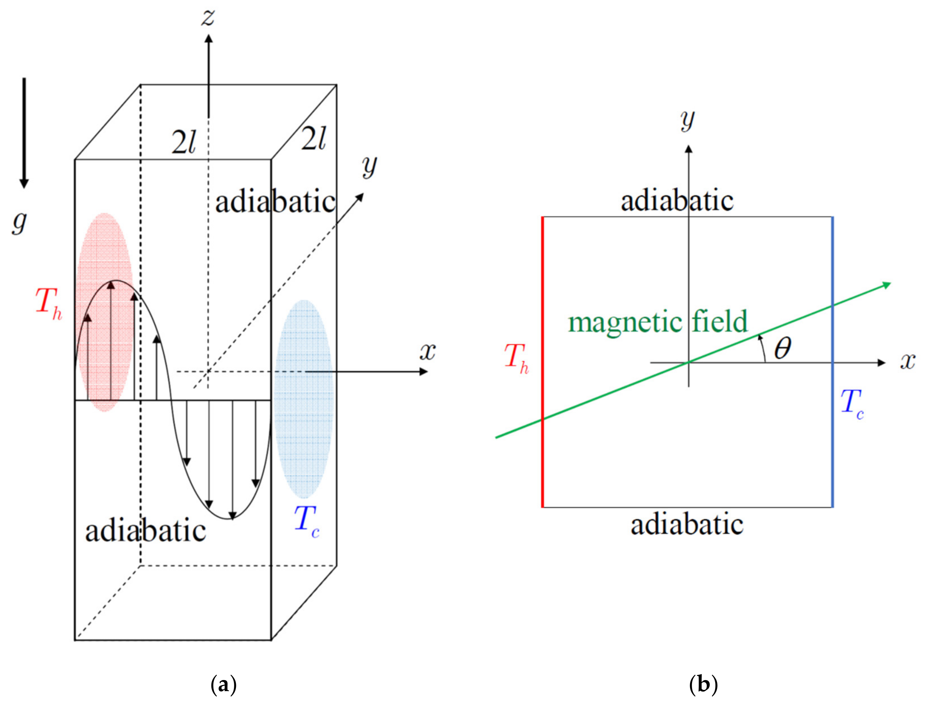
The author considers natural convection in a vertically long rectangular container with a square horizontal cross-section, whose vertical surface of the container is heated at a constant temperature, and the opposing vertical surface is cooled at a constant temperature, whereas the other two vertical walls are assumed to be adiabatic as shown in Figure 1. The applied magnetic field is horizontal and uniform, and either a magnetic field parallel to the temperature gradient (X-directional magnetic field) or a magnetic field perpendicular to the temperature gradient (Y-directional magnetic field) is examined. The liquid metal in the container is assumed to be an incompressible Newtonian fluid, and the Boussinesq approximation holds. The viscous dissipation and the Joule heat are ignored. Moreover, since the magnetic Prandtl number is considered to be sufficiently small, the induced magnetic field is neglected compared to the applied magnetic field.

The governing equations are the continuity equation, the equation of motion, the energy equation, the equation of conservation of charge, and the Ohm’s law. The dimensionless governing equations are shown below.

$$\frac{\partial U_j}{\partial X_j}=0$$

(1)

$$\frac{\partial U_i}{\partial \tau }+U_j\frac{\partial U_i}{\partial X_j}=\frac{1}{Gr}\left(-\frac{\partial P}{\partial X_i}+\frac{{\partial }^2{U}_i}{\partial X_j\partial X_j}+H{a}^2{\epsilon }_{ijk}{J}_j{B}_k+\Theta {\delta }_{i3}\right)$$

(2)

$$\frac{\partial \Theta }{\partial \tau }+U_j\frac{\partial \Theta }{\partial X_j}=\frac{1}{GrPr}\frac{{\partial }^2\Theta }{\partial X_j\partial X_j}$$

(3)

$$\frac{\partial J_j}{\partial X_j}=0$$

(4)

$$J_i=-\frac{\partial \Phi }{\partial X_i}+{\epsilon }_{ijk}{U}_j{B}_k.$$

(5)

The dimensionless variables and nondimensional numbers are defined as follows:

$$\begin{array}{l}\tau =\frac{t}{l^2/\left(Gr\nu \right)},\hspace{1em}{X}_i=\frac{x_i}{l},\hspace{1em}{U}_i=\frac{u_i}{Gr\nu /l},\hspace{1em}P=\frac{p}{Gr{\rho }_0{\nu }^2/l^2},\hspace{1em}\mathsf{\Delta }T=\frac{1}{2}\left(T_h-T_c\right),\\ T_0=\frac{1}{2}\left(T_h+T_c\right),\hspace{1em}\Theta =\frac{T-T_0}{\mathsf{\Delta }T},\hspace{1em}{B}_i=\frac{b_i}{b_0},\hspace{1em}{J}_i=\frac{j_i}{Gr\hspace{0.17em}\nu b_0},\hspace{1em}\Phi =\frac{\varphi }{Gr\hspace{0.17em}\sigma \nu b_0/l},\hspace{1em}\\ Gr=\frac{g\beta \mathsf{\Delta }T{l}^3}{{\nu }^2},\hspace{1em}Pr=\frac{\nu }{\alpha },\hspace{1em}Ha=b_{0}l\sqrt{\frac{\sigma }{{\rho }_0\nu }}\end{array}$$

(6)

3. Numerical Analyses of Basic Flows

In this study, it is assumed that the vertically long rectangular container is infinitely long in the vertical direction. Hence, the influence of the upper and lower ends of the container is ignored, the flow is considered to be a parallel flow, and the temperature distribution is in a heat conductive state. In order to obtain such a basic state, it is reduced to solve the following equation of motion, the law of conservation of charge, and Ohm’s law in a certain horizontal cross-section. An overbar is attached to the variables in the basic state.

$$\left(\frac{{\partial }^2}{\partial X^2}+\frac{{\partial }^2}{\partial Y^2}\right)\overline{W}+H{a}^2\left({\overline{J}}_X{B}_Y-{\overline{J}}_Y{B}_X\right)+\overline{\Theta }=0$$

(7)

$$\left(\frac{{\partial }^2}{\partial X^2}+\frac{{\partial }^2}{\partial Y^2}\right)\overline{\Theta }=0$$

(8)

$$\frac{\partial {\overline{J}}_X}{\partial X}+\frac{\partial {\overline{J}}_Y}{\partial Y}=0$$

(9)

$${\overline{J}}_X=-\frac{\partial \overline{\Phi }}{\partial X}-\overline{W}{B}_Y,\hspace{1em}{\overline{J}}_Y=-\frac{\partial \overline{\Phi }}{\partial Y}+\overline{W}{B}_X$$

(10)

$$B_X{}^2+B_Y{}^2=1.$$

(11)

In Equation (11), if (B_X, B_Y) = (1,0), it represents the X-directional magnetic field, and if (B_X, B_Y) = (0,1), it represents the Y-directional magnetic field. Furthermore, if this condition is satisfied, an arbitrary horizontal magnetic field can be applied.

The boundary conditions for the vertical velocity are noslip at the surrounding four walls, and those for the temperature are constants kept at different temperatures at X = −1 and 1 and adiabatic at Y = −1 and 1. The boundary conditions for the electric current density are assumed to be electrically insulated.

$$\left\{\begin{array}{l}X=\pm 1:\hspace{1em}\overline{W}=0,\hspace{1em}\overline{\Theta }=\mp 1,\hspace{1em}{\overline{J}}_X=0\\ Y=\pm 1:\hspace{1em}\overline{W}=0,\hspace{1em}\frac{\partial \overline{\Theta }}{\partial Y}=0,\hspace{1em}{\overline{J}}_Y=0\end{array}\right..$$

(12)

Note that the basic state is nondimensionalized so that it does not depend on the Grashof number, as seen in Equations (7)–(12). This consideration makes it easier to obtain the critical Grashof number when solving the linearized disturbance equation later.

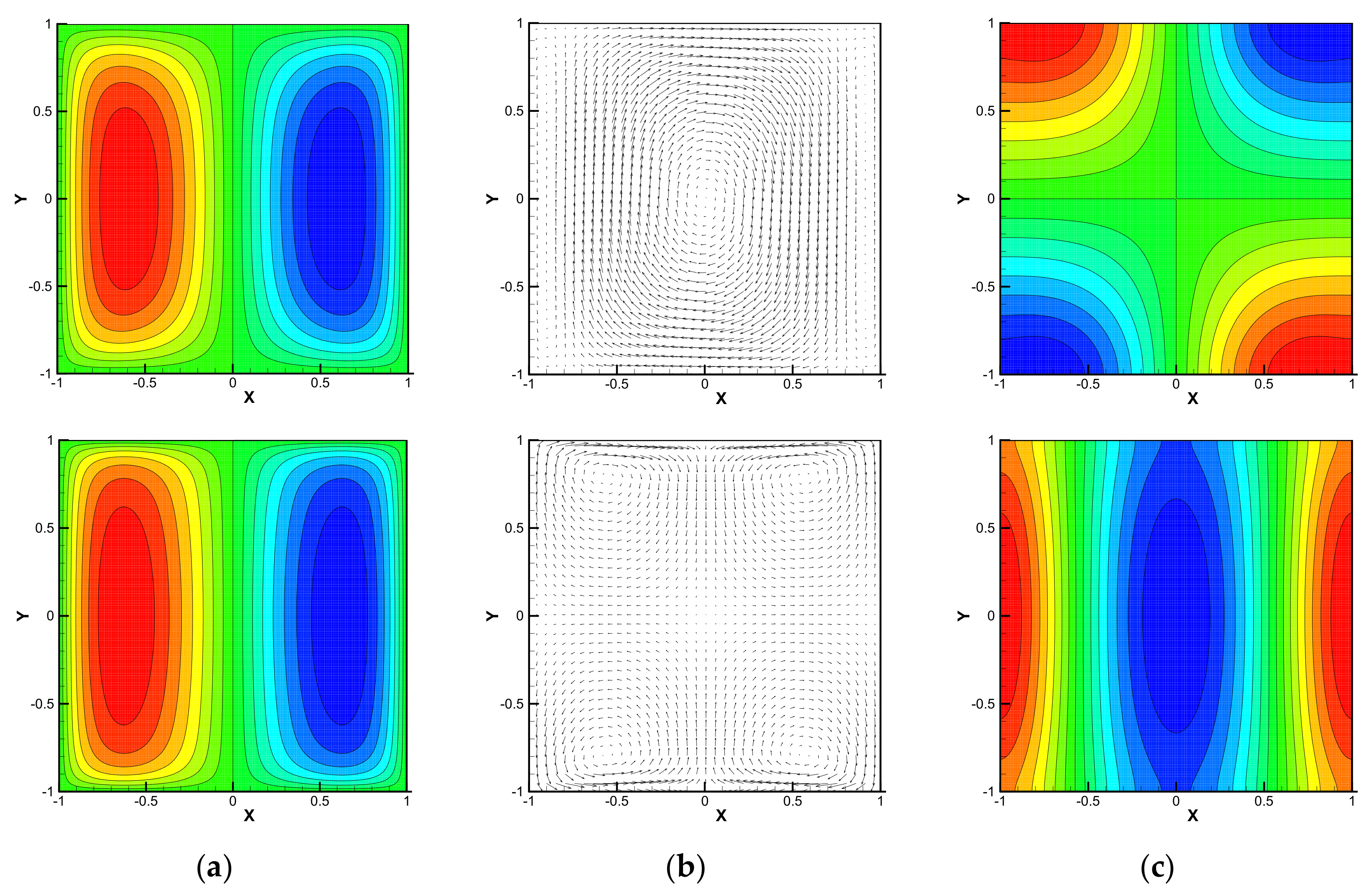
Figure 2 shows the velocity field, current density vectors, and electric potential in each basic state. The upper figures show the case where a magnetic field is applied in the X-direction at Ha = 2, and the lower figures show the case where a magnetic field is applied in the Y direction at Ha = 10. The basic state depends only on the magnetic field direction and the Hartmann number. It is independent of the Prandtl number and the Grashof number. When a magnetic field is applied in the X-direction, the Hartmann boundary layer is formed near the hot (left) and cold (right) walls, but as shown in the upper figure of Figure 2b, the current density generated in the core region does not need to pass through the Hartmann boundary layer, so there is no phenomenon that the current density concentrates in the Hartmann boundary layer. On the contrary, when a magnetic field is applied in the Y-direction, it is recognized that the current density is localized in the vicinity of the adiabatic walls because the current density generated in the core region must pass through the Hartmann boundary layer. Whether a magnetic field is applied in the X-direction or the Y-direction, the basic velocity, current density, and electric potential have symmetry with respect to the coordinate origin.

4. Linear Stability Analyses

4.1. Linearized Disturbance Equations

Next, the neutral unstable state of the basic state is investigated. First, it is assumed that each variable is given as the sum of the basic state and the infinitesimal disturbance.

$$\left(\begin{array}{l}{U}_i\\ \Theta \\ P\\ J_i\\ \Phi \end{array}\right)=\left(\begin{array}{l}{\overline{U}}_i\left(X,Y\right)\\ \overline{\Theta }\left(X,Y\right)\\ \overline{P}\left(X,Y\right)\\ {\overline{J}}_i\left(X,Y\right)\\ \overline{\Phi }\left(X,Y\right)\end{array}\right)+\left(\begin{array}{l}{U_i}^{\prime }\left(X,Y,Z,\tau \right)\\ {\Theta }^{\prime }\left(X,Y,Z,\tau \right)\\ P^{\prime }\left(X,Y,Z,\tau \right)\\ {J_i}^{\prime }\left(X,Y,Z,\tau \right)\\ {\Phi }^{\prime }\left(X,Y,Z,\tau \right)\end{array}\right).$$

(13)

Furthermore, it is considered that infinitesimal disturbance has a sinusoidal periodicity in the vertical direction.

$$\frac{{U_i}^{\prime }}{{\tilde{U}}_i\left(X,Y\right)}=\frac{{\Theta }^{\prime }}{\tilde{\Theta }\left(X,Y\right)}=\frac{P^{\prime }}{\tilde{P}\left(X,Y\right)}=\frac{{J_i}^{\prime }}{{\tilde{J}}_i\left(X,Y\right)}=\frac{{\Phi }^{\prime }}{\tilde{\Phi }\left(X,Y\right)}=\exp \left(ikZ+S\tau \right).$$

(14)

Ignoring the product of the quadratic disturbances appearing in the inertial term, finally, the following linearized equations can be obtained.

$$\frac{\partial \tilde{U}}{\partial X}+\frac{\partial \tilde{V}}{\partial Y}+ik\tilde{W}=0$$

(15)

$$S\tilde{U}+i\overline{W}k\tilde{U}=-\frac{\partial \tilde{P}}{\partial X}+\frac{1}{Gr}\left(\frac{{\partial }^2}{\partial X^2}+\frac{{\partial }^2}{\partial Y^2}-k^2\right)\tilde{U}+\frac{H{a}^2}{Gr}\left(-{\tilde{J}}_Z{B}_Y\right)$$

(16)

$$S\tilde{V}+i\overline{W}k\tilde{V}=-\frac{\partial \tilde{P}}{\partial Y}+\frac{1}{Gr}\left(\frac{{\partial }^2}{\partial X^2}+\frac{{\partial }^2}{\partial Y^2}-k^2\right)\tilde{V}+\frac{H{a}^2}{Gr}\left({\tilde{J}}_Z{B}_X\right)$$

(17)

$$\begin{array}{l}S\tilde{W}+\tilde{U}\frac{\partial \overline{W}}{\partial X}+\tilde{V}\frac{\partial \overline{W}}{\partial Y}+i\overline{W}k\tilde{W}\\ \hspace{1em}=-ik\tilde{P}+\frac{1}{Gr}\left(\frac{{\partial }^2}{\partial X^2}+\frac{{\partial }^2}{\partial Y^2}-k^2\right)\tilde{W}+\frac{1}{Gr}\tilde{\Theta }+\frac{H{a}^2}{Gr}\left({\tilde{J}}_X{B}_Y-{\tilde{J}}_Y{B}_X\right)\end{array}$$

(18)

$$S\tilde{\Theta }+i\overline{W}k\tilde{\Theta }=\tilde{U}+\frac{1}{GrPr}\left(\frac{{\partial }^2}{\partial X^2}+\frac{{\partial }^2}{\partial Y^2}-k^2\right)\tilde{\Theta }$$

(19)

$$\frac{\partial {\tilde{J}}_X}{\partial X}+\frac{\partial {\tilde{J}}_Y}{\partial Y}+ik{\tilde{J}}_Z=0$$

(20)

$${\tilde{J}}_X=-\frac{\partial \tilde{\Phi }}{\partial X}-\tilde{W}{B}_Y,\hspace{1em}{\tilde{J}}_Y=-\frac{\partial \tilde{\Phi }}{\partial Y}+\tilde{W}{B}_X,\hspace{1em}{\tilde{J}}_Z=-ik\tilde{\Phi }+\tilde{U}{B}_Y-\tilde{V}{B}_X.$$

(21)

Boundary conditions:

$$\left\{\begin{array}{l}X=\pm 1:\hspace{1em}\tilde{U}=\tilde{V}=\tilde{W}=0,\hspace{1em}\tilde{\Theta }=0,\hspace{1em}{\tilde{J}}_X=0\\ Y=\pm 1:\hspace{1em}\tilde{U}=\tilde{V}=\tilde{W}=0,\hspace{1em}\frac{d\tilde{\Theta }}{dY}=0,\hspace{1em}{\tilde{J}}_Y=0\end{array}\right.,$$

(22)

where S is a complex number, and it is the eigenvalue of these simultaneous linearized disturbance equations.

4.2. Numerical Methodology

Equations (15)–(22) are divided into a real part and an imaginary part, and spatial two-dimensional iterative computation is performed by using the fourth-order center difference method. Meanwhile, the pressure field (potential field) is obtained with modifying the velocity field (current density field) by the HSMAC (Highly-Simplified Marker And Cell) method so as to satisfy the continuity equation (conservation of electric charge). In addition, normalization is performed to prevent overflow or underflow of the value of each variable. The computational conditions are the direction of the applied magnetic field, the Hartmann number (Ha), the Prandtl number (Pr), the Grashof number (Gr), and the wavenumber (k) in the vertical direction. The corresponding eigenfunctions (velocity components, pressure, temperature, etc.) must be obtained. Newton’s method is applied to obtain the real part S_R and the imaginary part S_I of the eigenvalue S. The two values can be obtained by applying it to one of Equations (16)–(19). The following explanation is the case where Equation (16) is applied. It is divided into a real part and an imaginary part and is regarded as a function of only S_R and S_I, respectively.

$$\begin{array}{l}f\left(S_R\right)=-\left(S_R{\tilde{U}}_R-S_I{\tilde{U}}_I\right)+\overline{W}k{\tilde{U}}_I-\frac{\partial {\tilde{P}}_R}{\partial X}+\frac{1}{Gr}\left(\frac{{\partial }^2}{\partial X^2}+\frac{{\partial }^2}{\partial Y^2}-k^2\right){\tilde{U}}_R-\frac{H{a}^2}{Gr}\left({\tilde{J}}_{ZR}{B}_Y\right)\simeq 0\\ f\left(S_I\right)=-\left(S_R{\tilde{U}}_I+S_I{\tilde{U}}_R\right)-\overline{W}k{\tilde{U}}_R-\frac{\partial {\tilde{P}}_I}{\partial X}+\frac{1}{Gr}\left(\frac{{\partial }^2}{\partial X^2}+\frac{{\partial }^2}{\partial Y^2}-k^2\right){\tilde{U}}_I-\frac{H{a}^2}{Gr}\left({\tilde{J}}_{ZI}{B}_Y\right)\simeq 0\end{array}$$

(23)

From the formula of Newton’s method,

$$S_R{}^{n+1}=S_R{}^n-C_{1}f\left(S_R{}^n\right),\hspace{1em}{S}_I{}^{n+1}=S_I{}^n-C_{2}f\left(S_I{}^n\right),$$

(24)

where the superscript n represents the number of iterative steps and C₁ and C₂ are constants for adjusting the convergence speed of Newton’s method. By imposing Equation (24) at an arbitrarily selected grid point during the iterative calculation, the linear growth rate S_R and the angular frequency S_I can be simultaneously obtained.

The real part S_R of the eigenvalue obtained is not always zero (and the imaginary part S_I is not always zero either). For the purpose of drawing a neutral stability curve, one may want to find a combination of Pr, Ha, Gr, k, and S_I such that S_R becomes zero. Therefore, Pr, Ha, and k should be fixed first, while Gr is allowed to be slightly shifted from the preobtained solution, so that S_R becomes zero. At this time, S_I is also modified to some extent. Newton’s method can also be applied to the iterative correction. For example, using the growth rate S_R, it is given as follows.

$$G{r}^{n+1}=G{r}^n-C_3{S}_R{}^n,$$

(25)

where, C₃ is a positive constant for adjusting the convergence speed of Newton’s method. When the growth rate S_R is positive, it means that Gr is decreased. This is effective in finding the lower branch in the neutral stability curve. As can be seen from Equation (25), when S_R approaches zero, the value of Gr does not change and it converges. In this way, a neutral Grashof number can be obtained. On the other hand, in order to find the upper branch, the sign of the constant should be inverted. In the region connecting the upper branch and the lower branch, the gradient of the curve with respect to k is large, so it is more efficient to fix Gr and find k in the neutral stable state in order to keep computational accuracy. The more detailed numerical method on the linear stability analysis can be found in the recent paper [33].

4.3. Verification of the Code Developed

The main purpose of this study is to quantitatively capture the instability of MHD natural convection. In order to verify the validity of the developed code, the author first ignores the change in the Y-directional coordinate without considering the effect of magnetic field. The instability of natural convection in a vertical slot is taken up as a subject. Regarding this, it is known in previous studies that it exhibits a standing wave mode or a traveling wave mode depending on the value of the Prandtl number. The author first verifies the validity of the code in each case.

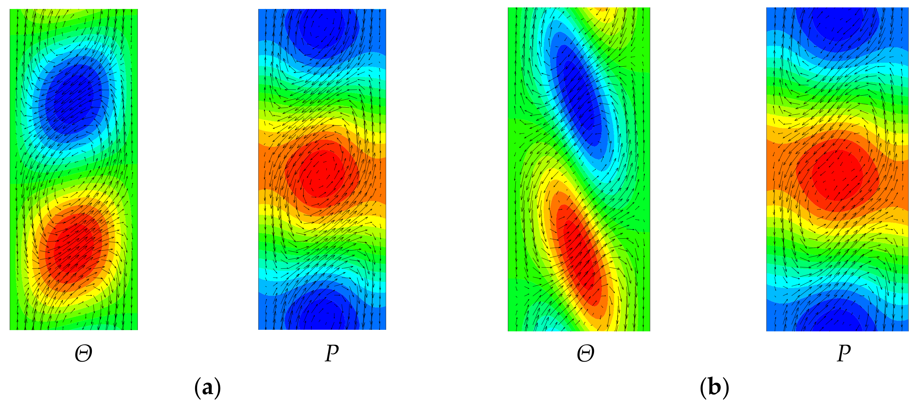
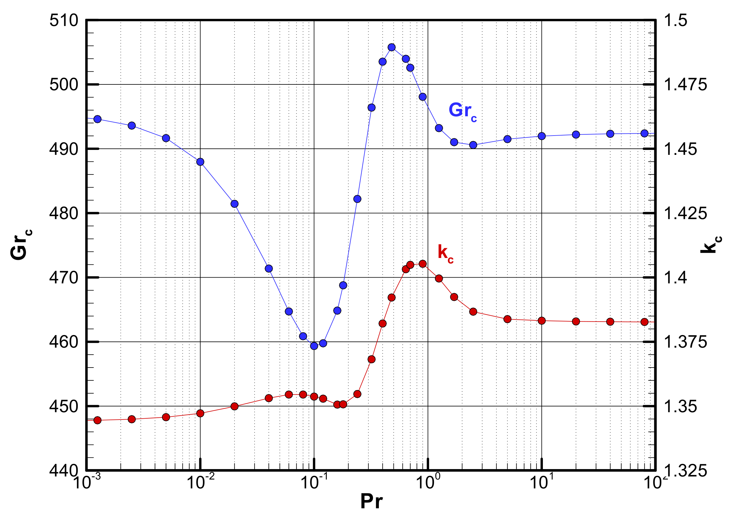
First, the results in the case of standing wave disturbance are shown. When computed with 201 grids for Pr = 0.01 and 0.7, the obtained critical wavenumber and critical Grashof number were k_c = 1.347 and Gr_c = 487.97 and k_c = 1.405 and Gr_c = 502.59, respectively. Figure 3 shows the visualization of the velocity and temperature under such conditions. Since periodicity is assumed in the vertical direction, only about one wave length is shown here. Convection cells (vortices) rotate in different directions between adjacent vortices, as observed in Bénard convection. However, the convection cell is not like a rectangle, but rather a shape close to a parallelogram. A clockwise vortex has the effect of strengthening the basic flow, so the pressure drops, while a counterclockwise vortex weakens the basic flow, so the pressure rises. It can be seen that the temperature is high in the flow part that separates from the heating surface on the left side, and the temperature is low in the flow part that separates from the cooling surface on the right side. Even if the Prandtl number is changed, the value of the critical Grashof number does not vary significantly as shown in Figure 4. This result was obtained with the number of grids 201 using the discretization of a fourth-order central difference method.

Next, the case of travelling wave mode is shown. The number of grids was tested with 101. Figure 5a shows the dependence of the dimensionless linear growth rate S_R and the angular frequency S_I on the wavenumber for Pr = 15 and Gr = 400. Since the angular frequency increases almost linearly, it can be seen that the phase velocity of the wave hardly depends on the wavenumber. Figure 5b shows the visualization of the travelling wave mode for k = 0.5. The temperature of the higher and lower parts near the right cold wall moves downward at a constant phase velocity.

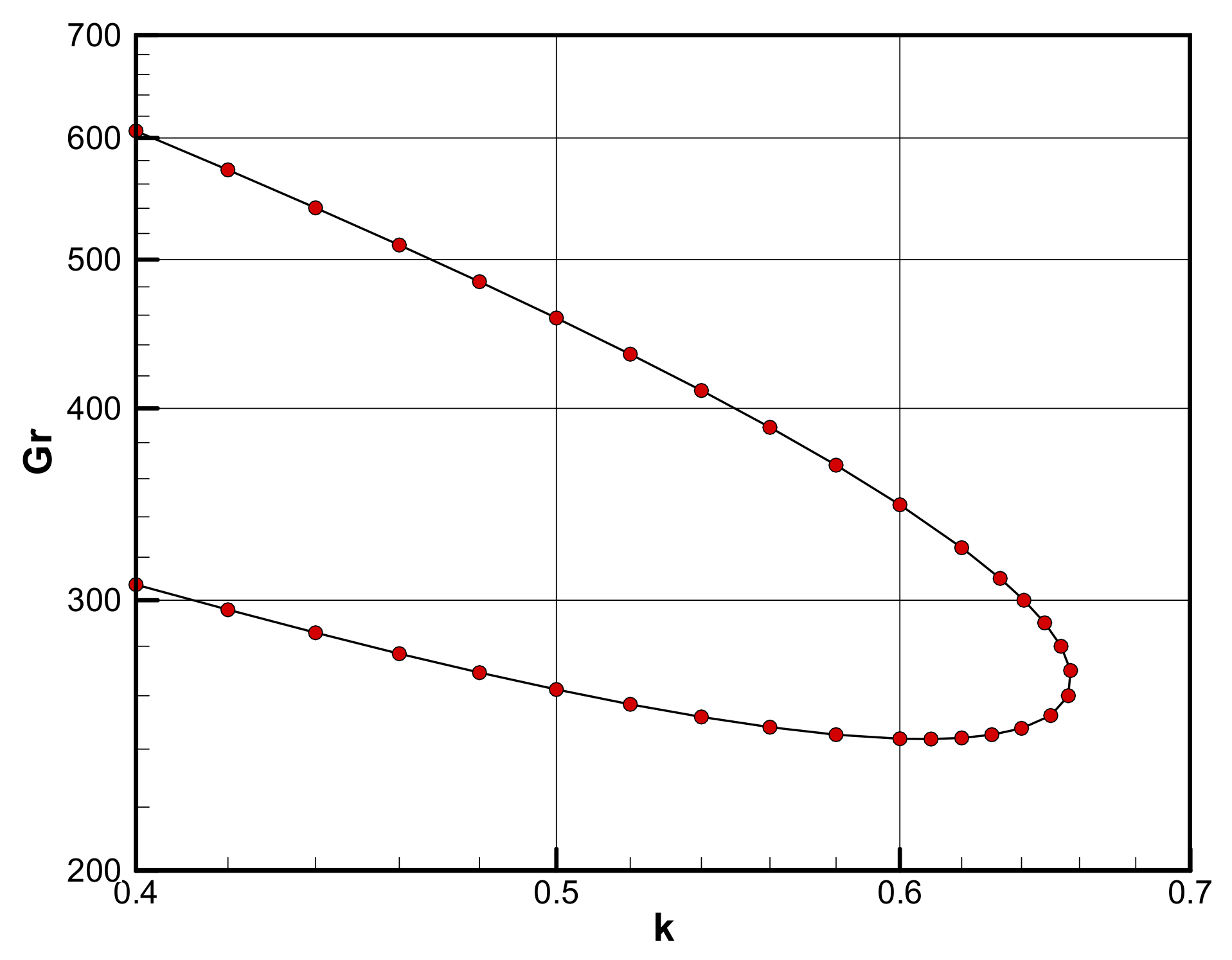
Figure 6 shows the neutral stability curve for Pr = 15. According to the method of the present computation and the number of grid points with 101, the critical Grashof number was about 243.6 and the critical wavenumber was 0.608. It can be seen that this critical Grashof number is lower than that of the standing wave mode.

4.4. Results for MHD Natural Convection

Judging from some numerical results obtained in the previous section and comparison with previous studies, the present numerical method is considered to be appropriate. In this section, the author describes the numerical results when a magnetic field is applied, with considering the change in the Y-direction. The Prandtl number of liquid metal is as small as about 0.025, and the author limits it to this value thereafter. Notice that as a result of various analyses, the angular frequency S_I always converged to zero, that is, the traveling wave mode did not appear in this study.

Table 1. The critical wavenumbers and Grashof numbers obtained for various Hartmann numbers with the mesh systems of 50 × 50 and 100 × 100 at Pr = 0.025.

Ha (Direction)	kc (50 × 50)	Grc (50 × 50)	Grn (100 × 100)
0	0.7085	2501.77	2497.79
0.1 (X)	0.7082	2506.12	2502.12
0.5 (X)	0.6986	2612.84	2608.45
1.0 (X)	0.6689	2977.45	2971.56
1.5 (X)	0.6207	3708.12	3698.37
2.0 (X)	0.5566	5072.35	5052.06
2.5 (X)	0.4838	7705.94	7650.83
3.0 (X)	0.4172	13,193.0	12,989.7
3.5 (X)	0.3562	26,057.7	25,019.8
4.0 (X)	0.3485	57,759.7	52,146.2
1 (Y)	0.7212	2442.15	2438.47
2 (Y)	0.7524	2310.72	2307.64
3 (Y)	0.7887	2189.21	2186.67
4 (Y)	0.8198	2124.65	2122.49
5 (Y)	0.8413	2129.52	2127.56
7 (Y)	0.8548	2338.08	2336.37
10 (Y)	0.8196	3121.67	3121.36
15 (Y)	0.6904	6149.12	6180.34
20 (Y)	0.5687	14,081.9	14,435.9
25 (Y)	0.4987	36,162.0	38,663.4

shows the results of the present computations. The Prandtl number was set to 0.025, assuming a typical liquid metal such as mercury or gallium. Ha represents the Hartmann number, X or Y represents the magnetic field direction, and k represents the critical wavenumber obtained by the computation of the coarser grid system (50 × 50). When a magnetic field is applied in the X-direction, the critical Grashof number for the onset of instability increases monotonically as increase in the Hartmann number. On the other hand, when a magnetic field is applied in the Y-direction, the critical Grashof number tends to decrease once at about Ha = 4, and then the Grashof number tends to increase as the magnetic field is further increased. The critical Grashof number tends to vary greatly depending on the direction of the magnetic field. It can also be seen that when the Hartmann number is large, the dependency of the number of grids is large. In the Y-directional magnetic field, the critical Grashof number tends to increase as the number of grids increases, but in the X-directional magnetic field, the opposite tendency is observed.

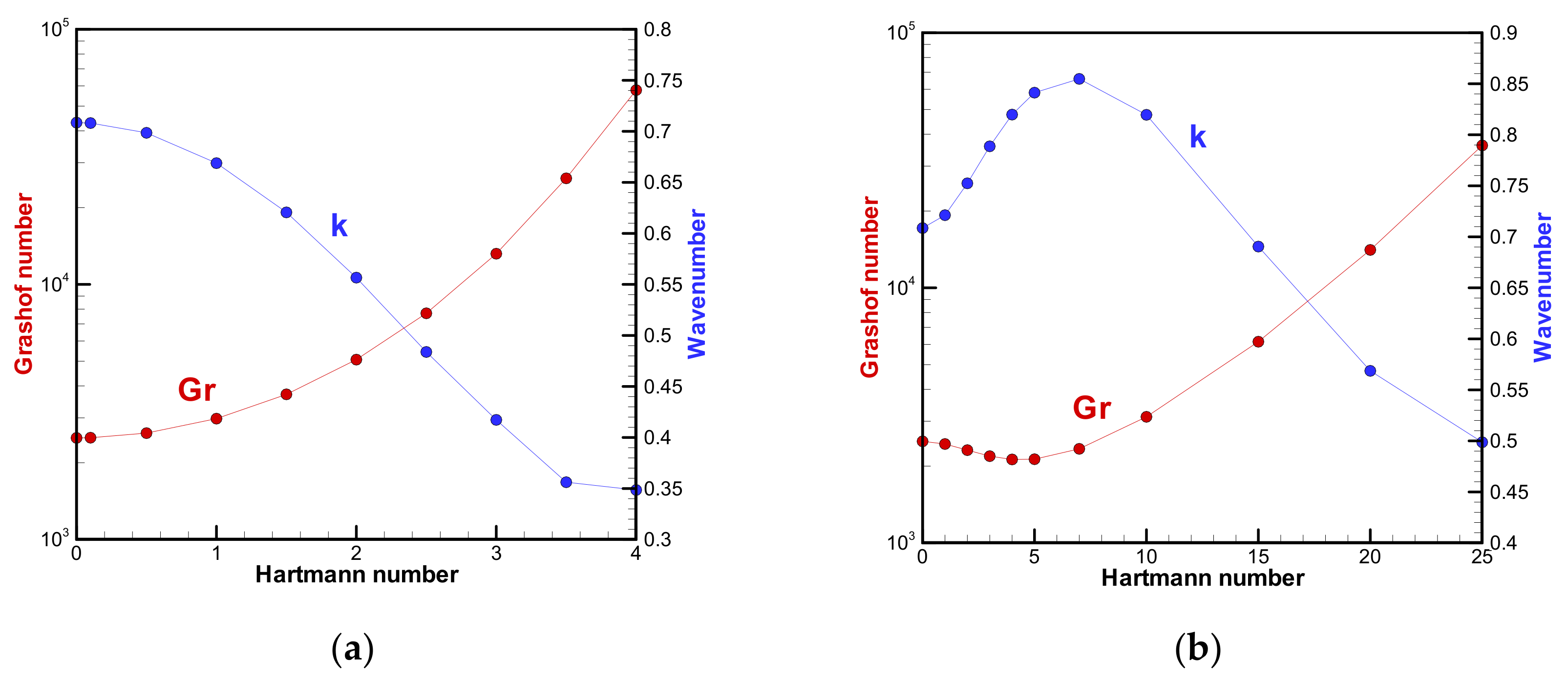
Figure 7 shows the results in Table 1 graphically for each magnetic field direction. The red line indicates the Grashof number and the blue line is the axial wavenumber. It can be seen that the X-directional magnetic field is much more stable than the Y-directional magnetic field. In the case of the Y-directional magnetic field, it can be seen that not only the critical Grashof number takes its minimum at a certain value of the Hartmann number but the critical wavenumber also takes its maximum at another value of the Hartmann number.

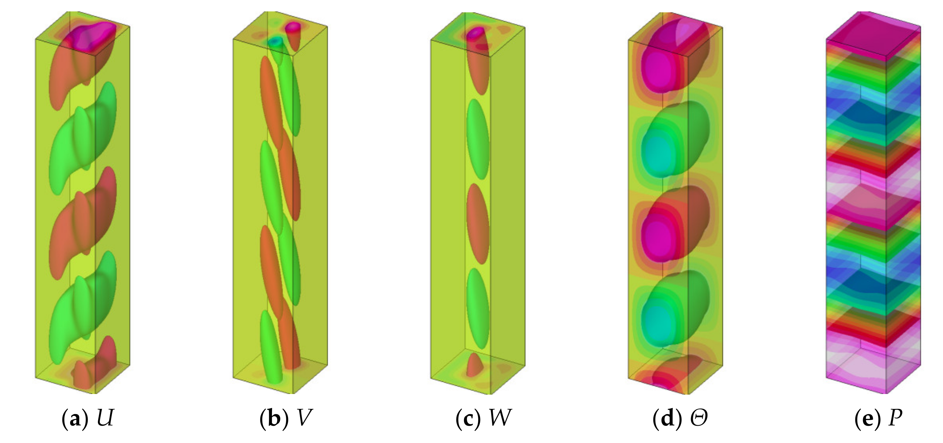
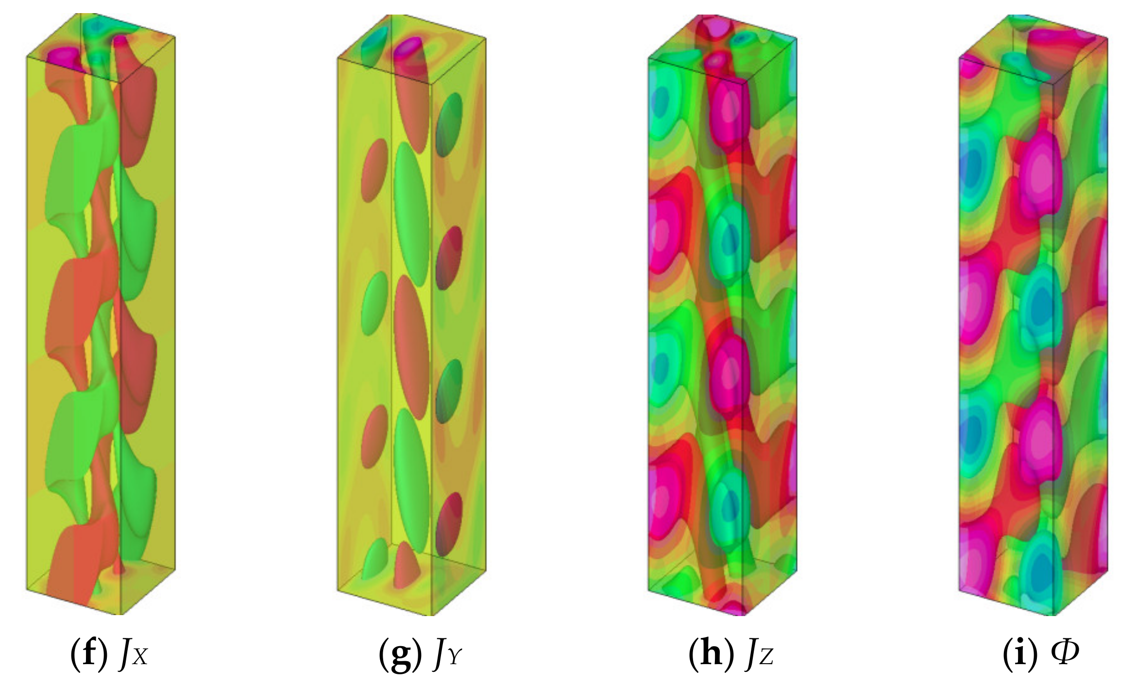
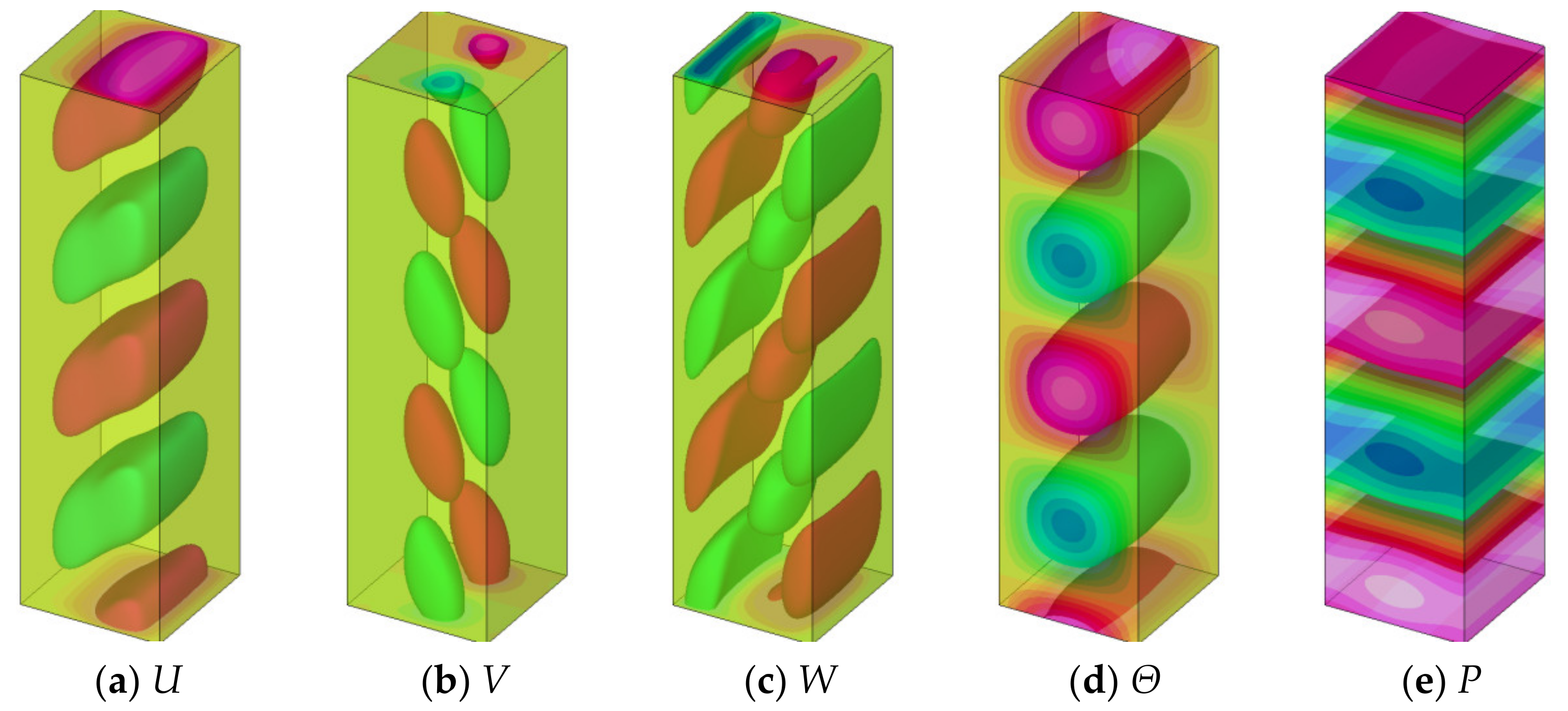
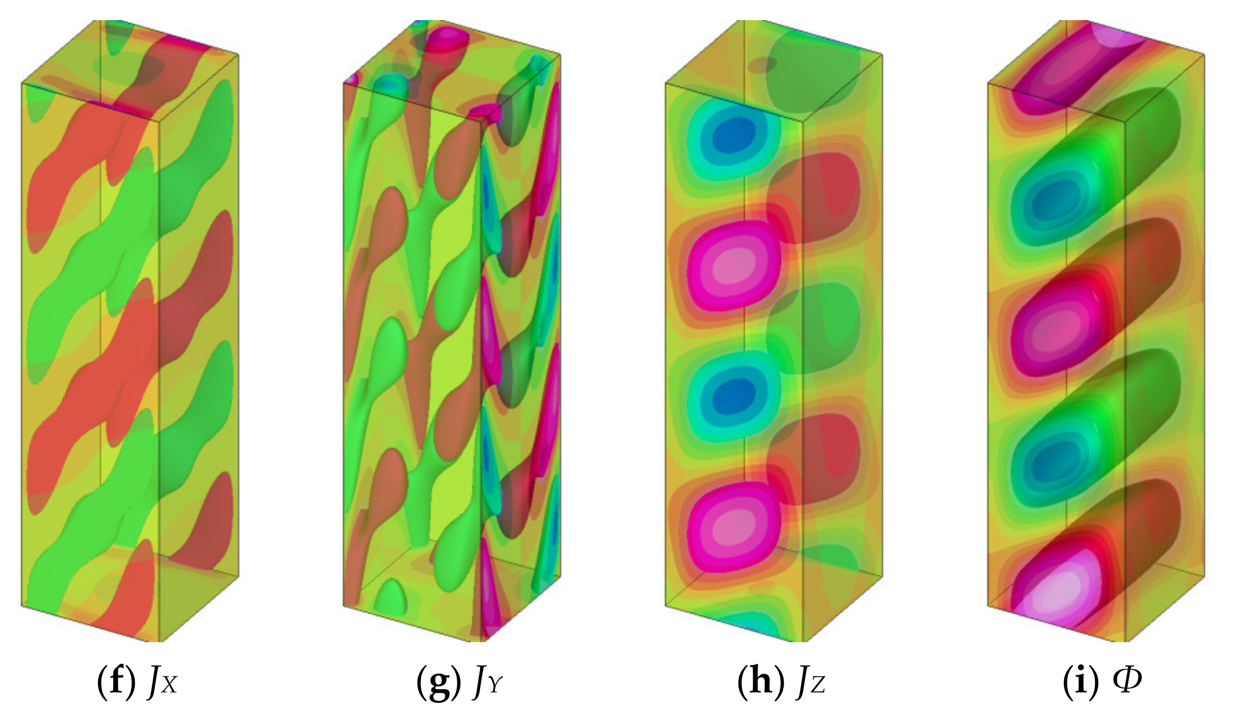
Figure 8 shows the visualization of the critical mode where a magnetic field is applied in the X-direction. The range of this three-dimensional visualization is for two wavelengths, but it is compressed in half in the vertical direction to save space. The vertical surface on the left side corresponds to the hot wall, and the vertical surface on the right side corresponds to the cold wall. (a) represents the velocity component in the X-direction, and the positive part is displayed in red and the negative part is displayed in green. This flow causes high and low temperature distributions, as seen in (d). In this case, since a weak magnetic field of Ha = 2 is applied, no large deformation is seen in the basic flow as shown in Figure 2. The velocity field, temperature field, and pressure field of (a), (b), (c), (d), and (e) are not much different from those in Figure 9. However, the current density and potential distributions of (f), (g), (h), and (i) are very different.

Figure 9 shows visualization diagrams when a magnetic field is applied in the Y-direction. The container does not look slender compared to that of X-directional magnetic field because the wavenumber is relatively large. It is compressed and visualized in half in the vertical direction. When a uniform magnetic field is applied in the Y-direction, a quasi-two-dimensional flow field with little change in the magnetic field direction is formed. In that case, it is known that the potential distribution in (i) is close to the stream function distribution. That is, it is almost allowed to consider that the flow is generated along the iso-surface of this potential. The green part of the potential shows a clockwise vortex, and the red part shows a counterclockwise vortex. The pressure in (e) becomes low in the clockwise part and high in the counterclockwise part because the vortex is weakened or strengthened when the fluctuation amount of the flow overlaps with the basic flow. This is the reason why the pressure is low in the forward-rotating vortex and high in the counter-rotating vortex. The strong current density appears in the vicinity of the vertical wall perpendicular to the magnetic field, as can be judged from (f) and (h). This is called the Hartmann boundary layer, and it has a boundary layer thickness that is roughly proportional to the inverse of the Hartmann number. The current density is concentrated inside the Hartmann boundary layer because all the current generated in the core region must pass through this Hartmann boundary layer.

5. Discussion

So far, the author has shown the effects of the X-directional magnetic field and the Y-directional magnetic field on the flow instability. It was found that the X-directional magnetic field is effective in stabilizing the flow when its strength increases, whereas the Y-directional magnetic field destabilizes the flow once, but it can stabilize the flow when the magnetic field strength increases. In both magnetic fields, the flow and electric potential fields in the basic state have two-fold line symmetry. Here, the author would like to discuss the stability of the flow when the symmetry of the basic state is slightly distorted. In other words, the author verifies the case where the uniform horizontal magnetic field is applied obliquely and investigates the symmetry breaking of the basic state and the corresponding critical Grashof number. When the angle between the magnetic field direction and the X-axis is defined as θ as seen in Figure 1b, θ = 0° corresponds to the X-directional magnetic field, and θ = 90° corresponds to the Y-directional magnetic field. As an example, the author demonstrated the numerical calculations performed in 15° increments for Ha = 3.

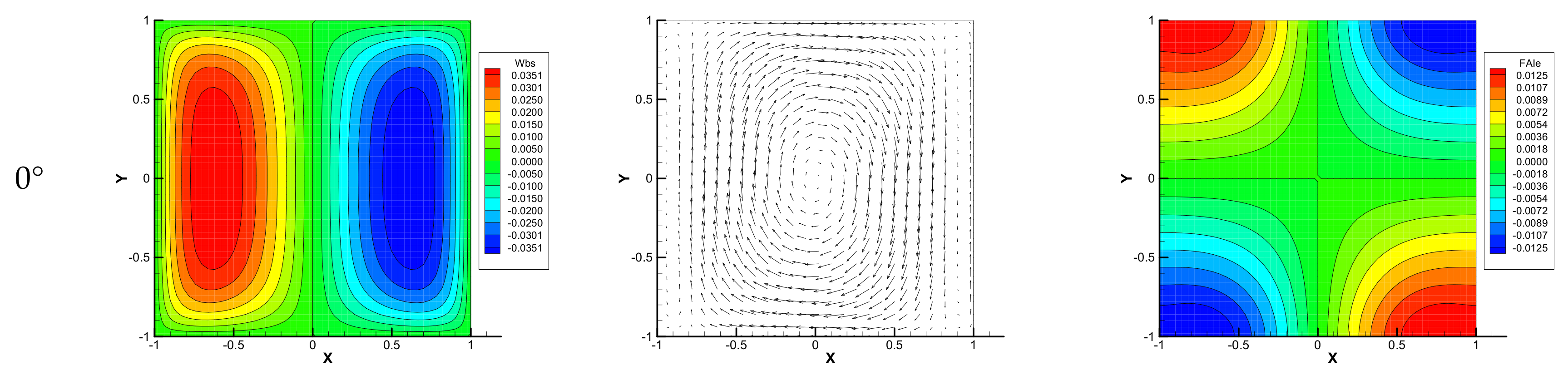
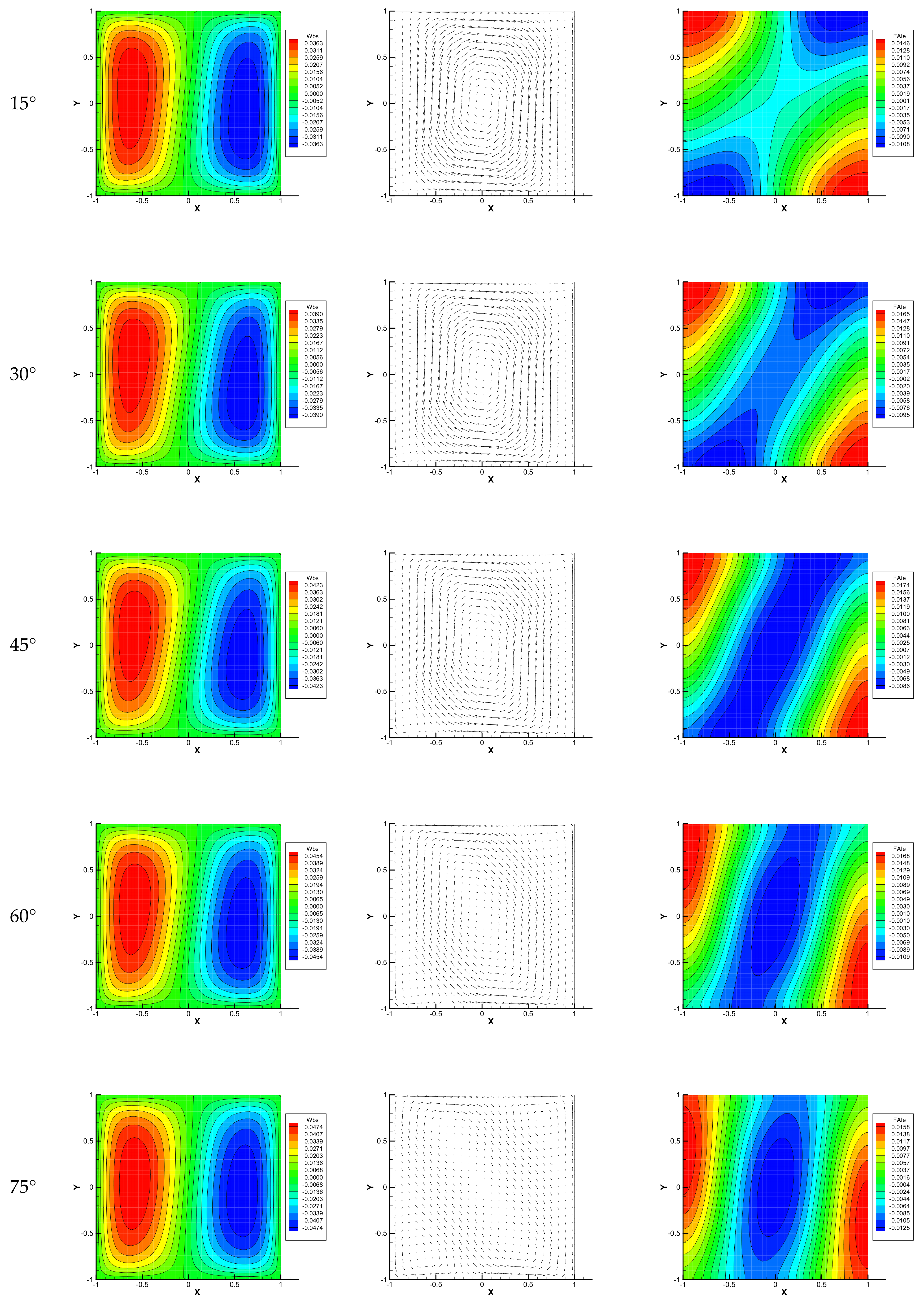
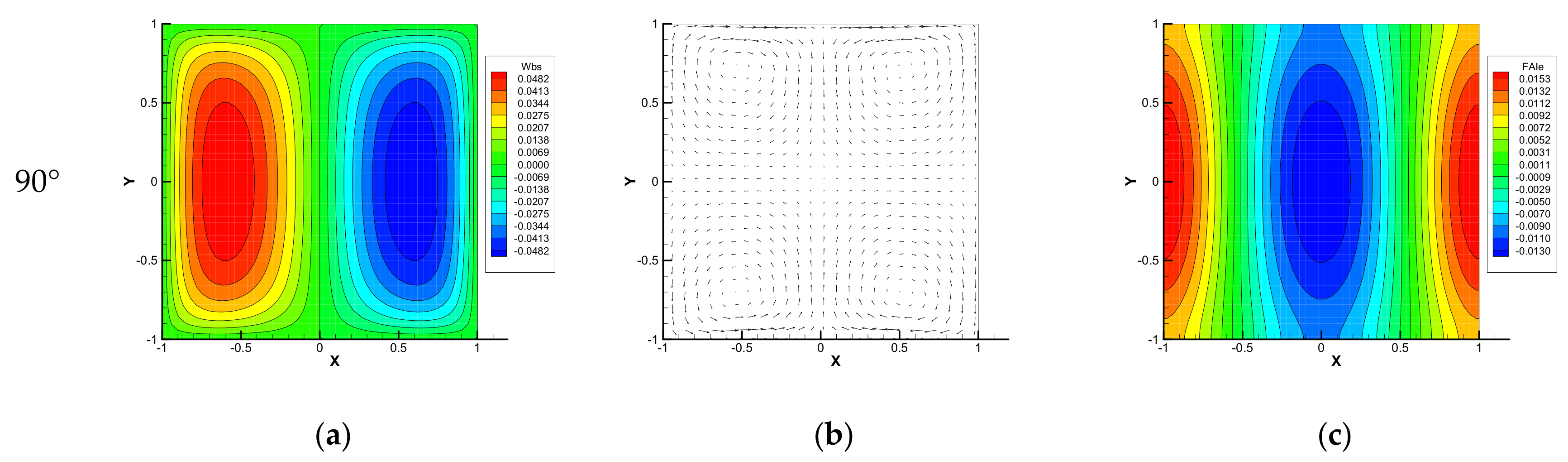
Figure 10 shows a horizontal cross-sectional view of the basic state (vertical velocity, current density vector, and electric potential) when a magnetic field is applied obliquely (in 15° increments). It can be recognized that the vertical velocity and electric potential maintain two-fold line symmetry at 0° and 90°, while they have only point symmetry at other magnetic field angles. It can be seen that the velocity value increases monotonically as the magnetic field angle increases. This suggests that the magnetic damping effect for the basic flow depends on the magnetic field angle. As the magnetic field angle increases, the current density gradually changes in its structure from a large clockwise vortex to four vortices. Note that all the seven have the same standard of drawing vectors.

Table 2. The effect of the angle of the magnetic field on the critical wavenumber and Grashof number at Pr = 0.025 and Ha = 3 when the mesh system of 50 × 50 was employed.

Angle, θ rad	kc	Grc
0 (X-mag.)	0.4172	13,193
π/12	0.4424	11,964
π/6	0.5155	8240.4
π/4	0.6082	4813.4
π/3	0.7015	3112.7
5π/12	0.7662	2389.4
π (Y-mag.)	0.7887	2189.2

shows the critical wavenumber and the Grashof number for each basic flow shown in Figure 10. The number of grids for the computations is the same as those for the basic flow, which is 50 × 50. It can be seen that the value of the critical wavenumber increases monotonically as the magnetic field angle increases. On the other hand, the value of the critical Grashof number decreases as the magnetic field angle increases. Note that even at 75°, the critical Grashof number is lower than in the case of no magnetic field.

6. Conclusions

In this paper, the author examined the linear stability of natural convection in a vertically long rectangular container under a uniform horizontal magnetic field. The following is a summary of this study. When the X-directional magnetic field is applied, the flow is stabilized monotonically as the Hartmann number increases. When the Y-directional magnetic field is applied, the flow becomes more unstable once with a weak magnetic field, and then it stabilizes as it becomes stronger. When an oblique magnetic field is applied, its damping effect on the basic flow and the critical Grashof number take the intermediate value between those of the X- and Y-directional magnetic fields.

References

- Moreau, R.J. Fluid Mechanics and Its Application. In Magnetohydrodynamics; Kluwer Academic Publishers: Dordrecht, The Netherlands; Norwell, MA, USA, 1990; Volume 3. [Google Scholar]
- Molokov, S.; Moreau, R.; Moffatt, H.K. Fluid Mechanics and Its Application. In Magnetohydrodynamics: Historical Evolution and Trends; Springer: Berlin/Heidelberg, Germany, 2007; Volume 80. [Google Scholar]
- Ozoe, H. Magnetic Convection; Imperial College Press: London, UK, 2005. [Google Scholar]
- Chandrasekhar, S. Hydrodynamic and Hydromagnetic Stability; Dover Publication: Mineola, NY, USA, 1961. [Google Scholar]
- Burr, U.; Müller, U. Rayleigh–Bénard convection in liquid metal layers under the influence of a vertical magnetic field. Phys. Fluids 2001, 13, 3247–3257. [Google Scholar] [CrossRef]
- Burr, U.; Müller, U. Rayleigh-Bénard convection in liquid metal layers under the influence of a horizontal magnetic field. J. Fluid Mech. 2002, 453, 345. [Google Scholar] [CrossRef]
- Mistrangelo, C.; Bühler, L. Magneto-convective instabilities in horizontal cavities. Phys. Fluids 2016, 28, 024104. [Google Scholar] [CrossRef]
- Vest, C.M.; Arpaci, V.S. Stability of natural convection in a vertical slot. J. Fluid Mech. 1969, 36, 1–15. [Google Scholar] [CrossRef]
- Hart, J.E. Stability of the flow in a differentially heated inclined box. J. Fluid Mech. 1971, 47, 547–576. [Google Scholar] [CrossRef]
- Bergholz, R.F. Instability of steady natural convection in a vertical fluid layer. J. Fluid Mech. 1978, 84, 743–768. [Google Scholar] [CrossRef]
- Choi, I.; Korpela, S.A. Stability of the conduction regime of natural convection in a tall vertical annulus. J. Fluid Mech. 1980, 99, 725–738. [Google Scholar] [CrossRef]
- Lee, Y.; Korpela, S. Multicellular natural convection in a vertical slot. J. Fluid Mech. 1983, 126, 91–121. [Google Scholar] [CrossRef]
- Chen, Y.M.; Pearlstein, A.J. Stability of free-convection flows of variable-viscosity fluids in vertical and inclined slots. J. Fluid Mech. 1989, 198, 513–541. [Google Scholar] [CrossRef]
- Fujimura, K.; Mizushima, J. Nonlinear equilibrium solutions for travelling waves in a free convection between vertical parallel plates. Eur. J. Mech. B Fluids 1991, 10, 25–30. [Google Scholar]
- McAllister, A.; Steinolfson, R.; Tajima, T. Vertical Slot Convection: A Linear Study (No. DOE/ET/53088-584; IFSR--584); Institute for Fusion Studies, Texas University: Austin, TX, USA, 1992. [Google Scholar]
- Lartigue, B.; Lorente, S.; Bourret, B. Multicellular natural convection in a high aspect ratio cavity: Experimental and numerical results. Int. J. Heat Mass Transf. 2000, 43, 3157–3170. [Google Scholar] [CrossRef]
- Bratsun, D.A.; Zyuzgin, A.V.; Putin, G.F. Non-linear dynamics and pattern formation in a vertical fluid layer heated from the side. Int. J. Heat Fluid Flow 2003, 24, 835–852. [Google Scholar] [CrossRef]
- Wright, J.L.; Jin, H.; Hollands, K.G.T.; Naylor, D. Flow visualization of natural convection in a tall, air-filled vertical cavity. Int. J. Heat Mass Transf. 2006, 49, 889–904. [Google Scholar] [CrossRef] [Green Version]
- Ganguli, A.A.; Pandit, A.B.; Joshi, J.B. Numerical predictions of flow patterns due to natural convection in a vertical slot. Chem. Eng. Sci. 2007, 62, 4479–4495. [Google Scholar] [CrossRef]
- Fogaing, M.T.; Nana, L.; Crumeyrolle, O.; Mutabazi, I. Wall effects on the stability of convection in an infinite vertical layer. Int. J. Therm. Sci. 2016, 100, 240–247. [Google Scholar] [CrossRef]
- Suslov, S.A.; Paolucci, S. Stability of natural convection flow in a tall vertical enclosure under non-Boussinesq conditions. Int. J. Heat Mass Transf. 1995, 38, 2143–2157. [Google Scholar] [CrossRef]
- Kitada, T.; Kato, Y.; Fujimura, K. Non-Boussinesq effects on the linear stability of thermal convection in an inclined slot. Trans. Jpn. Soc. Mech. Eng. Ser. B 2002, 68, 1002–1007. [Google Scholar] [CrossRef]
- Takashima, M. The stability of natural convection in a vertical layer of electrically conducting fluid in the presence of a transverse magnetic field. Fluid Dyn. Res. 1994, 14, 121. [Google Scholar] [CrossRef]
- Nagata, M. Nonlinear analysis on the natural convection between vertical plates in the presence of a horizontal magnetic field. Eur. J. Mech. B Fluids 1998, 17, 33–50. [Google Scholar] [CrossRef]
- Burr, U.; Barleon, L.; Jochmann, P.; Tsinober, A. Magnetohydrodynamic convection in a vertical slot with horizontal magnetic field. J. Fluid Mech. 2003, 475, 21. [Google Scholar] [CrossRef]
- Hudoba, A.; Molokov, S. Linear stability of buoyant convective flow in a vertical channel with internal heat sources and a transverse magnetic field. Phys. Fluids 2016, 28, 114103. [Google Scholar] [CrossRef] [Green Version]
- Wong, C.P.C.; Malang, S.; Sawan, M.; Dagher, M.; Smolentsev, S.; Merrill, B.; Youssef, M.; Reyes, S.; Sze, D.; Morley, N.; et al. An overview of dual coolant Pb–17Li breeder first wall and blanket concept development for the US ITER-TBM design. Fusion Eng. Des. 2006, 81, 461–467. [Google Scholar] [CrossRef] [Green Version]
- Soto, C.; Smolentsev, S.; García-Rosales, C. Mitigation of MHD phenomena in DCLL blankets by Flow Channel Inserts based on a SiC-sandwich material concept. Fusion Eng. Des. 2020, 151, 111381. [Google Scholar] [CrossRef]
- Tagawa, T.; Authié, G.; Moreau, R. Buoyant flow in long vertical enclosures in the presence of a strong horizontal magnetic field. Part 1. Fully-established flow. Eur. J. Mech. B Fluids 2002, 21, 383–398. [Google Scholar] [CrossRef]
- Authié, G.; Tagawa, T.; Moreau, R. Buoyant flow in long vertical enclosures in the presence of a strong horizontal magnetic field. Part 2. Finite enclosures. Eur. J. Mech. B Fluids 2003, 22, 203–220. [Google Scholar] [CrossRef]
- Lyubimov, D.V.; Lyubimova, T.P.; Perminov, A.B.; Henry, D.; Hadid, H.B. Stability of convection in a horizontal channel subjected to a longitudinal temperature gradient. Part 2. Effect of a magnetic field. J. Fluid Mech. 2009, 635, 297–319. [Google Scholar] [CrossRef] [Green Version]
- Kitaura, T.; Tagawa, T. Linear stability analysis of thermal convection in an infinitely long vertical rectangular enclosure in the presence of a uniform horizontal magnetic field. J. Fluids 2014, 2014, 642042. [Google Scholar] [CrossRef] [Green Version]
- Tagawa, T. Linear stability analysis of liquid metal flow in an insulating rectangular duct under external uniform magnetic field. Fluids 2019, 4, 177. [Google Scholar] [CrossRef] [Green Version]
Figure 1.
Geometrical configuration of the problem: (a) the rectangular enclosure is sufficiently long in the vertical direction. The basic temperature is in heat conduction state and the basic flow is assumed to have only vertical component of velocity. (b) A uniform horizontal magnetic field is applied in either the X-direction, the Y-direction, or the oblique direction.
Figure 2.
Basic states within a cross-section for the case of an infinitely long vertical enclosure. The upper ones indicate the case of X-directional magnetic field at Ha = 2, and the lower the case of Y-directional magnetic field at Ha = 10: (a) contour map of the vertical component of velocity, (b) electric current density vectors, and (c) contour map of the electric potential.
Figure 3.
Velocity vectors, temperature and pressure at the onset of instability: (a) Pr = 0.01, kc = 1.347 and Grc = 487.97; (b) Pr = 0.7, kc = 1.405 and Grc = 502.59.
Figure 4.
Variations of the critical Grashof number and the critical wavenumber for the wide range of the Prandtl number.
Figure 5.
(a) Linear growth rate SR and angular frequency SI as a function of wavenumber k at Pr = 15 and Gr = 400 and (b) contour map of temperature and velocity vectors (visualized by compressing twice in the vertical direction) at Pr = 15, Gr = 400, k = 0.5, SI = 0.0297, and SR = 1.06 × 10⁻⁴.
Figure 6.
Neutral stability curve between the Grashof number and wavenumber at Pr = 15.
Figure 7.
Effect of the Hartmann number on the critical Grashof number and the wavenumber at Pr = 0.025: (a) X-directional magnetic field and (b) Y-directional magnetic field.
Figure 8.
The mode at the onset of instability for the case of X-directional magnetic field at Pr = 0.025, Ha = 2, and k = 0.5566. Each figure is visualized by two isosurfaces as well as contour maps on the walls: (a) X-directional velocity, (b) Y-directional velocity, (c) Z-directional velocity, (d) temperature, (e) pressure, (f) X-directional current density, (g) Y-directional current density, (h) Z-directional current density, and (i) electric potential.
Figure 9.
The mode at the onset of instability for the case of Y-directional magnetic field at Pr = 0.025, Ha = 10, and k = 0.8196. Each figure is visualized by two isosurfaces as well as contour maps on the walls: (a) X-directional velocity, (b) Y-directional velocity, (c) Z-directional velocity, (d) temperature, (e) pressure, (f) X-directional current density, (g) Y-directional current density, (h) Z-directional current density, and (i) electric potential.
Figure 10.
Effect of the direction of the magnetic field on the basic state at Ha = 3: (a) vertical component of velocity, (b) electric current density vectors, and (c) electric potential.