Multi-Visual Feature Saliency Detection for Sea-Surface Targets through Improved Sea-Sky-Line Detection

1
Marine Engineering College and Key Laboratory of Fujian province Marine and Ocean Engineering, Jimei University, Xiamen 361021, China
2
School of Mechanical and Electrical Engineering, Putian University, Putian 351100, China
3
Key Laboratory of Modern Precision Measurement and Laser Nondestructive Detection Colleges and Universities in Fujian Province, Putian 351100, China
4
College of Merchant Marine, Shanghai Maritime University, Shanghai 201306, China
*
Author to whom correspondence should be addressed.
J. Mar. Sci. Eng. 2020, 8(10), 799; https://doi.org/10.3390/jmse8100799
Submission received: 3 October 2020
/
Revised: 10 October 2020
/
Accepted: 12 October 2020
/
Published: 15 October 2020
(This article belongs to the Special Issue Marine Measurements: Theory, Methods and Applications)
Abstract
:To visually detect sea-surface targets, the objects of interest must be effectively and rapidly isolated from the background of sea-surface images. In contrast to traditional image detection methods, which employ a single visual feature, this paper proposes a significance detection algorithm based on the fusion of multi-visual features after detecting the sea-sky-lines. The gradient edges of the sea-surface images are enhanced using a Gaussian low-pass filter to eliminate the effect of the image gradients pertaining to the clouds, wave points, and illumination. The potential region and points of the sea-sky-line are identified. The sea-sky-line is fitted through polynomial iterations to obtain a sea-surface image containing the target object. The saliency subgraphs of the high and low frequency, gradient texture, luminance, and color antagonism features are fused to obtain an integrated saliency map of the sea-surface image. The saliency target area of the sea surface is segmented. The effectiveness of the proposed method was verified. The average detection rate and time for the sea-sky-line detection were 96.3% and 1.05 fps, respectively. The proposed method outperformed the existing saliency models on the marine obstacle detection dataset and Singapore maritime dataset, with mean absolute errors of 0.075 and 0.051, respectively.
1. Introduction
With the development of computer vision technology, the role of cameras as an imaging technique is becoming increasingly more important, and cameras are being widely used in unmanned ships to provide reliable information to realize intelligent decision-making. The ocean images can be divided into three parts: sky, sea, and sea-sky-line. The sea-sky-line is a connecting line between the sky and the sea background. It is often visually formed by an outline of the sky and the gray scale of the sea and sky background. When an object appears in a camera’s field of view, it is usually near the sea-sky-line. With a decrease in the distance to the target, the target gradually appears to be within the sea surface. The range of target detection can be considerably reduced by extracting the sea-sky-line information and conducting offshore target detection near the sea-sky-lines. Moreover, the complexity and amount of computation in the algorithm can be reduced. Therefore, by detecting the sea-sky-lines, image segmentation can be realized. In this manner, different detection and tracking strategies can be applied to different regions, and the robustness of the detection method can be improved.
1.1. Sea-Sky-Line Detection
Sea-sky-lines can provide valuable reference information for the obstacle avoidance systems of unmanned surface vehicles (USVs), as the obstacles that threaten the safety of USVs, such as ships and rocks, are generally located below the level of the sea-sky-line. The existing methods detect sea-sky-lines using only gray, textural, or line features in an optical image. However, the background features in the images obtained by onboard cameras are complex and change continuously over time, which leads to the poor robustness of these methods [1,2,3,4].
The existing methods to detect sea-sky-lines usually involve the following steps. First, the image is pre-processed to reduce the image noise. Subsequently, the characteristics around the sea-sky-line are strengthened and extracted to determine the approximately location of the sea-sky-line. Finally, the location of the ocean skyline is determined using the threshold method or linear fitting method. To detect the position of sea-sky-lines, researchers have attempted to use the Hough transform [5,6], Random sample consensus (RANSAC) line fitting [7], Radon transform [8], and Canny methods [9]. However, these methods depend strongly on the background complexity and are thus easily affected by clouds, waves, and floating objects.
Wang et al. [5] proposed a sea-sky-line detection algorithm based on the gradient saliency and region growth. The gradient saliency calculation effectively improved the characteristics of the sea-sky-line and suppressed the influence of complex sea conditions such as clouds and sea clutter. Dai et al. [10] proposed an edge detection algorithm based on a local Otsu segmentation and Hough transform, which solved the problem of poor global threshold segmentation. In addition, researchers have attempted to use the information entropy and histograms [11] to strengthen the features of the region around the sea-sky-line. However, large ships on the sea may affect the gray value of the entire image, thereby affecting the results of histogram analysis methods. In addition, the computational complexity of the information entropy may not be able to be satisfied in real scenes. In addition, most of the sea-sky-line methods can only be applied to infrared images. Jian et al. [12] proposed a method based on gradient smoothing and bimodal histogram analyses to improve the robustness and accuracy of sea-sky-line detection. Recently, machine learning [13,14] has been applied to achieve satisfactory results in image processing tasks. However, to implement such methods, a large number of images must be collected in advance for training. Moreover, practical application scenarios involve unpredictable factors such as insufficient light intensity, inclement weather, presence of ships, and undulations on the sea surface, and the pre-trained model may not be able achieve satisfactory results under such conditions.
1.2. Saliency Detection
The visual attention mechanism of saliency detection is similar to that of the attention detection of the human eye, through which the visually “attention” region can be automatically extracted from an image or video. In recent work, saliency detection has been considered a specific task to be performed in a top-down manner by assuming the existence of prior knowledge or certain constraints regarding the scene [15]. Such task-driven approaches are particularly suited to realize the identification and retrieval of known objects, as such processes require knowledge learning or accumulation, which increase the complexity of the saliency detection. Consequently, visual attention mechanisms involving adaptable bottom-up algorithms are being widely examined.
Bottom-up saliency models can be classified as spatial [16,17] or spectral [18,19] models based on the domain extraction of the features. Itti et al. [20] obtained salient images by using the difference in the center-periphery of images, based on the color, intensity, and directional features of the images. Arya et al. [21] employed a double-density double-tree complex wavelet transform along with hyperpixel segmentation to realize saliency target detection. Chen et al. [22] used the spatial and time clues in the image as local constraints and developed a spatial constraint optimization model to realize video image saliency detection and global saliency optimization. Zhang et al. [23] established a saliency target detection model for a deep convolutional network and adopted a multi-scale fusion structure to obtain high-precision saliency target detection results. Wang [24] proposed a spatial-deep-learning significant target detection model for videos, which involved a full convolutional network to effectively detect the significant regions in video streams. Singh et al. [25] developed a model using a convolutional encoder–decoder to realize the significant target detection in noisy images. In general, in the case of spatial saliency models [26,27], the salient features of the objects can be effectively identified in simple scenes. However, such methods exhibit an inferior performance in complex scenes [28]. In other words, a single-image-related underlying feature cannot highlight the saliency objects in the image, and a linear combination of these features must be employed [29].
Overall, the aforementioned algorithms have achieved reasonable results in the corresponding research fields; however, it remains challenging to attain a high detection accuracy for sea-sky-lines and saliency detection in the case of complex backgrounds. To address these problems, in this work, considering the principle of bottom-up image saliency detection, a saliency detection algorithm employing multi-visual features of sea-surface images was developed, based on improved sea-sky-line detection. In this approach, the sea-sky-line in a sea surface image is iteratively fit through the image gradient integral curve, and the multi-vision features are fused to build the attention mechanism detection model for the sea surface image. The forecast sea-sky-line areas are extracted from the image gradient integral image and the prediction point for the sea-sky-line is identified. In particular, the sea-sky-line is fitted through polynomial iterations. In this manner, comprehensive saliency detection can be realized based on the fusion of multiple visual features. It is expected that the obtained sea-surface image saliency map can highlight the target saliency of the detected image, thereby improving the detection accuracy and realizing the fast and accurate detection in sea surface images.
2. Sea-Sky-Line Detection
Owing to the photorefractive reflection and absorption of the evaporating water on the sea surface, a thin mist is present at the gradual transition zone of the sea-sky-line, leading to an insignificant boundary gradient. Furthermore, certain natural environmental phenomena such as waves, clouds, and bright bands generate strong interference gradient edge features. To detect sea-sky-lines, an obvious saliency must be ensured between the sea surface and sky, which is identifiable in the overall analysis of the image. Therefore, in the proposed approach, a Gaussian low-pass filter is used to enhance the image gradient and construct an integral image of the gradient image. Subsequently, the potential region of the sea-sky-line is identified through the integration curve of the integral image block. Finally, within the potential region, the preselected points of the sea-sky-line are predicted. Polynomial iteration is performed to finally fit the sea-sky-line. In this manner, the sea surface image containing the target object can be obtained.
2.1. Smooth Filtering Gradient Image
A Gaussian low-pass filter [30] template is used to smooth the filtering and enhance the saliency of the gradient image. The sea surface image is assumed to be gradient processed, and the gradient image is obtained [31]. The Gaussian image fill parameters and are selected as:
where and denote the length and width of the input image, respectively.
Next, the image is zero-filled to obtain an image sized . The centering function is considered to move the image to the center of the transformation. Subsequently, the Fourier transform is implemented on the image to obtain the Fourier transform image , as follows:
Next, we calculate the product of the symmetric filter function and the spectral image :
where and and denote the coordinates of the pixel and center point in the image , respectively. is the low-pass filter cutoff frequency.
Finally, the Fourier inverse transformation is obtained for the image . The real part is extracted and multiplied with to implement the inverse-center transform to obtain the smooth filtering gradient image .
2.2. Determination of the Potential Areas for Sea-Sky-Lines
An integral image is constructed through the smoothed gradient image . Using Equation (5), the integral image can be determined using the sum of the gradient values of all the pixels in any area of the gradient image:
where and denote the row and column coordinates of the gradient image , respectively, and and denote the row and column coordinates of image , respectively. Moreover, and denote the number of rows and columns of image , respectively.
If the length and width of the area of the sea-sky-line are and , respectively, the maximum size of the external rectangular frame of the sea-sky-line is:
where is the inclination of the sea-sky-line, and through the experiment, its maximum value is assumed to be .
We slide from the bottom to the top along the integration image considering the rectangular frame. The gradient accumulation value is considered to be in the statistical box to formulate an array . In this case, the largest value in the array corresponds to the integration area, which is the potential area of the sea-sky-line. can be expressed as:
2.3. Iterative Fitting of the Sea-Sky-Line Curve
After identifying the potential region of the sea-sky-line, the optimal location of the sea-sky-line must be determined. Because the gradient value at the sea-sky-line position is usually higher than that at the upper and lower points of it, the pixel with the largest gradient value in each column in the potential region of the image must be identified. These preselected points of the sea-sky-line form the set . Inevitably, certain errors exist in the sea-sky-line integration point, owing to the influence of the noise point. Therefore, to fit the sea-sky-line accurately, polynomial iterative fitting must be performed to eliminate the large error points in the preselected points and obtain the accurate position of the sea-sky-line. The specific process is as follows.
The n-th order polynomials are used for fitting. and are used to obtain the fitting function and the fitted set of coordinates .
The pixels with a difference larger than the threshold in the coordinate set are eliminated, and the coordinate set of the preserved pixels is .
For the set of preserved coordinates, the fitting and rejection processes specified in Equations (1) and (2), respectively, are repeated until the difference in the newly fitted value and previously fitted value is smaller than the threshold pixel. The iterations are stopped, and the sea-sky-line corresponding to the image fit curve is output.
3. Significance Detection Model for the Multi-Visual Feature Fusion
Figure 1 shows the typical images captured from a USV. The image can be split into three semantic regions that are roughly stacked, indicating that a structural relation exists between the regions. The focus is on regions ② and ③, in which obstacles may be present. After detecting the sea-sky-line, the significance detection model combining multiple visual features is used to obtain the surface objects.
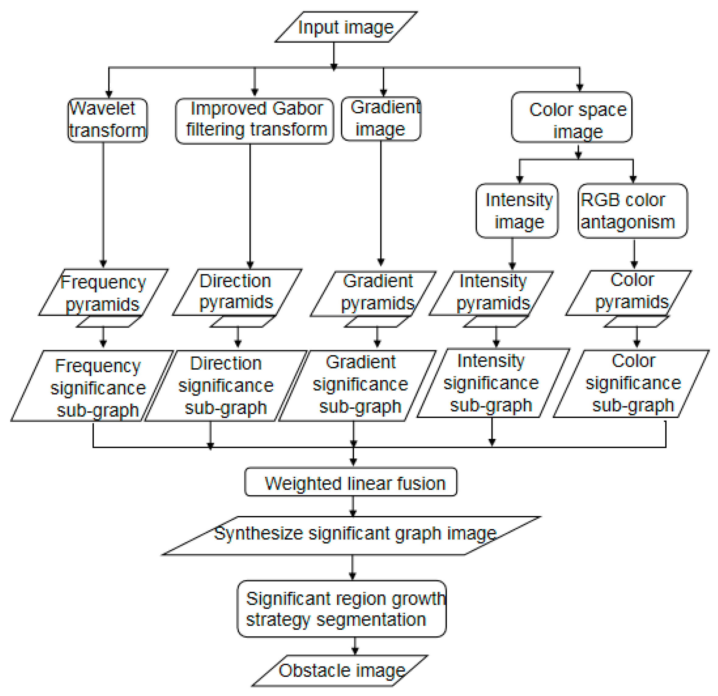
Owing to the different sizes, shapes and colors of the sea surface targets, a single feature cannot be used to obtain a sufficiently descriptive saliency map. Therefore, the attention subgraphs of multi-visual features should be fused. Specifically, a wavelet transform, Gaussian filter and color space transform can be employed to obtain the saliency subgraphs of the high and low frequencies of the target, gradient texture features and luminance and color antagonism features, respectively. The feature subgraphs can be fused using a weighted linear strategy to obtain a comprehensive salient image. Finally, the target region can be segmented through a significant region growth segmentation strategy. The process flow of the specific algorithm is in Figure 2.
3.1. Wavelet Transform to Extract the Frequency Saliency Subgraph
Owing to the difference in the features of sea objects, the Haar wavelet transform is used to decompose the sea surface image to obtain the high and low frequency features and , respectively. In the case of the high-frequency features, the logarithm of the image is considered to obtain the logarithmic spectrum image , which contains the high-frequency information in the image. The logarithmic spectrum is obtained by smoothing the logarithmic spectrum with the mean template and subtracting the logarithmic spectrum from the mean spectrum to obtain the spectral residuals as follows:
where . is the mean value of the filter template, and represents the convolution operation.
According to Equation (9), we can sum the spectral residuals and phase spectra and use the fast Fourier inversion to obtain the wavelet transform related high-frequency characteristic saliency map . Specifically, can be defined as:
3.2. Improved Gabor Filtering to Obtain the Directional Feature Saliency Subgraph
Although the edge information in the directional feature map can be extracted through traditional Gabor filtering, the overall significance of the target is lost. In this work, to realize the directional feature extraction, the exponential function was used instead of the Gabor function. In this case, the exponential function is as follows:
where, denote the pixel coordinates, and . and are the scale factors in the and directions, respectively.
The convolution operation is performed between the sea surface image and exponential function to obtain the feature subgraphs pertaining to different directions . These subgraphs are linearly combined obtain the feature map for the different directions . The significance value of the directional feature graph is calculated using Equations (1) and (2), and the frequency significance subgraph is:
3.3. Gradient Texture Feature Saliency Subgraph
The gradient image reflects the areas in the image that involve notable variations in the edge and texture. Therefore, the gradient significant subgraph is obtained using the gradient texture spectra that was described in Section 3.1 for obtaining the gradient saliency subgraph.
3.4. Color Spatial Feature Saliency Subgraph
The luminance and color antagonism channel feature images for each pixel in the sea surface image are obtained according to the color components of each pixel. Specifically, through the experimental data, we obtain the feature images for luminance , based on the color antagonism channels , and :
where is the color information of a single pixel, and the color feature component of each pixel is , and , respectively.
The saliency subgraphs were obtained by calculating the significant values of the characteristic maps of the luminance, , and color antagonism channels, , and .
3.5. Fusion and Segmentation of the Multi-Visual Feature Salient Graph
Image fusion must be performed to obtain salient images with different features. Herein, we use the normalized linear combination to obtain the multi-visual feature saliency comprehensive graph . The comprehensive graph can be expressed as:
where denotes the weight of each feature, and is the feature salient subgraph. In this experiment, the luminance and color feature subgraphs have larger weights, and the other saliency subgraphs have smaller weights.
Compared to the traditional method, in which adaptive threshold segmentation is performed to obtain binary images and the target area is direct identified based on the binary images, the proposed method is simpler and involves a higher false detection rate. The significant area growth strategy [32] is applied to segment the salient image, to effectively obtain the target image from the salient graph.
4. Experiments
This section describes the experimental validation of the proposed approach. The experimental analysis was performed in two parts. In the first part, we evaluated and analyzed the sea-sky-line detection performance. In the second part, we evaluated and analyzed the performance of the multi-visual feature significance detection for sea-surface objects and compared it with that of the alternative methods. The marine obstacle detection dataset (MOOD) [33] and Singapore maritime dataset (SMD) [34] were selected to realize the simulation testing with an image resolution of . All the experiments were performed on a desktop PC Intel (R)Core(TM)i5-6500 CPU 3.2 GHz processor with MATLAB 2018b on a WIN10 (64-bits) operating system.
4.1. Sea-Sky-Line Detection Performance
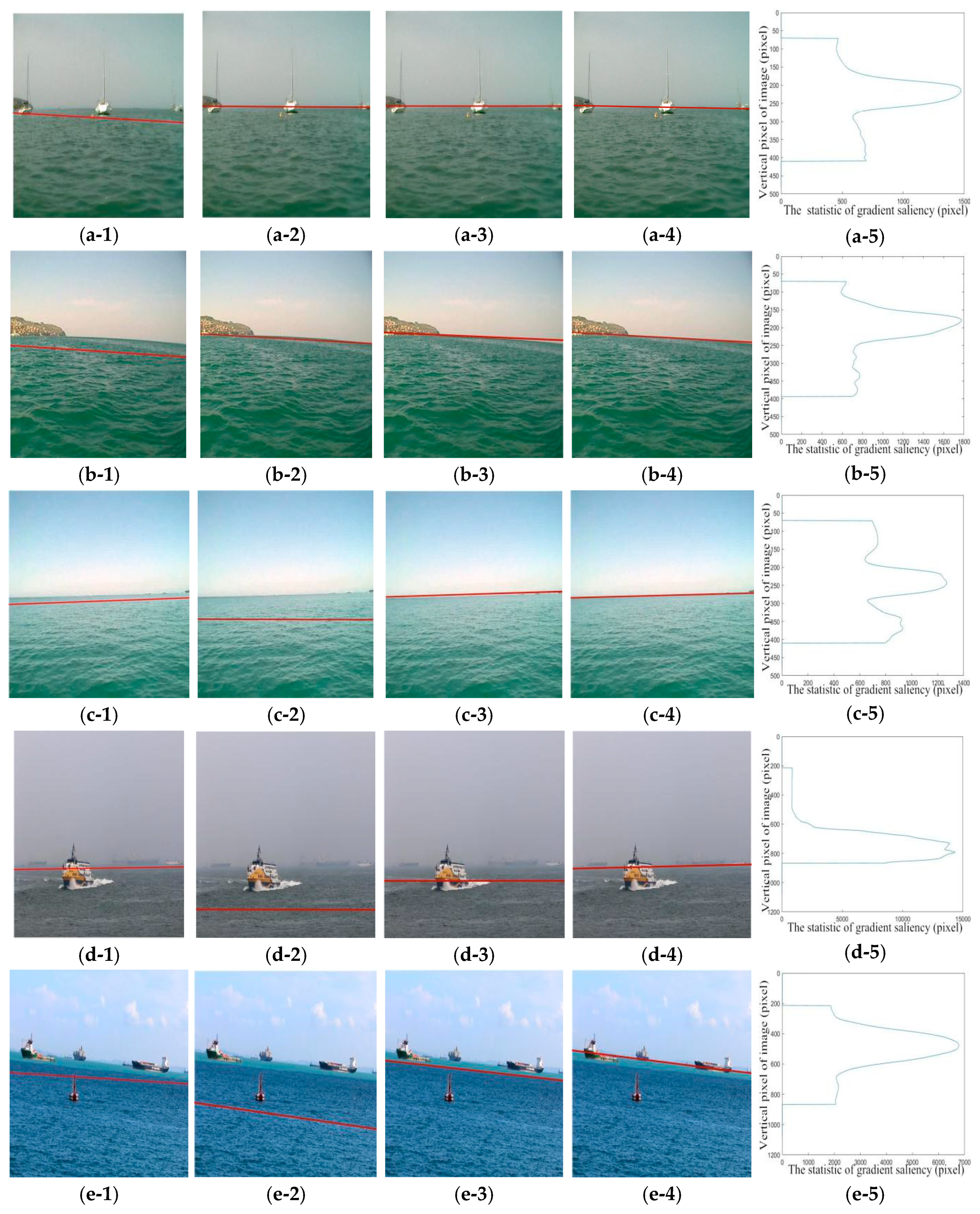
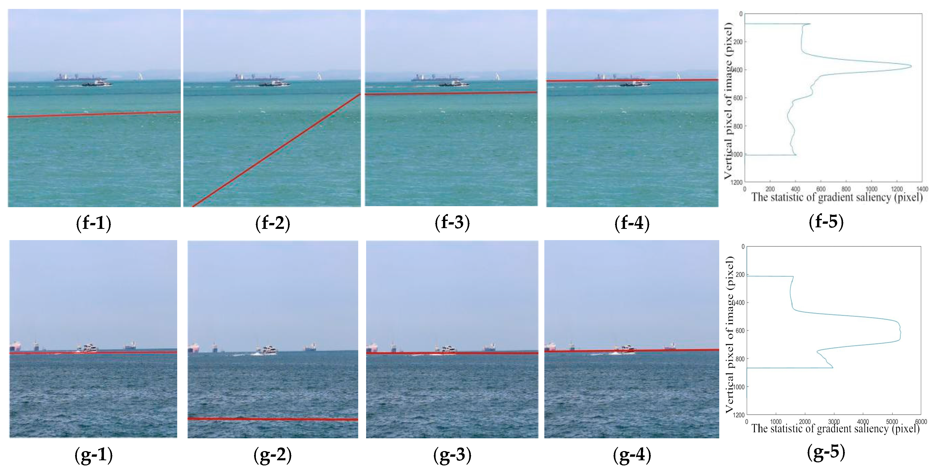
To validate the proposed sea-sky-line detection model, we randomly selected 150 images from the MOOD dataset and video sets from the SMD dataset to compare the sea-sky-line detection performance of the proposed method with that of the Hough algorithm [35], gradient enhancement + Hough algorithm and semantic segmentation based obstacle image-map estimation algorithm (SSM) [36]. The sea-sky-line fitting polynomial was set as 5, and the error threshold of the image pixel was . In general, in the case of the initial sea-sky-line scene images, the influence of factors such as cloud waves, clouds or complex background on the sea-sky-line can be alleviated through filtering by gradient image smoothing. When considerable noise is present in the image, gradient smoothing can help remove the discrete noise. In addition, implementing image pre-processing involving gradient smoothing can strengthen the boundary contrast between the sea and sky regions. The edge saliency of the region surrounding the sea-sky-line is enhanced, and the detection performance is considerably improved. Figure 3 (column 5) shows the gradient significance integral curve of the image. The area corresponding to the peak of the curve corresponds to the row coordinates of the potential region of the sea-sky-line. Furthermore, the proposed method can realize the overall classification of the potential sea-sky-line region and obtain the estimation point of the sea-sky-line. Through the polynomial iterative fitting, the sea-sky-line can be fitted correctly, and the fitted curve can accurately reflect the real position of the sea-sky-line.
Figure 3 (column 2) shows the area of the sea-sky-line obtained using the Hough transform method. In the transformation process, the longest straight-line segment obtained is used to fit the sea-sky-line. Under a low contrast or strong illumination, or the presence of clouds or edge of the obstacles in the sea, the Hough transform can produce numerous straight-line segments, thereby introducing an uncertainty in the sea-sky-line detection. Therefore, the detection results are not satisfactory. The Hough transform combined with the gradient saliency enhancement algorithm can better negate the effect of the background and effectively enhance the edge of the sea-sky-line. The detection results are better than those of the single Hough transform, as shown in Figure 3 (column 3). The SSM algorithm exhibits a high detection speed; however, the Markov chain is considerably dependent on the edge of the previous image, leading to a poor robustness. The sea-sky-line information may be easily lost in the case of jitters, as shown in Figure 3 (column 1). In comparison, the proposed method is more effective and can eliminate the effect of interferences such as cloud waves and sea clutter to correctly detect the position of the sea-sky-line.
Table 1 presents the average detection rate and time in the evaluation of the sea-sky-line detection performance of the four algorithms. The sea-sky-line detection rate of the proposed method is significantly higher than that of the other three algorithms, with the lowest average detection time and highest detection accuracy. These values can satisfy practical application requirements. Therefore, as described in Section 4.2, the proposed method was used to identify the sea-sky-lines and segment the sea surface images. Subsequently, an experiment was performed to compare the visual saliency detection results.
4.2. Visual Detection Performance
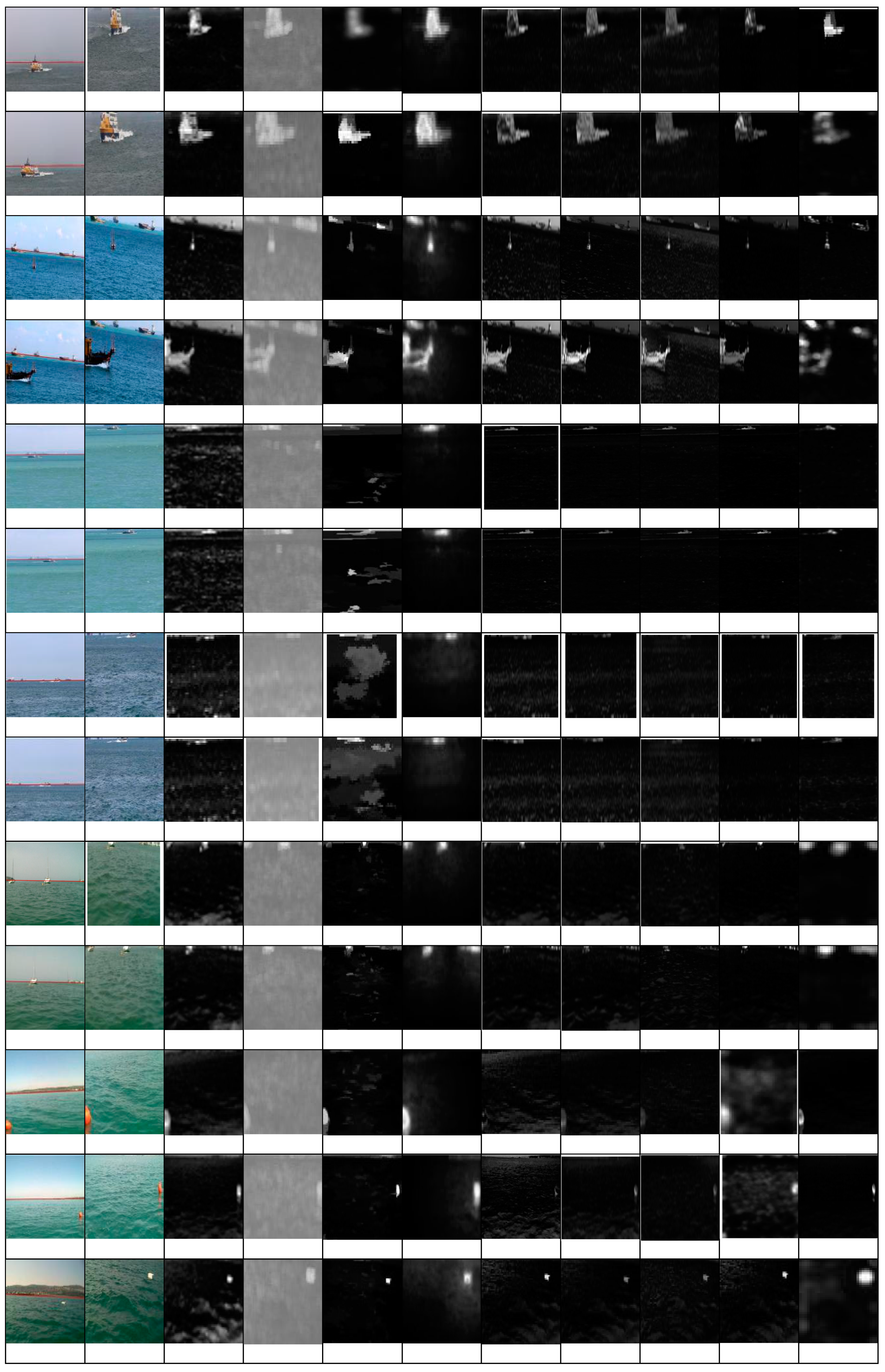
After realizing the sea-sky-line detection segmentation, the proposed method was compared qualitatively and quantitatively with the Random Walk with Restart on Video(RWRV) [28], Attention based on Information Maximization (AIM) [37], Spatiotemporal attention detection(SD) [38], Context-Aware Saliency Detection(CA) [39], Discriminative Regional Feature Integration Approach(DRFI) [40], Spatiotemporal Cues Approach (SC) [41], histogram-based contrast method (HC) [42] and Frequency-tuned Salient Region Detection FT [43] approaches. The parameters of all these models were set according to the publicly available code of the algorithms. Figure 4 shown the saliency maps obtained using the proposed algorithm and other algorithms to enable a qualitative comparison. Column 1 in Figure 4 corresponds to the sea-sky-line images, with the red lines indicating the sea-sky-line. The videos (representative frames shown in Column 1) cover a variety of sea-surface targets. Column 2 shows the sea surface image obtained after sea-sky-line detection segmentation.
The following observations can be made
- (1)
- The saliency detection results for the video frame images with a strong contrast between the target object and background (e.g., rows 1 and 2) are satisfactory. The target information in the saliency feature image is highlighted. Therefore, when a strong contrast exists between the foreground and background, the features of the target can be easily detected.
- (2)
- The performance is relatively weak in the presence of a low contrast or complex background. The RWRV, SC, HC, SD and FT approaches are strongly influenced by the sky background and highlight the sky feature information in the saliency map, as shown in rows 3, 4, 7 and 8. Moreover, the RWRV, AIM, DRFI and FT approaches exhibit a poor robustness against the interference of sea waves. Notable features of sea waves are present in the saliency map, as shown in rows 5, 6 and 13. In the case of small target objects in the sea surface images, the target image may be lost in the saliency maps owing to the influence of the background, as in the case of the SD algorithm in rows 6 and 7.
- (3)
- The proposed algorithm can capture the foreground salient objects more faithfully in the test cases. The target features are prominent in the saliency map. Moreover, the approach is robust against the background interference from the waves and sky. For example, the proposed algorithm achieved a high performance in the case of objects with multiple appearance color information (e.g., rows 1–4), exhibiting relatively high scene complexities. Moreover, the proposed approach can detect small and distinct regions (rows 9, 10, 12, 13).
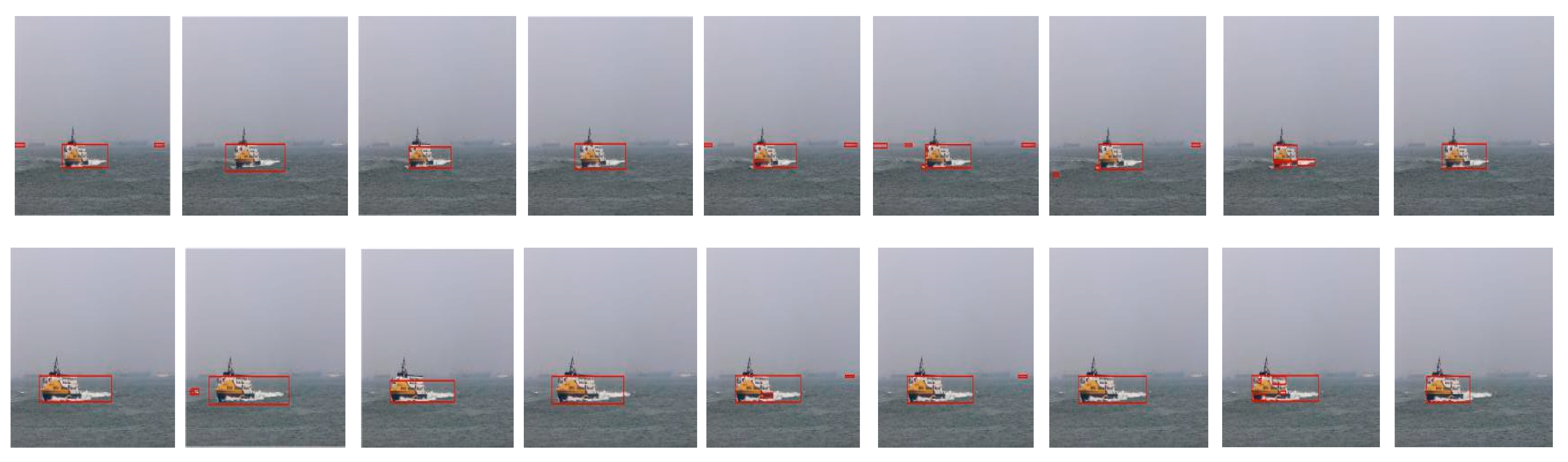
Owing to the use of the saliency region growth strategy for the attention mechanism, the proposed approach can extract the entire saliency target, as shown in Figure 5. The saliency map generated using the proposed method is more visually consistent with the shape, size and location of the ground truth segmentation map than those generated by the other methods. The saliency map tends to highlight the outline of the object regions, and a small amount of the internal information is merged into the foreground.
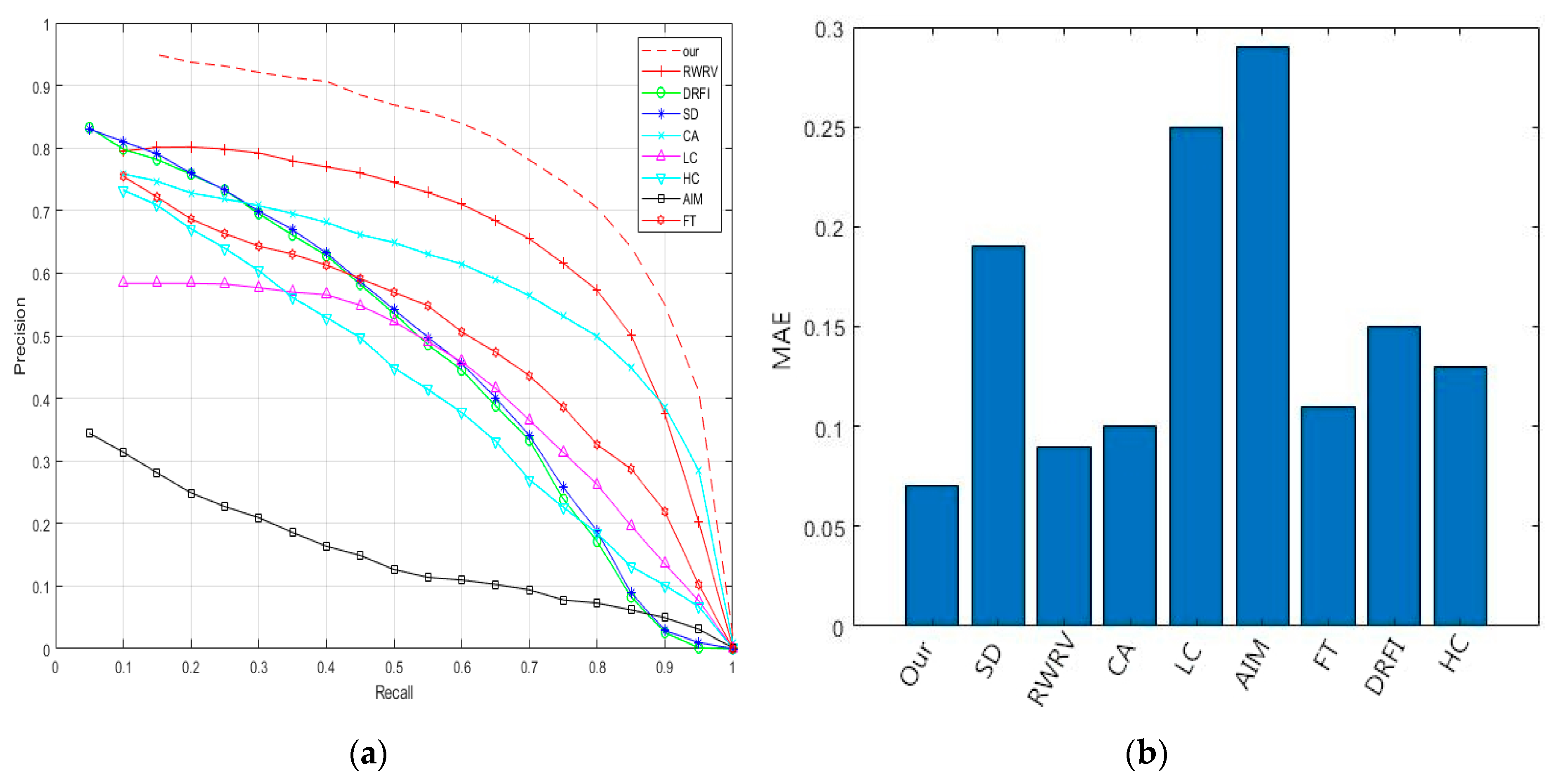
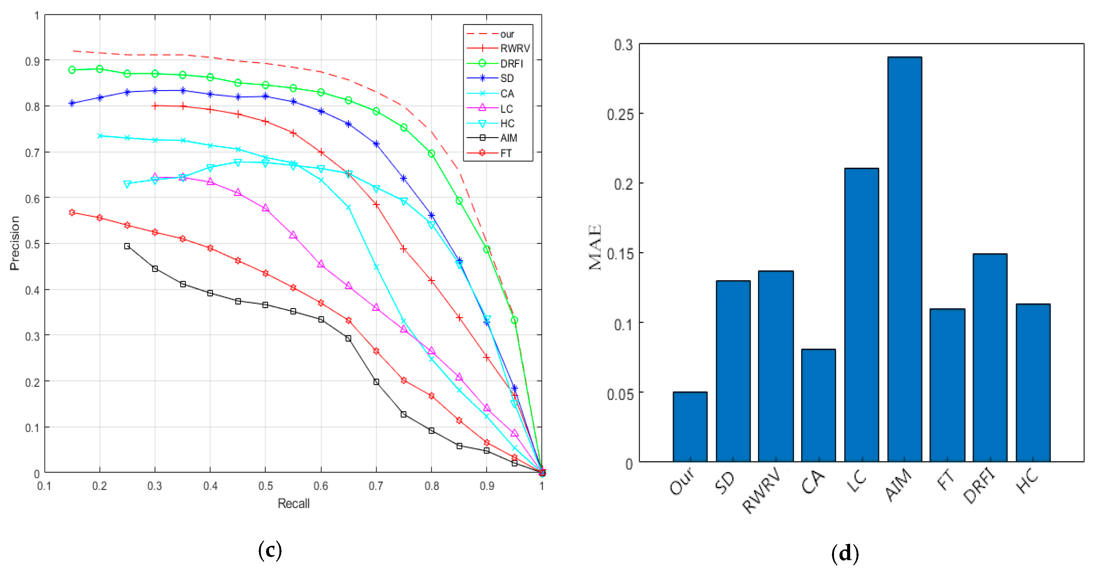
To further evaluate the performance of the proposed method, we evaluated the results based on two widely used criteria, namely, the precision–recall (PR) curve and mean absolute errors (MAEs) [24]. In the precision–recall analysis, the precision is defined as the percentage of the salient pixels correctly assigned, and the recall corresponds to the fraction of the detected salient pixels in relation to the ground truth number of the salient pixels. For each saliency map, the PR curve is obtained using 256 PR pairs, generated by normalizing the threshold from 0 to 1.
The F-measure is a measure of the overall performance, computed using the weighted harmonic of the precision and recall:
where we set to weigh the precision. For each saliency map, we derived a sequence of the F-measure values along the PR curve, with the threshold varying from 0 to 1.
For further comparison, we evaluated the MAE between a continuous saliency map and the binary ground truth for all image/frame pixels, as follows:
where is the number of image/frame pixels. The estimates the approximation degree between the saliency map and ground truth, normalized as [0, 1]. The provides a better estimate of the dissimilarity between the saliency map and ground truth.
The resulting PR curves are shown in Figure 6a,c for the two data sets. The trend of the PR curves for all the methods is consistent. When the threshold is close to 1, the recall values of the AIM, FT, CA and SC are extremely small and decrease to zero. The proposed method exhibits the highest performance, with a precision rate of more than 0.9, which indicates that this method is more precise and responsive to the salient regions. Moreover, the curvature rate of the PR curve of the proposed approach, exhibiting a high recall and high precision, is smaller than that of the curves of the other methods. In addition, the proposed saliency method achieves the highest precision rates, which demonstrates that these saliency maps are more precise and responsive to the actual salient information. The MAE results are presented in Figure 6b,d. The proposed method exhibits the smallest MAE, corresponding to the best performance among all the other approaches. These findings indicate that the proposed method can realize a global optimization for the salient object detection.
5. Conclusions
To address the problems of saliency target detection in maritime images, this paper proposes a saliency detection method based on improved sea-sky-line detection with multi-visual features for sea-surface images. First, the image gradient integration curve is used to estimate the potential sea-sky-line feature points and identify the sea-sky-line in the sea surface image through polynomial iterative fitting. Subsequently, to process the multiple features in sea images, a saliency detection model based on multi-visual features is used to highlight the target and background contrast, to facilitate the saliency detection. Comparative experiments indicated that the proposed algorithm can promptly and accurately segment the sea-sky-line in images. The obtained sea surface image saliency maps can efficiently extract the target saliency of the sea surface image, as indicated by the PR curve and MAEs. The proposed approach can provide guidance for object recognition and localization. Moreover, the proposed framework is highly generalized and can be extended to other maritime image analysis problems.
Future work will be aimed at correlating effective filters with high-level content (e.g., type of movement and object identity). In addition, the effect of white waves (e.g., waves at the stern of the ship, shown in Figure 5) on the saliency detection and segmentation should be eliminated while filtering the wave images to maintain the image details.
Author Contributions
Conceptualization, C.L. and H.Z.; methodology, C.L.; software, C.L.; and Z.Z.; formal analysis, W.C.; investigation, C.L.; resources, C.L. and W.C.; writing—original draft preparation, C.L.; writing—review and editing, C.L. and H.Z. All authors have read and agreed to the published version of the manuscript.
Funding
This research was supported in part by the National Natural Science Foundation of China under Grant 51179074,51679107; the Natural Science Foundation of Fujian provincial under Grant 2018J01495; the Young and Middle-aged Teachers Project of Fujian provincial under Grant JAT170507, JAT170507(p); the Putian Science and Technology bureau project under Grant 2018RP4002; the Xiamen Science and Technology Plan Project under Grant 3502Z20123024.
Acknowledgments
The authors would like to thank Yan Zhang for help.
Conflicts of Interest
The authors declare no conflict of interest.
References
- Bovcon, B.; Mandeljc, R.; Janez, P. Stereo obstacle detection for unmanned surface vehicles by IMU-assisted semantic segmentation. Robot. Auton. Syst. 2018, 104, 1–13. [Google Scholar] [CrossRef] [Green Version]
- Woo, J.; Kim, N. Vision based obstacle detection and collision risk estimation of an unmanned surface vehicle. In Proceedings of the IEEE International Conference on Ubiquitous Robots and Ambient Intelligence, Xi’an, China, 19–22 August 2016; pp. 461–465. [Google Scholar]
- Shin, B.S.; Mou, X.; Mou, W. Vision-based navigation of an unmanned surface vehicle with object detection and tracking abilities. Mach. Vision Appl. 2017, 29, 95–112. [Google Scholar] [CrossRef]
- Kong, X.; Liu, L.; Qian, Y. Automatic detection of sea-sky horizon line and small targets in maritime infrared imagery. Infrared Phys. Technol. 2016, 76, 185–199. [Google Scholar] [CrossRef]
- Wang, B.; Su, Y.; Wan, L. A sea-sky line detection method for unmanned surface vehicles based on gradient saliency. Sensors 2016, 16, 543. [Google Scholar] [CrossRef] [Green Version]
- Ma, T.; Ma, J. A sea-sky line detection method based on line segment detector and Hough transform. In Proceedings of the IEEE International Conference on Computer and Communications, Helsinki, Finland, 21–23 August 2017; pp. 700–703. [Google Scholar]
- Kim, S.; Lee, J. Small infrared target detection by region adaptive clutter rejection for sea-based infrared search and track. Sensors 2014, 14, 13210–13242. [Google Scholar] [CrossRef] [PubMed]
- Tang, D.; Sun, G.; Wang, D.H.; Niu, Z.D.; Chen, Z.P. Research on infrared ship detection method in sea-sky background. In Proceedings of the International Symposium on Photoelectronic Detection and Imaging 2013: Infrared Imaging and Applications, Beijing, China, 25–28 June 2013; pp. 89072H-1–89072H-10. [Google Scholar]
- Shen, Y.; Krusienski, D.J.; Li, J.; Rahman, Z. A Hierarchical Horizon Detection Algorithm. IEEE Geosci. Remote Sens. Lett. 2013, 10, 111–114. [Google Scholar] [CrossRef]
- Dai, Y.S.; Liu, B.; Li, L.G.; Jin, J.C.; Sun, W.F.; Shao, F. Sea-sky-line detection based on local Otsu segmentation and Hough transform. Opto Electron. Eng. 2018, 45, 180039. [Google Scholar]
- Jiang, C.L.; Jiang, H.H.; Zhang, C.L.; Wang, J. A new method of sea-sky-line detection. In Proceedings of the Third IEEE International Symposium on Intelligent Information Technology and Security Informatics, NanChang, China, 21–22 November 2010; pp. 740–743. [Google Scholar]
- Jiao, J.; Lu, H.; Wang, Z. L0 Gradient Smoothing and Bimodal Histogram Analysis: A Robust Method for Sea-sky-line Detectio. In Proceedings of the ACM Multimedia Asia, Beijing China, 16–18 December 2019; pp. 1–6. [Google Scholar]
- Jeong, C.Y.; Yang, H.S.; Moon, K. A novel approach for detecting the horizon using a convolutional neural network and multi-scale edge detection. Multidimens. Syst. Signal Process. 2019, 30, 1187–1204. [Google Scholar] [CrossRef]
- Zou, X.; Xiao, C.; Zhan, W.; Zhou, C.; Xiu, S.; Yuan, H. A Novel Water-Shore-Line Detection Method for USV Autonomous Navigation. Sensors 2020, 20, 1682. [Google Scholar] [CrossRef] [Green Version]
- Gilbert, C.D.; Li, W. Top-down influences on visual processing. Nat. Rev. Neurosci. 2013, 14, 350–363. [Google Scholar] [CrossRef]
- Navalpakkam, V.; Itti, L. Top–down attention selection is fine grained. J. Vis. 2006, 6, 1180–1193. [Google Scholar] [CrossRef] [PubMed] [Green Version]
- Yan, Q.; Xu, L.; Shi, J. Hierarchical saliency detection. In Proceedings of the IEEE Computer Vision and Pattern Recognition, Portland, OR, USA, 23–28 June 2013; pp. 1155–1162. [Google Scholar]
- Hou, X.; Zhang, L. Saliency detection: A spectral residual approach. In Proceedings of the IEEE Computer Vision and Pattern Recognition, Minneapolis, MN, USA, 17–22 June 2007; pp. 1–8. [Google Scholar]
- Schauerte, B.; Stiefelhagen, R. Quaternion-Based spectral saliency detection for eye fixation prediction. In Proceedings of the European Conference on Computer Vision, Florence, Italy, 12–13 November 2012; pp. 116–129. [Google Scholar]
- Itti, L.; Koch, C.; Niebur, E. A model of saliency-based visual attention for rapid scene analysis. IEEE Trans. Pattern Anal. Mach. Intell. 1998, 20, 1254–1259. [Google Scholar] [CrossRef] [Green Version]
- Rinki, A.; Agrawal, R.K.; Navjot, S. A novel approach for salient object detection using double-density dual-tree complex wavelet transform in conjunction with superpixel segmentation. Knowl. Inf. Syst. 2018, 60, 327–361. [Google Scholar]
- Chen, Y.; Zou, W.; Tang, Y.; Li, X.; Xu, C.; Komodakis, N. SCOM: Spatiotemporal Constrained Optimization for Salient Object Detection. IEEE Trans. Image Process. 2018, 27, 3345–3357. [Google Scholar] [CrossRef]
- Zhang, W.; Yao, Z.F.; Gao, Y.K. A deep convolutional network for saliency object detection with balanced accuracy and high efficiency. J. Electr. Syst. Inf. Technol. 2020, 42, 1201–1208. [Google Scholar]
- Wang, W.; Shen, J.; Shao, L. Video Salient Object Detection via Fully Convolutional Networks. IEEE Trans. Image Process. 2017, 27, 38–49. [Google Scholar] [CrossRef] [PubMed] [Green Version]
- Singh, M.; Govil, M.C.; Pilli, E.S. SOD-CED: Salient Object Detection for Noisy Images using Convolution Encoder Decoder. IET Comput. Vis. 2019, 13, 578–587. [Google Scholar] [CrossRef]
- Cheng, M.; Zhang, G.; Mitra, N.J.; Huang, X.; Hu, S. Global contrast based salient region detection. IEEE Trans. Pattern Anal. Mach. Intell. 2014, 37, 569–582. [Google Scholar] [CrossRef] [Green Version]
- Li, J.; Gao, W. Visual Saliency Computation A Machine Learning Perspective; Springer Publishing Company, Inc.: New York, NY, USA, 2014. [Google Scholar]
- Kim, H.; Kim, Y.; Sim, J.Y. Spatiotemporal Saliency Detection for Video Sequences Based on Random Walk With Restart. IEEE Trans. Image Process. 2015, 24, 2552–2564. [Google Scholar] [CrossRef] [PubMed]
- Singh, N.; Mishra, K.K.; Bhatia, S. SEAM—An improved environmental adaptation method with real parameter coding for salient object detection. Multimed. Tools Appl. 2020, 79, 12995–13010. [Google Scholar] [CrossRef]
- Gonzalez, R.C.; Woods, R.E. Digital Image Processing, 3rd ed.; Prentice-Hall, Inc.: Upper Saddle River, NJ, USA, 2007. [Google Scholar]
- Zou, R.B.; Shi, C.C. A Sea-Sky Line Identification Algorithem Based on Shearlets for Infrared Image. Adv. Mate. Res. 2013, 846–847, 1031–1035. [Google Scholar] [CrossRef]
- Lin, C.; He, B.W.; Dong, S. An in door object fast detection method based on visual attention mechanism of fusion depth information in RGB image. Chin. J. Lasers 2014, 41, 205–210. [Google Scholar]
- Available online: http://www.vicos.si/Downloads/MODD (accessed on 31 March 2015).
- Prasad, D.K.; Rajan, D.; Rachmawati, L.; Rajabally, E.; Quek, C. Video Processing From Electro-Optical Sensors for Object Detection and Tracking in a Maritime Environment: A Survey. IEEE Trans. Intell. Transp. Syst. 2017, 18, 1993–2016. [Google Scholar] [CrossRef] [Green Version]
- Bowe, A.N. Study of sea-sky-line detection algorithm based on Hough transform. Infrared Technol. 2015, 37, 196–199. [Google Scholar]
- Kristan, M.; Kenk, V.S.; Kovacic, S.; Pers, J. Fast Image-Based Obstacle Detection from Unmanned Surface Vehicles. IEEE Trans. Cybern. 2016, 46, 641–654. [Google Scholar] [CrossRef] [PubMed] [Green Version]
- Bruce, N.D. Saliency, attention and visual search: An information theoretic approach. J. Vis. 2009, 9, 51. [Google Scholar] [CrossRef] [PubMed]
- Achanta, R.; Estrada, F.; Wils, P. Salient Region Detection and Segmentation. In Proceedings of the 6th International Conference on Computer Vision Systems, Santorini, Greece, 12–15 May 2008; pp. 66–75. [Google Scholar]
- Goferman, S.; Zelnikmanor, L.; Tal, A. Context-Aware Saliency Detection. IEEE Trans. Pattern Anal. Mach. Intell. 2012, 34, 1915–1926. [Google Scholar] [CrossRef] [Green Version]
- Wang, J.D.; Jiang, H.Z.; Yuan, Z.J. Salient Object Detection: A Discriminative Regional Feature Integration Approach. In Proceedings of the IEEE Conference on Computer Vision and Pattern Recognition (CVPR), Honolulu, HI, USA, 21–26 July 2017; Volume 1, pp. 2083–2090. [Google Scholar]
- Zhai, Y.; Shah, M. Visual attention detection in video sequences using spatiotemporal cues. In Proceedings of the 14th Annual ACM International Conference on Multimedia, Santa Barbara, CA, USA, 23–27 October 2006; pp. 815–824. [Google Scholar]
- Cheng, M.M.; Zhang, G.X.; Mitra, N.J. Global contrast based salient region detection. In Proceedings of the Computer Vision and Pattern Recognition, Providence, RI, USA, 20–25 June 2011; pp. 409–416. [Google Scholar]
- Achanta, R.; Hemami, S.S.; Estrada, F.J.; Susstrunk, S. Frequency-tuned salient region detection. In Proceedings of the Computer Vision and Pattern Recognition, Miami, FL, USA, 20–25 June 2009; pp. 1597–1604. [Google Scholar]
Figure 1.
Semantic regions in an image. The bottom ① and top ③ regions represent water and the sky, respectively. The middle ② component can represent land, parked boats, a haze above the horizon or a mixture of these.
Figure 1.
Semantic regions in an image. The bottom ① and top ③ regions represent water and the sky, respectively. The middle ② component can represent land, parked boats, a haze above the horizon or a mixture of these.

Figure 2.
Process flow of the saliency detection model for multi-visual feature fusion.

Figure 3.
Detection results of different sea-sky-line detection methods for datasets. (Column 1) Show the images processed using the SSM. (Column 2) Show the images processed using the Hough transformation algorithm. (Column 3) Show the images processed using gradient saliency enhancement and Hough algorithm. (Column 4) Show the images processed using our algorithm. (Column 5) Show the images processed using integral curve of gradient saliency.


Figure 4.
Examples of saliency maps generated using eight state-of-the-art models and the proposed model. Columns 1–8 and 9–13 correspond to the SMD and MOOD datasets. Columns 1–11 correspond to the sea-sky-line images, segmentation images and the images processed using the RWRV, AIM, DRFI, CA, SC, HC, SD, FT and proposed algorithms, respectively.

Figure 5.
Sea surface image saliency target segmentation results for different algorithms. Columns 1–9 shows the images processed using the RWRV, AIM, DRFI, CA, SC, HC, SD, FT and proposed algorithms, respectively.
Figure 5.
Sea surface image saliency target segmentation results for different algorithms. Columns 1–9 shows the images processed using the RWRV, AIM, DRFI, CA, SC, HC, SD, FT and proposed algorithms, respectively.

Figure 6.
Precision–recall (PR) curves and mean absolute errors (MAEs) for the two datasets generated using different configurations. (a) PR curve and (b) MAE for MOOD. (c) PR curve and (d) MAE for SMD.
Figure 6.
Precision–recall (PR) curves and mean absolute errors (MAEs) for the two datasets generated using different configurations. (a) PR curve and (b) MAE for MOOD. (c) PR curve and (d) MAE for SMD.


Table 1.
Comparison of the detection performance of different methods.
| Method | SSM | Hough Transformation | Gradient Saliency Enhancement + Hough | Proposed |
|---|---|---|---|---|
| Average detection/% | 48.6 | 52.6 | 76.8 | 96.3 |
| Average detection time/s | 1.18 | 2.59 | 2.62 | 1.05 |
Publisher’s Note: MDPI stays neutral with regard to jurisdictional claims in published maps and institutional affiliations. |
© 2020 by the authors. Licensee MDPI, Basel, Switzerland. This article is an open access article distributed under the terms and conditions of the Creative Commons Attribution (CC BY) license (http://creativecommons.org/licenses/by/4.0/).
Share and Cite
MDPI and ACS Style
Lin, C.; Chen, W.; Zhou, H. Multi-Visual Feature Saliency Detection for Sea-Surface Targets through Improved Sea-Sky-Line Detection. J. Mar. Sci. Eng. 2020, 8, 799. https://doi.org/10.3390/jmse8100799
AMA Style
Lin C, Chen W, Zhou H. Multi-Visual Feature Saliency Detection for Sea-Surface Targets through Improved Sea-Sky-Line Detection. Journal of Marine Science and Engineering. 2020; 8(10):799. https://doi.org/10.3390/jmse8100799
Chicago/Turabian StyleLin, Chang, Wu Chen, and Haifeng Zhou. 2020. "Multi-Visual Feature Saliency Detection for Sea-Surface Targets through Improved Sea-Sky-Line Detection" Journal of Marine Science and Engineering 8, no. 10: 799. https://doi.org/10.3390/jmse8100799
Note that from the first issue of 2016, this journal uses article numbers instead of page numbers. See further details here.