LoS Theoretical and Experimental MIMO Study from 1–40 GHz in Indoor Environments

Abstract

In this work, line-of-sight multiple-input multiple-output (MIMO) measurements in the frequency range from 1 GHz to 40 GHz are presented for an indoor environment in the scope of new 5G bands. For the sake of comparison, the measured radio channels are reproduced with great accuracy using ray-tracing techniques by tuning all propagation mechanisms. The relative received power, root mean square of the delay spread (RMS DS) and K-factor provide an insight of how propagation behaves in indoor scenarios within a large and contiguous frequency band. Results show that a decay factor behaves nearly constant with frequency and the RMS DS is quite sensible to frequency. From these results, faithful one-slope 5G models are proposed. Finally, the contribution of the simulated propagation mechanisms to the radio channel is investigated which suggests that the simulation of the low-mmW radio channel can be simplified.

1. Introduction

Millimeter wave (mm-wave) frequencies for 5G and beyond has gained considerable attention within the wireless industry. The main reason is the availability of large bandwidths from 30 GHz to 300 GHz that will be used to increase the wireless binary rates above 10 Gbps [1]. The large blocks of spectrum in the mm-wave range allows the designers to tradeoff spectral efficiency for bandwidth in the early stages of deployment of this technology. Furthermore, the traditional sub-6 GHz bands cannot accommodate the enormous amount of data to be generated in 5G respect to previous generations.

The mobile data will reasonably grow up from 12 exabytes per month at the end of 2017 up to 77 exabytes per month in 2022 [2]. The International Telecommunication Union (ITU) forecasted in its report of 2015 a global mobile data traffic of 5 zettabytes by the end of the 2020s [3]. Thus, there is no doubt that a more comprehensive understanding of radio wave propagation is crucial to any further development of wireless networks. It is important to highlight the importance of advanced techniques as massive line-of-sight MIMO to achieve higher bit rates as seen in [4] in vehicular communications, [5,6,7] in wireless sensor networks and [8] in ultra-dense networks; without a thorough analysis of the radio channel, massive MIMO will be of difficult application [9].

The World Radio Conference established 5G frequency bands in WRC’15 [10], and more recently in WRC’19 [11]. Moreover, the first phase of EU’s Horizon 2020 5G Public Private Partnership initiative is investigating the 6–100 GHz frequencies, including mm-wave frequencies, for 5G’s ultra-high data rate mobile broadband, among other applications. While significant studies of the channel characteristics are available in the 28 GHz, 38 GHz, and 60 GHz bands for indoor and outdoor environments [12,13,14,15,16,17], only a few trials have been conducted in other mm-wave bands and for outdoor and outdoor–indoor environments, as well as scenarios with mobility. However, due to the higher frequencies and wider bandwidths, compared to existing standards below 6 GHz as 4G Long Term Evolution (LTE) and Wireless Local Area Network (WLAN), mm-wave applications need specific considerations.

Usually, the experimental analysis of the channel is completed using simulation tools. Ray-tracing and ray-launching techniques are among the most useful ones, due to their good tradeoff between accuracy and computational effort. Another advantage lies in the completeness of the analysis; path loss (PL), angular and delay parameters, frequency parameters as well as statistical parameters can be extracted from ray based simulations. Regarding the simulation of the mm-wave channel using the mentioned techniques, different analysis were done at 2 GHz and 18 GHz [18], 28 GHz [19], 28 GHz and 38 GHz [20] and 60 GHz [21].

To the best of the authors’ knowledge, little research dealing with MIMO propagation and channel modeling in the whole 1–40 GHz has been reported [22]. As a preliminary work from the authors in [23], the whole band was measured and several channel parameters were analyzed; particularly, the PL, the 1-slope model of the PL, the RMS DS, the 1-slope model of the RMS DS, and the K-factor were extracted. To compare the behavior of the channel throughout the whole band, the measured band was divided in sub-bands centered at 2 GHz, 10 GHz, 20 GHz, 30 GHz, 40 GHz with a 2 GHz bandwidth in all cases.

Some works have analyzed the channel behavior in specific bands between 1 GHz and 40 GHz; for example, the path loss was studied at 26 GHz and 39 GHz in [24] and at 28 GHz in [25,26,27,28], but a comparison between the path loss model values of different sub-bands is still missing in the literature; we can find the same absence in the RMS DS studies; analysis of delay dispersion at specific frequencies or sub-bands can be found as, for instance, the work carried out in [25] and [28] at 28 GHz and in [29] at 26 GHz. Therefore, the objectives of the paper are the following. First, this paper presents a 1–40 GHz analysis in a series of sub-bands covering the complete band. Secondly, a specific analysis in the main WRC’15/19 bands is presented. The core microwave bands were selected in WRC’15 to fulfill the increase in traffic requirements for usual dense urban networks. The 24.25–27.5 GHz and 37–43.5 GHz bands were identified by the WRC’19. These two low-mmW bands provide an additional 3.25 GHz and 6.5 GHz of contiguous blocks of spectrum to enable the 5G enhanced mobile broadband (eMBB) experience. Thus, the selected bands are the microwave band between 3.3–4.99 GHz, which includes the C-band and the 4.8–4.99 GHz band, and the low-mmW 24.25–27.5 GHz and 37–43.5 GHz bands. Moreover, following our previous work [23], we show models of the RMS DS versus the transmitter-receiver distance in logarithmic units which can be useful to predict the time dispersion in indoor environments. To fulfill the first two objectives a frequency based wideband measurement system was used; a calibration step was performed to guarantee the precision in all measured positions and the antenna patterns were carefully measured to extract their effect from the channel parameters. Finally, the third principal aim of the work is to show, thanks to an accurate ray-tracing tool, what are the main propagation mechanisms contributing to the radio channel. A tunning phase was applied to find the best diffuse scattering model values and appropriate permittivity values were assigned to the materials present in the scenario to achieve the desired accuracy.

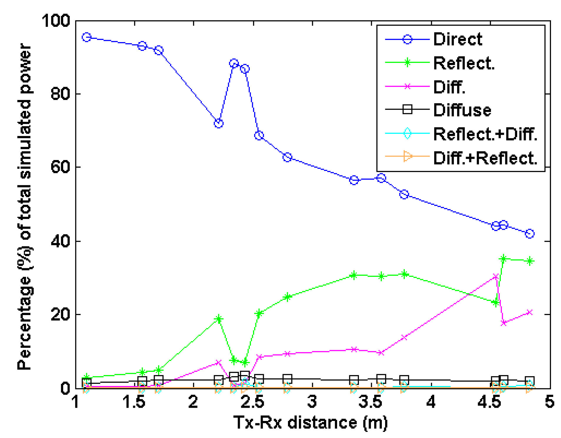
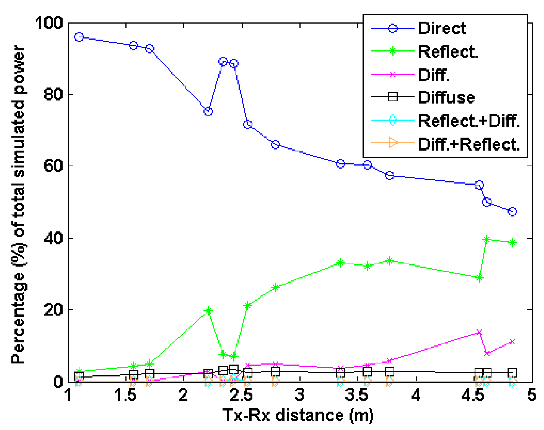
The paper is organized as follows. Section 2 describes the experimental setting. Section 3 presents PL and K-factor. Section 4 shows the RMS DS analysis. Section 5 shows the comparison with ray tracing simulations; the simulation results for WRC bands are included in Appendix A. Finally, in Section 6 the conclusions are explained.

Notations: all magnitudes are written in italics. The symbol $\overline{}$ denotes average, the symbol $\langle \rangle$ represents the expectation operator and the symbol $| |$ denotes absolute value. The base-10 logarithm is represented as log10. The PL and relative received power are expressed in dB, the frequency in GHz, the K factor in dB and the delay spread parameters in nanoseconds.

2. Description of the Experimental Setup

2.1. Scenario

The scenario for the measurements is a laboratory of the Universidad Politécnica de Cartagena (UPCT) as shown in Figure 1. The dimensions of the lab are 9.1 × 4.8 × 4.1 m, and cupboards, desks, chairs, and shelves can be found as furniture. The walls are made of plasterboard, and the floor and ceiling are made of concrete.

Figure 2 depicts a map of the scenario with all measured positions. For the measurements, one position is assumed as an access point and several user positions are uniformly distributed around the room and marked as 1 to 14. In all the experiments, a line of sight (LoS) exists.

In

Table 1. Distance to the walls (A, C) and to either the cupboard or the door (B) of each measured position. The uniform rectangular array (URA) is the receiver. The uniform linear array (ULA) is the transmitter.

Tx Position	A (m)	B (m)	C (m)
1	3.437	1.621	1.295
2	2.264	2.041	2.571
3	1.478	2.040	3.368
4	1.449	3.226	3.380
5	2.264	3.214	2.582
6	3.071	2.891	1.780
7	3.074	4.071	1.767
8	2.276	4.421	2.564
9	1.462	4.452	3.371
10	1.469	5.703	3.359
11	2.269	5.639	2.562
12	3.085	5.283	1.748
13	1.457	6.840	3.364
14	2.259	6.856	2.566
URA	3.630	6.047	1.191
Heights (from top of the antenna)
URA	1.44 m	-	-
ULA	1.33 m	-	-

the distance to the walls of each one of the assumed user positions and the location data of the considered access point are shown.

2.2. Equipment—1–40 GHz

All measurements have been performed using a commercial vector network analyzer (VNA) (Rohde and Schwarz ZVA 10 MHz–67 GHz). To reach all locations in the room an additional radio over fiber (RoF) link (EMCORE, Optiva OTS-2, 40 GHz [30]) has been used. The number of frequency points is 8192, and the intermediate frequency is 100 Hz. Ultra-wideband Omnidirectional Antennas (STEATITE Q-PAR ANTENNAS, 0.8–40 GHz, [31]) have been used at the transmitter (Tx) and receiver (Rx), with vertical polarization and omnidirectional radiation pattern in the horizontal plane. The antenna patterns were measured in an anechoic chamber at 17 different frequencies between 1 GHz and 40 GHz. The antenna gains range from −2.2 dBi to 6.9 dBi and the 3 dB beam width from 20 to 140 degrees. In Figure 3, the measured antenna pattern in dB is shown for four different frequencies. All remain details of the measurement setup can be found in [23,32].

Table 2. Configuration of the channel sounder.

Frequency (GHz)	Bandwidth (GHz)	IF (Hz)	Number of Points
1–40	39	100	8192

summarizes all the configuration of the channel sounder parameters. All measurements are available online in the link included in the Supplementary Materials Section.

2.3. System Configuration

In each position, the Tx and Rx antennas are moved virtually using a uniform rectangular array (URA) and a uniform linear array (ULA), respectively. For the ULA, ten elements were equally spaced along the Y direction; for the URA, measurements were performed over a 6 × 6 uniform rectangular grid along the X and Y directions. The inter-element distance was set to 3 mm for both arrays which is less than λ/2 at 40 GHz. The Y direction corresponds to the vertical axis of Figure 2.

3. Path Loss and K-Factor

The power delay profile (PDP), represented as $P(\tau )$ is computed by averaging, spatially or temporally, the channel impulse response, $h\left(t,\tau \right)$ over a local area:

$$P(\tau )=\overline{{\left|h\left(t,\tau \right)\right|}^2},$$

(1)

where t is the time variable and τ is the delay.

The channel impulse response $h\left(t,\tau \right)$ is obtained by applying the inverse Fourier transform to the frequency response $H\left(f\right)$. In this work, the PDP used to compute the delay parameters is obtained by applying the Hanning window in the frequency domain. This method improves the identification of the multipath components. The path loss is computed without applying the Hanning window so the energy is not altered. 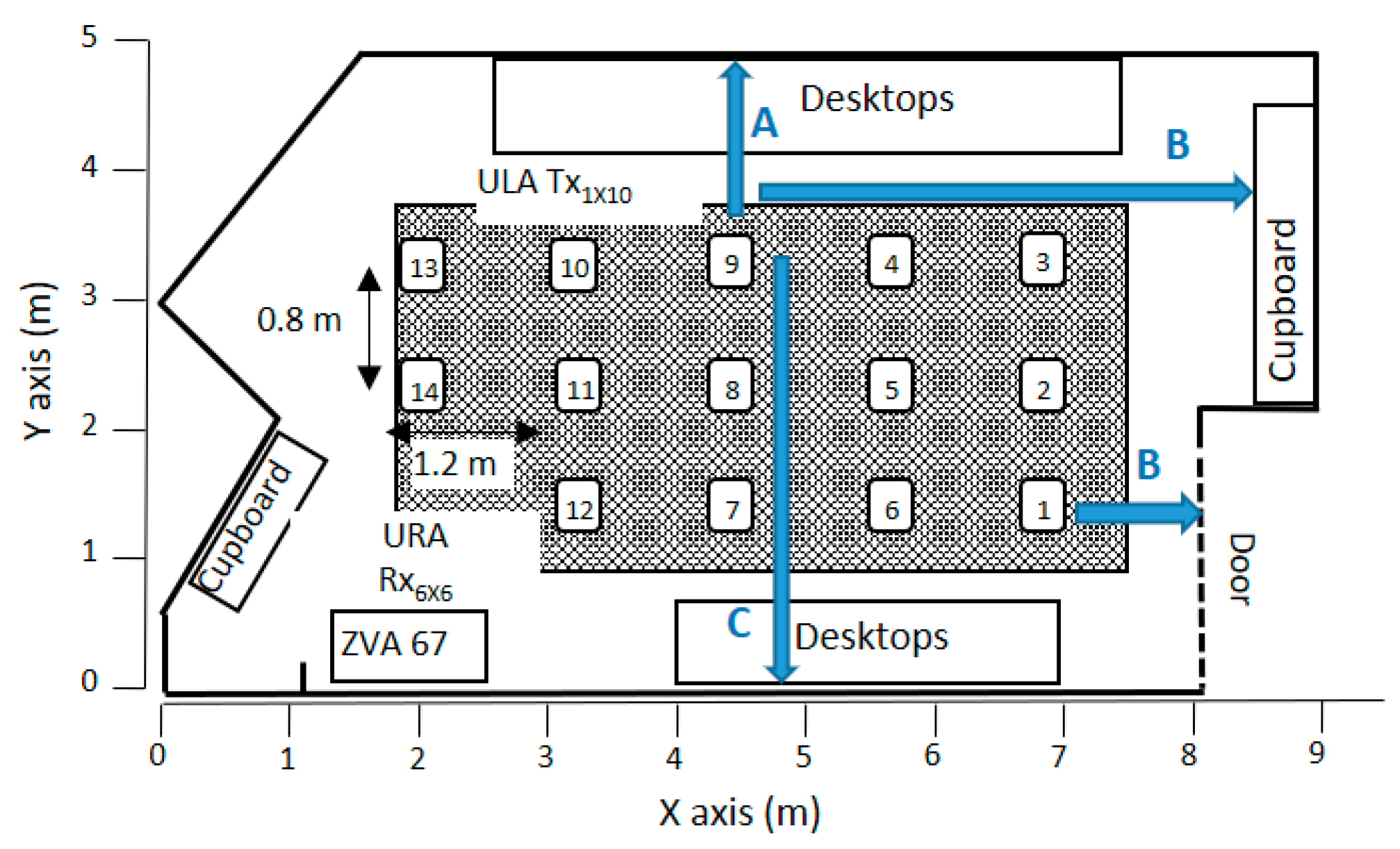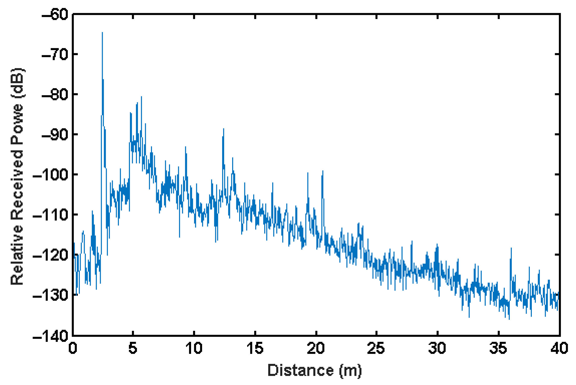Figure 4 depicts the PDP for a given position (number 10 in Figure 2) using all measured bandwidth (see Table 2). In the horizontal axis, the distance in meters is shown by multiplying the delay τ by the speed c. Due to the large bandwidth used, all main multipath components are clearly differentiated.

From the power delay profile in time domain, or from the transfer function in frequency domain, the wideband PL can be computed either by integrating in delay domain or averaging in frequency, respectively. The measurements include the antenna effect; therefore, the antenna influence should be extracted from the measurements. The antenna gain depends on the frequency and the direction whereas the PL includes the effect in all frequencies of the bandwidth of all multipath components coming from different directions. Therefore, an estimation of the antenna effect has to be used; we computed this effect as the mean of the antenna gain in all frequencies and the mean in the azimuthal plane, the plane where the main multipath components and the direct ray are present. Thus, two values G_tx and G_rx, are found for the transmitter and receiver. The path loss equation is:

$$PL=-\langle |H\left(f\right){|}^2{\rangle }_f+G_{rx}+G_{tx}=-\langle |p\left(\tau \right){|}^2{\rangle }_{\tau }+G_{rx}+G_{tx},$$

(2)

where $\langle \rangle$ the expectation (average) operator, f is the frequency, and τ is the delay.

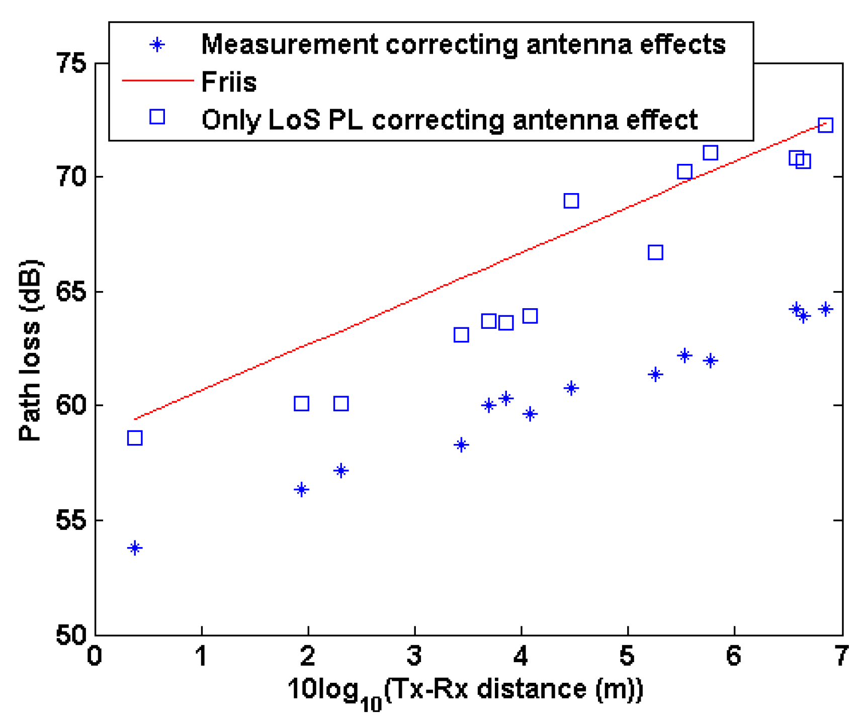
The PL of one specific component in the time domain can be extracted by applying the time gating technique. It is interesting to compare the total wideband PL with the LoS component PL as seen in Figure 5. For the sake of comparison, we have included in Figure 5 the PL evaluated using the Friis model which is observed to be in rather good agreement with the estimated LoS PL. Furthermore, due to the large bandwidth more energy is received from specular components, leading to a low K-factor as it will be shown later.

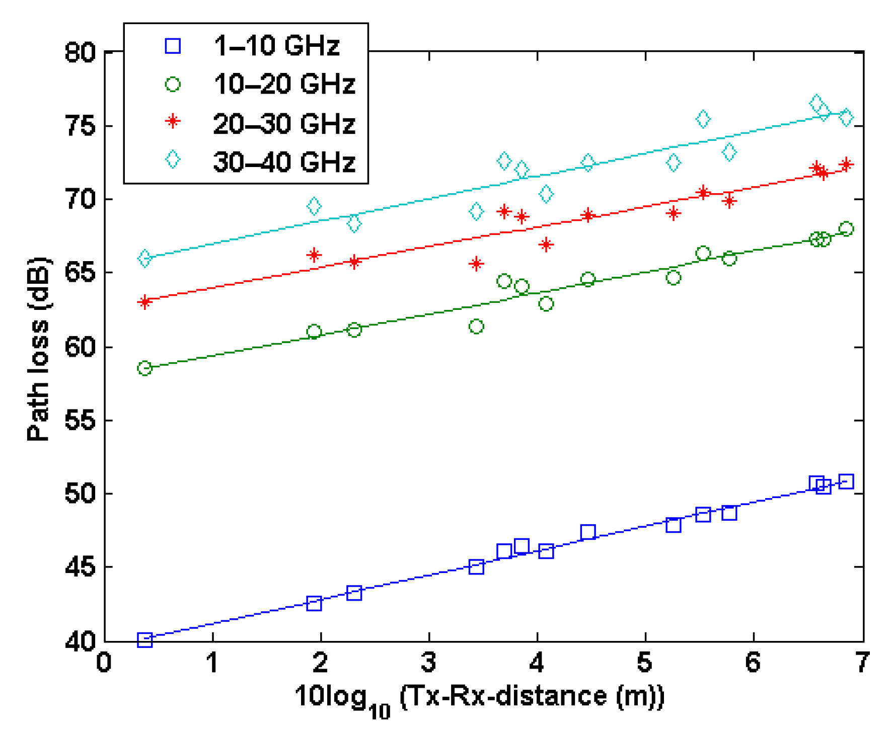
In order to study different bands, we have focused on central frequencies 5 GHz, 15 GHz, 25 GHz and 35 GHz with a 10 GHz bandwidth. The following expression has been used for computing the 1-slope model (Floating-Intercept (FI) path loss).

$$L=L_0+10n\times {\log }_{10}\left(d\right){ + \mathrm{X}}_{\sigma } \left(\mathrm{dB}\right),$$

(3)

where:

• L₀ (in dB) and n are adjustment parameters;
• d (in meters) is the distance between Tx and Rx, and
• X_σ (in dB), a Gaussian random variable with zero means and standard deviation σ (in dB).

Figure 6 shows the relative received power mentioned bands and their corresponding 1-slope models.

The slope parameters of the model can be seen in

Table 3. 1-slope model of the pass lose (PL) for several bands extracted from the 1–40 GHz measured band. The standard deviation and R² parameters are also shown.

Band	n	L0 (dB)	σX (dB)	R2
1–10 GHz	1.66	39.50	0.32	0.99
10–20 GHz	1.42	57.92	0.68	0.94
20–30 GHz	1.25	62.65	0.86	0.90
30–40 GHz	1.54	65.42	1.05	0.88

. The coefficient of determination R² indicates how linear the relation between variables is. We observe a nearly constant decay factor (n), lower than 2 in almost all cases. This low value corresponds to typical indoor values in small distances, similar to those measured in [22,24,25,26,27,28,33], as seen in

Table 4. 1-slope model of the PL for several bands extracted from works of the literature. The standard deviation and R² parameters are also shown.

f0 (GHz)	Reference	n	L0 (dB)	σX (dB)	Type of Environment
26	[24]	1.00	70.50	3.82	Corridor
	mmMAGIC [33]	1.38	62.32	1.18	Office
28	[25]	1.20	60.40	1.80	Large office
	[26]	1.78	-	-	Corridor
	[27]	1.40	61.90	1.70	Office
	[28]	2.27	27.29	1.62	Industrial
39	[24]	1.29	67.52	4.04	Corridor

. Indoor scenarios are rich multipath environments and reverberation effects usually make the decay factor to fall below 2. All values correspond to FI model values in LoS conditions of the indicated references.

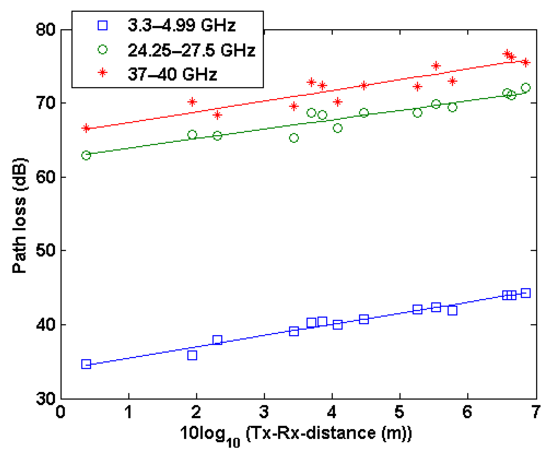
The 1-slope PL model has been also evaluated for the bands 3.3–4.99 GHz, 24.25–27.5 GHz and 37–40 GHz. Figure 7 presents the PL as a function of these three bands and the respective 1-slope models (PL index shown in

Table 5. 1-slope model for selected World Radio Conference (WRC) bands.

Band	n	L0 (dB)	σX (dB)	R2
3.3–4.99 GHz	1.51	34.00	0.47	0.97
24.25–27.5 GHz	1.28	62.59	0.84	0.90
37–40 GHz	1.43	65.95	1.16	0.85

). It is noteworthy that only 3 GHz of bandwidth was available for the 37–43.5 GHz band due to the maximum 40 GHz frequency measured in this contribution. The results indicate that even if both slope values are close, the PL index for the 37–40 GHz band is larger than that of the first band. Also, the PL for the second band is larger as expected with a 3.8 dB difference on average agreeing rather well with the 3.6 dB Free Space path loss.

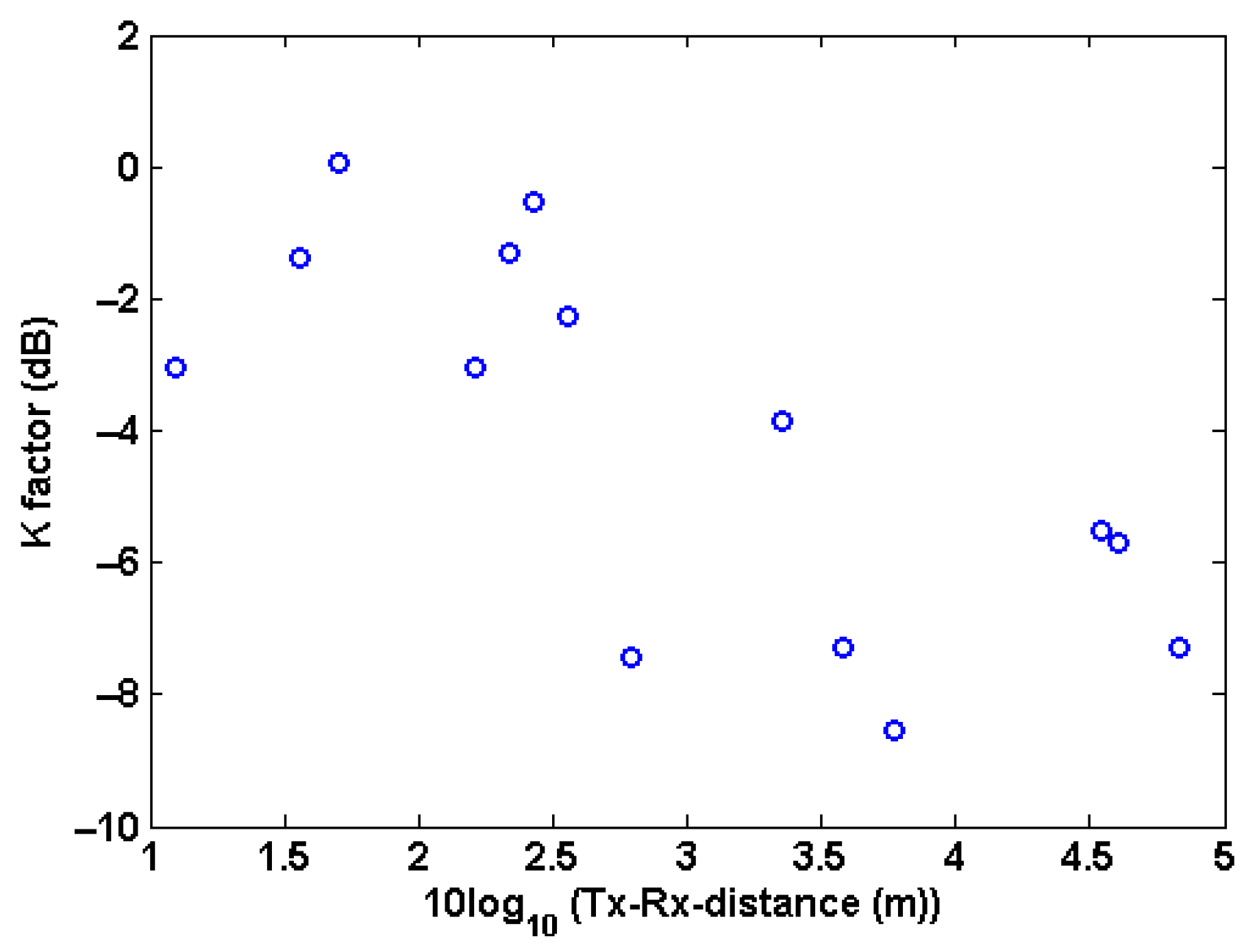
The K-factor has been computed as the quotient between the LoS component and the remaining energy; the K factor is shown in Figure 8.Negative values are measured, even in LoS situation due to the large number of contributions received (see PDP in Figure 4). This has also been observed in [19].

4. RMS Delay Spread

A wideband multipath channel can be described by its dispersion in the delay domain, which is usually expressed in terms of the RMS DS, ${\sigma }_{\tau }$. The RMS DS is defined as:

$${\sigma }_{\tau }=\sqrt{\frac{{\displaystyle \sum _{k}P({\tau }_k){\tau }_k^2}}{{\displaystyle \sum _{k}P({\tau }_k)}}-{\left(\frac{{\displaystyle \sum _{k}P({\tau }_k){\tau }_k^{}}}{{\displaystyle \sum _{k}P({\tau }_k)}}\right)}^2}.$$

(4)

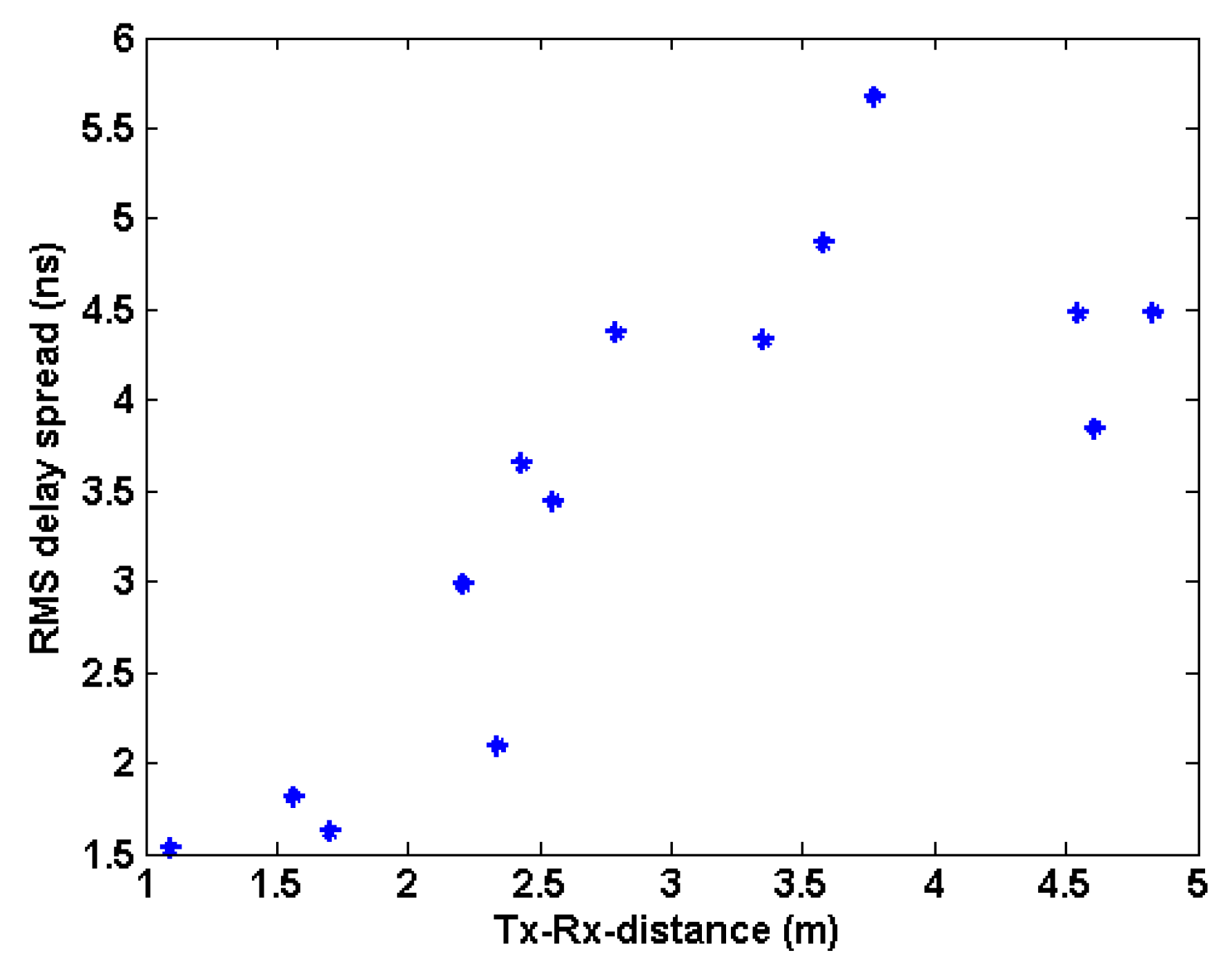
In Equation (4), τ_k are the delay values and P_k the PDP values in linear units. Figure 9 shows the RMS DS for a threshold of 30 dB, using the full bandwidth.

The RMS is observed to be increasing with distance, and as before, a simple 1-slope model can be derived:

$$DS=D{S}_0+10n_{DS}\times {\log }_{10}\left(d\right)+X\sigma \left(\mathrm{ns}\right),$$

(5)

where:

• DS₀ (in ns) and n_DS are adjustment parameters;
• d (in meters) is the distance between Tx and Rx, and
• X_σ (in ns), a Gaussian random variable with zero means and standard deviation σ (in dB).

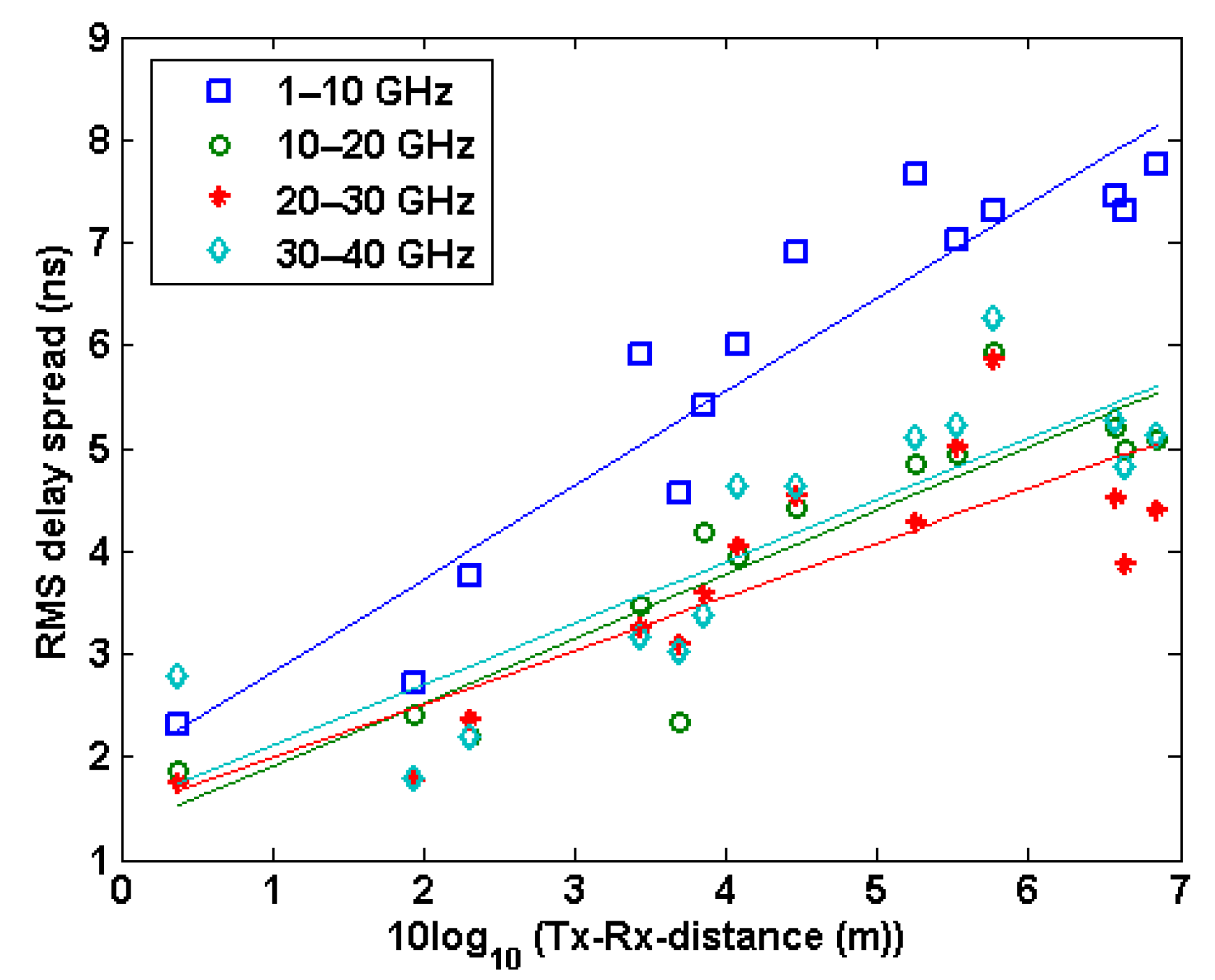
Figure 10 and

Table 6. 1-slope model for the root mean square (RMS) delay spread. The standard deviation and R² parameters of the linear model of Equation (5) are shown.

Band	nDS	DS0 (dB)	σX (dB)	R2
1–10 GHz	0.90	1.91	0.61	0.88
10–20 GHz	0.62	1.29	0.55	0.82
20–30 GHz	0.52	1.47	0.65	0.70
30–40 GHz	0.60	1.51	0.71	0.72

summarize the results for RMS DS at bands 1–10 GHz, 10–20 GHz, 20–30 GHz, and 30–40 GHz using a 30 dB threshold.

From Table 6 it is observed that the slope decreases with frequency. This effect is coherent with Figure 5 and the increase of attenuation of multipath components. The R² parameter shows a significative linear relation between the distance in logarithm units and RMS DS.

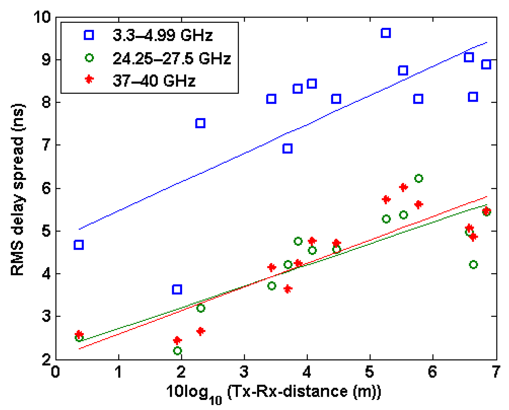
In addition, the RMS DS slope values for the selected WRC bands is shown in Figure 11, and tuned parameters in

Table 7. 1-slope model for the root mean square of the delay spread (RMS DS) for the selected WRC bands. The standard deviation and R² parameters of the linear model of Equation (5) are shown.

Band	nDS	DS0 (dB)	σX (dB)	R2
3.3–4.99 GHz	0.67	4.79	1.04	0.61
24.25–27.5 GHz	0.50	2.21	0.63	0.70
37–40 GHz	0.54	2.04	0.58	0.77

.

Usually, when the RMS DS is measured in several positions, its mean and standard deviation are obtained because they are two of the main parameters of the RMS DS’ statistical characterization. In

Table 8. Measured mean and standard deviation of the RMS DS. The measured values are compared with those found in the literature.

Band	Reference	RMS DS Mean (ns)	RMS DS Standard Deviation (ns)	Type of Environment
3.3–4.99 GHz	This work	7.71	1.66	Small office/lab.
24.25–27.5 GHz	This work	4.37	1.14	Small office/lab.
37–40 GHz	This work	4.42	1.20	Small office/lab.
26 GHz	[29]	16.08	2.18	Auditorium
28 GHz	[25]	17.20	16.40	Large office
	[28]	23.10	4.20	Industrial

, the mentioned parameters are shown for the WRC bands and they are compared with values found in the literature. To fairly compare the values of Table 8 the type of environment is also shown. As seen in Table 8, the mean and standard deviation of the RMS DS corresponding to large indoor environments, as large offices, industrial scenarios and auditoriums, are larger than the values found in a small open indoor environment, as the one measured in this work. This fact is due to the high number of large delay multipath components found in large rooms, whereas a fewer number of large delay components are present in smaller scenarios.

The multipath effect produces significant values of RMS DS which is one of the main factors that limit the system bit rate. Traditionally, the performance of the wireless system can be improved thanks to equalization algorithms; furthermore, the use of directional antennas along with circular polarizations can reduce the delay spread as indicated in [34].

5. Comparison with Ray-Tracing Simulations

5.1. Radio Channel Characteristics

A 3D ray-tracing tool (RT) has been programmed in MATLAB by our research group. The tool includes the usual reflected and diffracted components and combinations of them as well as single-order diffuse scattering components. The following mechanisms were considered in order to achieve a good accuracy and a reasonable simulation time: direct ray, up to two order reflections, simple diffractions, simple diffractions plus single reflections, single reflections plus simple diffractions and single order diffuse scattering components. The Lambertian model was used to simulate the diffuse scattering; this model has only one parameter, the scattering parameter S that controls how much energy is scattered in all directions [35]. An iterative method, as the one shown in [21], was applied to find the best values of the S parameter in the measured band and scenario. Moreover, the measured radiating pattern of the antennas (see Figure 3) were included to improve the accuracy in each path gain of all propagation mechanisms. In Figure 12 the comparison between the measured and simulated PDP for position 10 is shown; the 30 dB threshold is also depicted. As seen in Figure 12 the main groups of components, above the threshold, are correctly simulated by the ray tracing tool. As in the measurements, the Hanning window was used to extract the PDP.

In

Table 9. Comparison between the measured and simulated RMS of the DS between 1 GHz and 40 GHz.

Position	Simulated (ns)	Measured (ns)	Acc. (%)
1	2.99	4.51	66.27
2	3.41	3.86	88.28
3	3.53	4.39	80.43
4	3.30	5.85	56.45
5	3.53	5.02	70.42
6	3.35	4.28	78.12
7	3.11	3.25	95.66
8	3.57	4.04	88.33
9	2.83	4.53	62.63
10	2.21	3.58	61.64
11	1.73	2.36	73.22
12	0.99	1.74	56.61
13	1.58	3.09	51.15
14	1.78	1.78	100.0
-	-	Mean	73.50

, the comparison between the simulated and measured RMS DS is shown. A threshold of 30 dB was used in all cases. The results of the mean delay comparison are collected in

Table 10. Comparison between the measured and simulated mean delay between 1 GHz and 40 GHz.

Position	Simulated (ns)	Measured (ns)	Acc. (%)
1	16.20	17.32	93.51
2	17.06	17.32	98.46
3	18.44	18.57	99.30
4	14.46	16.35	88.44
5	13.36	14.94	89.49
6	12.35	13.07	94.47
7	8.14	8.36	97.34
8	9.76	9.94	98.15
9	11.45	10.95	95.43
10	8.05	9.19	87.60
11	5.59	6.17	90.60
12	3.67	3.87	94.65
13	7.92	8.52	92.92
14	5.29	5.52	95.75
-	-	Mean	94.00

. The mean accuracy of the RMS DS is close to 75%; the accuracy is below 60% for only three positions whereas the maximum accuracy is around 100%. The accuracy for the mean delay is high, reaching a mean value of 94.00%. A LoS component exists in all positions and the associated delay influences to a great extent the mean delay parameter. Since the LoS component is easily simulated with the ray-tracing tool, this explains the good match. Likewise, the PL accuracy is high as seen in

Table 11. Comparison between the measured and simulated PL between 1 GHz and 40 GHz.

Position	Simulated (ns)	Measured (ns)	Diff. (dB)
1	63.45	63.68	0.23
2	63.77	63.43	0.34
3	63.76	63.87	0.11
4	62.69	61.68	1.01
5	62.40	61.79	0.61
6	62.15	60.79	1.36
7	60.60	57.79	2.81
8	60.71	59.01	1.70
9	62.12	60.42	1.70
10	60.29	59.66	0.63
11	57.86	56.44	1.42
12	55.12	53.45	1.67
13	60.29	59.50	0.79
14	57.42	55.95	1.47
-	-	Mean	1.13

. As in Figure 5 the gain has been extracted from the simulated PL. The mean error in dB is only 1.13 dB. In general, the accuracy is high, it can be improved including higher order components are three and four-order reflections, multiple diffractions and even second-order diffuse scattering; the simulation of these components require large amounts of computer memory and they are also very time consuming; for these reasons higher order components were not included in this work.

The delay parameters and PL were also estimated using the simulated PDPs for the WRC’15/19 bands as presented in tables included in the Appendix A.

5.2. Propagation Mechanisms Analysis

In addition, the ray-tracing tool allows a comprehensive analysis of the significance of the included propagation mechanisms. For instance, the percentage of the simulated power of each one of the propagation mechanisms can be finely assessed as depicted in Figure 13. The antenna gain of transmitter and receiver of each path was not included to show only the channel effects.

Of course, the main propagation mechanism is the direct ray since all positions correspond to LoS situations. Apart from the direct ray, the main propagation mechanism is the reflection, although the diffraction represents an important percentage of the total power. The diffuse scattering power is smaller than the reflected and diffracted power, but it is still significant and increases with distance. The weaker mechanisms are those composed of a combination of a single reflection and a single diffraction.

The percentage of power of each propagation mechanism was also extracted for the WRC’15/19 as shown in Figure 14, Figure 15 and Figure 16 for the 3.3–4.99 GHz, 24.25–27.5 GHz, and 37–40 GHz bands, respectively. The results clearly demonstrate that the contribution of the LoS decreases with distance, whereas that of reflection and diffraction increases. This trend is clearly shown in all central frequencies. Furthermore, it can be observed that diffuse scattering is much less frequency dependent and should not be omitted when simulating low-mmW radio channels as reported in an earlier work at 60 GHz [32]. These results show that the radio channel becomes more simplistic at higher frequencies enabling the use of efficient simulation approaches such as ray-tracing.

6. Conclusions

In this work, we have presented MIMO experimental results on LoS data over the whole 1–40 GHz band in an 80 m³ office. Based on a VNA setup, measurements of the relative received power, PL, RMS DS and K-factor were extracted and compared with ray-tracing simulations to have an idea of how propagation behaves in all possible 5G frequency bands; the results obtained were compared to relevant results found in the literature. The decay factor of the PL behaves nearly constant with frequency whereas the slope of the RMS DS is quite sensible to frequency. The contribution of the propagation mechanisms is investigated using the simulated radio channels across the contiguous and 5G bands. Finally, the new WRC’15/19 5G bands are considered, and models are proposed for this scenario. In future works we will assess similar complete band analysis in other scenarios as outdoor and indoor to outdoor ones; the linear relation between the RMS DS and the transmitter-receiver distance in logarithmic units will be also thoroughly analyzed. Finally, a MIMO Rician model will be used to fit the measured data to achieve a deeper insight in the channel behavior.

References

1. Shafi, M.; Zhang, J.; Tataria, H.; Molisch, A.F.; Sun, S.; Rappaport, T.S.; Tufvesson, F.; Wu, S.; Kitao, K. Microwave vs. millimeter-wave propagation channels: Key differences and impact on 5G cellular systems. IEEE Commun. Mag. 2018, 56, 14–20. [Google Scholar] [CrossRef]
2. Cisco Visual Networking Index: Global Mobile Data Traffic Forecast Update, 2017–2022. February 2019. Available online: https://s3.amazonaws.com/media.mediapost.com/uploads/CiscoForecast.pdf (accessed on 28 July 2020).
3. IMT Traffic Estimates for the Years 2020 to 2030; ITU-R SG05; ITU: Geneva, Switzerland, July 2015.
4. Harris, P.; Malkowsky, S.; Vieira, J.; Bengtsson, E.L.; Tufvesson, F.; Hasan, W.B.; Liu, L.; Beach, M.; Armour, S.; Edfors, O. Performance characterization of a real-time massive MIMO system with LOS mobile channels. IEEE J. Sel. Areas Commun. 2017, 35, 1244–1253. [Google Scholar] [CrossRef] [Green Version]
5. Rossi, P.S.; Ciuonzo, D.; Kansanen, K.; Ekman, T. Performance analysis of energy detection for MIMO decision fusion in wireless sensor networks over arbitrary fading channels. IEEE Trans. Wirel. Commun. 2016, 15, 7794–7806. [Google Scholar] [CrossRef]
6. Ciuonzo, D.; Aubry, A.; Carotenuto, V. Rician MIMO channel- and jamming-aware decision fusion. IEEE Trans. Signal Process. 2017, 65, 3866–3880. [Google Scholar] [CrossRef] [Green Version]
7. Dey, I.; Rossi, P.S.; Butt, M.M.; Marchetti, N. Virtual MIMO wireless sensor networks: Propagation measurements and fusion performance. IEEE Trans. Antennas Propag. 2019, 67, 5555–5568. [Google Scholar] [CrossRef]
8. Duong, T.Q.; Chu, X.; Suraweera, H.A. The role of massive MIMO and small cells in ultra-dense networks. In Ultra-Dense Networks for 5G and Beyond: Modelling, Analysis, and Applications; Wiley: Hoboken, NJ, USA, 2019. [Google Scholar] [CrossRef]
9. Jungnickel, V.; Manolakis, K.; Zirwas, W.; Panzner, B.; Braun, V.; Lossow, M.; Sternad, M.; Apelfrojd, R.; Svensson, T. The role of small cells, coordinated multipoint, and massive MIMO in 5G. IEEE Commun. Mag. 2014, 52, 44–51. [Google Scholar] [CrossRef]
10. Proceedings of the World Radiocommunication Conference 2015 (WRC-15), Geneva, Switzerland, 2–27 November 2015; Available online: https://www.itu.int/en/ITU-R/conferences/wrc/2015/Pages/default.aspx (accessed on 28 July 2020).
11. Proceedings of the World Radiocommunication Conference 2019 (WRC-19), Sharm el-Sheikh, Egypt, 28 October–22 November 2019; Available online: https://www.itu.int/en/ITU-R/conferences/wrc/2019/Pages/default.aspx (accessed on 28 July 2020).
12. Rappaport, T.S.; Sun, S.; Mayzus, R.; Zhao, H.; Azar, Y.; Wang, K.; Wong, G.N.; Schulz, J.K.; Samimi, M.; Gutierrez, F. Millimeter wave mobile communications for 5G cellular: It will work! IEEE Access 2013, 1, 335–349. [Google Scholar] [CrossRef]
13. Hur, S.; Baek, S.; Kim, B.; Chang, Y.; Molisch, A.F.; Rappaport, T.S.; Haneda, K.; Park, J. Proposal on Millimeter-Wave Channel Modeling for 5G Cellular System. IEEE J. Sel. Top. Sign. Process. 2016, 10, 454–469. [Google Scholar] [CrossRef]
14. Rappaport, T.S.; Ben-Dor, E.; Murdock, J.N.; Qiao, Y. 38 GHz and 60 GHz angle-dependent propagation for cellular & peer-to-peer wireless communications. In Proceedings of the 2012 IEEE International Conference on Communications (ICC), Ottawa, ON, Canada, 10–15 June 2012; Institute of Electrical and Electronics Engineers (IEEE): Piscataway, NJ, USA, 2012; pp. 4568–4573. [Google Scholar]
15. Rappaport, T.S.; MacCartney, G.R.; Samimi, M.K.; Sun, S. Wideband millimeter-wave propagation measurements and channel models for future wireless communication system design. IEEE Trans. Commun. 2015, 63, 3029–3056. [Google Scholar] [CrossRef]
16. Hemadeh, I.A.; Satyanarayana, K.; El-Hajjar, M.; Hanzo, L. Millimeter-Wave Communications: Physical Channel Models, Design Considerations, Antenna Constructions, and Link-Budget. IEEE Commun. Surv. Tutorials 2018, 20, 870–913. [Google Scholar] [CrossRef] [Green Version]
17. Sasaki, M.; Yamada, W.; Sugiyama, T.; Mizoguchi, M.; Imai, T. Path loss characteristics at 800 MHz to 37 GHz in urban street microcell environment. In Proceedings of the 9th European Conference of Antennas and Propagation (EuCAP2015), Lisbon, Portugal, 12–17 April 2015. [Google Scholar]
18. Hejselbaek, J.; Karstensen, A.; Pedersen, G.F.; Hejselbak, J. Angular power distribution measurements and modelling of outdoor urban environment using ray-tracing at 2 and 18 GHz. In Proceedings of the 10th European Conference on Antennas and Propagation (EuCAP), Davos, Switzerland, 10–15 April 2016; pp. 1–5. [Google Scholar] [CrossRef] [Green Version]
19. Lee, J.-H.; Choi, J.-S.; Lee, J.-Y.; Kim, S.-C. 28 GHz Millimeter-wave channel models in urban microcell environment using three-dimensional ray tracing. IEEE Antennas Wirel. Propag. Lett. 2018, 17, 426–429. [Google Scholar] [CrossRef]
20. Hsiao, A.-Y.; Yang, C.-F.; Wang, T.-S.; Lin, I.; Liao, W.-J. Ray tracing simulations for millimeter wave propagation in 5G wireless communications. In Proceedings of the 2017 IEEE International Symposium on Antennas and Propagation & USNC/URSI National Radio Science Meeting, San Diego, CA, USA, 9–14 July 2017; pp. 1901–1902. [Google Scholar] [CrossRef]
21. Järveläinen, J.; Haneda, K. Sixty gigahertz indoor radio wave propagation prediction method based on full scattering model. Radio Sci. 2014, 49, 293–305. [Google Scholar] [CrossRef]
22. Study on Channel Model for Frequencies from 0.5 to 100 GHz; 3GPP TR 38.901 v14.2.0; European Telecommunications Standards Institute: Valbonne, France, September 2017.
23. Martinez-Ingles, M.; Pascual-García, J.; Gaillot, D.P.; Borras, C.S.; Molina-García-Pardo, J. Indoor 1-40 GHz channel measurements. In Proceedings of the 13th European Conference on Antennas and Propagation (EuCAP), Krakow, Poland, 31 March–5 April 2019; pp. 1–5. [Google Scholar]
24. Pimienta-del-Valle, D.; Hernández-Sáenz, S.; Sáiz-Coronado, P.; Mendo, L.; Garcia-del-Pino, P.; Riera, J.M. Indoor path loss measurements at the 5G millimeter-wave bands of 26 and 39 GHz. In Proceedings of the 13th European Conference on Antennas and Propagation (EuCAP), Krakow, Poland, 31 March–5 April 2019; pp. 1–5. [Google Scholar]
25. MacCartney, G.R.; Rappaport, T.S.; Sun, S.; Deng, S. Indoor office wideband millimeter-wave propagation measurements and channel models at 28 and 73 GHz for ultra-dense 5G wireless networks. IEEE Access 2015, 3, 2388–2424. [Google Scholar] [CrossRef]
26. Li, S.; Liu, Y.; Zhang, X.; Qi, X. Measurement and simulation of 28 GHz millimeter-wave propagation characteristics in the corridor environment. In Proceedings of the 2016 IEEE 9th UK-Europe-China Workshop on Millimetre Waves and Terahertz Technologies (UCMMT), Qingdao, China, 5–7 September 2016; pp. 134–137. [Google Scholar]
27. Tang, P.; Zhang, J.; Shafi, M.; Dmochwski, P.A.; Smith, P.J. Millimeter wave channel measurements and modelling in an indoor hotspot scenario at 28 GHz. In Proceedings of the 88th Vehicular Technology Conference (VTC-Fall), Chicago, IL, USA, 27–30 August 2018; pp. 1–5. [Google Scholar]
28. Schmieder, M.; Eichler, T.; Wittig, S.; Peter, M.; Keusgen, W. Measurement and characterization of an indoor industrial environment at 3.7 and 28 GHz. In Proceedings of the 2020 14th European Conference on Antennas and Propagation (EuCAP), Copenhagen, Denmark, 15–20 March 2020; pp. 1–5. [Google Scholar] [CrossRef]
29. Ai, B.; Guan, K.; He, R.; Li, J.; Li, G.; He, D.; Zhong, Z.; Huq, K.M.S. On indoor millimeter wave massive mimo channels: Measurement and simulation. IEEE J. Sel. Areas Commun. 2017, 35, 1678–1690. [Google Scholar] [CrossRef]
30. Available online: http://emcore.com/products/optiva-ots-2-series-microwave-band-50-mhz-to-40-ghz-fiber-optic-links/ (accessed on 28 July 2020).
31. Available online: https://www.steatite-antennas.co.uk/wp-content/uploads/2017/09/QOM-SL-0.8-40-K-SG-L.pdf (accessed on 28 July 2020).
32. Martinez-Ingles, M.; Gaillot, D.P.; Pascual-Garcia, J.; Molina-Garcia-Pardo, J.; Lienard, M.; Rodríguez, J. Deterministic and experimental indoor mmW channel modeling. IEEE Antennas Wirel. Propag. Lett. 2014, 13, 1047–1050. [Google Scholar] [CrossRef]
33. mmMAGIC. Measurement Results and Final mmMAGIC Channel Models. H2020-ICT-671650-mmMAGIC/D2.2 v2.0. 2017. Available online: https://5g-mmmagic.eu/results/ (accessed on 29 July 2020).
34. Haneda, K. Channel models and beamforming at millimeter-wave frequency bands. IEICE Trans. Commun. 2015, E98-B, 755–772. [Google Scholar] [CrossRef] [Green Version]
35. Degli-Esposti, V.; Fuschini, F.; Vitucci, E.M.; Falciasecca, G. Measurement and modelling of scattering from buildings. IEEE Trans. Antennas Propag. 2007, 55, 143–153. [Google Scholar] [CrossRef]
Figure 1. Photo of the measurement scenario.
Electronics 09 01688 g001
Figure 2. Map of the measurements.
Electronics 09 01688 g002
Figure 3. Measured antenna pattern in dB for different frequencies.
Electronics 09 01688 g003
Figure 4. The power delay profile (PDP) for position number 10 of Figure 2.
Electronics 09 01688 g004
Figure 5. Measured path loss (PL) using all bandwidth, line-of-sight (LoS) PL, and Friis model. The antenna effect has been subtracted from the measured values.
Electronics 09 01688 g005
Figure 6. PL for the bands and their 1-slope models.
Electronics 09 01688 g006
Figure 7. PL for the World Radio Conference (WRC) bands and their 1-slope models.
Electronics 09 01688 g007
Figure 8. Measured K-factor.
Electronics 09 01688 g008
Figure 9. Full bandwidth root mean square of the delay spread (RMS DS) versus the Tx-Rx distance in logarithm units.
Electronics 09 01688 g009
Figure 10. RMS DS at 5 GHz, 15 GHz, 25 GHz, 35 GHz central frequencies versus the Tx-Rx distance in logarithmic units.
Electronics 09 01688 g010
Figure 11. WRC bands RMS DS versus the Tx-Rx distance in logarithmic units.
Electronics 09 01688 g011
Figure 12. Comparison between the measured and simulated PDP for position number 10.
Electronics 09 01688 g012
Figure 13. Percentage of power of different propagation mechanisms for all positions when the frequency is 20.5 GHz.
Electronics 09 01688 g013
Figure 14. Percentage of power of different propagation mechanisms for all positions when the frequency is 4.145 GHz, central frequency of the band 3.3–4.99 GHz.
Electronics 09 01688 g014
Figure 15. Percentage of power of different propagation mechanisms for all positions when the frequency is 25.875 GHz, central frequency of the band 24.25–27.5 GHz.
Electronics 09 01688 g015
Figure 16. Percentage of power of different propagation mechanisms for all positions when the frequency is 38.50 GHz, central frequency of the band 37–40 GHz.
Electronics 09 01688 g016