Spatio-Temporal Distribution of Carabids Influenced by Small-Scale Admixture of Oak Trees in Pine Stands

Department of Forest Sciences, Faculty of Environmental Sciences, Institute of Silviculture and Forest Protection, TU Dresden, 01737 Tharandt, Germany
*
Author to whom correspondence should be addressed.
Diversity 2020, 12(10), 398; https://doi.org/10.3390/d12100398
Submission received: 10 August 2020
/
Revised: 26 September 2020
/
Accepted: 14 October 2020
/
Published: 15 October 2020
(This article belongs to the Special Issue Interactions between Oaks and Insects)
Abstract
:In a region with poor soil fertility, low annual precipitation and large areas of homogenous Pinus sylvestris L. forests, conservation of old sessile oak (Quercus petraea (Matt.) Liebl.) trees is one option to enrich structure and species richness. We studied the affinities of Carabus coriaceus, C. violaceus, C. hortensis and C. arvensis for specific tree species and the resultant intra- and interspecific interactions. We focused on their temporal and spatial distributions. Pitfall traps were used as a surface-related capture method on a grid over an area of three hectares. Generalised linear models and generalised linear geostatistical models were used to analyse carabid activity densities related to distance-dependent spatial effects corresponding to tree zones (oak, oak–pine, pine). The results demonstrated significant spatial affinities among these carabids, especially for females and during the period of highest activity. Individuals of C. coriaceus showed a tendency to the oak zone and C. hortensis exhibited a significant affinity to the oak–pine mixture. Imagines of C. arvensis and C. violaceus were more closely related to pine. The observed temporal and spatial coexistence of the different Carabus species reveals that single admixed old oak trees can support greater diversity within pine-dominated forests.
1. Introduction
Forest ecosystem management in central Europe aims to preserve or increase the level of structural and species biodiversity, especially in forests previously managed primarily for wood production and consisting predominantly of Norway spruce or Scots pine [1]. It has been highlighted in recent decades that the decline of biodiversity in forest ecosystems has fundamental consequences for many genera, also for insects [2]. The importance of tree species and structural diversity for insects has been shown for several types of forest ecosystem [3,4,5,6]. Therefore, most forest management activities in even-aged coniferous forests target a timely establishment of site-specific deciduous tree species admixtures of different ages, forms and proportions; for example, by means of forest conversion [7,8]. However, the ecological effects exerted by existing single-tree admixtures within these homogeneous forests are often overlooked by current inventory systems given their low relevance in economic terms [9,10]. Numerous studies have demonstrated the establishment of diverse ecological niches for different groups of species as created, in particular, by single trees or groups of old oak or beech trees within homogeneous coniferous forests [11,12,13]. The ecological assessment of single-tree admixtures is even more important for landscapes with a homogenous topography, less favourable site conditions (poor in nutrients with low precipitation) and a long-term dominance of one tree species over large areas than is the case in more diverse landscapes. Conditions lacking diversity are characteristic of the eastern part of the German lowlands, which are dominated by single-layered Scots pine (Pinus sylvestris L.) forests, not least because of the limited range of naturally site-specific deciduous tree species. Sessile oak (Quercus petraea (Matt.) Liebl.) is one of the tree species that occurs naturally in this region in a mixture with pine, and is known for a high number of associated groups of insects [14,15].
The basic effects of oak–pine mixtures have been studied mainly with a focus on growth interactions between these tree species [16,17], the effects for humus and soil conditions [18,19,20], and on regeneration [21]. Most insect studies in relation to oak and pine mixtures compared the presence, abundance or richness of species between pure and mixed forests [3,22,23]. In pine forests, the quality and quantity of ecological effects (biotic or abiotic) produced by admixed oak trees depend on individual tree traits, for example, age and stem or crown dimension [13,20,22]. Individually admixed oak trees primarily determine the small-scale habitat conditions relevant for faunal species within the direct surroundings by modifying, for example, the availability and spatial distribution of light, temperature, water and nutrients [20,24]. Previous studies described the decrease in the effect exerted by oak trees with increasing distance from the tree. Starting from the oak zone, a smooth transition to a smaller zone of ‘strongly mixed effects’ intensively influenced by both oak and pine, followed by zones mainly affected by pine trees [25,26]. The proportion of strongly mixed effect zones causing edge effects within a defined forest area depend on the intensity and form of tree species mixtures (single trees versus tree groups). Oak and pine tree mixtures create varied microhabitat patches of contrasting suitability for soil-dwelling insects [27].
The availability of spatially explicit information would promote an actively optimised and more efficient arrangement of mixed forests on different spatial scales [28]. Extensive experience has been gleaned in the theoretical background to single tree-based studies represented by different model approaches [29]. However, such results cannot be directly transferred to higher spatial levels like large forest or landscape areas [30]. The use of spatial (geo)statistical models allows for linkage of spatial information pertaining to trees or forests and their effects on mobile species like insects [13,31,32]. The position-dependent spatial effects of an individual tree, for example, the impact on the light or water regime, or the dispersal of leaves in autumn, are strongly influenced by the individual lifespan of this tree and its species-specific tree attributes like crown dimension [26,33,34]. For spatially explicit analyses it is important that all of the effects of individual trees, direct or indirect, are linked with their position within a defined environmental matrix. However, spatial analyses of faunal species are also characterised by spatial data resulting from species behaviour and locomotory systems strongly influenced by environmental conditions. These processes of movement lead to species-specific differences in spatial activity densities and distributions that are difficult to predict [35]. Yet prediction is necessary to establish appropriate sample methods linked to forest structures. The evaluation and quantification of movements of Carabus beetles are especially difficult, because comprehensive knowledge of the species’ behaviour is necessary and in previous studies often only coarse stratifications of environmental structures like landscape elements were used, for example, forest versus open field [36,37,38]. Consequently, the combination of spatial tree effects and the spatial dynamics of mobile species constitutes a particular challenge. This is caused by the overlying effects of species-specific behavioural patterns (e.g., intrinsic and extrinsic motivations) [39,40]. To assess this approach, we selected four flightless Carabus species, given the availability of species-specific information about (i) their seasonal behaviour, (ii) their selection of different habitat structures and (iii) their classification as potential environmental indicators [30,39,41,42,43,44]. Previous entomological studies in forest ecosystems characterised Carabus coriaceus (L. 1758) as more widely present in deciduous forests than Carabus violaceus (L. 1758) and Carabus arvensis (Hbst. 1784), which were described as being more frequent in coniferous forests [45,46]. The analyses of the forest habitat preferences of Carabus hortensis (L. 1758) showed a stronger adaptation to habitat conditions influenced by admixtures of deciduous and coniferous tree species [46].
The behaviour of Carabus species is also affected by the temporal dimension, which includes seasonal variations of climate conditions and specific metamorphic behaviour, for example, periods of food-search, mating or oviposition [39,47,48,49]. It can be assumed that the combination of environmental factors relevant for temporal and spatial environmental dimensions have an impact on further behavioural Carabus interactions such as coexistence or competition on micro-scales [40,41,42,43,44,45,46,47,48,49,50,51,52,53]. These interaction principles are an integral part of Hutchinson’s concept of ecological niches [47,54,55]. By following this research approach, we explicitly combined temporal and spatial analyses of single admixed oak trees in pine-dominated forests with different degrees of relevance for the aforementioned Carabus species.
The research was based on the following hypotheses:
- Local climate conditions like temperature and precipitation significantly influence species-specific activity densities over the course of the year and the main period of activity (May to August) of the four Carabus species in pine-dominated forests.
- The spatial distribution patterns of Carabus species (interspecific) and sexes (intraspecific) are determined by the following spatial tree species effect zones: pure oak effect zone (Z1), mixed oak–pine effect zone (Z2) and pure pine effect zone (Z3).
- The combination of temporal (annual periods with high versus low activity densities) and spatial dimensions (small-scale tree species effect zones) leads to more detailed information about the species-specific use of environmental niches and helps to prove the derived assumptions of coexistence or intra- and interspecific competition of Carabus species [39,53].
2. Materials and Methods
2.1. Study Area
The study area of approx. 3 ha is located in the German Federal State Brandenburg, in the German lowlands (51°47′09.69″ N, 13°34′00.32″ E). The elevation above sea level is 64 m. The poor and sandy soil conditions are typical for this region. The whole forest area is dominated (98 %) by single-layered Scots pine stands of two ages, 36 and 61 years. The Scots pine trees have mean heights between 14.1 and 19.5 m and mean diameters at breast height (dbh) of 16.2 and 24.4 cm, respectively. The number of single admixed sessile oak trees is 31 (randomly distributed, Figure 1). These oak trees are aged between 70 and 150 years with a mean dbh of 26.6 cm and a mean height of 14.8 m. The mean crown dimensions of the admixed oak trees are 11.5 m in length and 7.2 m in diameter. The moss layer of the ground vegetation is dominated by Hypnum spp. and Pleurozium schreberi (Brid.), whereas the herb and shrub layers exhibit a high abundance of Deschampsia flexuosa (L.), Vaccinium myrtillus (L.) and Vaccinium vitis-idaea (L.). The proportion of oak occurring naturally in these pine forests would be higher based on the potential natural vegetation [56].
2.2. Climate Data
The climate conditions of this north-eastern region of the German lowlands are slightly continental. During the three years of measurements (2010 to 2012), the regional climate was characterised by mean annual temperatures of 8 °C, 10 °C and 9.5 °C, respectively. The total annual precipitation reached 710 mm (2010), 630 mm (2011) and 568 mm (2012) [57]. Additional local climate information is available from a professional climate monitoring station located in a pine forest approx. 1 km from the study area [58]. The local climate data were used to test the possible effects of air and soil temperature and total precipitation on the behaviour and movement of the selected Carabus species considering the periods with high and low activity (Table 1, Figure 2). Linear regressions (y = a·bx, p-value ≤ 0.05) were used to analyse the effects of mean soil surface temperatures and total precipitation for the activity densities of the Carabus species.
2.3. Measurements and Sample Design
Employing a capture-recapture method, the Carabus species were sampled using 123 dry and unbaited pitfall traps (diameter 7.5 cm, depth 9 cm) on a grid of 15 m × 15 m to cover the whole study area of 3 ha [26]. The capture-recapture method (also known as the mark–release–recapture method) is a gentle method to catch beetles alive, mark them individually and release them. This method is used to obtain information relevant for populations; for example, sex ratios, activity densities and spatial distributions of Carabus species [59]. All pitfall traps were clearly defined according to their spatial x- and y-coordinates. For the calculation of x- and y-coordinates (Cartesian coordinates) for all traps and trees we used polar coordinates measured by a laser-dendrometer (type LEDHA-GEO 100) with a precision of 0.5° for the direction and of 0.1 m for distances. To compute the activity densities of Carabus species, the density of individuals per trap was taken as being representative of the density per m2 and for the area surrounding each trap [39]. The term activity density describes the number of individuals per unit of area in entomology [60]. The interval of control for the pitfall traps was 1 to 3 days for the period from August 2010 to May 2012, with an interruption in January and February of 2011. The control interval should be no longer than 3 days to reduce stress for the trapped beetles. The traps were also filled with cones, branches and mosses for the same reason. The mean activity densities for each Carabus species were aggregated to monthly values to follow their course over the year. This monthly resolution of the activity densities for the Carabus species allowed for a separation of the intrinsically (factors like intraspecific interactions, territoriality) and extrinsically (abiotic factors, interspecific interactions) controlled activity densities [61,62], known as species-specific periods with primary (high activity: May to September) and secondary (low activity: October to April) importance of activity [63,64]. We aggregated the sampled carabids into these two temporal periods for further statistical analyses, because smaller temporal intervals would have resulted in overly low numbers of samples. Variation in behaviour over time is highly influenced by intrinsic motivations such as reproduction and the search for food. Species-specific interruptions to activity are known and referred to as different types of ‘diapause’ or ‘dormancy’ [39,48,64], which are strongly determined by life-cycles (phenology). The sex (females versus males) of all individuals of the four Carabus species (C. coriaceus, C. violaceus, C. hortensis, C. arvensis) was recorded, all were marked individually and re-released approx. 1.5 m from the trap in which they were caught [65]. The re-release distance from the trap was used to reduce the probability of an immediate recapture of the same beetle caused by the proximity to the trap.
To address spatially explicit single-tree effects in relation to the spatial activity densities of the four Carabus species, the stems of all trees (Scots pine: n = 2707, sessile oak: n = 31) were mapped (Figure 1). Three different spatial zones of distance-dependent influence of single oak trees were defined [26,66]. The first zone (Z1) describes the distance between the oak trunk and the crown edge projection (Z1: 0 m to <4 m), representing the area directly covered by oak crowns. The environmental conditions within the second zone (Z2) are characterised by ‘strongly mixed forest conditions’ attributed to the oaks and pines (Z2: ≥4 m to 15 m), because of the equal exertion of effects by trees of both species and the resultant mixture of oak and pine litter. The third zone (Z3) is representative of the pure pine parts of the study area (Z3: ≥15 m to 30 m). The overall proportions of the three zones over the whole study area were as follows: Z1: 4.9%, Z2: 33.3% and Z3: 62.8%.
2.4. Preparation of Spatial Data and Statistical Analyses
To apply generalised linear models (glm) and generalised linear geostatistical models (glgm) we computed all minimum distances between oak trees and each pitfall trap and assigned one of the effect zones ‘oak’ (Z1), ‘mixed’ (Z2) or ‘pine’ (Z3) to each trap (Figure 1) [67]. The number of beetles in the traps, that is, the beetle activity density, was approximately negative-binomially distributed. Therefore, we applied the models for negative-binomially distributed data to test for effects of species, sex and effect zone on beetle activity density.
As the traps were organised in a grid (see above), a general assumption of independence of individual trap data had to be investigated. To do so, we tested model residuals (qq-plots), heteroscedasticity in the residuals, and we checked for spatial autocorrelation of residuals by computing semi-variograms (see Figures S1 and S2). Although these semi-variograms showed no tendency towards spatial autocorrelation, we applied generalised linear geostatistical models (glgm) as an additional option for the analyses of spatial data. For examples of model applications with entomological data see, for instance, [31,32]. Within R (version 3.6.1; R Core Team 2019) the functions ‘glm.nb’ (package ‘MASS’) and ‘glgm’ (package ‘geostatsp’, [68] were used; the latter fits non-Gaussian models using INLA (version 1.7.4). The INLA procedure performs a wide range of Bayesian statistical analyses by applying sophisticated approximations to handle the numerical difficulties that commonly arise in this context [69].
The glm model in the case of sex (intraspecific) and effect zone effects was formulated as follows:
with AD as activity density and,
When testing for species (interspecific) and effect zone effects, the species were assigned factorial levels as follows:
To run the generalised linear geostatistical models, we followed a procedure described in detail [70]. Starting from suitable prior distributions, we obtained approximate posterior distributions and credible intervals ([71], Section 5.5). Although the interpretation of the credible interval differs from true confidence intervals, one may state that a parameter is significant if the 0.95-credible interval with endpoints defined by the 0.025th and 0.975th quantiles of the posterior distribution does not include 0. In Bayesian statistics, the credible interval does not refer to the hypothetical distribution assuming the parameter is exactly 0, which typically has zero probability under the prior distributions, but instead means the deviations manifesting themselves in the data are so significant that there is at least a 97.5 % chance of drawing the correct conclusion about whether the parameter is greater than or less than 0.
A general question in the Bayesian context concerns the robustness of the results against possible misspecifications of the priors ([72], Section 4.7), particularly if there is little prior knowledge. In our case, the only critical parameter was the standard deviation σ (or the precision 1/σ2). Therefore, we repeated our computations with a broad range of plausible priors for σ and yielded different corresponding posterior distributions. This means care should be taken when interpreting the statistical results and, in particular, that it is necessary to avoid attaching too much meaning to precise numerical values.
The estimation of the range [73] and standard deviation of the random part of the model was performed during the fitting procedure. The range was estimated by establishing a variogram. The standard deviation σ measured the strength of the spatial random effects.
The temporal distribution of the four Carabus species’ densities was tested using the ‘adonis’ function of the R-package ‘vegan’ [74] to make sure that the temporal activity of the chosen Carabus species was similar, and that the subdivision into the two main periods of ‘high activity’ and ‘low activity’ was usable.
3. Results
3.1. Temporal Activities of Carabus Species Influenced by Temperature and Precipitation
The sex ratio indicated higher proportions of males than females for C. coriaceus (1.78), C. violaceus (1.50) and C. hortensis (1.79). In the case of C. arvensis there was a higher proportion of females (0.91). The overall results of the activity densities during 2010 and 2012 proved higher densities for males than females, which were significant for C. coriaceus, C. violaceus and C. hortensis. The highest activity densities for the entire sample period were recorded for males of C. arvensis and C. coriaceus with 1.34 and 1.17 individuals per m2, respectively. For all four Carabus species the period of high activity extended from May to September, whereas low activity was registered between October and May. The highest activity densities of imagines were recorded in August 2011 for C. violaceus (1.94 ind. per month·m2) and C. coriaceus (1.36 ind. per month·m2), whereas C. arvensis (1.71 ind. per month·m2) and C. hortensis (0.39 ind. per month·m2) reached highest activity densities in May 2011. Months with high activity densities for females and males were coincidental on the species level, but revealed fluctuations between species (Table 1). The main activity period for females of C. coriaceus was observed between May and October. None of the observed Carabus species were present during the winter period between November and March, during which time mean surface temperatures were less than 5 °C. The permutational test revealed that the four Carabus species exhibited comparable temporal activity without significant differences (r-square for Carabus species = 0.323, p-value = 0.583, f.model = 0.954).
Based on the assumption that climate conditions determine the periods of carabid activity [39], we analysed the influence of monthly soil surface temperature and total precipitation. The contour lines in Figure 2 indicate the overall occurrence with activity densities more than 0.1 individuals per m2 at soil surface temperatures higher than 7.5 °C, but for a broad range in the quantity of precipitation. The relationship between mean soil surface temperature and activity densities could be described significantly by positive regressions (p-value ≤ 0.05) for all four Carabus species. This was not the case for the amount of precipitation. The lowest recorded monthly temperature when individuals of C. arvensis were active was 10 °C in April 2012. C. coriaceus and C. hortensis ended their activity period at 9.4 °C in October 2010, whereas C. violaceus was only active at mean monthly temperatures of more than 14 °C. A coherent activity period (May to August/September) was observed for both sexes of C. violaceus, with a maximum activity density during August with the highest mean monthly soil surface temperatures of 19 °C. The highest activity densities for C. coriaceus and C. violaceus were measured in August 2012, at a temperature of 19 °C. In comparison, C. hortensis and C. arvensis already reached their highest activity densities in May in 2011, at a temperature of 14.8 °C. Sex-specific differences in relation to the amount of precipitation were obvious for C. coriaceus. Figure 2 underlines that females of C. coriaceus were present to a higher degree during periods with higher precipitation (>120 mm), whereas males tended to favour lower amounts of precipitation (<100 mm). The highest activity densities of C. coriaceus males were recorded in months with 40–80 mm total precipitation.
3.2. Intraspecific Spatial Distribution Pattern of Carabids
A tendency towards a preference for the oak zone was revealed for C. coriaceus over the whole sample period 2010–2012 and especially for the period of low activity (Z1: 1.035, p-value ≤ 0.1; Table 2, Figure 3). This trend was also observed for females of C. hortensis, but was not shown to be significant by the results of the generalised linear model. A significant preference for the oak-pine zone was revealed for individuals of C. hortensis over the whole period of observation 2010–2012 (Z2: 1.223, p-value ≤ 0.01) and particularly for the period of high activity (Z2: 1.310, p-value ≤ 0.05), but not for the period of low activity (Table 2, Figure 3). Both sexes of C. violaceus had high activity densities within Z2 and Z3. There was a stronger tendency to Z3 for males than for females, but not significantly so. No effect of the interaction between zone and sex was detected for any species.
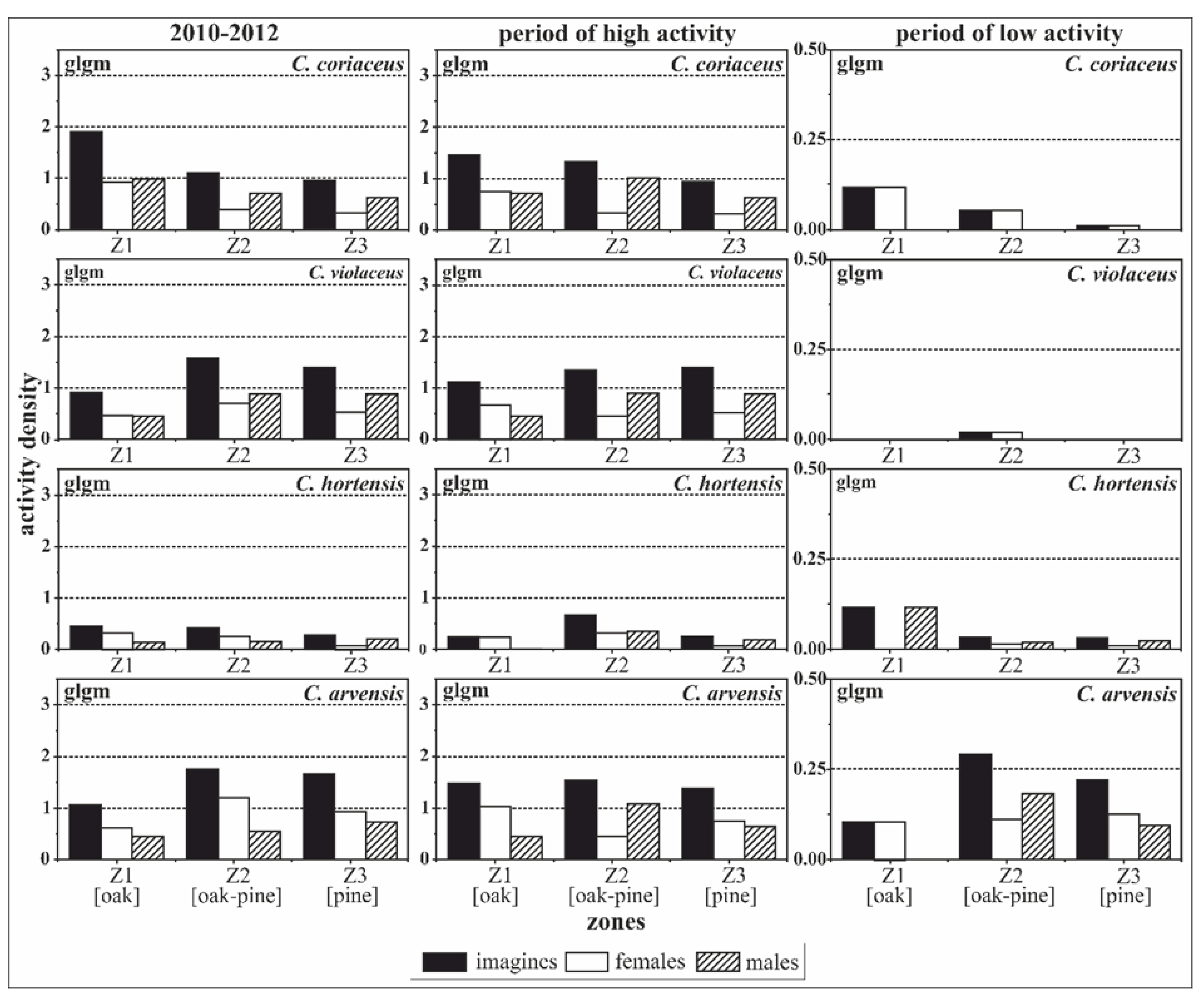
All of the results of the spatial analyses comparing the sexes and zones during the different periods and based on the generalised linear models (glm) were confirmed by the generalised linear geostatistical model (glgm) calculations (Table 3, Figure 4). However, the effects were found to be less significant in the geostatistical model.
3.3. Interspecific Spatial Distribution Patterns of Carabids
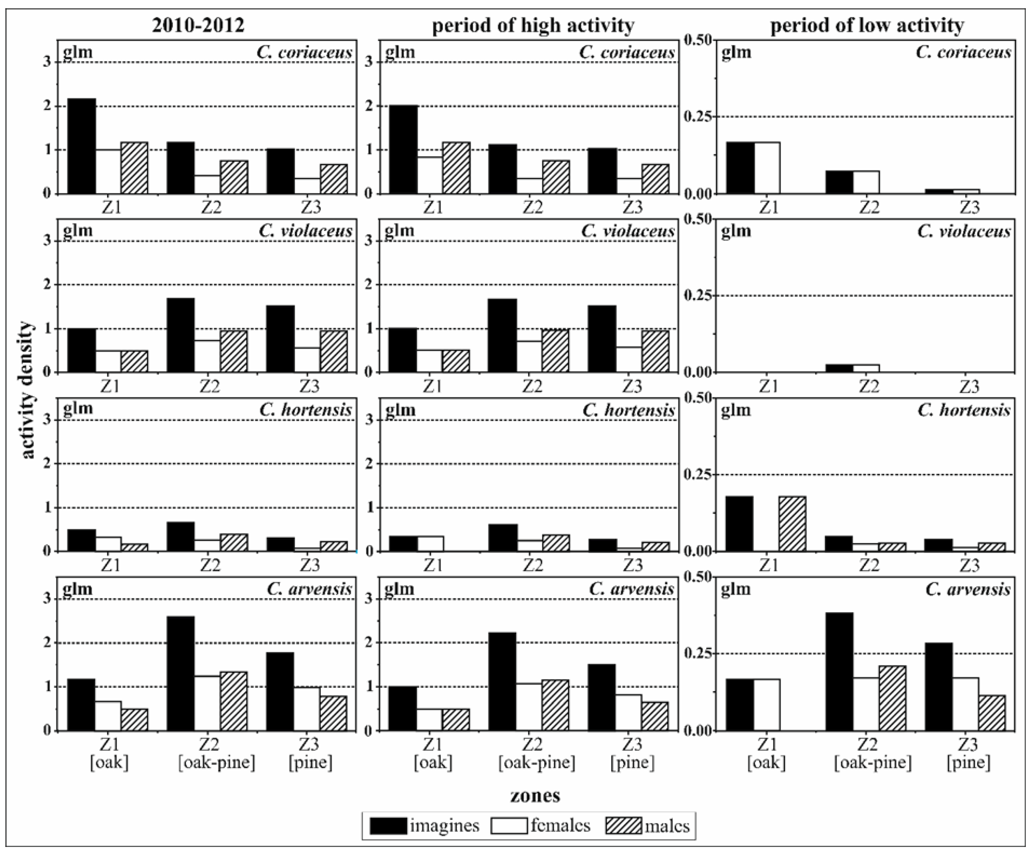
The comparison between the four Carabus species underlined significant differences in the total activity densities of imagines and of females, in particular for the periods 2010 to 2012 and during periods of high activity (Table 4 and Figure 5). However, the overall activity densities of males were similar for C. coriaceus, C. violaceus and C. arvensis; with the exception of the significantly lower activity densities of C. hortensis (Table 4, −1.099, p ≤ 0.001). The males of the four Carabus species exhibited no significant differences in activity density in relation to the zones during the two periods of activity.
A significantly higher activity density was evident in the oak zone (Z1) for females. The parameters in Table 4 emphasise the tendency towards a negative interaction of C. violaceus and C. arvensis imagines in the pure oak zone (Z1), especially over the whole period of observation 2010–2012 (−1.161 for C. violaceus, −1.168 for C. arvensis, p ≤ 0.1) and for the period of high activity. In C. hortensis a significant positive tendency towards the oak–pine mixed zone (Z2) was revealed for imagines and females during 2010–2012 overall (0.646, imagines p ≤ 0.1 and 1.069, females p ≤ 0.1) and for the period of high activity (0.760, imagines p ≤ 0.1 and 1.312, females p ≤ 0.05).
4. Discussion
4.1. Effects of Climate Conditions on the Temporal Activity of Carabids
The results validated the observation of species-specific periodicity of activity, which depends on life cycle processes such as breeding periods [75], but also on seasonal environmental conditions occurring at local scales [47]. While soil surface temperatures were directly related to activity densities, it was difficult to determine species-specific activity densities for all four species on the basis of the amount of monthly precipitation. Szujecki [76], for example, found that C. arvensis is theoretically present in a broad range of biotopes with different humidity conditions (Figure 2). Although mixed forests are characterised by more humid habitat conditions, this would probably not lead to higher densities of C. arvensis individuals. Studies focused solely on the effect of climate conditions over time should use higher time resolutions, for example, measurable by time-sorting pitfall traps [77]. To link the spatial distribution of carabids and climate parameters it is also necessary to use a small-scale resolution for climate data.
Low temperatures are a clear cause of low activity densities in Carabus species [39,46], and the hibernation of adults as part of the life cycle explains the complete absence of individuals during this period [78]. Our data confirmed that C. arvensis is spring active [46] and that C. coriaceus and C. violaceus are species with high levels of autumn activity [75,79] (Table 1).
Both sexes of C. arvensis showed the earliest (April) and most continuous presence during the year compared to the other species. Mean soil surface temperatures of approximately 10–12 °C were identified as a climatic trigger for increasing activity density in both sexes of C. arvensis. Due to the low number of total activity densities, it is difficult to verify an assumption for C. hortensis. Although C. hortensis also exhibited early activity in April, a diapause was noted for this species, with a minimum activity density in July despite soil surface temperatures of 18–19 °C. This seasonality independent of temperature is similar to the results documented by Elek et al. [79], who characterised C. hortensis as being constant in the seasonal chronology without differences along environmental gradients. One further explanation for the diapause during months of optimal temperatures may derive from the fact that C. hortensis is characterised as being night active and in the study region there are only a few hours of darkness each day between mid-May and the end of July [80,81,82]. The high densities of C. coriaceus were strongly related to soil surface temperatures of approx. 19 °C, with activity starting at 9 °C. For individuals of C. coriaceus the first activities start from a temperature of 14.1 °C and 17 °C, respectively [83,84]. According to the precipitation-dependent activity densities, C. coriaceus can be characterised as a meso-hygrophilous Carabus species within forest ecosystems [85,86]. The monthly activity density of C. violaceus individuals followed a sharp rise related to soil surface temperatures above 15 °C up to 20 °C, which compared with the results of Thiele and Weber [84], who documented a temperature range of activity from 15–21 °C. The contour lines almost parallel to the axis of precipitation in Figure 2 confirm small effects of the amount of precipitation on the activity densities of C. violaceus. A tendency towards a positive relationship between humidity and activity density has been observed for this species [87], with a strong response to air humidity levels of 85–97% described. However, our data did not demonstrate a statistically significant positive relationship.
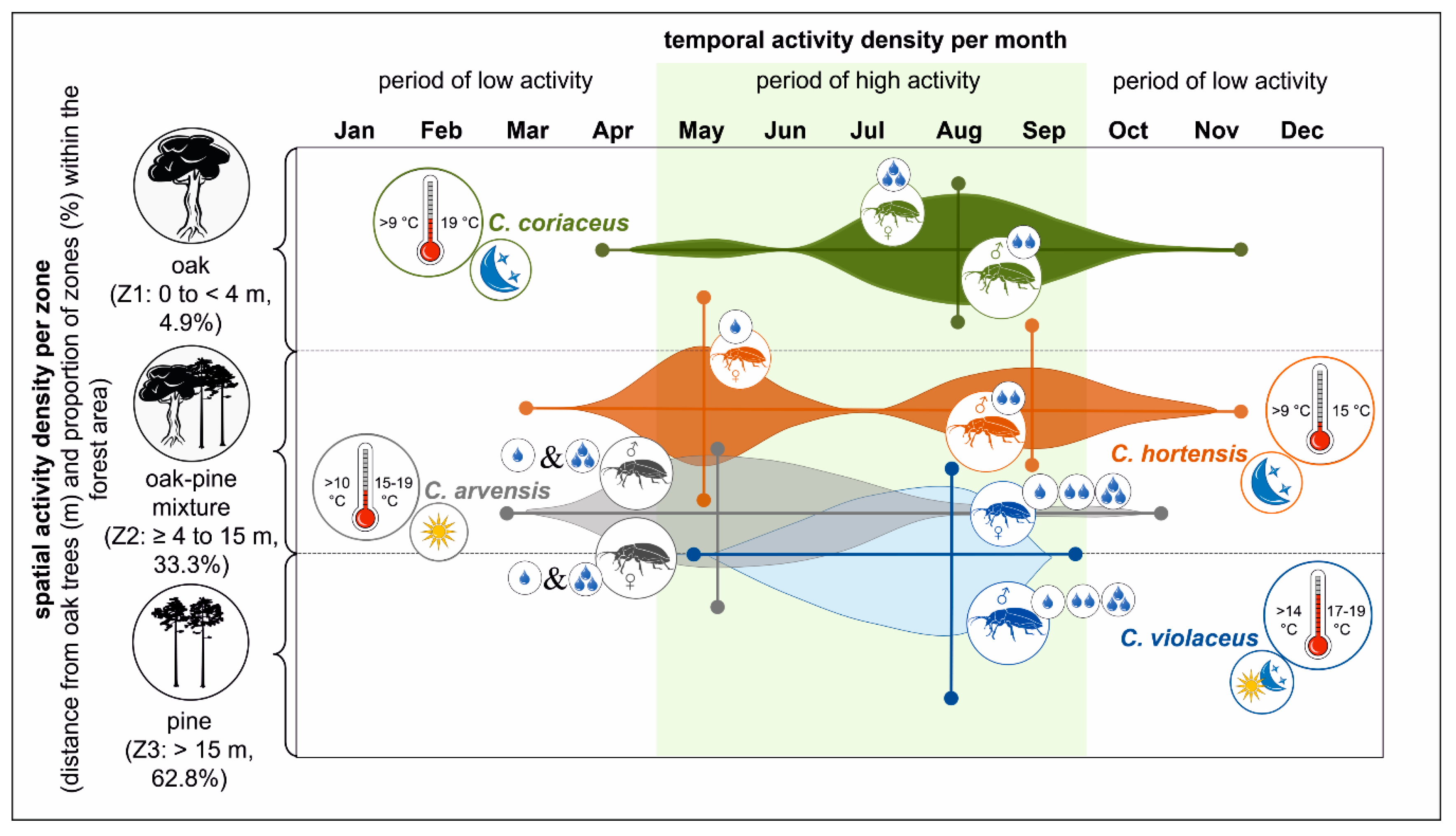
In spite of some overlaps in the timing of activity periods for the four Carabus species, the temporal dynamic differed in terms of (i) the overall duration of the activity period, (ii) the months with highest activity densities and (iii) the presence of dormancy (Figure 7). Minimum temporal overlaps in the activity periods of four different Carabus species (C. convexus, C. coriaceus, C. germarii, C. hortensis) were also discussed [79]. These authors deemed this temporal overlap to be marginal for the level of competition between the observed Carabus species. Consequently, the temporal niches allow for the possibility of the intra- and interspecific coexistence of similar-sized beetles [51,52,53].
4.2. Tree Species-Related Effect Zones Influence the Spatial Distribution of Carabids
The generalised linear and the generalised linear geostatistical models were used to analyse the effects of small-scale habitat differences within forest ecosystems on the spatial distribution of different Carabus species (see Figure 7); both led to comparable results. Previous studies mostly used structural elements on the landscape scale, such as forested areas, tree groups or hedges as compared to fields or grasslands, and examined their influence on the activity density of Carabus species [38,65,89,90,91]. In this study we linked the spatial effects of tree species admixtures, that is, single oak trees, within a defined forest area to activity densities of Carabus species. A comparable approach considering single admixed oak trees as habitat elements in coniferous forests was successfully pursued for carabids [45,92] and for saproxylic beetles [12]. We deemed an approach employing small-scale ecological zonation in forest ecosystems important to assess (i) whether the effects of single oak tree admixtures influence the spatial distribution of Carabus species at a local scale [93], thereby leading to coexistence, and (ii) the extent to which these effects can be observed in space. The results revealed species- and sex-specific differences in spatial activity densities affected by oak and pine trees.
The intra-specific approach demonstrated an affinity for oak by both sexes of C. coriaceus, in particular, over the whole activity period. Previous studies [46,94] demonstrated the influence of deciduous tree species admixed in coniferous forests on the occurrence of C. coriaceus. Experts have referred to C. coriaceus as a characteristic species of deciduous forests [95]. The clear stronger concentration of female activity and of higher activity densities directly around the oak trees can be explained by favourable conditions such as the litter-induced pH-value, humus conditions, food supply and favourable oviposition sites [26,94].
Individuals of C. hortensis tended to be more present in the oak zone, especially during the period of high activity. However, C. hortensis exhibited an even stronger preference for Z2, where conditions are directly influenced by oak and pine trees simultaneously. The more favourable micro-scale conditions for C. hortensis in Z2 can primarily be explained by humidity and other abiotic effects caused by, for example, the drip effect of oak crown edges [96,97,98].
The parameters of the interaction between spatial zonation and activity densities for C. arvensis showed no significant differences between females and males for the intra-specific relations, but a tendency towards a negative relation to the oak zone. The characterisation of C. arvensis as a diurnal species, especially in lowlands, may explain the higher activity densities in the oak–pine mixed zone (Z2) and in the pine zone (Z3) because of the higher light availability under pure pine and as a consequence of silvicultural management promoting the crowns of oak trees in mixed oak–pine stands [99]. C. arvensis was characterised as being a typical species of forest edges [100], whereas Tyler [101] located this species mostly in pine forests.
C. violaceus was the second species with increasing activity density from the oak zone (Z1) towards the pure pine zone (Z3) (Table 4). The preference of C. violaceus for coniferous and pine forests was evident [45,102]. This trend was more pronounced for C. violaceus males than for females, as shown in Figure 3. A higher degree of mobility can be assumed amongst males during the activity periods and under satiated conditions (exemplified by Carabus granulatus and Carabus hortensis) [103,104]. Most of the spatial preferences were also confirmed for the period of low activity. In some cases, however, the calculations were of limited validity given the absence of individuals; for example, males of C. violaceus and C. coriaceus. In order to link the effects of small-scale forest structures to the presence of carabids, sex-specific information is required given the differences in their mobility.
5. Conclusions
While the results of the species-specific temporal and spatial activity preferences of the four chosen Carabus species presented herein were not directly linked to questions of population ecology [42,105], some fundamental conclusions for theoretical approaches to environmental niches, coexistence and for forest management practice may still be drawn [53]. Given the assumed multidimensionality of environmental niches [54,106], each slight gradient of environmental conditions may lead to a separate occurrence of species [93]. The consideration of vertical zones and horizontal gradients would extend the quality of niche-related information values when assessing environmental gradients or zones on the scale of individual trees or within forest ecosystems [46,47,107,108] in relation to species that do not dwell exclusively on the ground. The allocation of ecological effect zones that define the environmental influences of tree species and tree species admixtures may be advantageous in such cases. Based on the aforementioned theoretical framework of ecological fields [29,109], it is possible to link the spatially restricted tree species effects and the activity densities of mobile species.
The local climate conditions (temperature, precipitation) were found to affect the temporal and spatial activities of the four Carabus species. Although a theoretical fundamental niche [53], with its multiple components, has not yet been entirely determined for any Carabus species, we can demonstrate that the niche occupied by each Carabus species differs by considering only a few environmental factors. Single-tree based ecological fields [110] and related zones can be used to predict the presence of individual Carabus species on the basis of preferred environmental conditions or available resources [92].
At the interspecific level the real overlap between zones in which the highest activity densities were observed was mainly reduced to two, similar-sized Carabus species rather than four (Figure 7). C. coriaceus dominated the oak zone (Z1) while C. violaceus had the highest activity densities in the mixed and pure pine zones (Z2 and Z3). Both species were present during a comparable time window over the course of the year. Hence, the highest spatial overlap and potential competition pressure exists in the oak–pine mixed zone (Z2). This knowledge of the zone-related habitat preferences of individual Carabus species enables us to test the potential for habitat use and coexistence. The integration of additional environmental components and development stages (e.g., eggs, larvae, adults) based on the species-specific life cycle would increase our understanding of niche specification and the probability of Carabus species coexistence [42]. This type of coexistence is highly relevant for the temporal scale of Carabus species activity [111,112]. The light- and temperature-dependent division of carabids into species with higher diurnal (C. arvensis), twilight (C. violaceus) and nocturnal (C. coriaceus, C. hortensis) activity peaks as a strategy to avoid competition within the same forest area, single-tree admixtures or effect zones was discussed by [39,46,88] (Figure 7).
Our investigation showed that spatial niche differentiation within forest ecosystems by Carabus species is directly influenced by tree species composition, which is actively formed by silvicultural measures in managed forests. According to the population ecology approach of Grüm [75], in future research it would be necessary to analyse the size-related effects of structural units within forests (e.g., pattern of admixtures) and their suitability as a habitat to establish a reproducing population of the Carabus species. Previous studies showed the variation in the presence or absence of larval stages for some of the sampled Carabus species in these forests on a small-scale [26]. Based on the findings from our study site, increasing the proportion and changing the pattern of oak tree admixtures (large groups instead of single trees) within the pine forest would be advantageous for C. coriaceus. This would, however, be detrimental for C. violaceus. Aggregated and random distribution patterns of Carabus species are influenced by the pattern of tree species mixtures and other relevant structural elements in forest ecosystems [43,95,113]. With a relative proportion of less than 5 %, the area occupied by the oak zone in this pine forest is small and the related ecological effects are concentrated within these small areas, which exhibited relatively high activity densities of C. coriaceus. It can be assumed, therefore, that the potential for intraspecific competition over the large area, in particular for egg-laying females and larvae, would be decreased by increasing the proportion of admixed oak trees. Otherwise the competition pressure within these small-scale oak hotspots could increase. Experiments under controlled conditions, however, have shown that Carabus species are unlikely to reach densities that prove problematic for individuals of the same species [39]. An increase in the oak tree proportions, and of the related ecological effects, will also serve to enhance the total extent of oak–pine mixed zones (Z2) and simultaneously be favourable for individuals of C. arvensis and C. hortensis, which have a higher affinity for this crown edge-related zone [97,114]. The transition between the two zones with the highest contrasts in environmental conditions (oak and pure pine) would be made easier for the Carabus species with a balanced proportion of admixed tree species. On a large spatial scale, the increased numbers of oak trees will serve as stepping stones and a transition network for Carabus and other mobile species [13,115]. This species-specific knowledge of the ecological effects associated with defined forest structures and tree species mixtures can help to promote greater overall acceptance of silvicultural measures in forest practice.
Supplementary Materials
The following are available online at https://www.mdpi.com/1424-2818/12/10/398/s1: Figure S1: Semi-variograms for testing autocorrelation effects with varying trap distances for intraspecific interactions. The graph of a local polynomial regression is also drawn in. Please note the different y-scales., Figure S2. Semi-variograms for testing autocorrelation effects with varying trap distances for interspecific interactions. The graph of a local polynomial regression is also drawn in.
Author Contributions
Data collecting and data curation, A.W.; conceptualization, A.W. and F.H.; methodology; software; validation; formal analysis; writing—original draft preparation; writing—review and editing, A.W., S.W. and F.H.; visualisation, A.W. and F.H.; supervision, S.W. All authors have read and agreed to the published version of the manuscript.
Funding
This research was funded by a private scholarship provided by the Michael-Jahr-Foundation.
Acknowledgments
The results presented are part of a wider study into single-tree research. The authors would like to express especial thanks to the Michael-Jahr-Foundation for supporting the whole study with a scholarship. We would also like to thank the companies Gebr. Ostendorf Kunststoffe GmbH and Co. KG and Lentia Pirna GmbH for supporting our study by supplying materials for the pitfall traps. We are grateful to Landesbetrieb Forst Brandenburg (LFB) and Landeskompetenzzentrum Forst Eberswalde (LFE) for providing climate data. A special thanks goes to Robert Schlicht for the statistical support and our proof reader, David Butler Manning.
Conflicts of Interest
The authors declare no conflict of interest.
References
- Kraus, D.; Krumm, F. (Eds.) Integrative Approaches as an Opportunity for the Conservation of Forest Biodiversity; European Forest Institute: Freiburg, Germany, 2013. [Google Scholar]
- Brockerhoff, E.G.; Barbaro, L.; Castagneyrol, B.; Forrester, D.I.; Gardiner, B.; González-Olabarria, J.R.; Lyver, P.O.; Meurisse, N.; Oxbrough, A.; Taki, H.; et al. Forest biodiversity, ecosystem functioning and the provision of ecosystem services. Biodivers. Conserv. 2017, 26, 3005–3035. [Google Scholar] [CrossRef] [Green Version]
- Taboada, A.; Tárrega, R.; Calvo, L.; Marcos, E.; Marcos, J.A.; Salgado, J.M. Plant and carabid beetle species diversity in relation to forest type and structural heterogeneity. Eur. J. For. Res. 2010, 129, 31–45. [Google Scholar] [CrossRef]
- Sobek, S.; Steffan-Dewenter, I.; Scherber, C.; Tscharntke, T. Spatiotemporal changes of beetle communities across a tree diversity gradient. Divers. Distrib. 2009, 15, 660–670. [Google Scholar] [CrossRef]
- Guyot, V.; Castagneyrol, B.; Vialatte, A.; Deconchat, M.; Jactel, H. Tree diversity reduces pest damage in mature forests across Europe. Biol. Lett. 2016, 12, 20151037. [Google Scholar] [CrossRef] [PubMed] [Green Version]
- Viciana, V.; Svitok, M.; Michalková, E.; Lukáčik, I.; Stašiov, S. Influence of tree species and soil properties on ground beetle (Coleoptera: Carabidae) communities. Acta Oecol. 2018, 91, 120–126. [Google Scholar] [CrossRef]
- Löf, M.; Ammer, C.; Coll, L.; Drössler, L.; Huth, F.; Madsen, P.; Wagner, S. Regeneration Patterns in Mixed-Species Stands. In Dynamics, Silviculture and Management of Mixed Forest, 1st ed.; Bravo-Oviedo, A., Pretzsch, H., del Río, M., Eds.; Managing Forest Ecosystems 31; Springer: Cham, Switzerland, 2018; pp. 103–130. [Google Scholar] [CrossRef]
- Skłodowski, J.; Bajor, P.; Trynkos, M. Carabids benefit more from pine stands with added understory or second story of broad-leaved trees favored by climate change than from one-storied pine stands. Eur. J. For. Res. 2018, 137, 745–757. [Google Scholar] [CrossRef] [Green Version]
- Knoke, T.; Ammer, C.; Stimm, B.; Mosandl, R. Admixing broadleaved to coniferous tree species: A review on yield, ecological stability and economics. Eur. J. For. Res. 2008, 127, 89–101. [Google Scholar] [CrossRef]
- Tomppo, E.; Gschwantner, T.; Lawrence, M.; McRoberts, R.E. National Forest Inventories. Pathways for Common Reporting; Springer Science + Business Media B.V.: Heidelberg, Germany; Dordrecht, The Netherlands; London, UK; New York, NY, USA, 2010. [Google Scholar]
- Ozanne, C.M.P.; Speight, M.R.; Hambler, C.; Evans, H.F. Isolated trees and forest patches: Patterns in canopy arthropod abundance and diversity in Pinus sylvestris (Scot Pine). For. Ecol. Manag. 2000, 137, 53–63. [Google Scholar] [CrossRef]
- Koch Widerberg, M.; Ranius, T.; Drobyshev, I.; Nilsson, U.; Lindbladh, M. Increased openness around retained oaks increases species richness of saproxylic beetles. Biodivers. Conserv. 2012, 21, 3035–3059. [Google Scholar] [CrossRef]
- Pilskog, H.E.; Birkemoe, T.; Framstad, E.; Sverdrup-Thygeson, A. Effect of Habitat Size, Quality, and Isolation on Functional Groups of Beetles in Hollow Oaks. J. Insect Sci. 2016, 16, 1–8. [Google Scholar] [CrossRef]
- Southwood, T.R.E. The Number of Species of Insect Associated with Various Trees. J. Appl. Ecol. 1961, 30, 1–8. [Google Scholar] [CrossRef]
- Mitchell, R.J.; Bellamy, P.E.; Ellis, C.J.; Hewison, R.L.; Hodgetts, N.G.; Iason, G.R.; Littlewood, N.A.; Newey, S.; Stockan, J.A.; Taylor, A.F.S. OakEcol: A database of Oak-associated biodiversity within the UK. Data Brief 2019, 25, 104120. [Google Scholar] [CrossRef] [PubMed]
- Perot, T.; Picard, N. Mixture enhances productivity in a two-species forest: Evidence from a modeling approach. Ecol. Res. Ecol. Soc. Jpn. 2012, 27, 83–94. [Google Scholar] [CrossRef] [Green Version]
- Pretzsch, H.; Steckel, M.; Heym, M.; Biber, P.; Ammer, C.; Ehbrecht, M.; Bielak, K.; Bravo, F.; Ordóñez, C.; Collet, C.; et al. Stand growth and structure of mixed-species and monospecific stands of Scots pine (Pinus sylvestris L.) and oak (Q. robur L., Quercus petraea (Matt.) Liebl.) analysed along a productivity gradient through Europe. Eur. J. For. Res. 2020, 139, 349–367. [Google Scholar] [CrossRef] [Green Version]
- Kautz, G.; Topp, W. Nachhaltige waldbauliche Maßnahmen zur Verbesserung der Bodenqualität. Forstw. Cbl. 1998, 117, 23–43. [Google Scholar] [CrossRef]
- Rothe, A.; Binkley, D. Nutritional interactions in mixed species forests: A synthesis. Can. J. For. Res. 2001, 31, 1855–1870. [Google Scholar] [CrossRef]
- Schua, K.; Fischer, H.; Lehmann, B.; Wagner, S. Single tree effects of sessile oak (Quercus petraea (Matt.) Liebl.) within pure stands (Pinus sylvestris L.) on topsoil properties. Allg. Forst J. Ztg. 2007, 78, 172–179, (In German with English Abstract). [Google Scholar]
- Huth, F.; Wehnert, A.; Dobrovolný, L.; Wagner, S. Über Ursachen räumlicher Muster der Eichennaturverjüngung in Kiefernbeständen. Forstarchiv 2017, 88, 137. [Google Scholar]
- Moore, R.; Warrington, S.; Whittaker, J.B. Herbivory by Insects on Oak Trees in Pure Stands Compared with Paired Mixtures. J. Appl. Ecol. 1991, 28, 290–304. [Google Scholar] [CrossRef]
- Warren-Thomas, E.; Zou, Y.; Dong, L.; Yao, X.; Yang, M.; Zhang, X.; Qin, Y.; Liu, Y.; Sang, W.; Axmacher, J.C. Ground beetle assemblages in Beijing’s new mountain forests. For. Ecol. Manag. 2014, 334, 369–376. [Google Scholar] [CrossRef] [Green Version]
- Chandler, K.R.; Chappell, N.A. Influence of individual oak (Quercus robur) trees on saturated hydraulic conductivity. For. Ecol. Manag. 2008, 256, 1222–1229. [Google Scholar] [CrossRef]
- Zinke, P.J. The Pattern of Influence of Individual Forest Trees on Soil Properties. Ecology 1962, 43, 130–133. [Google Scholar] [CrossRef]
- Wehnert, A.; Wagner, S. Niche partitioning in carabids: Single-tree admixtures matter. Insect Conserv. Divers. 2019, 12, 131–146. [Google Scholar] [CrossRef]
- Kaneko, N.; Salamanca, E.F. Mixed leaf litter effects on decomposition rates and soil microarthropod communities in an oak-pine stand in Japan. Ecol. Res. 1999, 14, 131–138. [Google Scholar] [CrossRef]
- Wagner, S.; Herrmann, I.; Huth, F. Tools familiar, impact unexpected: Silviculture and ecosystem services on a small forest scale. Allg. Forst J. Ztg. 2020, 190, 89–100. [Google Scholar]
- Wu, H.; Sharpe, P.J.H.; Walker, J.; Penridge, L.K. Ecological Field Theory: A spatial analysis of resource interference among plants. Ecol. Model. 1985, 29, 215–243. [Google Scholar] [CrossRef]
- De Vries, H.H. Size of habitat and presence of ground beetle species. In Carabid Beetles and Evolution; Desender, K., Dufrêne, M., Loreau, M., Luff, M.L., Maelfait, J.P., Eds.; Series Entomologica 51; Springer: Dordrecht, The Netherlands, 1994; pp. 253–259. [Google Scholar] [CrossRef]
- Jukes, M.R.; Peace, A.J.; Ferris, R. Carabid beetle communities associated with coniferous plantations in Britain: The influence of site, ground vegetation and stand structure. For. Ecol. Manag. 2001, 148, 271–286. [Google Scholar] [CrossRef]
- Liebhold, A.; Koenig, W.D.; Bjørnstad, O.N. Spatial synchrony in population dynamics. Annu. Rev. Ecol. Evol. Syst. 2004, 35, 467–490. [Google Scholar] [CrossRef] [Green Version]
- Økland, R.H.; Rydgren, K.; Økland, T. Single-tree influence on understory vegetation in a Norwegian boreal spruce forest. Oikos 1999, 87, 488–498. Available online: https://www.jstor.org/stable/3546813 (accessed on 1 March 2014). [CrossRef]
- Saetre, P. Spatial patterns of ground vegetation, soil microbial biomass and activity in a mixed spruce-birch stand. Ecography 1999, 22, 183–192. [Google Scholar] [CrossRef]
- Liebhold, A.M.; Rossi, R.E.; Kemp, W.P. Geostatistics and geographic information systems in applied insect ecology. Annu. Rev. Entomol. 1993, 38, 303–327. [Google Scholar] [CrossRef]
- Kotze, D.J.; Brandmayr, P.; Casale, A.; Dauffy-Richard, E.; Dekoninck, W.; Koivula, M.J.; Lövei, G.L.; Mossakowski, D.; Noordijk, J.; Paarmann, W.; et al. Forty years of carabid beetle research in Europe—From taxonomy, biology, ecology and population studies to bioindication, habitat assessment and conservation. ZooKeys 2011, 100, 55–148. [Google Scholar] [CrossRef] [PubMed]
- Davis, D.E.; Gagné, S.A. Boundaries in ground beetle (Coleoptera: Carabidae) and environmental variables at the edges of forest patches with residential developments. PeerJ 2018, 6, e4226. [Google Scholar] [CrossRef] [Green Version]
- Knapp, M.; Seidl, M.; Knappová, J.; Macek, M.; Saska, P. Temporal changes in the spatial distribution of carabid beetles around arable field-woodlot boundaries. Sci. Rep. 2019, 9, 8967. [Google Scholar] [CrossRef] [Green Version]
- Thiele, H.-U. Zoophysiology and Ecology. In Carabid Beetles in Their Environments: A Study on Habitat Selection by Adaptations in Physiology and Behaviour; Springer: Berlin/Heidelberg, Germany; New York, NY, USA, 1977; Volume 10. [Google Scholar] [CrossRef]
- Allema, B.; Rossing, W.; van der Werf, W.; Bukovinszky, T.; Steingröver, E.; van Bruggen, A.; van Lenteren, J.; Booij, K. Model for integrating internal and external drivers for dispersal and distribution pattern in carabid beetles. Landsc. Manag. Funct. Biodivers. 2008, 34, 5–8. [Google Scholar]
- Rainio, J.; Niemelä, J. Ground beetles (Coleoptera: Carabidae) as bioindicators. Biodivers. Conserv. 2003, 12, 487–506. [Google Scholar] [CrossRef]
- Shibuya, S.; Kubota, K.; Ohsaea, M.; Kikvidze, Z. Assembly rules for ground beetle communities: What determines community structure, environmental factors or competition? Eur. J. Entomol. 2011, 108, 453–459. [Google Scholar] [CrossRef] [Green Version]
- Grüm, L. Spatial Distribution of Males and Females of Carabus arcensis Hbst. in the Breeding Season. In The Role of Ground Beetles in Ecological and Environmental Studies; Stork, N.E., Ed.; Intercept Ltd.: Andover, MA, USA; Hampshire, UK, 1990; pp. 277–287. [Google Scholar]
- Elek, Z.; Drag, L.; Pokluda, P.; Čížek, L.; Bérces, S. Dispersal of individuals of the flightless grassland ground beetle, Carabus hungaricus (Coleoptera: Carabidae), in three populations and what they tell us about mobility estimates based on mark-recapture. Eur. J. Entomol. 2014, 111, 663–668. [Google Scholar] [CrossRef] [Green Version]
- Skłodowski, J.J.W. Interspecific body size differentiation in Carabus assemblages in the Bialowieza Primeval Forest, Poland. In Proceedings of the 11th European Carabidologists’ Meeting, Aarhus, Denmark, 21–24 July 2003; Lövei, G.L., Toft, S., Eds.; Plant Production No. 114; DIAS Report. 2005; pp. 291–303. Available online: https://www.researchgate.net/publication/292357368_Interspecific_body_size_differentiation_in_Carabus_assemblages_in_the_Bialowieza_Primeval_Forest_Poland (accessed on 1 January 2005).
- Turin, H.; Penev, L.; Casale, A. The Genus Carabus in Europe. A Synthesis; Fauna Europaea Evertebrata No 2; Pensoft Publishers & European Invertebrates Survey: Sofia, Bulgaria; Moscow, Russia; Leiden, The Netherlands, 2003. [Google Scholar]
- Loreau, M. Determinants of the seasonal pattern in the niche structure of a forest carabid community. Pedobiologia 1988, 31, 75–87. [Google Scholar]
- Danks, H.V. Insect Life-Cycle Plymorphism. Theory, Evolution and Ecological Consequences for Seasonality and Diapause Control; Series Entomologica; Kluwer Academic Publishers: Dordrecht, The Netherlands; Boston, MA, USA; London, UK, 1994; Volume 52. [Google Scholar] [CrossRef]
- Saska, P.; van der Werf, W.; Hemerik, L.; Luff, M.L.; Hatten, T.D.; Honek, A. Temperature effects on pitfall catches of epigeal arthropods: A model and method for bias correction. J. Appl. Ecol. 2013, 50, 181–189. [Google Scholar] [CrossRef] [Green Version]
- Den Boer, P.J. Exclusion, competition or coexistence? A question of testing the right hypotheses. Z. Zool. Syst. Evol. 1985, 23, 259–274. [Google Scholar] [CrossRef]
- Den Boer, P.J. Comment on the article “On testing temporal niche differentiation in carabid beetles” by M. Loreau. Oecologia 1989, 81, 97–98. [Google Scholar] [CrossRef] [PubMed]
- Loreau, M. On testing temporal niche differentiation in carabid beetles. Oecologia 1989, 81, 89–96. [Google Scholar] [CrossRef] [PubMed]
- Niemelä, J. Interspecific Competition in Ground-Beetle Assemblages (Carabidae): What have we Learned. Oikos 1993, 66, 325–335. Available online: https://www.jstor.org/stable/3544821 (accessed on 23 August 2018). [CrossRef]
- Giller, P.S. Community Structure and the Niche; Chapman and Hall: London, UK; New York, NY, USA, 1984. [Google Scholar] [CrossRef]
- Pulliam, H.R. On the relationship between niche and distribution. Ecol. Lett. 2000, 3, 349–361. [Google Scholar] [CrossRef]
- Hofmann, G.; Pommer, U. Potentielle Natürliche Vegetation von Brandenburg und Berlin mit Karte im Maßstab 1:200000; Eberswalder Forstliche Schriftenreihe XXIV; Hendrik Bäßler Verlag: Berlin, Germany, 2005. [Google Scholar]
- DWD. 2019. Available online: https://www.dwd.de/DE/presse/pressemitteilungen/pressemitteilungen_archiv_2010_node.html (accessed on 8 July 2020).
- LFB and LFE. 2017. Available online: http://www.forstliche-umweltkontrolle-bb.de/r3_meteo.php (accessed on 6 November 2017).
- Schwarz, C.J.S.; Seber, G.A.F. Estimating Animal Abundance: Review III. Stat. Sci. 1999, 14, 427–456. Available online: http://www.jstor.com/stable/2676809 (accessed on 2 August 2020).
- Heydemann, B. Agrarökologische Problematik—Dargetan an Untersuchungen über die Tierwelt der Bodenoberfläche der Kulturfelder. Ph.D. Thesis, University of Kiel, Kiel, Germany, 1953. [Google Scholar]
- Grüm, L. Carabid fecundity as affected by extrinsic and intrinsic factors. Oecologia 1984, 65, 114–121. [Google Scholar] [CrossRef]
- Schowalter, T.D. Insect Ecology: An Ecosystem Approach, 2nd ed.; Elsevier: London, UK, 2006. [Google Scholar]
- Stork, N.E. The Role of Ground Beetles in Ecological and Environmental Studies; Intercept Ltd.: Andover, MA, USA; Hampshire, UK, 1990. [Google Scholar]
- Sota, T. Variation of Carabid Life Cycles along Climatic Gradients: An Adaptive Perspective for Life-History Evolution under Adverse Conditions. In Insect Life-Cycle Polymorphism: Theory, Evolution, and Ecological Consequences for Seasonality and Diapause Control; Danks, H.V., Ed.; Ser. Entomol. 52; Kluwer Academic Publishers: Dordrecht, The Netherlands, 1994; pp. 91–112. [Google Scholar] [CrossRef]
- Skłodowski, J. Carabid beetle movements in a clear-cut area with retention groups of trees. In Back to the Roots and Back to the Future. Towards a New Synthesis amongst Taxonomic, Ecological and Biogeographical Approaches in Carabidology; Penev, L., Erwin, T., Assmann, T., Eds.; Pensoft Series Faunistica No 75; Pensoft Publisher: Sofia, Bulgaria; Moscow, Russia, 2008; pp. 451–467. [Google Scholar]
- Weber, P.; Bol, R.; Dixon, L.; Bardgett, R.D. Large old trees influence patterns of δ13C and δ15N in forests. Rapid Commun. Mass Spectrom. 2008, 22, 1627–1630. [Google Scholar] [CrossRef] [Green Version]
- Wagner, S.; Wehnert, A.; Wong, K.Y.; Stoyan, D. Discovering interaction between oaks and carabid beetles on a local scale by point pattern analysis. iForest 2016, 9, 618–625. [Google Scholar] [CrossRef] [Green Version]
- Brown, P.E. Model-Based Geostatistics the Easy Way. J. Stat. Softw. 2015, 63, 1–24. [Google Scholar] [CrossRef]
- Rue, H.; Martino, S.; Chopin, N. Approximate Bayesian inference for latent Gaussian models by using integrated nested Laplace approximations. J. R Stat. Soc. Ser. B Stat. Methodol. 2009, 71, 319–392. [Google Scholar] [CrossRef]
- Tiebel, K.; Leinemann, L.; Hosius, B.; Schlicht, R.; Frischbier, N.; Wagner, S. Seed dispersal capacity of Salix caprea L. assessed by seed trapping and parentage analysis. Eur. J. For. Res. 2019, 138, 495–511. [Google Scholar] [CrossRef]
- Robert, C.P. The Bayesian Choice: From Decision-Theoretic Foundations to Computational Implementation, 2nd ed.; Springer: New York, NY, USA, 2007. [Google Scholar] [CrossRef]
- Berger, J.O. Statistical Decision Theory and Bayesian Analysis, 2nd ed.; Springer: New York, NY, USA, 1985. [Google Scholar] [CrossRef]
- Chilès, J.P.; Delfiner, P. Geostatistics: Modeling Spatial Uncertainty; Wiley: New York, NY, USA, 1999. [Google Scholar] [CrossRef]
- Anderson, M.J. A new method for non-parametric multivariate analysis of variance. Austral. Ecol. 2001, 26, 32–46. [Google Scholar] [CrossRef]
- Grüm, L. Minimum Populations of Carabid Beetles (Col., Carabidae). In Minimum Animal Populations. Ecological Studies; Remmert, H., Ed.; Analysis and Synthesis Volume 106; Springer: Berlin/Heidelberg, Germany; New York, NY, USA, 1994; pp. 131–136. [Google Scholar] [CrossRef]
- Szujecki, A. Ecology of Forest Insects; Series Entomologica; Dr. W. Junk Publishers: Dordrecht, The Netherlands; Boston, MA, USA; Lancaster, UK, 1987; Volume 26. [Google Scholar] [CrossRef]
- Chapman, P.A.; Armstrong, G. Design and use of a time-sorting pitfall trap for predatory arthropods. Agric. Ecosyst. Environ. 1997, 65, 15–21. [Google Scholar] [CrossRef]
- Kádár, F.; Fazekas, J.P.; Sárospataki, M.; Lövei, G.L. Seasonal dynamics, age structure and reproduction of four Carabus species (Coleoptera: Carabidae) living in forested landscapes in Hungary. Acta Zool. Acad. Sci. Hung. 2015, 61, 57–72. [Google Scholar] [CrossRef]
- Elek, Z.; Howe, A.G.; Enggaard, M.K.; Lövei, G.L. Seasonal dynamics of common ground beetles (Coleoptera: Carabidae) along an urbanisation gradient near Sorø, Zealand, Denmark. Entomol. Fenn. 2017, 28, 27–40. [Google Scholar] [CrossRef] [Green Version]
- Danks, H.V. Studying insect photoperiodism and rhythmicity: Components, approaches and lessons. Eur. J. Entomol. 2003, 100, 209–221. [Google Scholar] [CrossRef] [Green Version]
- Rivas, G.B.S.; Bauzer, L.G.S.R.; Meireles-Filho, A.C.A. “The Environment is Everything That Isn’t Me”: Molecular Mechanisms and Evolutionary Dynamics of Insect Clocks in Variable Surroundings. Front. Physiol. 2016, 6, 400. [Google Scholar] [CrossRef] [Green Version]
- Dateandtime.info 2017. Available online: https://dateandtime.info/de/citysunrisesunset.php?id=2950159&month=12&year=2010 (accessed on 13 November 2017).
- Schmidt, G. Die Bedeutung des Wasserhaushaltes für das ökologische Verhalten der Caraben (Ins. Coleopt.). Z. Angew. Entomol. 1957, 40, 390–399. [Google Scholar] [CrossRef]
- Thiele, H.-U.; Weber, F. Tagesrhythmen der Aktivität bei Carabiden. Oecologia 1968, 1, 315–335. [Google Scholar] [CrossRef] [PubMed]
- Brigić, A.; Starčević, M.; Hrašovec, B.; Elek, Z. Old forest edges may promote the distribution of forest species in carabid assemblages (Coleoptera: Carabidae) in Croatian forests. Eur. J. Entomol. 2014, 111, 715–725. [Google Scholar] [CrossRef] [Green Version]
- Huruk, S.; Huruk, A.; Barševskis, A.; Wróbel, G.; Degórska, A. Carabidae (Coleoptera) selected natural environments in Puszcza Borecka. Ecol. Chem. Eng. A 2014, 21, 143–165. [Google Scholar] [CrossRef]
- Nève, G. Influence of temperature and humidity on the activity of three Carabus species. In Carabid Beetles and Evolution; Desender, K., Dufrêne, M., Loreau, M., Luff, M.L., Maelfait, J.P., Eds.; Series Entomologica 51; Springer: Dordrecht, The Netherlands, 1994; pp. 189–192. [Google Scholar] [CrossRef] [Green Version]
- Wachmann, E.; Platen, R.; Barndt, D. Laufkäfer Beobachtung- Lebensweise; Naturbuch Verlag: Augsburg, Germany, 1995. [Google Scholar]
- Thomas, C.F.G.; Parkinson, L.; Griffiths, G.J.K.; Fernandez Garcia, A.; Marshall, E.J.P. Aggregation and temporal stability of carabid beetle distributions in field and hedgerow habitats. J. Appl. Ecol. 2001, 38, 100–116. [Google Scholar] [CrossRef]
- Yu, X.-D.; Luo, T.-H.; Zhou, H.-Z.; Yang, J. Distribution of Carabid Beetles (Coleoptera: Carabidae) across a Forest-Grassland Ecotone in Southwestern China. Environ. Entomol. 2007, 36, 348–355. [Google Scholar] [CrossRef]
- Skłodowski, J.; Szczeszek, J. Dead wood modifies mobility of ground beetles. Balt. J. Coleopterol. 2015, 5, 91–98. [Google Scholar]
- Ohsawa, M. The role of isolated old oak trees in maintaining beetle diversity within larch plantations in the central mountainous region of Japan. For. Ecol. Manag. 2007, 250, 215–226. [Google Scholar] [CrossRef]
- Kneitel, J.M.; Chase, J.M. Trade-offs in community ecology: Linking spatial scales and species coexistence. Ecol. Lett. 2004, 7, 69–80. [Google Scholar] [CrossRef] [Green Version]
- GAC (Gesellschaft für Angewandte Carabidologie e. V.). Lebensraumpräferenzen der Laufkäfer Deutschlands—Wissensbassierter Katalog. Angew. Carab. Suppl. 2009, V, 45. [Google Scholar]
- Von Broen, B. Vergleichende Untersuchungen über die Laufkäferbesiedlung (Coleoptera, Carabidae) einiger norddeutscher Waldbestände und angrenzender Kahlschlagsflächen. Dtsch. Ent. Z. 1965, 12, 67–82. [Google Scholar] [CrossRef]
- Day, K.R.; Marshall, S.; Heaney, C. Association between Forest Type and Invertebrates: Ground Beetle Community Patterns in a Natural Oakwood and Juxtaposed Conifer Plantation. Forestry 1993, 66, 37–50. [Google Scholar] [CrossRef]
- Murcia, C. Edge effects in fragmented forests: Implications for conservation. Tree 1995, 10, 58–62. [Google Scholar] [CrossRef]
- Augusto, L.; Ranger, J.; Binkley, D.; Rothe, A. Impact of several common tree species of European temperate forests on soil fertility. Ann. For. Sci. 2002, 59, 233–253. [Google Scholar] [CrossRef] [Green Version]
- Davi, H.; Baret, F.; Huc, R.; Dufrêne, E. Effect of thinning on LAI variance in heterogeneous forests. For. Ecol. Manag. 2008, 256, 890–899. [Google Scholar] [CrossRef]
- Magura, T.; Tóthmérész, B.; Bordán, Z. Carabids in an oak-hornbeam forest: Testing the edge effect hypothesis. Acta Biol. Debrecina 2002, 24, 55–72. [Google Scholar] [CrossRef]
- Tyler, G. Variability in colour, metallic lustre, and body size of Carabus arvensis Herbst, 1784 (Coleoptera: Carabidae) in relation to habitat properties. Entomol. Fenn. 2010, 21, 90–96. [Google Scholar] [CrossRef] [Green Version]
- Möller, K. Gliederfüßer in Brandenburgs Kiefernforsten. AFZ DerWald 2001, 56, 698–702. [Google Scholar]
- Drees, D.; Huk, T. Sexual differences in locomotory activity of the ground beetle Carabus granulatus L. In Natural History and Applied Ecology of Carabid Beetles; Brandmayr, P., Lövei, G., Zetto Brandmayr, T., Casale, A., Vigna Taglianti, A., Eds.; Pensoft Publisher: Sofia, Bulgaria; Moscow, Russia, 2000; pp. 133–138. [Google Scholar]
- Szyszko, J.; Gryuntal, S.; Schwerk, A. Movement patterns of Carabus hortensis Linnaeus, 1758 (Coleoptera, Carabidae) in a pine and beech forest. Balt. J. Coleopterol. 2004, 4, 5–11. [Google Scholar]
- Varley, G.C.; Gradwell, G.R.; Hassel, M.P. Insect Population Ecology an Analytical Approach, 2nd ed.; Blackwell Scientific Publications: Oxford/London/Edinburgh, UK; Melbourne, Australia, 1975. [Google Scholar]
- Hutchinson, G.E. An Introduction to Population Ecology; Yale University Press: New Haven, CT, USA; London, UK, 1978. [Google Scholar]
- Simon, U.; Linsenmair, K.E. Arthropods in tropical oaks: Differences in their spatial distributions within tree crowns. Plant. Ecol. 2001, 153, 179–191. [Google Scholar] [CrossRef]
- Szyszko, J.; Gryuntal, S.; Schwerk, A. Differences in Locomotory Activity between Male and Female Carabus hortensis (Coleoptera: Carabidae) in a Pine Forest and a Beech Forest in Relation to Feeding State. Environ. Entomol. 2004, 33, 1442–1446. [Google Scholar] [CrossRef] [Green Version]
- Saetre, P.; Bååth, E. Spatial variation and patterns of soil microbial community structure in a mixed spruce-birch stand. Soil Biol. Biochem. 2000, 32, 909–917. [Google Scholar] [CrossRef]
- Southwood, T.R.E.; Kennedy, C.E.J. Trees as Islands. Oikos 1983, 41, 359–371. Available online: https://www.jstor.org/stable/3544094 (accessed on 16 August 2014). [CrossRef]
- Sota, T. Limitation of reproduction by feeding condition in a carabid beetle, Carabus yaconinus. Res. Popul. Ecol. 1985, 27, 171–184. [Google Scholar] [CrossRef]
- Müller, J.K. Period of adult emergence in carabid beetles: An adaptation for reducing competition? Acta Phytopath. Entom. Hung. 1987, 22, 409–415. [Google Scholar]
- Skłodowski, J. Survival of carabids after windthrow of pine forest depends on the presence of broken tree crowns. Scand. J. For. Res. 2020, 35, 10–19. [Google Scholar] [CrossRef]
- Krissl, W.; Müller, F. Zweckmäßige Dauermischungsformen und Mischungsregulierung. Österr. Forstztg. 1990, 3, 29–32. [Google Scholar]
- Castagneyrol, B.; Giffard, B.; Valdés-Correcher, E.; Hampe, A. Tree diversity effects on leaf insect damage on pedunculate oak: The role of landscape context and forest stratum. For. Ecol. Manag. 2019, 433, 287–294. [Google Scholar] [CrossRef]
Figure 1.
Map of the study area showing the position of admixed oak trees (black) within the pine forest (light grey) and the calculated tree effect zones (dark grey: oak–pine mixed zone). The squares show the trap positions as a grid of 15 m × 15 m.
Figure 1.
Map of the study area showing the position of admixed oak trees (black) within the pine forest (light grey) and the calculated tree effect zones (dark grey: oak–pine mixed zone). The squares show the trap positions as a grid of 15 m × 15 m.

Figure 2.
Contour line graphs showing the linear interpolation of activity densities (m2) of C. coriaceus, C. violaceus, C. hortensis and C. arvensis relative to the mean soil surface temperature (°C) and the total precipitation (mm) based on monthly sample periods (see also Table 1).
Figure 2.
Contour line graphs showing the linear interpolation of activity densities (m2) of C. coriaceus, C. violaceus, C. hortensis and C. arvensis relative to the mean soil surface temperature (°C) and the total precipitation (mm) based on monthly sample periods (see also Table 1).

Figure 3.
Zone-related activity densities of C. coriaceus, C. violaceus, C. hortensis and C. arvensis differentiated by sex (females versus males). Females and the pine zone were used as the reference for the model calculation. The results of the generalised linear models (glm) address effects of zoning and sex simultaneously for different activity periods (high activity period: May to September, low activity period: October to April); Z1—oak zone, Z2—oak–pine zone, Z3—pine zone.

Figure 4.
Zone-related activity densities of C. coriaceus, C. violaceus, C. hortensis and C. arvensis differentiated by sex (females versus males). Females and the pine zone were used as the reference for the model calculation. The results of the generalised linear geostatistical model (glgm) address effects of zoning and sex simultaneously for different activity periods (high activity period: May to September, low activity period: October to April); Z1—oak zone, Z2—oak–pine zone, Z3—pine zone.

Figure 5.
Spatial, zone-related activity densities of imagines, females and males of the four observed Carabus species (C. coriaceus, C. violaceus, C. hortensis, C. arvensis) calculated by parameters of the generalised linear model (glm) approach (high activity period: May to September, low activity period: October to April).

Figure 6.
Differences in spatial distribution patterns between the females of the four observed Carabus species (C. coriaceus, C. violaceus, C. hortensis, C. arvensis). The results of the generalised linear geostatistical model (glgm) address effects of zoning and species simultaneously for different activity periods (high activity period: May to September, low activity period: October to April).

Figure 7.
Schematic summary of the results to show potential niche partitioning and coexistence within a framework of temporal and spatial information for C. coriaceus, C. violaceus, C. hortensis and C. arvensis explained by tree species effects (oak and pine) (legend: coloured areas indicate species-specific temporal and spatial activity densities including distribution tendencies; the size of the female and male carabid symbols represents their proportions; the position of the female and male symbols shows their relation to spatial zones; mean monthly precipitation level: one drop—low, two drops—moderate, three drops—high; temperature: left side—onset of beetle activity at mean monthly temperatures, right side—highest densities at mean monthly temperatures [°C]; characterisation of main beetle activity during the course of the day: sun—diurnal, moon—nocturnal, sun and moon—twilight, according to [39,88].


Table 1.
Temperature (°C), precipitation (mm) and mean activity densities (m2 per day) of the four chosen Carabid species (C. arvensis, C. hortensis, C. violaceus, C. coriaceus) separated by month for the sample periods 2010 to 2012 (activity: hi—period of high activity, lo—period of low activity, f—females, m—males, i—imagines).
| Period | Temp. | Prec. Sum | C. coriaceus | C. violaceus | C. hortensis | C. arvensis | ||||||||
|---|---|---|---|---|---|---|---|---|---|---|---|---|---|---|
| (Activity Category) | (°C) | (mm) | f | m | i | f | m | i | f | m | i | f | m | i |
| Aug 10 (hi) | 18.9 | 109 | 0.03 | 0.59 | 0.62 | 0.21 | 0.93 | 1.14 | 0.00 | 0.03 | 0.03 | 0.21 | 0.07 | 0.28 |
| Sep 10 (hi) | 14.4 | 120 | 0.13 | 0.50 | 0.63 | 0.13 | 0.00 | 0.13 | 0.00 | 0.03 | 0.03 | 0.10 | 0.07 | 0.17 |
| Oct 10 (lo) | 9.4 | 12 | 0.03 | 0.00 | 0.03 | 0.00 | 0.00 | 0.00 | 0.00 | 0.03 | 0.03 | 0.00 | 0.00 | 0.00 |
| Nov 10 (lo) | 7.3 | 142 | 0.00 | 0.00 | 0.00 | 0.00 | 0.00 | 0.00 | 0.00 | 0.00 | 0.00 | 0.00 | 0.00 | 0.00 |
| Mar 11 (lo) | 5.3 | 15 | 0.00 | 0.00 | 0.00 | 0.00 | 0.00 | 0.00 | 0.00 | 0.00 | 0.00 | 0.00 | 0.00 | 0.00 |
| Apr 11 (lo) | 12.5 | 23 | 0.00 | 0.00 | 0.00 | 0.00 | 0.00 | 0.00 | 0.03 | 0.00 | 0.03 | 0.40 | 0.27 | 0.67 |
| May 11 (hi) | 14.8 | 13 | 0.03 | 0.00 | 0.03 | 0.03 | 0.03 | 0.07 | 0.19 | 0.19 | 0.39 | 0.77 | 0.94 | 1.71 |
| Jun 11 (hi) | 19.0 | 20 | 0.00 | 0.00 | 0.00 | 0.43 | 0.57 | 1.00 | 0.13 | 0.00 | 0.13 | 0.80 | 0.87 | 1.67 |
| Jul 11 (hi) | 17.8 | 155 | 0.65 | 0.32 | 0.97 | 0.68 | 1.00 | 1.67 | 0.00 | 0.00 | 0.00 | 0.61 | 0.61 | 1.23 |
| Aug 11 (hi) | 19.0 | 52 | 0.36 | 1.00 | 1.36 | 0.77 | 1.16 | 1.94 | 0.00 | 0.19 | 0.19 | 0.23 | 0.10 | 0.32 |
| Sep 11 (hi) | 16.6 | 69 | 0.17 | 0.53 | 0.70 | 0.00 | 0.00 | 0.00 | 0.13 | 0.13 | 0.27 | 0.03 | 0.00 | 0.03 |
| Oct 11 (lo) | 11.3 | 54 | 0.16 | 0.00 | 0.16 | 0.00 | 0.00 | 0.00 | 0.00 | 0.10 | 0.10 | 0.03 | 0.00 | 0.03 |
| Nov 11 (lo) | 6.0 | 3 | 0.00 | 0.00 | 0.00 | 0.00 | 0.00 | 0.00 | 0.00 | 0.00 | 0.00 | 0.00 | 0.00 | 0.00 |
| Dec 11 (lo) | 5.5 | 59 | 0.00 | 0.00 | 0.00 | 0.00 | 0.00 | 0.00 | 0.00 | 0.00 | 0.00 | 0.00 | 0.00 | 0.00 |
| Jan 12 (lo) | 3.7 | 80 | 0.00 | 0.00 | 0.00 | 0.00 | 0.00 | 0.00 | 0.00 | 0.00 | 0.00 | 0.00 | 0.00 | 0.00 |
| Feb 12 (lo) | −0.5 | 33 | 0.00 | 0.00 | 0.00 | 0.00 | 0.00 | 0.00 | 0.00 | 0.00 | 0.00 | 0.00 | 0.00 | 0.00 |
| Mar 12 (lo) | 7.4 | 8 | 0.00 | 0.00 | 0.00 | 0.00 | 0.00 | 0.00 | 0.00 | 0.00 | 0.00 | 0.00 | 0.00 | 0.00 |
| Apr 12 (lo) | 10.0 | 23 | 0.00 | 0.00 | 0.00 | 0.00 | 0.00 | 0.00 | 0.03 | 0.00 | 0.03 | 0.27 | 0.27 | 0.53 |
| May 12 (hi) | 15.6 | 22 | 0.13 | 0.00 | 0.13 | 0.23 | 0.07 | 0.30 | 0.07 | 0.13 | 0.20 | 0.83 | 0.73 | 1.57 |
| mean (lo) | 7.1 | 41 | 0.02 | 0.00 | 0.02 | 0.00 | 0.00 | 0.00 | 0.01 | 0.01 | 0.02 | 0.06 | 0.05 | 0.11 |
| mean (hi) | 17.0 | 70 | 0.19 | 0.37 | 0.56 | 0.31 | 0.47 | 0.78 | 0.07 | 0.09 | 0.16 | 0.45 | 0.42 | 0.87 |
| mean (total) | 11.3 | 53 | 0.09 | 0.15 | 0.24 | 0.13 | 0.20 | 0.33 | 0.03 | 0.04 | 0.08 | 0.23 | 0.21 | 0.43 |
Table 2.
Parameters of the generalised linear model (glm) for intraspecific comparisons taking into account the three zones of influence and sex, and differentiated by periods of activity. (The levels of significance: ‘***’ 0.001, ‘**’ 0.01, ‘*’ 0.05, ‘.’ 0.1; significant results are highlighted by bold font.).
| C. coriaceus 2010–2012 | C. coriaceus high activity | C. coriaceus low activity | |||||||||
| interc | −1.035 *** | Z1:males | −0.482 | interc | −1.073 *** | Z1:males | −0.337 | interc | −4.331 *** | Z1:males | −2.539 |
| Z1 | 1.035 . | Z2:males | −0.035 | Z1 | 0.890 | Z2:males | 0.121 | Z1 | 2.539 . | Z2:males | −1.716 |
| Z2 | 0.155 | AIC | 704.2 | Z2 | −0.002 | AIC | 585.4 | Z2 | 1.716 | AIC | 213.2 |
| males | 0.636 * | males | 0.674 * | males | −16.972 | ||||||
| C. violaceus 2010–2012 | C. violaceus high activity | C. violaceus low activity | |||||||||
| interc | −0.570 *** | Z1:males | −0.516 | interc | −0.570 *** | Z1:males | −0.516 | interc | −21.300 | Z1:males | −0.000 |
| Z1 | −0.124 | Z2:males | −0.253 | Z1 | −0.124 | Z2:males | −0.219 | Z1 | −0.000 | Z2:males | −17.590 |
| Z2 | 0.257 | AIC | 805.2 | Z2 | 0.223 | AIC | 710.0 | Z2 | 17.590 | AIC | 182.9 |
| males | 0.515 * | males | 0.516 * | males | −0.000 | ||||||
| C. hortensis 2010–2012 | C. hortensis high activity | C. hortensis low activity | |||||||||
| interc | −2.539 *** | Z1:males | −1.735 | interc | −2.721 *** | Z1:males | −18.303 | interc | −4.331 *** | Z1:males | −16.818 |
| Z1 | 1.440 | Z2:males | −0.667 | Z1 | 1.623 . | Z2:males | −0.693 | Z1 | −14.972 | Z2:males | −0.693 |
| Z2 | 1.223 ** | AIC | 281.5 | Z2 | 1.310 * | AIC | 257.5 | Z2 | 0.617 | AIC | 67.7 |
| males | 1.042 * | males | 1.099 * | males | 0.693 | ||||||
| C. arvensis 2010–2012 | C. arvensis high activity | C. arvensis low activity | |||||||||
| interc | −0.013 | Z1:males | −0.065 | interc | −0.204 | Z1:males | 0.176 | interc | −1.766 *** | Z1:males | −16.030 |
| Z1 | −0.392 | Z2:males | 0.299 | Z1 | −0.490 | Z2:males | 0.242 | Z1 | −0.026 | Z2:males | 0.619 |
| Z2 | 0.232 | AIC | 672.5 | Z2 | 0.274 | AIC | 627.5 | Z2 | −0.002 | AIC | 228.6 |
| males | −0.223 | males | −0.176 | males | −0.486 | ||||||
Table 3.
Parameters of intraspecific comparisons explained by the generalised linear geostatistical model (glgm) related to the three zones of influence and differentiated by periods of activity. (The significance of results at p-value 0.05 are highlighted by bold font).
Table 3.
Parameters of intraspecific comparisons explained by the generalised linear geostatistical model (glgm) related to the three zones of influence and differentiated by periods of activity. (The significance of results at p-value 0.05 are highlighted by bold font).
| C. coriaceus 2010–2012 | C. coriaceus high activity | C. coriaceus low activity | |||||||||
| intercept | −1.146 | Z1:males | −0.548 | intercept | −1.252 | Z1:males | −0.387 | intercept | −4.538 | Z1:males | −2.886 |
| Z1 | 0.832 | Z2:males | −0.040 | Z1 | 0.607 | Z2:males | 0.117 | Z1 | 2.497 | Z2:males | −0.206 |
| Z2 | 0.133 | range | 13.675 | Z2 | −0.015 | range | 10.194 | Z2 | 1.638 | range | 15.660 |
| males | 0.654 | sd | 0.562 | males | 0.681 | sd | 0.786 | males | −52.309 | sd | 0.696 |
| C. violaceus 2010–2012 | C. violaceus high activity | C. violaceus low activity | |||||||||
| intercept | −0.661 | Z1:males | −0.487 | intercept | −0.653 | Z1:males | −0.484 | intercept | −13.036 | Z1:males | −0.633 |
| Z1 | −0.168 | Z2:males | −0.248 | Z1 | −0.183 | Z2:males | −0.214 | Z1 | −56.002 | Z2:males | −39.822 |
| Z2 | 0.254 | range | 11.931 | Z2 | 0.223 | range | 13.056 | Z2 | 8.902 | range | 16.344 |
| males | 0.511 | sd | 0.506 | males | 0.511 | sd | 0.501 | males | −0.633 | sd | 0.670 |
| C. hortensis 2010–2012 | C. hortensis high activity | C. hortensis low activity | |||||||||
| intercept | −2.803 | Z1:males | −0.682 | intercept | −2.899 | Z1:males | −6.969 | intercept | −4.603 | Z1:males | 4.656 |
| Z1 | 1.575 | Z2:males | −1.816 | Z1 | 1.661 | Z2:males | −0.694 | Z1 | −2.474 | Z2:males | −0.951 |
| Z2 | 1.254 | range | 13.927 | Z2 | 1.326 | range | 15.022 | Z2 | 0.685 | range | 14.858 |
| males | 1.044 | sd | 0.888 | males | 1.085 | sd | 0.582 | males | 0.811 | sd | 0.645 |
| C. arvensis 2010–2012 | C. arvensis high activity | C. arvensis low activity | |||||||||
| intercept | −0.146 | Z1:males | −0.065 | intercept | −0.367 | Z1:males | 0.176 | intercept | −1.883 | Z1:males | −4.915 |
| Z1 | −0.400 | Z2:males | 0.301 | Z1 | −0.479 | Z2:males | 0.245 | Z1 | −0.111 | Z2:males | 0.652 |
| Z2 | 0.285 | range | 14.354 | Z2 | 0.368 | range | 21.383 | Z2 | −0.025 | range | 15.918 |
| males | −0.224 | sd | 0.508 | males | −0.177 | sd | 0.526 | males | −0.500 | sd | 0.472 |
Table 4.
Parameters of the generalised linear model (glm) for interspecific comparisons taking into account the three zones of influence and sex, and differentiated by periods of activity. (The levels of significance: ‘***’ 0.001, ‘**’ 0.01, ‘*’ 0.05, ‘.’ 0.1; significant results are highlighted by bold font.).
| imagines 2010–2012 (AIC 1455.3) | imagines high activity (AIC 1405.9) | imagines low activity (AIC 292.0) | |||||||||
| interc | 0.026 | Z1:C.viol | −1.161 . | interc | 0.013 | Z1:C.viol | −1.094 . | interc | −4.331 *** | Z1:C.viol | −2.539 |
| Z1 | 0.747 * | Z2:C.viol | −0.025 | Z1 | 0.680 | Z2:C.viol | 0.012 | Z1 | 2.539 . | Z2:C.viol | 14.873 |
| Z2 | 0.132 | Z1:C.hort | −0.245 | Z2 | 0.080 | Z1:C.hort | −0.444 | Z2 | 1.716 | Z1:C.hort | −1.099 |
| C.viol | 0.388 * | Z2:C.hort | 0.646 . | C.viol | 0.401 * | Z2:C.hort | 0.760 . | C.viol | −15.972 | Z2:C.hort | −1.504 |
| C.hort | −1.221 *** | Z1:C.arv | −1.168 . | C.hort | −1.348 *** | Z1:C.arv | −1.086 | C.hort | 1.099 | Z1:C.arv | −3.045 . |
| C.arv | 0.549 ** | Z2:C.arv | 0.244 | C.arv | 0.392 * | Z2:C.arv | 0.312 | C.arv | 3.045 ** | Z2:C.arv | −1.435 |
| females 2010–2012 (AIC 935.5) | females high activity (AIC 889.2) | females low activity (AIC 213.5) | |||||||||
| interc | −1.035 *** | Z1:C.viol | −1.159 | interc | −1.073 *** | Z1:C.viol | −1.014 | interc | −4.331 *** | Z1:C.viol | −2.539 |
| Z1 | 1.035 * | Z2:C.viol | 0.103 | Z1 | 0.890 | Z2:C.viol | 0.225 | Z1 | 2.540 . | Z2:C.viol | 14.870 |
| Z2 | 0.155 | Z1:C.hort | 0.406 | Z2 | −0.002 | Z1:C.hort | 0.732 | Z2 | 1.716 | Z1:C.hort | −18.510 |
| C.viol | 0.465 . | Z2:C.hort | 1.069 | C.viol | 0.503 . | Z2:C.hort | 1.312 * | C.viol | −15.970 | Z2:C.hort | −1.099 |
| C.hort | −1.504 ** | Z1:C.arv | −1.427 . | C.hort | −1.649 *** | Z1:C.arv | −1.380 | C.hort | 0.000 | Z1:C.arv | −2.565 |
| C.arv | 1.022 *** | Z2:C.arv | 0.077 | C.arv | 0.869 *** | Z2:C.arv | 0.276 | C.arv | 2.565 * | Z2:C.arv | −1.718 |
| males 2010–2012 (AIC 1120.5) | males high activity (AIC 1082.4) | males low activity (AIC 153.7) | |||||||||
| interc | −0.399 * | Z1:C.viol | −1.192 | interc | −0.399 * | Z1:C.viol | −1.192 | interc | −22.230 | Z1:C.viol | −0.000 |
| Z1 | 0.553 | Z2:C.viol | −0.115 | Z1 | 0.553 | Z2:C.viol | −0.115 | Z1 | 0.000 | Z2:C.viol | −0.000 |
| Z2 | 0.119 | Z1:C.hort | −0.847 | Z2 | 0.119 | Z1:C.hort | −17.233 | Z2 | 0.000 | Z1:C.hort | 1.846 |
| C.viol | 0.345 | Z2:C.hort | 0.437 | C.viol | 0.345 | Z2:C.hort | 0.498 | C.viol | 0.000 | Z2:C.hort | −0.076 |
| C.hort | −1.099 *** | Z1:C.arv | −1.010 | C.hort | −1.224 *** | Z1:C.arv | −0.867 | C.hort | 18.660 | Z1:C.arv | −20.050 |
| C.arv | 0.163 | Z2:C.arv | 0.411 | C.arv | 0.019 | Z2:C.arv | 0.397 | C.arv | 20.050 | Z2:C.arv | 0.617 |
Table 5.
Parameters of interspecific comparisons explained by the generalised linear geostatistical model (glgm) related to the three zones of influence and differentiated by periods of activity. (The significance of results at p-value 0.05 are highlighted by bold font).
Table 5.
Parameters of interspecific comparisons explained by the generalised linear geostatistical model (glgm) related to the three zones of influence and differentiated by periods of activity. (The significance of results at p-value 0.05 are highlighted by bold font).
| imagines 2010–2012 (ra 11.153, sd 0.356) | imagines high activity (ra 11.828, sd 0.337) | imagines low activity (ra 19.019, sd 0.689) | |||||||||
| interc | −0.025 | Z1:C.viol | −1.073 | interc | −0.013 | Z1:C.viol | −1.028 | interc | −4.545 | Z1:C.viol | −7.498 |
| Z1 | 0.656 | Z2:C.viol | −0.028 | Z1 | 0.614 | Z2:C.viol | 0.009 | Z1 | 2.478 | Z2:C.viol | 16.180 |
| Z2 | 0.145 | Z1:C.hort | −0.187 | Z2 | 0.099 | Z1:C.hort | −0.407 | Z2 | 1.703 | Z1:C.hort | −1.185 |
| C.viol | 0.393 | Z2:C.hort | 0.647 | C.viol | 0.407 | Z2:C.hort | 0.762 | C.viol | −17.144 | Z2:C.hort | −1.694 |
| C.hort | −1.216 | Z1:C.arv | −1.104 | C.hort | −1.342 | Z1:C.arv | −1.047 | C.hort | 1.098 | Z1:C.arv | −3.243 |
| C.arv | 0.564 | Z2:C.arv | 0.237 | C.arv | 0.403 | Z2:C.arv | 0.308 | C.arv | 3.047 | Z2:C.arv | −1.488 |
| females 2010–2012 (ra 17.965, sd 0.344) | females high activity (ra 22.021, sd 0.421) | females low activity (ra 21.230, sd 0.851) | |||||||||
| interc | −1.109 | Z1:C.viol | −1.163 | interc | −1.074 | Z1:C.viol | 0.217 | interc | −4.567 | Z1:C.viol | −7.421 |
| Z1 | 1.030 | Z2:C.viol | 0.100 | Z1 | 0.047 | Z2:C.viol | −1.021 | Z1 | 2.410 | Z2:C.viol | 16.224 |
| Z2 | 0.184 | Z1:C.hort | 0.430 | Z2 | 0.888 | Z1:C.hort | 1.335 | Z2 | 1.607 | Z1:C.hort | −5.962 |
| C.viol | 0.468 | Z2:C.hort | 1.086 | C.viol | 0.511 | Z2:C.hort | 0.770 | C.viol | −17.187 | Z2:C.hort | −1.165 |
| C.hort | −1.504 | Z1:C.arv | −1.430 | C.hort | −1.647 | Z1:C.arv | 0.275 | C.hort | −0.141 | Z1:C.arv | −2.613 |
| C.arv | 1.029 | Z2:C.arv | 0.077 | C.arv | 0.878 | Z2:C.arv | −1.391 | C.arv | 2.499 | Z2:C.arv | −1.741 |
| males 2010–2012 (ra 10.596, sd 0.506) | males high activity (ra 11.349, sd 0.479) | males low activity (ra 14.383, sd 0.457) | |||||||||
| interc | −0.478 | Z1:C.viol | −1.133 | interc | −0.470 | Z1:C.viol | −1.140 | interc | −30.388 | Z1:C.viol | −4.823 |
| Z1 | 0.461 | Z2:C.viol | −0.118 | Z1 | 0.476 | Z2:C.viol | −0.114 | Z1 | −32.811 | Z2:C.viol | −18.367 |
| Z2 | 0.130 | Z1:C.hort | −0.839 | Z2 | 0.131 | Z1:C.hort | −5.889 | Z2 | −12.985 | Z1:C.hort | 34.429 |
| C.viol | 0.344 | Z2:C.hort | 0.433 | C.viol | 0.342 | Z2:C.hort | 0.500 | C.viol | −38.298 | Z2:C.hort | 12.816 |
| C.hort | −1.095 | Z1:C.arv | −0.959 | C.hort | −1.226 | Z1:C.arv | −0.824 | C.hort | 26.617 | Z1:C.arv | −42.926 |
| C.arv | 0.165 | Z2:C.arv | 0.413 | C.arv | 0.021 | Z2:C.arv | 0.400 | C.arv | 28.023 | Z2:C.arv | 13.640 |
Publisher’s Note: MDPI stays neutral with regard to jurisdictional claims in published maps and institutional affiliations. |
© 2020 by the authors. Licensee MDPI, Basel, Switzerland. This article is an open access article distributed under the terms and conditions of the Creative Commons Attribution (CC BY) license (http://creativecommons.org/licenses/by/4.0/).
Share and Cite
MDPI and ACS Style
Wehnert, A.; Wagner, S.; Huth, F. Spatio-Temporal Distribution of Carabids Influenced by Small-Scale Admixture of Oak Trees in Pine Stands. Diversity 2020, 12, 398. https://doi.org/10.3390/d12100398
AMA Style
Wehnert A, Wagner S, Huth F. Spatio-Temporal Distribution of Carabids Influenced by Small-Scale Admixture of Oak Trees in Pine Stands. Diversity. 2020; 12(10):398. https://doi.org/10.3390/d12100398
Chicago/Turabian StyleWehnert, Alexandra, Sven Wagner, and Franka Huth. 2020. "Spatio-Temporal Distribution of Carabids Influenced by Small-Scale Admixture of Oak Trees in Pine Stands" Diversity 12, no. 10: 398. https://doi.org/10.3390/d12100398
Note that from the first issue of 2016, this journal uses article numbers instead of page numbers. See further details here.