A New Flexible Generalized Lindley Model: Properties, Estimation and Applications


1
Department of Statistics and Operations Research, College of Science, King Saud University, Riyadh 11451, Saudi Arabia
2
Department of Mathematics and Computer Science, Faculty of Science, Suez University, Suez 43511, Egypt
*
Author to whom correspondence should be addressed.
†
These authors contributed equally to this work.
Symmetry 2020, 12(10), 1678; https://doi.org/10.3390/sym12101678
Submission received: 28 September 2020
/
Revised: 9 October 2020
/
Accepted: 10 October 2020
/
Published: 14 October 2020
(This article belongs to the Section Mathematics)
Abstract
:A new method for generalizing the Lindley distribution, by increasing the number of mixed models is presented formally. This generalized model, which is called the generalized Lindley of integer order, encompasses the exponential and the usual Lindley distributions as special cases when the order of the model is fixed to be one and two, respectively. The moments, the variance, the moment generating function, and the failure rate function of the initiated model are extracted. Estimation of the underlying parameters by the moment and the maximum likelihood methods are acquired. The maximum likelihood estimation for the right censored data has also been discussed. In a simulation running for various orders and censoring rates, efficiency of the maximum likelihood estimator has been explored. The introduced model has ultimately been fitted to two real data sets to emphasize its application.
1. Introduction
Lindley [1] distribution has been applied in analyzing lifetime data and stress–strength reliability models, see e.g., Cakmakyapan and Ozel [2]. Many authors have proposed generalizations for the Lindley distribution in recent years. Even so, all of the known generalizations so far have used three main approaches, namely increasing the underlying parameter to two or three, using larger value of the shape parameters and assuming that the parameter of some convenient discrete distributions follows Lindley distribution. The probability density function (PDF) of Lindley is
The well-known Lindley PDF is a mixture of two PDFs , i.e., gamma with shape parameter 1 and scale , and with weights and , respectively. The corresponding cumulative distribution function (CDF) is given by
This model was studied in some detail by Ghitany et al. [3] and is a cornerstone in Sankaran [4], Ghitany et al. [5], Zamani and Ismail [6], Ghitany et al. [7], Ghitany et al. [8], Al-Mutairi et al. [9], Al-babtain et al. [10], Ghitany et al. [11] and Al-Mutairi et al. [12]. Moreover, Abouammoh et al. [13] have introduced two forms of Lindley generalization by using Lindley with the usual weights and and larger value of the underlying shape parameter. Shanker et al. [14] investigated some mathematical properties of an extension of Lindley model.
Many authors improved the flexibility of the Lindley model by increasing the number of parameters. Among them, Shanker and Mishra [15] and Shanker and Ghebretsadik [16] introduced different quasi Lindley models which have one more parameter. Merovci and Sharma [17] introduced the beta-Lindley model which is, in fact, a model with two more parameters. Zakerzade and Dolati [18], Ibrahim et al. [19] and Shanker et al. [20] introduced generalizations of Lindley with three parameters. Also, Broderick and Tiantian [21] proposed a generalized Lindley distribution with four parameters.
Clearly, having proper modelling for data makes improved knowledge of data, gives its characteristics and makes its asymptotic behavior traceable, see for example Wolstenholme [22] and McPherson [23]. However, increasing the number of parameters may provide more flexible models, but it makes the parameter estimation very complicated especially for models with three or more parameters. Therefore, in this paper, a different idea is introduced based on a two-parameter model but applying additional baseline distributions to gain more flexibility. In other words, in this approach, we have one continuous parameter, , and one discrete parameter, m, and the model is a mixture of m baseline models. m is called the order of mixed distributions.
The sequel of this paper is as follows. In Section 2, the proposed model is introduced, some of its special cases are pointed out and its statistical and reliability properties are investigated. Maximum likelihood estimation of the underlying parameter is discussed in Section 3 and its properties are also studied. The simulation results have been gathered and discussed in Section 4. In the last section, the proposed model has been fitted to some real-life data that have been already studied in the literature for other models.
2. Definition and Basic Properties
Here we extend the concept of constructing Lindley PDF as a mixture of two gamma models.
Definition 1.
The random variable X is said to have generalized Lindley of order m (GLOm) if its PDF is
This model is in fact a mixture of m gamma distribution (see Cheng and Feast [24]) as
where is the gamma distribution with parameters (, ) and the density
and . Please note that for , all mixed PDFs are given the same weight, namely . As and decreases more weights are to PDFs with higher shape parameter, whereas and increases then more weights are given to PDFs with less shape parameter. Also, for general m, the CDF of GLOm is
where is the lower incomplete gamma function. By some algebra, we can write the CDF of GLOm as a simpler expression which since is free from incomplete gamma function is more convenient for numeric computations.
To check accuracy of (6), we can apply induction on m. Clearly, it holds for . It is straightforward to show that if we assume (6) is true for , then it also holds for .
Similarly, the survival function can be written as
where is the upper incomplete gamma function. Also, the kth moment of GLOm can be derived as
When k vanishes to 1 or 2, it reduces to
and
respectively and can be applied to reach variance of GLOm. The moment generating function (refer to Bulmer [25]) is
The failure rate function of this model is
Comparison of GLOm for Small Ms
To elucidate some properties of GLOm it would be interesting to consider basic statistical properties for small values of m such as and 4. Although it is known that for the GLOm is reduced to exponential, Table 1 shows the PDF, CDF, mean and failure rate function for small ms. For a detailed description of failure rate, we can refer to Lai and Xie [26].
3. Estimation of the Parameters
Consider one sample of size n following GLOm denoted by . For known m, to provide an estimation of via the moments method, we can apply the equation
It is an equation of degree m for which gives m potential answers for . Then, we may have up to m different estimations for . We can use these estimation values of as initial values for optimizing likelihood function.
For outcomes of GLOm distribution, when m is known, the log-likelihood function is
The last expression does not depend on and can be ignored in the optimization process. However, it must be taken into account for comparing different models in terms of their likelihood values. When m is unknown, which is usually the case, we optimize the likelihood function for and compare the likelihood values to find a proper m.
By differentiation from (10), the score statistics for , is given as
Therefore, the Fisher information for and is
and for
It is well-known that variance of the maximum likelihood estimator is reverse of the Fisher information. For more details of the maximum likelihood estimation, see Shao [27].
Right Censored Data
Let , follow the GLOm model representing independent event times which are exposed to right random censoring. The ith event time is said to be censored, when it occurs after corresponding random censorship time , i.e., whenever . In this situation, the censoring time is assumed to be observed and the only information about the event time is that it is greater than the observed censoring time. Thus, the observations are supposed to be consisting of and where is said to be censoring indicator.
For more information about the right censoring phenomenon in survival data, we refer the readers to Fleming and Harrington [28].
In presence of data in the specific form as where , the log-likelihood function is obtained as
in which f and S are, respectively, density and survival functions of the GLOm.
4. Simulation
In accordance with the certitude that the GLOm is veritably a mixture of gamma distributions, the following couple of steps can be taken to generate a sample of size n from the GLOm.
- Simulate one random variable of multinomial distribution with parameters n and , , . Assume the generated instance be denoted by corresponding respectively to probabilities . Please note that .
- Simulate samples of sizes , from gamma distribution with parameters . Then, we can merge these samples to provide one sample of size n from GLOm model.
The results of our simulation study have been gathered in Table 2. Each time, proper values of m and is selected and replicates of samples of size have been drawn. For each replicate, the maximum likelihood estimation () has been computed. Then, three measures
and
have been reported in the table. The simulation results reported in Table 2 indicate two points.
- As m increases, B, and of decrease.
- Also, B, and increase with .
Censored Data
In another simulation study, and of the sample simulated from the GLOm have been censored from right. In actuality, the random censorship time C was assumed to follow the uniform distribution on . Given the value of p, the amount of u is the root of the equation
in which is the survival function of the GLOm. We solve this equation for both values of p mentioned above and generate replicates of samples of sizes . For each replicate, the maximum likelihood method is applied to perceive the estimation of . The results of the simulation study have been gathered in Table 3 for and in Table 4 for .
As a summary of the simulation, we observe and verify the following points:
- The mean of the absolute bias () is slightly greater than that for the complete (non-censored) data and increases with rising the portion of the censored part of the sample.
- For small s, in the presence of censorship, the bias exhibits more fluctuation around zero and is more skewed to left. It may, therefore, cause smaller values for B and larger values for . For large s, is less than the actual value of the parameter and it causes B to be negative and being its absolute value.
- Analogously as dealing with non-censored data, when m increases ( decreases), B, and of decrease.
5. Real Data Examples
5.1. Failure of Yarn
5.2. Ovarian Cancer
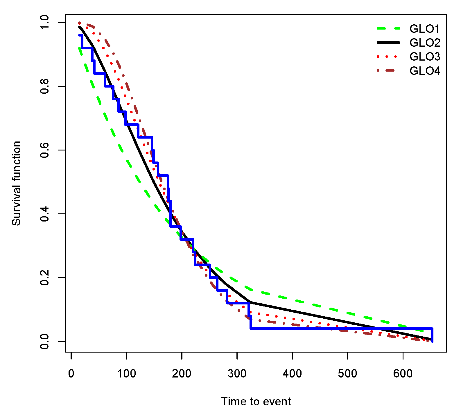
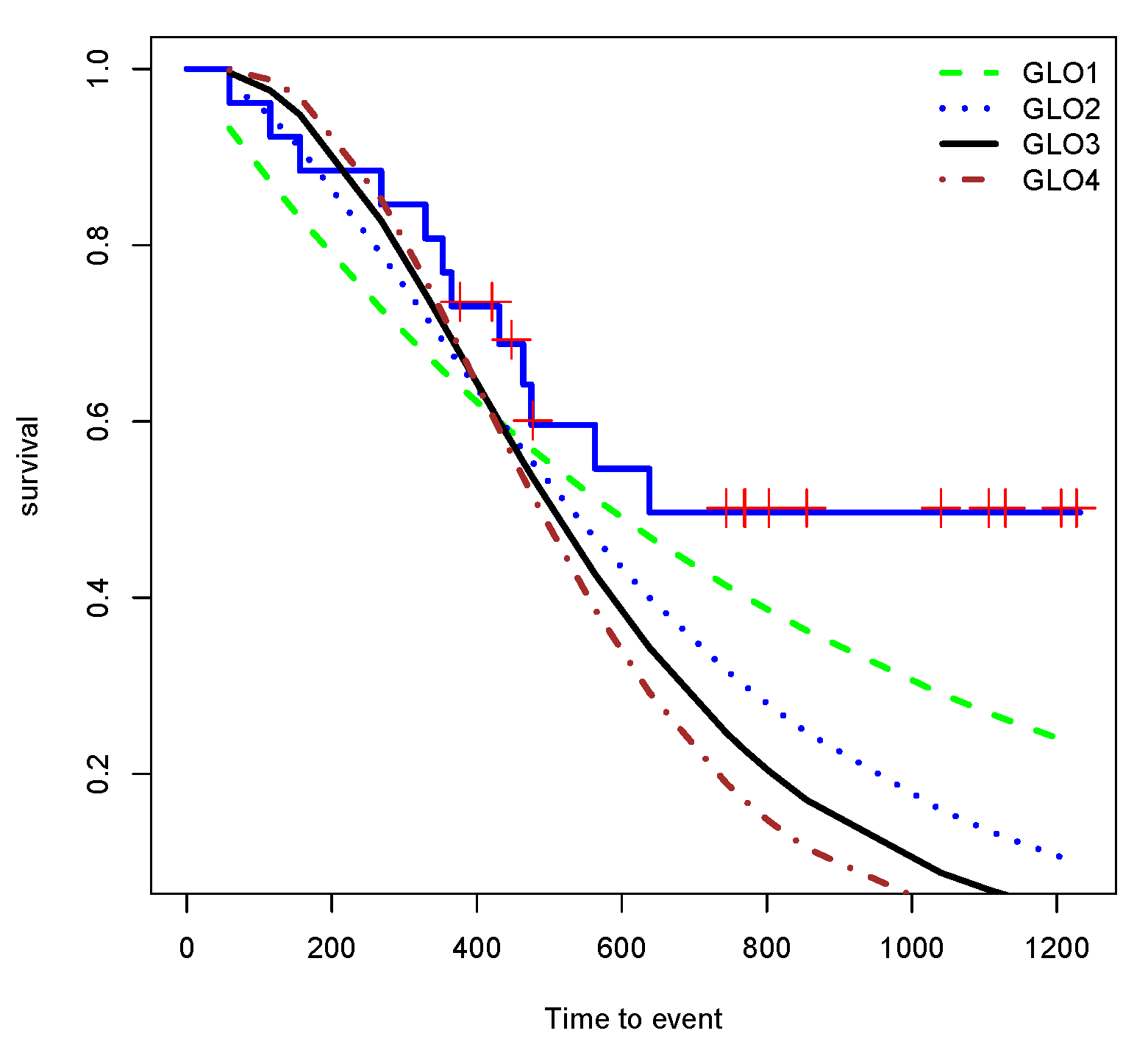
Edmunson et al. [30] considered survival data related to some ovarian cancer patients. The data set has also been reported in ‘survival’ package in R and includes variables ‘futime’ indicating time to death or censoring of the patients and ‘fustat’ as censoring status. Table 7 shows results of fitting data to GLOm for and 4. Based on the log-likelihood measure, among these models, GLO3 describe the data better. The Kaplan-Meier survival function along with GLOms have been drawn in Figure 5.
6. Conclusions
Lindley distribution which is a mixture of gamma models has attracted the attention of many researchers in recent decades. It has been shown that this distribution is quite useful in describing real data sets. Over and above that, extensions of this model have also been introduced in the literature. Here, we introduced a fresh method to generalize the Lindley distribution which the flexibility rises by increasing the number of mixed components in the model. The proposed model is called the GLOm where m represents the number of baseline models called the order of the model. We studied some properties of GLOm for different m. The moments, the variance and the moment generating function were shown to have closed forms for every m. The MLE of the parameter have been discussed for either of the right censored data and the complete data. The supplied simulation results indicated that the MLE is suitable for both the censored data and the non-censored data. Two real data sets were discussed showing that generalizing the Lindley distribution as accomplished in this paper may be helpful to describe the data more conveniently.
Author Contributions
Formal analysis, A.A. and M.K.; Investigation, M.K.; Methodology, A.A. and M.K.; Software, A.A.; Writing—original draft, A.A. All authors have read and agreed to the published version of the manuscript.
Funding
This Project was funded by the National Plan for Science, Technology and Innovation (MAARIFAH), King Abdulaziz City for Science and Technology, Kingdom of Saudi Arabia, Award Number (14-MAT2052-02).
Acknowledgments
The authors are grateful to anonymous referees for their constructive comments that lead to an improvement in the quality of the paper. The authors would like to extend their sincere appreciation to the strategic technology program of the National Plan for Science, Technology and Innovation in the Kingdom of Saudi Arabia for its funding this project No. 14-MAT2052-02.
Conflicts of Interest
There is not conflict of interest.
References
- Lindley, D.V. Fiducial distributions and Bayes’ theorem. J. R. Stat. Soc. Ser. (Methodol.) 1958, 20, 102–107. [Google Scholar] [CrossRef]
- Cakmakyapan, S.; Ozel, G. The Lindley family of distributions: Properties and applications. Hacet. J. Math. Stat. 2017, 46, 1113–1137. [Google Scholar] [CrossRef]
- Ghitany, M.E.; Atieh, B.; Nadarajah, S. Lindley distribution and its application. Math. Comput. Simul. 2008, 78, 493–506. [Google Scholar] [CrossRef]
- Sankaran, M. The discrete poisson-Lindley distribution. Biometrics 1970, 26, 145–149. [Google Scholar] [CrossRef]
- Ghitany, M.E.; Al-Mutairi, D.K.; Nadarajah, S. Zero-truncated Poisson-Lindley distribution and its application. Math. Comput. Simul. 2008, 79, 279–287. [Google Scholar] [CrossRef]
- Zamani, H.; Ismail, N. Negative Binomial-Lindley Distribution and Its Application. J. Math. Stat. 2010, 6, 4–9. [Google Scholar] [CrossRef] [Green Version]
- Ghitany, M.E.; Al-Mutairi, D.K.; Awadhi, F.A.; Alburais, M. Marshall-Olkin extended Lindley distribution and its application. Int. J. Appl. Math. 2012, 25, 709–721. [Google Scholar]
- Ghitany, M.E.; Al-Mutairi, D.K.; Balakrishnan, N.; Al-Enezi, L.J. Power Lindley distribution and associated inference. Comput. Stat. Data Anal. 2013, 64, 20–33. [Google Scholar] [CrossRef]
- Al-Mutairi, D.K.; Ghitany, M.E.; Kundu, D. Inferences on stress-strength reliability from Lindley distribution. Commun. Stat.-Theory Methods 2013, 42, 1443–1463. [Google Scholar] [CrossRef]
- Al-babtain, A.A.; Eid, H.A.; A-Hadi, N.A.; Merovci, F. The five parameter Lindley distribution. Pak. J. Stat. 2014, 31, 363–384. [Google Scholar]
- Ghitany, M.E.; Al-Mutairi, D.K.; Aboukhamseen, S.M. Estimation of the reliability of a stress-strength system from power Lindley distributions. Commun. Stat.-Simul. Comput. 2015, 44, 118–136. [Google Scholar] [CrossRef]
- Al-Mutairi, D.K.; Ghitany, M.E.; Kundu, D. Inferences on stress-strength reliability from weighted lindley distributions. Commun. Stat.-Theory Methods 2015, 44, 4096–4113. [Google Scholar] [CrossRef]
- Abouammoh, A.M.; Alshangiti Arwa, M.; Ragab, I.E. A new generalized Lindley distribution. J. Stat. Comput. Simul. 2015, 85, 3662–3678. [Google Scholar] [CrossRef]
- Shanker, R.; Fesshaye, H.; Sharma, S. On Two-Parameter Lindley Distribution and its Applications to Model Lifetime Data. Biom. Biostat. Int. J. 2016, 1, 9–15. [Google Scholar] [CrossRef]
- Shanker, R.; Mishra, A. A quasi Lindley distribution. Afr. J. Math. Comput. Sci. Res. 2013, 6, 64–71. [Google Scholar]
- Shanker, R.; Ghebretsadik, A.H. A New Quasi Lindley Distribution. Int. J. Stat. Syst. 2013, 8, 143–156. [Google Scholar]
- Merovci, F.; Sharma, V.K. The Beta-Lindley Distribution: Properties and Applications. J. Appl. Math. 2014, 2014, 198951. [Google Scholar] [CrossRef]
- Zakerzadeh, H.; Dolati, A. Generalized Lindley distribution. J. Math. Ext. 2009, 3, 13–25. [Google Scholar]
- Ibrahim, E.; Merovci, F.; Elgarhy, M. A new generalized Lindley distribution. Math. Theory Model. 2013, 3, 30–47. [Google Scholar]
- Shanker, R.; Shukla, K.K.; Shanker, R.; Leonida, T.A. A Three-Parameter Lindley Distribution. Am. J. Math. Stat. 2017, 7, 15–26. [Google Scholar]
- Broderick, O.O.; Tiantian, Y. A new class of generalized Lindley distributions with applications. J. Stat. Comput. Simul. 2015, 85, 2072–2100. [Google Scholar] [CrossRef]
- Wolstenholme, L.C. Reliability Modelling: A Statistical Approach; Chapman and Hall/CRC: London, UK, 1999; ISBN 9781584880141. [Google Scholar]
- McPherson, J.W. Reliability Physics and Engineering: Time-To-Failure Modeling; Springer: Berlin/Heidelberg, Germany, 2010; ISBN 978-1-4419-6348-2. [Google Scholar]
- Cheng, R.; Feast, G. Some Simple Gamma Variate Generators. J. R. Stat. Soc. Ser. C (Appl. Stat.) 1979, 28, 290–295. [Google Scholar] [CrossRef]
- Bulmer, M.G. Principles of Statistics; Dover: New York, NY, USA, 1979; ISBN 0-486-63760-3. [Google Scholar]
- Lai, C.D.; Xie, M. Stochastic Aging and Dependence for Reliability; Springer: New York, NY, USA, 2006; ISBN 978-0-387-29742-2. [Google Scholar]
- Shao, J. Mathematical Statistics; Springer: New York, NY, USA, 2003. [Google Scholar] [CrossRef]
- Fleming, T.R.; Harrington, D.P. Counting Processes and Survival Analysis; Wiley: Hoboken, NJ, USA, 2011; ISBN 978-1-118-15066-5. [Google Scholar]
- Lawless, J.F. Statistical Models and Methods for Lifetime Data, 2nd ed.; Wiley: Hoboken, NJ, USA, 2003. [Google Scholar]
- Edmunson, J.H.; Fleming, T.R.; Decker, D.G.; Malkasian, G.D.; Jefferies, J.A.; Webb, M.J.; Kvols, L.K. Different Chemotherapeutic Sensitivities and Host Factors Affecting Prognosis in Advanced Ovarian Carcinoma vs. Minimal Residual Disease. Cancer Treat. Rep. 1979, 63, 241–247. [Google Scholar]
Publisher’s Note: MDPI stays neutral with regard to jurisdictional claims in published maps and institutional affiliations. |
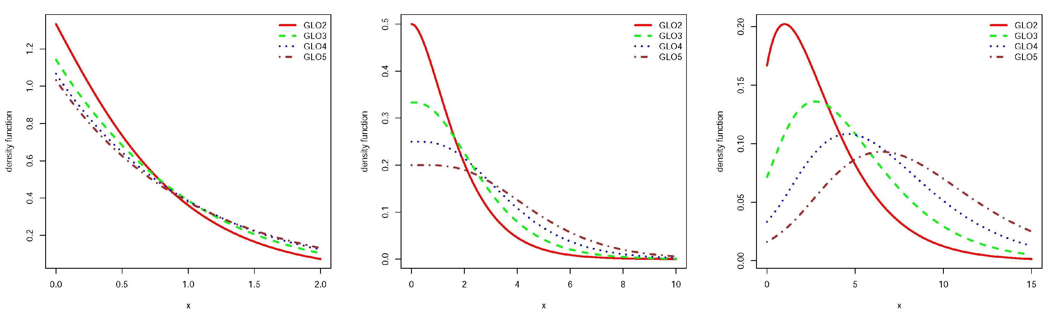
Figure 1.
Density function for GLO2, GLO3, GLO4 and GLO5 and and from left to right respectively.

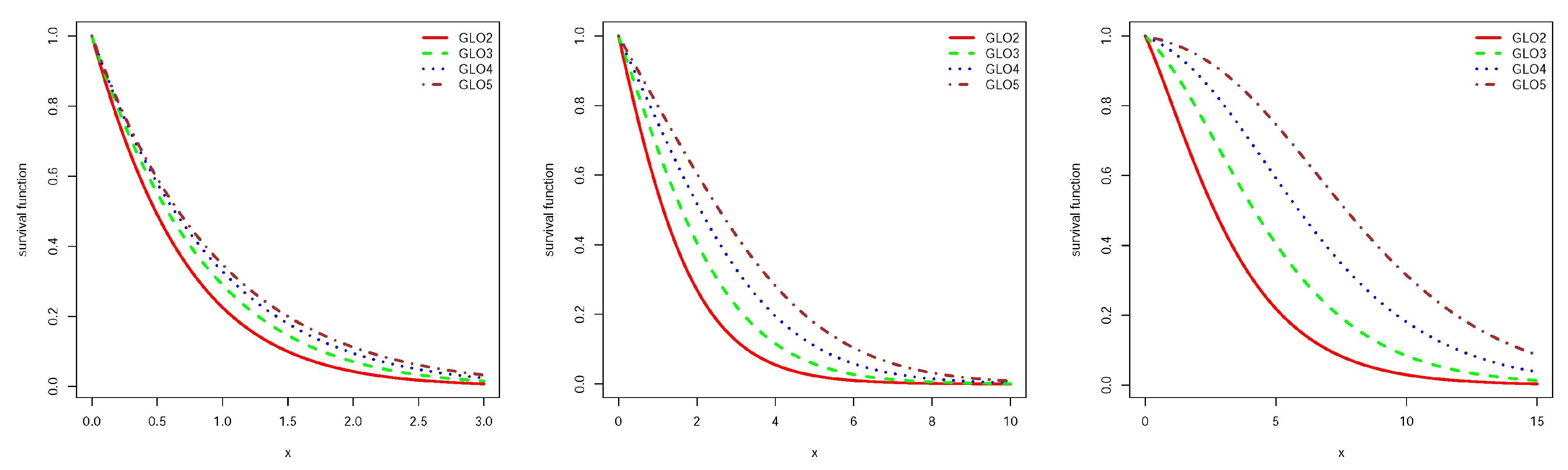
Figure 2.
Survival function for GLO2, GLO3, GLO4 and GLO5 and and from left to right respectively.

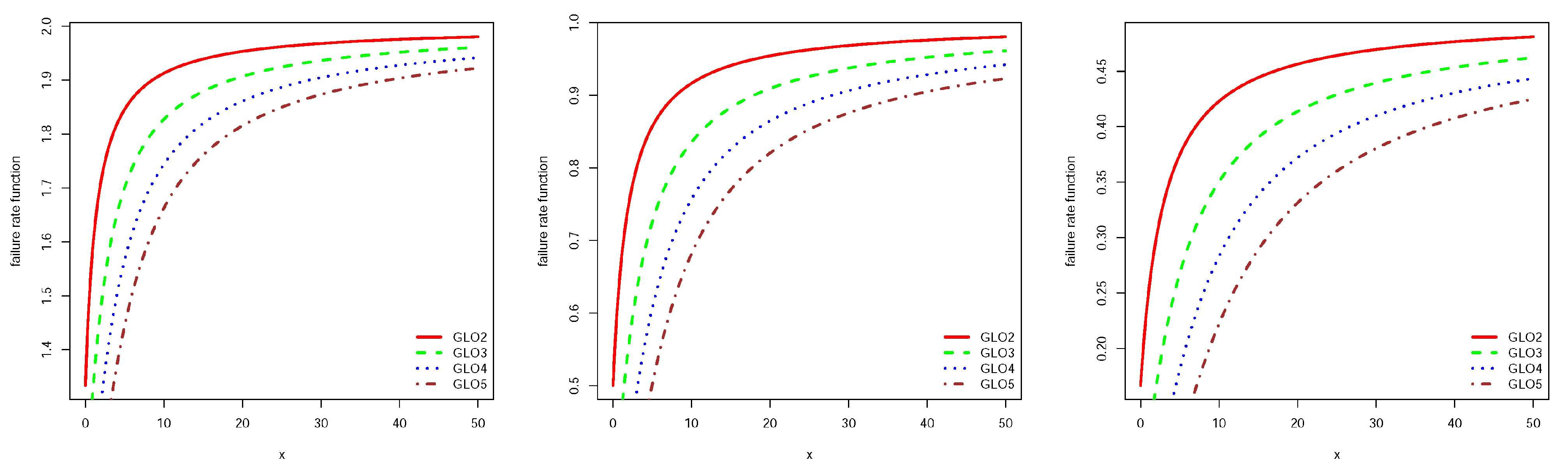
Figure 3.
Failure rate function for GLO2, GLO3, GLO4 and GLO5 and and from left to right respectively.
Figure 3.
Failure rate function for GLO2, GLO3, GLO4 and GLO5 and and from left to right respectively.

Figure 4.
Empirical survival function and survival function of fitted GLOm.

Figure 5.
Kaplan-Meier survival function and survival function of fitted GLOm.


Table 1.
PDF, CDF, mean and failure rate for generalized Lindley random variables of orders 2, 3 and 4.
Table 1.
PDF, CDF, mean and failure rate for generalized Lindley random variables of orders 2, 3 and 4.
| GLO2 | GLO3 | GLO4 | |
|---|---|---|---|
| CDF | |||
| Mean | |||
| Failure rate |
Table 2.
Simulation results for estimating .
| m | B | |||
|---|---|---|---|---|
| 2 | 0.01 | 0.000392 | 0.001285 | 0.000002 |
| 0.2 | 0.003687 | 0.027083 | 0.001223 | |
| 2 | 0.089519 | 0.303592 | 0.156634 | |
| 3 | 0.01 | 0.000212 | 0.001064 | 0.000001 |
| 0.2 | 0.003756 | 0.021395 | 0.000725 | |
| 2 | 0.065359 | 0.260616 | 0.113436 | |
| 4 | 0.01 | 0.000223 | 0.000956 | 0.000001 |
| 0.2 | 0.002531 | 0.018226 | 0.000538 | |
| 2 | 0.067082 | 0.234948 | 0.090523 | |
| 5 | 0.01 | 0.000036 | 0.000827 | 0.000001 |
| 0.2 | 0.001806 | 0.016431 | 0.000420 | |
| 2 | 0.048145 | 0.205068 | 0.072493 | |
| 6 | 0.01 | 0.000089 | 0.000762 | 0.000000 |
| 0.2 | 0.000261 | 0.014639 | 0.000346 | |
| 2 | 0.048055 | 0.203754 | 0.068692 |
Table 3.
Simulation results for estimating when 25% of the sample has been censored from right.
| n | m | B | |||
|---|---|---|---|---|---|
| 20 | 2 | 0.01 | 0.000228 | 0.001437 | 0.000003 |
| 0.2 | 0.005887 | 0.029532 | 0.001384 | ||
| 1.2 | −0.218137 | 0.218137 | 0.055005 | ||
| 3 | 0.01 | 0.000192 | 0.001251 | 0.000002 | |
| 0.2 | 0.001745 | 0.022546 | 0.000809 | ||
| 1.2 | −0.209398 | 0.209398 | 0.044895 | ||
| 4 | 0.01 | 0.000066 | 0.000936 | 0.000001 | |
| 0.2 | 0.002496 | 0.019698 | 0.000614 | ||
| 1.2 | −0.204693 | 0.204693 | 0.042309 | ||
| 5 | 0.01 | 0.000041 | 0.000888 | 0.000001 | |
| 0.2 | 0.001541 | 0.018230 | 0.000541 | ||
| 1.2 | −0.202124 | 0.202124 | 0.040991 | ||
| 40 | 2 | 0.01 | 0.000041 | 0.001018 | 0.000001 |
| 0.2 | 0.002479 | 0.020986 | 0.000699 | ||
| 1.2 | −0.206282 | 0.206282 | 0.043137 | ||
| 3 | 0.01 | 0.000012 | 0.000769 | 0.000001 | |
| 0.2 | 0.001470 | 0.015627 | 0.000389 | ||
| 1.2 | −0.202902 | 0.202902 | 0.041378 | ||
| 4 | 0.01 | 0.000029 | 0.000694 | 0.000000 | |
| 0.2 | 0.001004 | 0.014321 | 0.000313 | ||
| 1.2 | −0.201060 | 0.201060 | 0.040472 | ||
| 5 | 0.01 | 0.000002 | 0.000636 | 0.000000 | |
| 0.2 | −0.000065 | 0.012032 | 0.000226 | ||
| 1.2 | −0.200265 | 0.200265 | 0.040113 |
Table 4.
Simulation results for estimating when 40% of the sample has been censored from right.
| n | m | B | |||
|---|---|---|---|---|---|
| 20 | 2 | 0.01 | 0.000307 | 0.001546 | 0.000003 |
| 0.2 | 0.003416 | 0.032657 | 0.001677 | ||
| 1.2 | −0.221936 | 0.221936 | 0.053017 | ||
| 3 | 0.01 | 0.000057 | 0.001298 | 0.000002 | |
| 0.2 | 0.000150 | 0.024646 | 0.000981 | ||
| 1.2 | −0.216420 | 0.216420 | 0.049195 | ||
| 4 | 0.01 | −0.000017 | 0.001050 | 0.000002 | |
| 0.2 | 0.001599 | 0.021568 | 0.000731 | ||
| 1.2 | −0.206033 | 0.206033 | 0.043004 | ||
| 5 | 0.01 | −0.000027 | 0.000901 | 0.000001 | |
| 0.2 | 0.001679 | 0.018990 | 0.000585 | ||
| 1.2 | −0.203726 | 0.203726 | 0.041973 | ||
| 40 | 2 | 0.01 | 0.000093 | 0.001088 | 0.000002 |
| 0.2 | 0.000000 | 0.021989 | 0.000781 | ||
| 1.2 | −0.211623 | 0.211623 | 0.046143 | ||
| 3 | 0.01 | 0.000072 | 0.000867 | 0.000001 | |
| 0.2 | −0.000216 | 0.016417 | 0.000432 | ||
| 1.2 | −0.205086 | 0.205086 | 0.042572 | ||
| 4 | 0.01 | −0.000024 | 0.000739 | 0.000000 | |
| 0.2 | 0.000730 | 0.014284 | 0.000318 | ||
| 1.2 | −0.202220 | 0.202220 | 0.041028 | ||
| 5 | 0.01 | 0.000014 | 0.000652 | 0.000000 | |
| 0.2 | −0.000495 | 0.012862 | 0.000261 | ||
| 1.2 | −0.201258 | 0.201258 | 0.040596 |
Table 5.
Number of cycles to failure for 25 specimens yarn.
| 15 | 20 | 38 | 42 | 61 | 76 | 86 | 98 | 121 | 146 | 149 | 157 | 175 |
| 176 | 180 | 180 | 198 | 220 | 224 | 251 | 264 | 282 | 321 | 325 | 653 |
Table 6.
Estimate of and -log-likelihood for GLOm with different m values.
| m | -log-likelihood | ||
|---|---|---|---|
| 1 | 0.00560 | 0.00000125 | 154.5895 |
| 2 | 0.01116 | 0.00000249 | 152.5070 |
| 3 | 0.01674 | 0.00000373 | 154.5319 |
| 4 | 0.02230 | 0.00000497 | 158.1863 |
Table 7.
Estimate of and -log-likelihood for GLOm with different m values.
| m | -log-likelihood | ||
|---|---|---|---|
| 1 | 0.00118 | 0.00000019 | 92.8365 |
| 2 | 0.00316 | 0.00000028 | 90.0980 |
| 3 | 0.00529 | 0.00000057 | 89.7396 |
| 4 | 0.00752 | 0.00000085 | 90.2579 |
© 2020 by the authors. Licensee MDPI, Basel, Switzerland. This article is an open access article distributed under the terms and conditions of the Creative Commons Attribution (CC BY) license (http://creativecommons.org/licenses/by/4.0/).
Share and Cite
MDPI and ACS Style
Abouammoh, A.; Kayid, M. A New Flexible Generalized Lindley Model: Properties, Estimation and Applications. Symmetry 2020, 12, 1678. https://doi.org/10.3390/sym12101678
AMA Style
Abouammoh A, Kayid M. A New Flexible Generalized Lindley Model: Properties, Estimation and Applications. Symmetry. 2020; 12(10):1678. https://doi.org/10.3390/sym12101678
Chicago/Turabian StyleAbouammoh, Abdulrahman, and Mohamed Kayid. 2020. "A New Flexible Generalized Lindley Model: Properties, Estimation and Applications" Symmetry 12, no. 10: 1678. https://doi.org/10.3390/sym12101678
Note that from the first issue of 2016, this journal uses article numbers instead of page numbers. See further details here.