Relativistic Effects in Orbital Motion of the S-Stars at the Galactic Center


1
SPb Branch of Special Astrophysical Observatory of Russian Academy of Sciences, 65 Pulkovskoye Shosse, 196140 St. Petersburg, Russia
2
Astrophysics Department, Mathematics & Mechanics Faculty, Saint Petersburg State University, 28 Universitetskiy Prospekt, 198504 St. Petersburg, Russia
*
Authors to whom correspondence should be addressed.
Universe 2020, 6(10), 177; https://doi.org/10.3390/universe6100177
Submission received: 19 September 2020
/
Revised: 6 October 2020
/
Accepted: 8 October 2020
/
Published: 14 October 2020
(This article belongs to the Special Issue Selected Papers from the 17th Russian Gravitational Conference —International Conference on Gravitation, Cosmology and Astrophysics (RUSGRAV-17))
Abstract
:The Galactic Center star cluster, known as S-stars, is a perfect source of relativistic phenomena observations. The stars are located in the strong field of relativistic compact object Sgr A* and are moving with very high velocities at pericenters of their orbits. In this work we consider motion of several S-stars by using the Parameterized Post-Newtonian (PPN) formalism of General Relativity (GR) and Post-Newtonian (PN) equations of motion of the Feynman’s quantum-field gravity theory, where the positive energy density of the gravity field can be measured via the relativistic pericenter shift. The PPN parameters and are constrained using the S-stars data. The positive value of the component of the gravity energy–momentum tensor is confirmed for condition of S-stars motion.
1. Introduction
The S-stars cluster in the Galactic Center [1,2,3,4] is a unique observable object to investigate. Once for the orbital period, the stars pass their pericenters, where they reach high velocities (∼0.01 or even ∼0.1 of the speed of light for the most recent discovered stars [5]) and get close to the relativistic compact object Sgr A*. Such conditions lead to manifestation of relativistic effects in proximity to a supermassive compact object (Super-Massive Black Hole). Therefore, we are able to explore them in the frame of Post-Newtonian formalism. For recent overviews of General Relativity (GR) see, e.g., Debono and Smoot [6] and references therein.
The Post-Newtonian formalism is a tool which provides an opportunity to express the relativistic equations of gravity as the small-order deviations from the Newtonian theory. The Parameterized Post-Newtonian formalism can be implemented to various theories of gravity [7]. It is a version of the PN formalism that has a parameters that quantitatively express the difference of a theory of gravity and the Newtonian theory. In this work, the parameters of and , which appear in the expansion of the Schwarzschild solution [8], are taken into consideration. Even in the solar system, physical effects can be detectable via the PPN formalism. The most precise constrain of the parameter (with the accuracy of ) was obtained using the data from the Cassini experiment [9]. The detected effect was the the time delay, which is also known as the classical fourth test of general relativity by Shapiro [10]. The PPN parameters and were also measured with the EPM2017 ephemerides [11,12]. It turns out that is at the level as well, and that also the measurement is reaching the Cassini experiment level. In particular, [13] delivers and [14] yields . Iorio [11], relying upon recent EPM data, suggests a level. In the modern solar system experiments, even the second-order PN effects are being investigated [15,16]. The PPN formalism is a promising approach in testing cosmological models [17].
Post-Newtonian equations of motion also can be used for a possible solution of the well-known problem of pseudo-tensor of the energy–momentum tensor of the gravitational field in GR (Landau and Lifshitz [18] (Par. 101 “The energy-momentum pseudotensor”, p. 304) and review Baryshev [19]). The point is that in the frame of the Feynman’s relativistic quantum-field approach to gravitational interaction [20] there is ordinary (not “pseudo”) energy–momentum tensor of the gravity field. So there is positive localizable energy density of the gravitational field , which in the case of the PN approximation equals . Fortunately, this energy–mass distribution around central massive body gives 16.7% contribution to the relativistic pericenter shift and together with linear part gives the standard value of the Mercury perihelion shift [21].
The S-stars were being used in a big amount of different investigations. The most interesting in the context of this work are investigations of the motion of the S-stars. The possibility of detecting the Post-Newtonian effects in the motion of S2 was being researched some time ago [22]. It was shown that the perturbations produced by these effects are significant and have a specific time dependence. In the work Parsa et al. [23], the authors used the PN approximation to calculate the stellar orbits and investigate how do they change if the fitting is employed in different parts of the orbit. The important effects that can be seen in the S-stars data are the effects related to the light propagation. It is possible to investigate the relativistic redshift using the spectroscopic data. The authors of work Saida et al. [24] show that there is a double-peak-appearance in the time evolution of the defined GR evidence.
The purpose of this work is to consider the relativistic Post-Newtonian motion of several S-stars, using the data from the work [25], and to attract attention to the theoretical uncertainty in analysis of PN motion of S-stars due to coordinate dependence of the orbital shapes of the PN test body motion in GR. Additionally in the frame of the Feynman’s field-theoretical approach (FGT) we estimate the energy density of the static gravitational field for S-stars conditions.
The effects related to spin of the central massive object, such as Lense–Thirring precession, are also detectable via observations of the most recently discovered S-stars [5,26,27]. It is important that we consider only the Schwarzschild problem and do not take the spin-related effects into consideration, which we shall study in separate paper.
2. Observational Data
The S-stars cluster has been observed for 25 years now. This period of time is comparable with the orbital periods of the stars. Some of them have made a revolution of their orbit, and in particular cases it is even not a single time. The accumulated arrays of data differ in their meaningfullness for different S-stars. The star named S2 is the most popular choice among the researchers, and it is not unreasonable. The S2 is the most thoroughly observed, so it has the biggest time series of the observational data. We will consider this star, along with the stars S38 and S55.
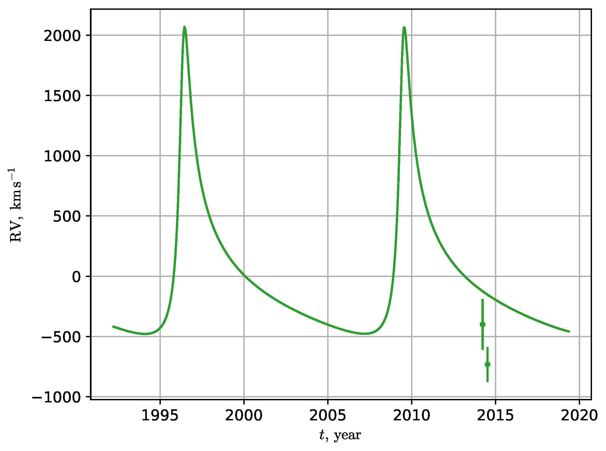
There are two types of S-stars observational data: the astrometric and the spectroscopic one. The astrometric data are given as the visual positions of the S-stars on the sky. It is important that one should take into account not only the pair of coordinates, but also the time of the observations. At first sight, it may seem to the reader that to obtain the best-fit trajectory, one should implement the fitting procedures that use the points of visual positions of the stars to fit the ellipses into them as the visual trajectories. What these procedures actually fit are not 2D ellipses, but spirals in the 3D space with the axes of not only right ascension and declination, but also the time of the observed positions. The spectroscopic data consist of radial velocities, corrected with respect to the Local Standard of the Rest (the so-called VLSR correction) of the S-stars. We cannot use the modeled velocities directly to fit the observed radial velocities. We shall interpret the latter as the redshift values. The modeled radial velocities must be transformed to observable values with the Equation (9) so the relativistic Doppler effect and the gravitational redshift are taken into account.
The dataset that we use is described in previous work [25]. It is a dataset combined from the data of 4 works Gillessen et al. [4], Boehle et al. [28], Chu et al. [29], and Do et al. [30]. It contains the astrometric and the spectroscopic data of S2, S38, and S55 obtained on VLT, Keck observatory, and Subaru telescope. The data presented in different works must be corrected for difference in the reference system [4,31].
3. Post-Newtonian Effects
3.1. Equations of Motion
For the purpose of this work, it is important to use the equations of motion, which will be integrated to simulate the S-stars trajectories. In the frame of geometrical General Relativity theory (GR), according to classical textbook by Brumberg [32] (1991), the Post-Newtonian equations of motion of a test particle in the static gravitational field of central massive body are given by
where denotes the coordinate system choice. For example, for the Standard (Schwarzschild) coordinates and for either isotropic or harmonic coordinates the parameter . Note that, though the secular effects do not depend on the parameter , the shape of the orbit is different for different . For the purposes of the relativistic celestial mechanics, the isotropic coordinate system is more commonly used, as it is stated in Misner et al. [8]. Here, it is important to note that modern S-stars observations allow, for the first time, to measure directly the shape of the S-star orbit, which means to test the value of the parameter itself. This raises a question about the role of the coordinate system choice in GR.
For isotropic or harmonic coordinates, the parameter , so the corresponding PN equations of motion in the frame of GR are
Intriguingly, these equations of motion coincide with the PN equations of motion in the Feynman’s field-theoretical approach to gravitation (FGT) ([21,33]), where they do not depend on the choice of coordinate system. Importantly, the term includes the non-linear part: factor , where 3 is the linear part and 1 is the non-linear part. This non-linear part corresponds to the contribution of the effective radial mass–energy density distribution of the gravitational field itself around the central body
This additional mass distribution gives correction to the 00-component of the tensor gravitational potential in the form:
which leads to the non-linear part of the relativistic pericenter shift. Derivations of all needed equations and possible applications of the PN equations of motion are presented in review [19].
The PPN generalization of the Schwarzschild metric in the frame of isotropic coordinates leads to the PPN equations of motion [25], which are given by
Substituting leads to GR PN equations in the frame of the isotropic or harmonic coordinate systems. We can see that in the limit these equations reduce to Newtonian equations of motion
In the work of Brumberg [32], the author considered the problem in a more general way. He did also obtain PPN equations of motion, but the coordinate system that he considered was not fixed. This fact implies that there appears the corresponding third degree of freedom, which is related to the coordinate system choice. Therefore, Brumberg [32] used to have 3 PPN parameters , instead of the 2 usual PPN parameters .
3.2. Pericenter Shift
The Post-Newtonian equations of motion lead us into the effect of the pericenter shift. The value of the pericenter shift per one turn in GR is well known [32,34]
where a is a semi-major axis, e is an eccentricity, and is a gravitational radius.
From coincidence of the PN equations of a test particle motion in GR and FGT, it follows that the expression for the pericenter shift in FGT and GR is exactly the same. The difference from GR is that the FGT formula has two different terms:
The first term with a factor of corresponds to the linear approximation, when in the field equations one does not take into account the non-linear contribution (energy of gravitational field itself). The second term with a factor of occurs after taking into account the non-linearity due to the positive energy density of the gravitational field. This term corresponds to the measurement of the field energy of the gravitation via pericenter shift observations.
The pericenter shift values and parameter of in pericenter predicted for S-stars are presented in the Table 1.
The observable effect is similar to one with the Mercury anomalous pericenter shift, that Einstein explained. The effect of GR Schwarzschild perihelion precession was also measured with artificial Earth satellites [35,36], so this effect is well studied in the solar system. Now we can observe it with S-star cluster in the center of our Galaxy. For Mercury, the pericentral is , and for binary pulsar PSR 1913 + 16 it is . We can see that the field at the pericenter of the S-stars orbits is stronger by 2 orders of magnitude.
Although the values of the pericenter shift seem to be small, they are actually detectable, which is shown in the recent work of GRAVITY collaboration [31]. The pericenter shift appears as a consequence of the PN equations of motion. That means that using the PN equations of motion to fit the trajectories implies detecting the pericenter shift effect. In the frame of field approach, it means that we are able to measure the field energy density, which is positive and localizable.
3.3. Light Propagation
We must take into consideration several relativistic effects related to light propagation. Such as the relativistic Doppler effect, which is the reason we must transform modeled RVs to the observable RVs. Another significant light propagation effect is the gravitational redshift, which was successfully measured by Do et al. [30]. Taking both of these effects into account is described in [25] by the equation
The detailed study of this effect is described in the work of Iorio [37].
It is also necessary to take into account the Rømer delay. The gravitational lensing and Shapiro time delay effects are negligible in this problem.
4. Modeling
4.1. Parameters
Our aim was to build a model of the S-stars observations which depends on PPN parameters and . After that, we will be able to use some of the optimization techniques to solve the inverse problem and estimate the parameters. The question is how many parameters do we need to build a model.
To define the orbit and the position of the star, we need 6 parameters. For example, these could be Keplerian parameters or the components of the initial phase vector. The coordinate system that we use is defined as follows: the plane is the sky itself, where y axis points in the direction of declination, x axis has the reversed direction of right ascension, and the z axis is pointed from Sgr A* to the observer. The next 2 parameters that we need are the mass of Sgr A* and the distance to the Galactic Center. The Sgr A* itself also has the velocity relative to our solar system, so we have two more parameters of its initial position on the sky (which alongside with the distance form the vector of the Sgr A* position relative to the solar system.) and 3 parameters, which define its velocity. The dataset that we use contains 3 different observational data arrays, that were obtained by different teams, and hence have their own different reference frames. The biggest observational dataset is the one from Gillessen et al. [4]. We will use it as the reference observational dataset aligned with our coordinate system. As we have two more datasets (from the papers [28,30]), we must add 4 more parameters, which are the RA and Dec offsets from the dataset of [28] or [30] and the reference dataset of [4]. The final 2 of our parameters are the PPN parameters of and that we want to constrain. In total, we have 19 parameters if we consider 1 star, or 31 parameters if we consider 3 stars. It is a large amount of parameters. In the next section, it is shown that the model construction implies very non-trivial dependency of the likelihood function from the parameters. As a result of this, along with the large amount of parameters, we decided to use the Bayesian inference techniques, such as the MCMC sampling.
4.2. Constructing a Model
The first step in the modeling is to find the trajectory. We want to integrate the equations of motion in a 2D plane. For this purpose, we need 4 parameters of initial phase vector components . They are used as the initial conditions for the integrator, which is the Owren–Zennano 4/3-order method implemented in the DifferentialEquations package [38] of the Julia language [39]. It produces the array of phase vectors , which is a modeled trajectory. To rotate it, we need 2 angles: the longitude of the ascending node and the inclination i, which are the remaining 2 parameters. To perform the rotations, one should pad the modeled array of phase vectors to 6D phase space , where z and are zeros. After that, one should multiply each triplet of coordinates and velocities with the rotation matrices that contain and i. As the result, one will obtain the modeled array of phase vectors in the reference frame that is needed. In total, we have 6 parameters that define the orbit and the position of the star, as it was stated before.
The next step is getting RA and Dec from x and y of modeled trajectory. The Rømer time delay is taken into account at this step. We shall divide the coordinates by , but one important thing is the sign. We should inverse x, as the RA scale is clockwise. We also must take into account the proper motion of Sgr A*.
Finally, we have to obtain RV from , using the Equation (9) due to the light propagation effects.
5. MCMC Analysis
Bayesian inference is the statistical method of inference in which the probability of a hypothesis is updated with the Bayes’s theorem
where H stands for the hypothesis and E stands for evidence. The is a likelihood. It is a probability of observing the data (evidence) given hypothesis. is called model evidence or the marginalized likelihood. stands for the prior probability (the probability of hypothesis before taking the observed data into the account) and is the posterior probability (after taking the data into account). In the context of the Bayesian parameter inference, the Bayes’s theorem may be interpreted as
where is a sample of the observed data and is a vector of the parameters. is a prior distribution of the parameters, is the likelihood, and is a posterior distribution of the parameters.
Once the model is defined, it is possible to simulate the data values and compare them with the real observable values. To do that, one can define the chi-squared residuals and the likelihood function. The latter can be used by the Markov Chain Monte Carlo sampler. We use the one implemented in the AffineInvariantMCMC package (documentation available at https://github.com/madsjulia/AffineInvariantMCMC.jl) for The Julia language [39]. Using the MCMC sampling, one can obtain the constraints of parameters of a defined model.
In the previous work [25], some of the parameters were considered to be fixed, so the model was simplified and had a lesser amount of the parameters. However, in the work [31], it is stated that this simplification leads to the uncertainties. In our case, this is taken into account and the model now depends on 31 parameters. The process was launched with 300 independently computed chains (the so-called ‘walkers’), where each chain consists of the parameters and corresponding log-likelihood values for 2000 iterations.
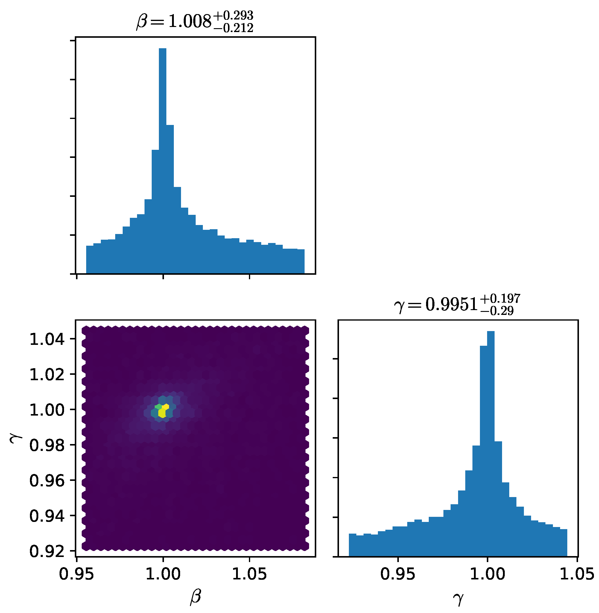
The posterior distributions of the and are presented in Figure 1. The right and top plots show us the histograms of the posterior distributions of the considered parameters. The bottom-left plot is a ‘2D-histogram’ of these parameters, where the color shows us the amount of points in a bin. This ‘2D-histogram’ is actually a projection of our 31-dimensional posterior distribution of the parameters to the 2D plane of and parameters. We can see that the PPN parameters do not make a significant contribution to the model. Therefore, these parameters have relatively high errors. It is possible to constrain the PPN parameters with this approach. The errors are much smaller than in the previous work [25].
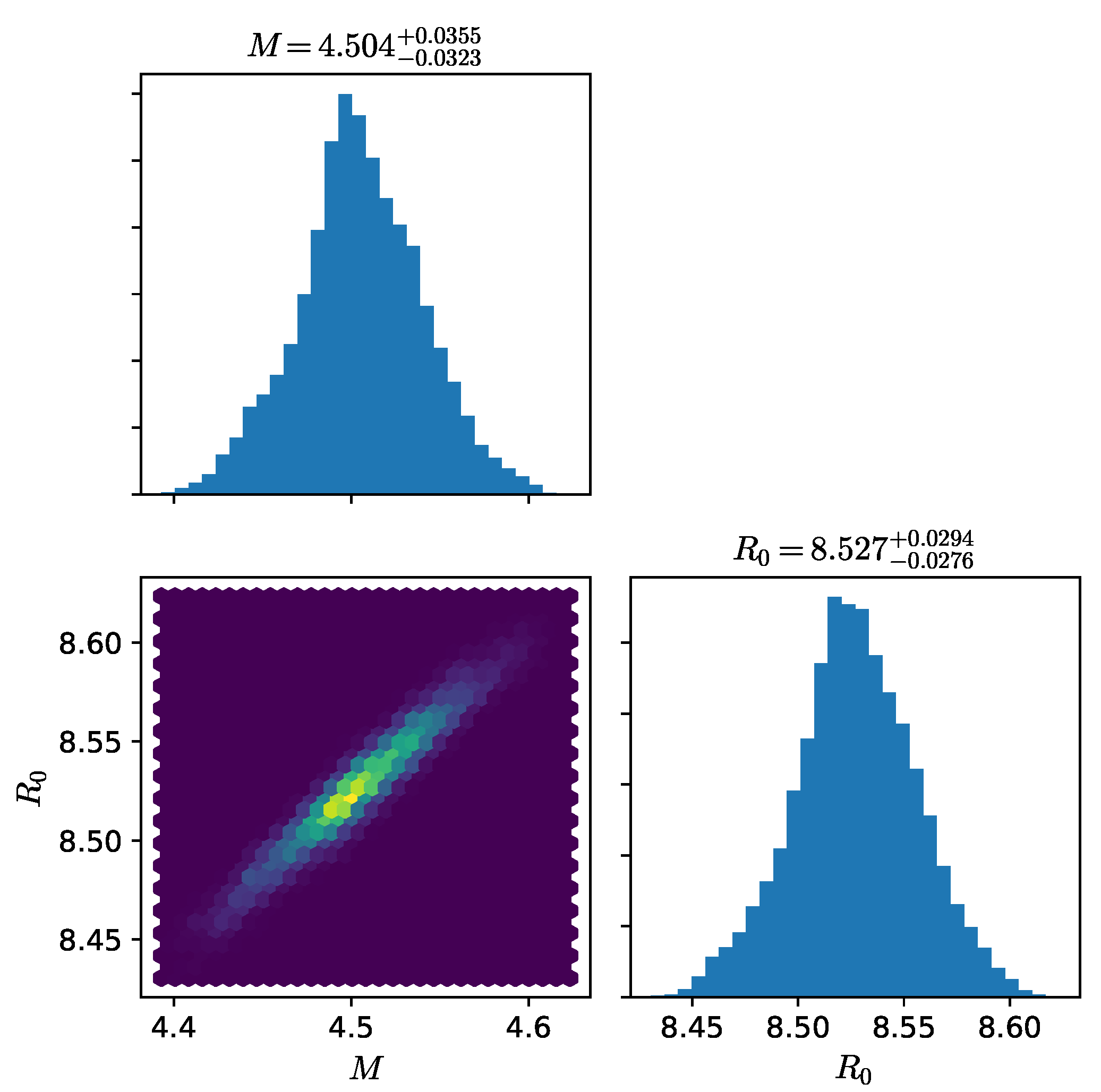
The other important parameters constrained by our model are the mass of Sgr A* in the units of and the distance to the Galactic Center in kpc. The posterior distributions of these parameters are presented in Figure 2. In this posterior distribution, it is clearly visible that there exists a correlation between these parameters, as the posterior distribution points line up. Orbital parameters of S2, S38, S55, and reference frame offset values are given in Appendix A.
6. Tidal Disruption
Such a strong gravitational field also produces significant tidal forces. The question is how strong are these forces in relation to the objects orbiting the Sgr A*. We can calculate the Roche limit for the fluid satellite (the distance of its tidal disruption) near the Sgr A*.
where and are radius and mass of the star. We assumed them equal to the mass and radius of the Sun just for the estimation. For S2, S38, and S55, the pericenter is ∼200 AU. The tidal disruption is extremely unlikely. It is possible only for extended objects, which are weakly gravitationally bound. There was a suggestion that the observed object G2 [40] is a gas cloud. After the pericenter passage, the G2 object conserved without tidal disruption, and it became clear that it is a star.
7. Discussion and Conclusions
In this work the PPN parameters and are constrained using the S-stars data. The difference from the previous work [25] is that the helpful remarks from GRAVITY collaboration [31] were taken into account. This time the parameters of , , etc. were not fixed, so they were constrained along with the other parameters. The dataset reference systems difference was also taken into account. The offsets between the reference frames were considered as the varying parameters for the MCMC sampling.
The estimates of PPN parameters in the vicinity of the supermassive relativistic compact object Sgr A* are and . The PPN scaling parameter of is estimated to be , which is comparable with the values obtained by GRAVITY collaboration [31]. The result is consistent with the General Relativity predictions. The formal estimation of mass of Sgr A* and the distance to the Galactic Center are and . We note that the question about possible contribution of the choice of coordinate system in PN equations of motion needs further investigations.
In the frame of the field-theoretical description of the gravitational interaction, the observed pericenter shifts of the S-stars confirm the positive localizable energy density of the gravity field having value . Future studies of the motion of the closest to SgrA* S-stars will test the gravity theories and give the crucial information on the nature of the central relativistic compact object SgrA*.
Author Contributions
Conceptualization, Y.B.; Data curation, R.G.; Formal analysis, R.G.; Investigation, R.G.; Methodology, R.G.; Software, R.G.; Supervision, Y.B.; Visualization, R.G.; Writing—original draft, R.G.; Writing—review & editing, Y.B. All authors have read and agreed to the published version of the manuscript.
Funding
This research received no external funding. The work was performed as part of the government contract of the SAO RAS approved by the Ministry of Science and Higher Education of the Russian Federation.
Acknowledgments
Authors are grateful to S. I. Shirokov for helpful advices and remarks. We thank the anonymous referee for their helpful suggestions. We also thank the GRAVITY collaboration for their useful comments on S2 data.
Conflicts of Interest
Authors declare no conflict of interest.
Abbreviations
The following abbreviations are used in this manuscript:
| PPN | Parameterized Post-Newtonian |
| VLSR | Velocity of the Local Standard of Rest |
| MCMC | Markov Chain Monte Carlo |
| RV | Radial Velocity |
Appendix A
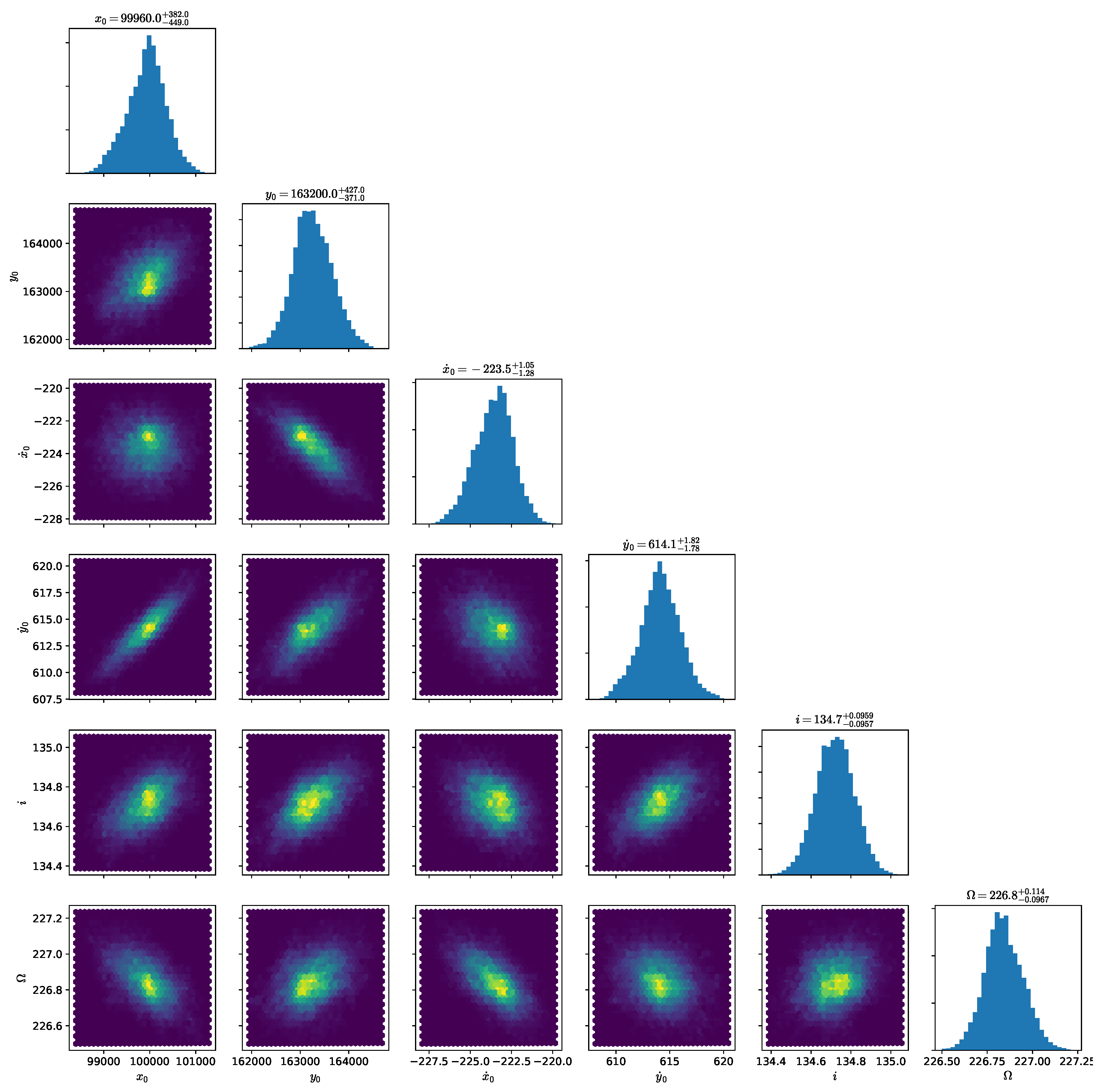
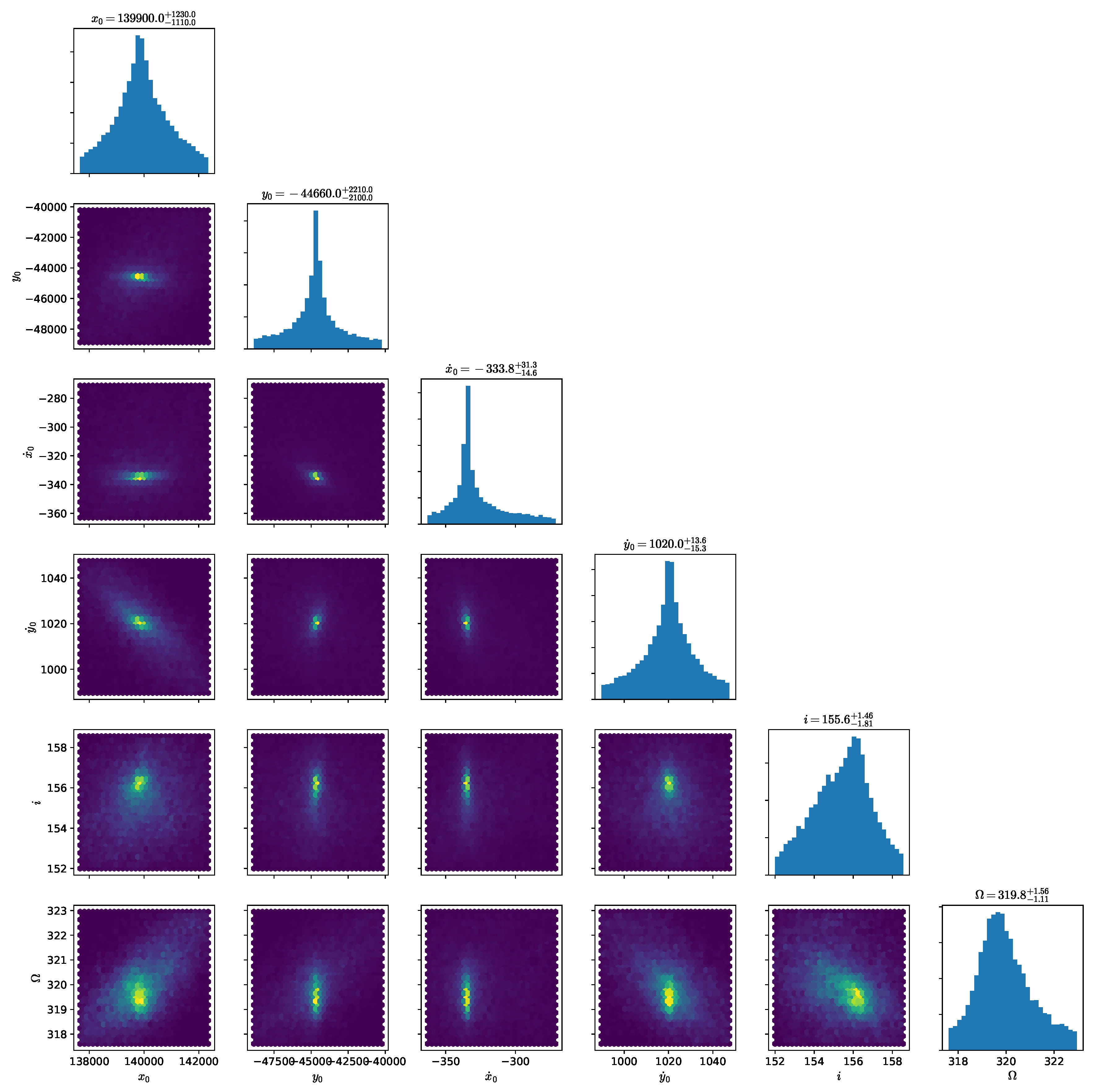
The posterior distributions of S2, S38, S55, and reference frames offsets are presented in the Figure A1–Figure A4 respectively.
Figure A1.
The posterior distribution of the orbital parameters of the S2 star. The initial position vector components are given in the units of the gravitational radius corresponding to the mass of (which is 1,476,625 km). The initial velocity components are given in . The inclination i and the longitude of the ascending node are given in degrees.

Figure A2.
The posterior distribution of the orbital parameters of the S38 star. The units are the same as in Figure A1.
Figure A2.
The posterior distribution of the orbital parameters of the S38 star. The units are the same as in Figure A1.

Figure A3.
The posterior distribution of the orbital parameters of the S55 star. The units are the same as in Figure A1.
Figure A3.
The posterior distribution of the orbital parameters of the S55 star. The units are the same as in Figure A1.

Figure A4.
The posterior distribution of the position of Sgr A* and reference frames offsets. All values are given in the units of mass.
Figure A4.
The posterior distribution of the position of Sgr A* and reference frames offsets. All values are given in the units of mass.

References
- Ghez, A.M.; Salim, S.; Weinberg, N.N.; Lu, J.R.; Do, T.; Dunn, J.K.; Matthews, K.; Morris, M.R.; Yelda, S.; Becklin, E.E.; et al. Measuring Distance and Properties of the Milky Way’s Central Supermassive Black Hole with Stellar Orbits. Astrophys. J. 2008, 689, 1044–1062. [Google Scholar] [CrossRef] [Green Version]
- Genzel, R.; Eisenhauer, F.; Gillessen, S. The Galactic Center massive black hole and nuclear star cluster. Rev. Mod. Phys. 2010, 82, 3121–3195. [Google Scholar] [CrossRef]
- Gillessen, S.; Eisenhauer, F.; Trippe, S.; Alexand er, T.; Genzel, R.; Martins, F.; Ott, T. Monitoring Stellar Orbits Around the Massive Black Hole in the Galactic Center. Astrophys. J. 2009, 692, 1075–1109. [Google Scholar] [CrossRef] [Green Version]
- Gillessen, S.; Plewa, P.M.; Eisenhauer, F.; Sari, R.; Waisberg, I.; Habibi, M.; Pfuhl, O.; George, E.; Dexter, J.; von Fellenberg, S.; et al. An Update on Monitoring Stellar Orbits in the Galactic Center. Astrophys. J. 2017, 837, 30. [Google Scholar] [CrossRef] [Green Version]
- Iorio, L. The short-period S-stars S4711, S62, S4714 and the Lense-Thirring effect due to the spin of Sgr A*. arXiv 2020, arXiv:2009.01158. [Google Scholar]
- Debono, I.; Smoot, G.F. General Relativity and Cosmology: Unsolved Questions and Future Directions. Universe 2016, 2, 23. [Google Scholar] [CrossRef]
- Will, C.M. Theory and Experiment in Gravitational Physics, 2nd ed.; Cambridge University Press: Cambridge, UK, 2018. [Google Scholar] [CrossRef]
- Misner, C.; Thorne, K.; Wheeler, J. Gravitation; Freeman and Co: San Francisco, CA, USA, 1973; p. 891. [Google Scholar]
- Bertotti, B.; Iess, L.; Tortora, P. A test of general relativity using radio links with the Cassini spacecraft. Nature 2003, 425, 374–376. [Google Scholar] [CrossRef]
- Shapiro, I.I. Fourth Test of General Relativity. Phys. Rev. Lett. 1964, 13, 789–791. [Google Scholar] [CrossRef]
- Iorio, L. Calculation of the Uncertainties in the Planetary Precessions with the Recent EPM2017 Ephemerides and their Use in Fundamental Physics and Beyond. Astron. J. 2019, 157, 220. [Google Scholar] [CrossRef] [Green Version]
- Pitjeva, E.V.; Pitjev, N.P. Masses of the Main Asteroid Belt and the Kuiper Belt from the Motions of Planets and Spacecraft. Astron. Lett. 2018, 44, 554–566. [Google Scholar] [CrossRef] [Green Version]
- Park, R.S.; Folkner, W.M.; Konopliv, A.S.; Williams, J.G.; Smith, D.E.; Zuber, M.T. Precession of Mercury’s Perihelion from Ranging to the MESSENGER Spacecraft. Astron. J. 2017, 153, 121. [Google Scholar] [CrossRef]
- Genova, A.; Mazarico, E.; Goossens, S.; Lemoine, F.G.; Neumann, G.A.; Smith, D.E.; Zuber, M.T. Solar system expansion and strong equivalence principle as seen by the NASA MESSENGER mission. Nat. Commun. 2018, 9, 289. [Google Scholar] [CrossRef] [PubMed] [Green Version]
- Deng, X.M. The second post-Newtonian light propagation and its astrometric measurement in the solar system. Int. J. Mod. Phys. D 2015, 24, 1550056. [Google Scholar] [CrossRef] [Green Version]
- Deng, X.M. The second post-Newtonian light propagation and its astrometric measurement in the Solar System: Light time and frequency shift. Int. J. Mod. Phys. D 2016, 25, 1650082. [Google Scholar] [CrossRef]
- Sanghai, V.A.A.; Clifton, T. Post-Newtonian cosmological modelling. Phys. Rev. D 2015, 91, 103532. [Google Scholar] [CrossRef] [Green Version]
- Landau, L.D.; Lifshitz, E.M. The Classical Theory of Fields; Pergamon: Oxford, UK, 1971. [Google Scholar]
- Baryshev, Y. Foundation of relativistic astrophysics: Curvature of Riemannian Space versus Relativistic Quantum Field in Minkowski Space. arXiv 2017, arXiv:1702.02020. [Google Scholar]
- Feynman, R.; Morinigo, F.; Wagner, W. Feynman Lectures on Gravitation; Addison-Wesley Publ. Comp.: Boston, MA, USA, 1995; p. 280. [Google Scholar]
- Baryshev, Y. Translational Motion of Rotating Bodies and Tests of the Equivalence Principle. Gravit. Cosmol. 2002, 8, 232–240. [Google Scholar]
- Preto, M.; Saha, P. On post-Newtonian orbits and the Galactic-center stars. Astrophys. J. 2009, 703, 1743. [Google Scholar] [CrossRef] [Green Version]
- Parsa, M.; Eckart, A.; Shahzamanian, B.; Karas, V.; Zajaček, M.; Zensus, J.A.; Straubmeier, C. Investigating the relativistic motion of the stars near the supermassive black hole in the galactic center. Astrophys. J. 2017, 845, 22. [Google Scholar] [CrossRef] [Green Version]
- Saida, H.; Nishiyama, S.; Ohgami, T.; Takamori, Y.; Takahashi, M.; Minowa, Y.; Najarro, F.; Hamano, S.; Omiya, M.; Iwamatsu, A.; et al. A significant feature in the general relativistic time evolution of the redshift of photons coming from a star orbiting Sgr A*. Publ. Astron. Soc. Jpn. 2019, 71, 126. [Google Scholar] [CrossRef]
- Gainutdinov, R.I. PPN motion of the S-stars around Sgr A. Astrophysics 2020, 63. in print. [Google Scholar]
- Peißker, F.; Eckart, A.; Parsa, M. S62 on a 9.9 yr Orbit around SgrA*. Astrophys. J. 2020, 889, 61. [Google Scholar] [CrossRef]
- Fragione, G.; Loeb, A. An upper limit on the spin of SgrA* based on stellar orbits in its vicinity. arXiv 2020, arXiv:2008.11734. [Google Scholar] [CrossRef]
- Boehle, A.; Ghez, A.M.; Schödel, R.; Meyer, L.; Yelda, S.; Albers, S.; Martinez, G.D.; Becklin, E.E.; Do, T.; Lu, J.R.; et al. An improved distance and mass estimate for Sgr A* from a multistar orbit analysis. Astrophys. J. 2016, 830, 17. [Google Scholar] [CrossRef]
- Chu, D.S.; Do, T.; Hees, A.; Ghez, A.; Naoz, S.; Witzel, G.; Sakai, S.; Chappell, S.; Gautam, A.K.; Lu, J.R.; et al. Investigating the Binarity of S0-2: Implications for Its Origins and Robustness as a Probe of the Laws of Gravity around a Supermassive Black Hole. Astrophys. J. 2018, 854, 12. [Google Scholar] [CrossRef] [Green Version]
- Do, T.; Hees, A.; Ghez, A.; Martinez, G.D.; Chu, D.S.; Jia, S.; Sakai, S.; Lu, J.R.; Gautam, A.K.; O’Neil, K.K.; et al. Relativistic redshift of the star S0-2 orbiting the Galactic Center supermassive black hole. Science 2019, 365, 664–668. [Google Scholar] [CrossRef] [Green Version]
- Gravity Collaboration. Detection of the Schwarzschild precession in the orbit of the star S2 near the Galactic centre massive black hole. Astron. Astrophys. 2020, 636, L5. [Google Scholar] [CrossRef] [Green Version]
- Brumberg, V. Essential Relativistic Celestial Mechanics; IOP Publishing Ltd.: New York, NY, USA, 1991. [Google Scholar]
- Baryshev, Y.V. The equations of motion of the test particles in the Lorentz-covariant tensor gravity theory. Vestn. Leningr. State Univ. 1986, 1, 113–118. [Google Scholar]
- Damour, T.; Deruelle, N. General relativistic celestial mechanics of binary systems. I. The post-newtonian motion. Ann. l’I.H.P. Phys. Théorique 1985, 43, 107–132. [Google Scholar]
- Lämmerzahl, C.; Ciufolini, I.; Dittus, H.; Iorio, L.; Müller, H.; Peters, A.; Samain, E.; Scheithauer, S.; Schiller, S. OPTIS—An Einstein Mission for Improved Tests of Special and General Relativity. Gen. Relativ. Gravit. 2004, 36, 2373–2416. [Google Scholar] [CrossRef] [Green Version]
- Lucchesi, D.M.; Peron, R. Accurate Measurement in the Field of the Earth of the General-Relativistic Precession of the LAGEOS II Pericenter and New Constraints on Non-Newtonian Gravity. Phys. Rev. Lett. 2010, 105, 231103. [Google Scholar] [CrossRef] [PubMed] [Green Version]
- Iorio, L. Post-Keplerian effects on radial velocity in binary systems and the possibility of measuring General Relativity with the star S2 in 2018. Mon. Not. R. Astron. Soc. 2017, 472, 2249–2262. [Google Scholar] [CrossRef] [Green Version]
- Rackauckas, C.; Nie, Q. Differentialequations.jl–a performant and feature-rich ecosystem for solving differential equations in julia. J. Open Res. Softw. 2017, 5. [Google Scholar] [CrossRef] [Green Version]
- Bezanson, J.; Edelman, A.; Karpinski, S.; Shah, V.B. Julia: A fresh approach to numerical computing. SIAM Rev. 2017, 59, 65–98. [Google Scholar] [CrossRef] [Green Version]
- Pfuhl, O.; Gillessen, S.; Eisenhauer, F.; Genzel, R.; Plewa, P.M.; Ott, T.; Ballone, A.; Schartmann, M.; Burkert, A.; Fritz, T.K.; et al. The Galactic Center cloud G2 and its gas streamer. Astrophys. J. 2015, 798, 111. [Google Scholar] [CrossRef] [Green Version]
Publisher’s Note: MDPI stays neutral with regard to jurisdictional claims in published maps and institutional affiliations. |
Figure 1.
The posterior distribution of and .

Figure 2.
The posterior distribution of and .

Figure 3.
The best-fit Parameterized Post-Newtonian (PPN) orbits of S2 (blue), S38 (orange), and S55 (green).
Figure 3.
The best-fit Parameterized Post-Newtonian (PPN) orbits of S2 (blue), S38 (orange), and S55 (green).

Figure 4.
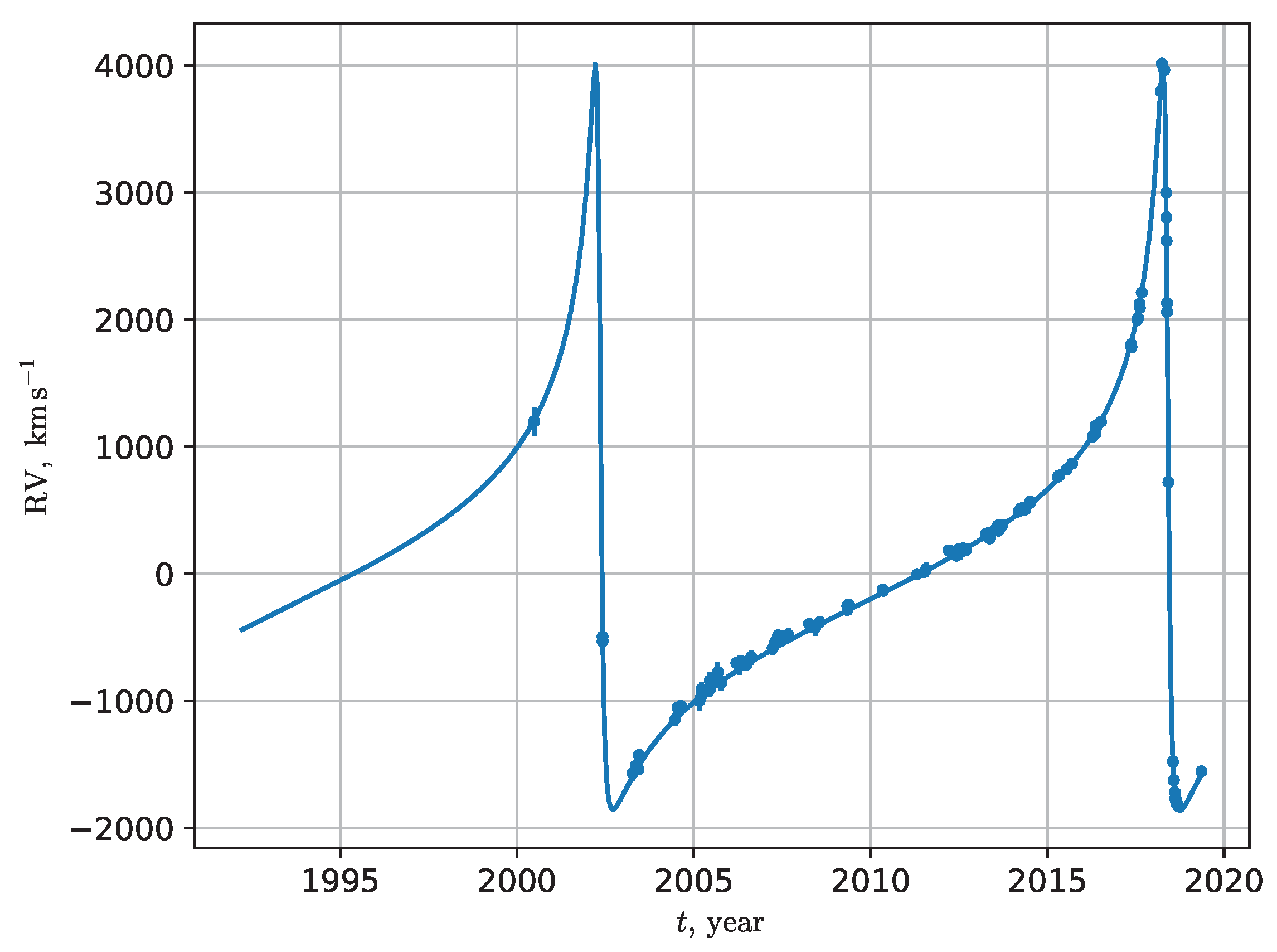
The RV plot of best-fit PPN orbit of S2.

Figure 5.
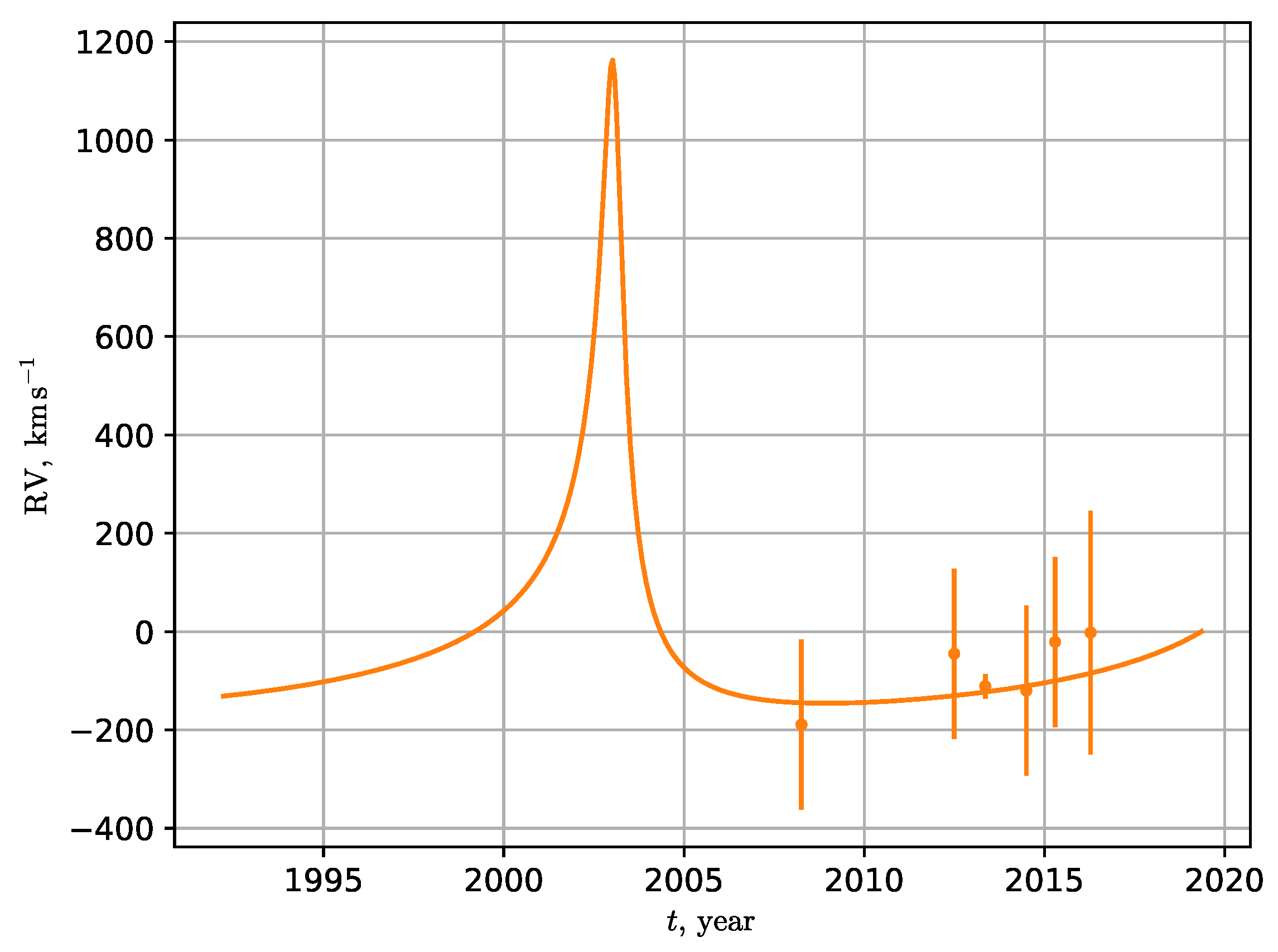
The RV plot of best-fit PPN orbit of S38.

Figure 6.
The RV plot of best-fit PPN orbit of S55.


Table 1.
lS-stars pericenter shift.
| Star | S2 | S38 | S55 |
|---|---|---|---|
© 2020 by the authors. Licensee MDPI, Basel, Switzerland. This article is an open access article distributed under the terms and conditions of the Creative Commons Attribution (CC BY) license (http://creativecommons.org/licenses/by/4.0/).
Share and Cite
MDPI and ACS Style
Gainutdinov, R.; Baryshev, Y. Relativistic Effects in Orbital Motion of the S-Stars at the Galactic Center. Universe 2020, 6, 177. https://doi.org/10.3390/universe6100177
AMA Style
Gainutdinov R, Baryshev Y. Relativistic Effects in Orbital Motion of the S-Stars at the Galactic Center. Universe. 2020; 6(10):177. https://doi.org/10.3390/universe6100177
Chicago/Turabian StyleGainutdinov, Rustam, and Yurij Baryshev. 2020. "Relativistic Effects in Orbital Motion of the S-Stars at the Galactic Center" Universe 6, no. 10: 177. https://doi.org/10.3390/universe6100177
Note that from the first issue of 2016, this journal uses article numbers instead of page numbers. See further details here.