Article

Study of Clear Air Turbulence Related to Tropopause Folding over the Romanian Airspace

1
Faculty of Physics, University of Bucharest, Str. Atomiștilor 405, Măgurele, RO077125 Ilfov, Romania
2
Remote Sensing Department, National Institute of Research and Development for Optoelectronics INOE2000, Str. Atomiştilor 409, Măgurele, RO077125 Ilfov, Romania
3
Weather Forecasting National Center, National Meteorological Administration, Bucuresti-Ploiesti Ave., No. 97, 013686 Bucharest, Romania
*
Author to whom correspondence should be addressed.
Atmosphere 2020, 11(10), 1099; https://doi.org/10.3390/atmos11101099
Submission received: 15 September 2020 / Revised: 7 October 2020 / Accepted: 9 October 2020 / Published: 14 October 2020
(This article belongs to the Section Meteorology)

Abstract

:
Clear air turbulence (CAT) poses a significant threat to aviation. CAT usually occurs in the lower stratosphere and the upper troposphere. It is generally associated with large scale waves, mountain waves, jet streams, upper-level fronts and tropopause folds. Aircraft can experience CAT when flying in proximity of a tropopause fold. To better understand and diagnose tropopause fold- associated CAT we selected a series of cases from among those reported by pilots between June 2017 and December 2018 in the Romanian airspace. Data on turbulence were used in conjunction with meteorological data, satellite imagery, and vertical profiles. Additionally, a set of indices as Ellrod, horizontal temperature gradient, Dutton, and Brown were computed to diagnose CAT associated with tropopause folding. These indices were also analyzed to test the physics mechanisms that may explain the occurrence of severe turbulence. Results show that out of the 420 cases announced by pilots, severe turbulence was reported in 80 cases of which 13 were associated with tropopause folding.

1. Introduction

Atmospheric turbulence can pose serious problems to aviation. The most hazardous type of turbulence occurs in lower troposphere, affecting take-off/landing procedures (i.e., [1]). In the upper troposphere as well as in the lower stratosphere (UTLS), turbulence manifests as an unexpected, dangerous and often elusive phenomenon, commonly known as clear air turbulence (CAT) [2,3].
The upper troposphere turbulence has a significant impact on the safety of air traffic because it can cause structural damage to aircraft and can lead to passenger injuries and even fatalities. Turbulence can also increase operational costs which are passed on to consumers [4]. For this reasons we must identify the areas most frequently associated with turbulence, and in particular with clear-air turbulence. “Clear-air turbulence (CAT) is defined as the bumps of in-flight aircraft directly induced by small-scale turbulent eddies in free atmosphere within cloud free or stratiform clouds” [5]. Recent studies [2,3] provide exhaustive analysis results regarding aviation operations related to meteorological phenomena. Mazon et al. [2] focus on the relative contributions of meteorological phenomena to weather-related aircraft accidents, between 1967–2010, showing that while turbulence was associated with 66% of the cruise flight accidents and 56% of accidents that occur during descent. CAT accounted for 13% of accidents during cruise flights and 7% of accidents during descent.
Moderate to severe localized turbulence generally occurs in areas characterized by strong wind shear, which may be generated by a variety of phenomena including: jet stream, upper-level fronts, unbalanced flow, mountain waves, thunderstorms and gravity waves [4,6,7,8,9,10]. It is no surprise that certain regions within clouds and thunderstorms are usually turbulent, however, thunderstorm-generated turbulence can extend well cloud boundaries. In such circumstances it is referred to as near-cloud turbulence [11]. Also, the Kelvin Helmholtz instability generated by the strong vertical wind shear on the northern edge of the jet, associated with a jet frontal system can be a major cause for generation of the CAT. [12]
In cloud-free areas, CAT is associated with wind shear, particularly occurring between a jet stream’s core and the surrounding air. In a study of 44 aviation accidents caused by turbulence (i.e., CAT, convection, close to mountain), Kaplan et al. [13] indicated a prevalence of severe accident-producing turbulence within the entrance region of the polar or subtropical jet stream, at the synoptic-scale. Their results showed that the most consistent predictor for turbulence was the upstream curvature of the synoptic-scale flow. In most of the cases studied by Kaplan et al. [13], upward vertical motions, low vorticity and an increase of wind shear in time were observed (i.e., conditions associated with the entrance and exit regions of the polar and subtropical jet stream). Recent advancements such as those regarding Doppler LIDAR turbulence measurements [14] have not yet led to a complete explanation of this type of turbulence [15]. Observational studies have indicated that CAT can be caused by Kelvin–Helmholtz instability [16] or that gravity waves (e.g., generated by airflow over mountains) can increase wind shear locally and thus contributing to the generation of CAT [17].
As CAT occurs in cloud-free areas, ice clouds or higher concentration of water vapor, these can be observed and used as hints, indicating the presence of CAT. CAT is difficult to avoid by pilots because it cannot be observed using satellite or radar imagery, neither through the use of on-board radar [15]. Pilots must instead rely on reports of turbulence from preceding flights or CAT forecasting methods such as the graphical turbulence guidance (GTG). GTG uses the output from a numerical weather prediction model to derive several turbulence diagnostics, which are then combined, and the result is validated by the pilot’s reports of turbulence during flight [18]. A third option for CAT prediction is to utilize water vapor imagery, numerical weather prediction models and radar data to detect regions in which tropopause folds occur. Tropopause folds are extrusions of stratospheric air into the troposphere, occurring near an upper-level frontal zone beneath the polar and subtropical jet streams. An aircraft will experience CAT when flying in the proximity of a tropopause fold [5,19]. To our knowledge, there are no pertinent studies concerning CAT over the south-eastern European airspace, and in particular the Romanian airspace. This study aims to detect CAT areas by accounting for the presence of tropopause folds and by computing four indices (e.g., [20,21]) which have been previously used as CAT indicators. These indices were calculated for 13 of CAT cases, namely those for which diagnostic was found to have a direct or indirect link with tropopause folds. These 13 cases were selected from those turbulence cases reported by aircraft pilots, between June 2017 and December 2018, in the Romanian airspace.
Our study shows that of the four indices analyzed, only two can be considered relevant markers for the presence of CAT associated with tropopause folds: the horizontal temperature gradient ( H T ) and the Brown index. The present article is structured as follows: Section 2 details the main aspects of tropopause folds and CAT detection. Section 3 describes the datasets and the methodology used in this article to identify CAT and indices that could be used in CAT associated with tropopause folds. Section 4 presents the results of the performance of turbulence indices and the validation with pilot weather reports or aircraft air-reports (AIREP). The relationship between tropopause folds and prone areas for CAT is detailed for three cases. Finally, Section 5 summarizes the results of this article.

2. Theoretical Considerations on Tropopause Folds and Tropopause Folds Detection

In general, CAT is observed horizontally over distances of 80–500 km in the along-wind direction and 20–100 km in the across-wind direction. Vertical dimensions are 500–1000 m and the life span of CAT is between 30 min and 24 h [22]. CAT can occur in areas with strong horizontal and/or vertical wind shear. Wind shear is most intense on the side of the jet stream with the lowest temperatures, the underside of the jet stream, and on the area between the jet stream and the tropopause. Even if clear-air turbulence is related to the jet stream, not all jet streams contain CAT [22,23]. CAT also can be explained by the Kelvin-Helmholtz instability (KHI). KHI occurs in stably stratified shear flow when the local Richardson number is lower than 0.25 [5]. These conditions are favored by strong wind shear and a large stability [5].
Many cases of CAT occur in areas with strong horizontal and/or vertical wind shear. Wind shear is most intense on the side of the jet stream with the lowest temperatures, the underside of the jet stream, and on the area between the jet stream and the tropopause. Roughly 60% of CAT reports are near jet streams. Clear-air turbulence is often related to the jet stream, but not all jet streams contain CAT [22]. Detection of CAT has to be based on its causes (e.g., tropopause folds, mountain waves, fronts, jet streams). Here we only focus on the detection of CAT associated with tropopause folds.

2.1. Tropopause Folds

Tropopause folds are extrusions of stratospheric air into the troposphere occurring near an upper-level frontal zone beneath the polar and subtropical jet streams [19,24]. 
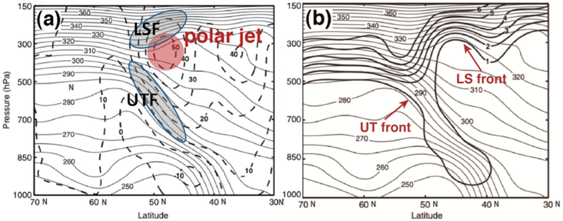
Figure 1a shows a strong polar jet core above a cold front at the surface. In this case, the potential vorticity (PV) contours intrude deep into the troposphere from the stratosphere (Figure 1b). As high values of PV are markers of stratospheric air, the surface of 1.5 or 2 PVU (1 PVU = 1.0 × 10⁻⁶ m2 s−1K kg−1) is considered the dynamic tropopause and its topography is used to identify tropopause folds [25].
Synoptic scale disturbances tend to develop preferentially in regions where the temporal average of maximum zonal wind is associated with jets. Planetary flow in the zone of jet stream has an extremely high degree of baroclinicity [26].
The potential temperature field shows that the lower stratosphere is characterized by higher static stability compared with the upper troposphere. This makes stratospheric air above the lower, polar air mass tropopause, warmer than the stratospheric air above the higher, tropical air mass tropopause, thus creating a discontinuity in the potential temperature field on isobaric surfaces (Figure 1a,b). Berggren [28] proposed and Shapiro [29] confirmed the existence of these frontal-scale transitions within the lower stratosphere [29], later referred by Lang and Martin [27] as lower stratospheric fronts (LSF). In upper level jet-front (ULJF) systems, the LSF is associated with the upper tropospheric front (UTF), both encompassing the jet stream core, as in Figure 1a [27]. As the isentropes cross the tropopause in the vicinity of the jet, there is a mass change between the troposphere and the stratosphere (Figure 1b). In this region (i.e., upper troposphere and lower stratosphere, UTLS) the vertical wind shear associated with the jet stream together with the ageostrophic convergence of polar, subtropical and stratospheric air results in tropopause folding (i.e., a downward intrusion of stratospheric air into the troposphere), a region usually associated with CAT [30]. Tropopause folds are marked by gradients of potential vorticity (PV). PV is a convenient conservative tracer for stratospheric air, but the boundaries of high PV areas (PV anomalies) are also indicative of the location of vertical shear, which can lead to turbulence. The vicinity of the polar jet is characterized by large wind shear. The presence of wind shear in a region also characterized by large stability favors KHI. CAT events can also occur associated to upper-level frontogenesis. Kim and Chun [5] showed that turbulence has been reported near tropopause and near the borders of the upper cold front associated to the tropopause fold.

2.2. Algorithms to Detect Tropopause Fold

A series of algorithms have been proposed to detect tropopause folds. Because tropopause folds are characterized by high values of ozone mixing ratio, high PV, and low relative humidity, these algorithms, as indicated by Antonescu et al. [31] are based on in situ measurements (i.e., ozone, temperature, humidity) [22,32,33] or meteorological analyses to derive diagnostic quantities (i.e., PV, Q-vector) [23,25,34,35]. For example, Sprenger et al. [35] used higher-resolution analyses from ECMWF to identify tropopause folds globally. The algorithm identified tropopause folds as areas of multiple crossings of the dynamic tropopause (defined as the 2 PVU surface).
Because the tropopause fold marks the change in the height of the dynamic tropopause and describes the downward intrusion of stratospheric air characterized by high PV and low humidity into the troposphere, on the satellite imagery (i.e., WV imagery) it is marked by gradients in the upper-level moisture. Thus, for satellite data, the algorithm uses the Spinning Enhanced Visible and Infrared Imager (SEVIRI) 6.2 µm channel which is sensitive to upper tropospheric water vapor (WV 6.2 µm), SEVIRI IR channel at 9.7 µm (very useful for ozone detection) and SEVIRI IR 10.8 µm. Another algorithm that uses satellite data is that from NOAA NESDIS–Center for Satellite Application and Research Algorithm version 2.0 [30]. This has been developed to provide a prediction of turbulence associated with tropopause folding (Tropopause Folding Turbulence Prediction, TFTP) [36] and thus to indicate turbulent flight conditions for aircraft. The gradients in WV channel of the Advanced Baseline Imager flown on the GOES-R, are used as an indication of the distribution of folds. A NWP model is then used to constrain these features vertically in the atmosphere. The algorithm provides the lower and upper bounds of the tropopause folds. Once found, vertical boundaries indicate the vertical width of the atmospheric layers prone to tropopause fold-induced CAT. Based on the above, the study used a subjective identification of tropopause folds by the examination of SEVIRI 6.2 µm WV channel imagery.

3. Data and Methods

3.1. Air Reports (AIREP)

AIREPs indicate turbulence intensity as estimated by the pilot. Within the Romanian airspace, AIREPs are transmitted (via voice radio communication) by the air crew to the air traffic services units which then relay them to the meteorological service unit. According to [37] only moderate and severe turbulence (as defined in Table 1) is reported.
Schwart [38] and Sharman et al. [39] have shown that AIREPs suffer from several limitations. In contrast to automated measurements, they are only semi-quantitative, and subjective, because they depend upon the experience and knowledge of the pilot.
At the same time, the intensity of turbulence included in AIREPs must be interpreted with a certain degree of caution, as it is intrinsically aircraft specific. Small aircraft will experience stronger turbulence than a larger aircraft, when flying through an airspace with the same turbulent eddy dissipation rate. Another limitation of the study is that aircraft turbulence forecasts help aircraft avoid flying through suspected regions of strong turbulence [40]. Recent AIREPs from preceding aircraft flying on the same routes are also dispatched to pilots by air traffic controllers for the same purpose [37].

3.2. Identification of Area with CAT Risk

In this article we identify the areas with CAT risk over Romania by considering the mechanisms associated with tropopause folds. To identify the CAT areas over the Romanian Airspace a database was constructed containing all AIREPs, between June 2017 and December 2018, for the severe and moderate cases of turbulence. The database contains 420 AIREPs for severe and moderate cases, 80 cases of severe turbulence (perhaps CAT) for all flight levels of which 50 cases were reported at levels above the flight level FL350.
Although turbulence manifests at small scale (aircraft size), it can be diagnosed from atmospheric air circulation at the synoptic and mesoscale scales. In the absence of records of turbulence encountered directly by aircraft, the atmospheric reanalysis datasets can be used to identify the areas in which the onset of hydrodynamics instability in the atmospheric flow can occur and is maintained, resulting in CAT. Thus, four turbulence indices were calculated the second Ellrod index (TI2) [20], the horizontal temperature gradient ( H T , [41]), Dutton index (E, [42]), and Brown index (Φ, [43]). TI2 is defined [20] as:
T I 2 = S V D E F Δ H
where S V = v z = u z 2 + v z 2 1 / 2 is the vertical wind shear (s−1).
D E F = D S H 2 + D S T 2 1 2 with D S T = u x v y , D S H = v x + u y   and Δ H = u x + v y being the deformation (DEF), stretching deformation (DST), the shearing deformation (DSH) and horizontal divergence (∆H), respectively. As emphasized by Spensberger and Spengler, for a given wind speed, deformation is inversely proportional to the streamlines curvature radius [44].
The horizontal temperature gradient [32] index is given by the magnitude of the horizontal temperature gradient: h T = T x 2 + T y 2 1 2 .
Using the definition of the thermal wind, and applying the geostrophic approximation for the horizontal wind, [22] shows that the horizontal temperature gradient is related with the vertical wind shear:
h T = f c · T g · V z
where fc is the Coriolis parameter (s−1) and g the acceleration of gravity (m s−2). It is well known that this relation explains the formation of the polar jet stream in response to the temperature contrasts along the polar front.
An empirical turbulence index was determined by [42] based on turbulence reports over the North Atlantic and northwest Europe during 1976 as the sum between the horizontal wind shear and the squared vertical wind shear as follows:
E = 1.25 S H + 0.25 S V 2 + 10.5
where S H = u s s y v s s x is the horizontal wind shear in m s−1 per 100 km,
S V = v z = u z 2 + v z 2 1 / 2 is the vertical wind shear m s−1 per km, and s = u 2 + v 2 1 / 2 is horizontal wind speed. The constants were determined by [39] using multiple linear regression. We notice that SH is defined to be positive if the horizontal wind shear is associated with anticyclonic vorticity and negative in areas with cyclonic shear vorticity. Brown [43] also proposed an empirical turbulence index as:
Φ = 0.3 ζ a 2 + D S T 2 + D S H 2 1 2
where ζ a = ζ + f is absolute vorticity, ζ = v x u y and f is the Coriolis frequency.
All four indices were determined using the global numerical weather prediction (NWP) model output as provided by ERA5 hourly reanalysis data ensuring both a high horizontal and vertical resolution (0.25 × 0.25 degrees horizontal resolution and 25 hPa vertical resolution) [45]. All the CAT indices are calculated using data model from the top and the bottom of the layer inside which a CAT is reported (e.g., between 225 and 250 hPa) and taking the averages of these values for the particular index in that layer [22]. The cut-off values for severe turbulence thresholds are calculated following Sharman et al. [18]. We start by computing the turbulence indices values for each of the 80 severe turbulence (diagnosed as CAT) reports between June 2017 and December 2018. Then we took the median value of each index as the threshold for this turbulence intensity category.
To highlight the mechanisms underlying the generation of CAT associated with the tropopause folds, three events were analyzed (i.e., 4 September 2017, 1 April 2018, and 24 October 2018). The mesoscale and synoptic context of all three events were assessed using ERA5 hourly data on single pressure levels provided by Copernicus Climate Change Service (climate.copernicus.eu). The parameters used were mean sea level pressure (MSLP), 850 hPa temperature, 300 hPa geopotential heights and temperature, 300 hPa wind and potential vorticity on 2.5° × 2.5° horizontal resolution. Vertical cross-sections of temperature, potential temperature, relative humidity, potential vorticity, ozone mass mixing ratio and winds were also taken into consideration within the turbulence areas.

3.3. Identification of Tropopause Folds

The CAT risk areas associated with tropopause folds in Romanian airspace were subjectively identified as follows. First, we used synoptic charts and satellite imagery (WV 6,2 and Air Mass RGB) to visualize jet, PV anomaly and tropopause fold position. Second, it was taking into account that, according to [20] the confluence zone of the polar and subtropical jet-stream branches is a favorable place for CAT. According to Roach and Bysouth [46] CAT usually occurs in layers of strong wind shear below and above the cores of temperate-latitude and subtropical jet streams. We also compared the schema in Figure 2 with the 300 hPa geopotential analysis to find areas with potential for CAT whilst looking for cloud patterns typical of CAT in satellite images. Four turbulence related indices were calculated to find the most relevant ones for tropopause folds-induced CAT.

4. Results

The analysis of the 80 AIREP reports for severe and moderate turbulence showed that 13 reports (16% of all reports) were associated with tropopause folds. Of these, one report was during winter (DJF), two during summer (JJA), six during spring (MAM), and four during autumn (SON). In a study on the role of tropopause folds in summertime tropospheric ozone over the eastern Mediterranean and the Middle East, Akritidis et al. [48] indicated that 3% of all identified tropopause folds between 1979 and 2013 occurred during summer over Romania.
In this study, a summary of the characteristics of the severe turbulence reports associated with tropopause folds was presented in Table 2. For the 13 AIREP reports associated with tropopause fold induced CAT four indices were calculated, according to Section 3.2: TI2, E, H T , and Brown (Table 2).
We selected indices that provide values higher than the calculated threshold on the subset of 13 TF (tropopause folding) cases. Our study shows that in 10 out of 13 (77%) TF events are associated to horizontal thermal gradient exceeding the severe turbulence threshold events followed by the Brown index showing values higher than severe turbulence threshold in eight out of 13 (62%) cases (Table 2). Dutton and Ellrod TI2 indices exhibit values higher than severe turbulence threshold in only 54% and 31% respectively of tropopause folding-induced CAT. Our results suggest that   H T and the Brown index could be used as proxies for tropopause fold induced CAT, being thus of real use in the aeronautical forecast of this CAT type.

4.1. Case Studies

To highlight meteorological conditions associated with CAT risk area in complex orography of Romanian airspace, three events with severe turbulence, reported by the pilots were analyzed in detail.

4.1.1. Case Study 4 September 2017

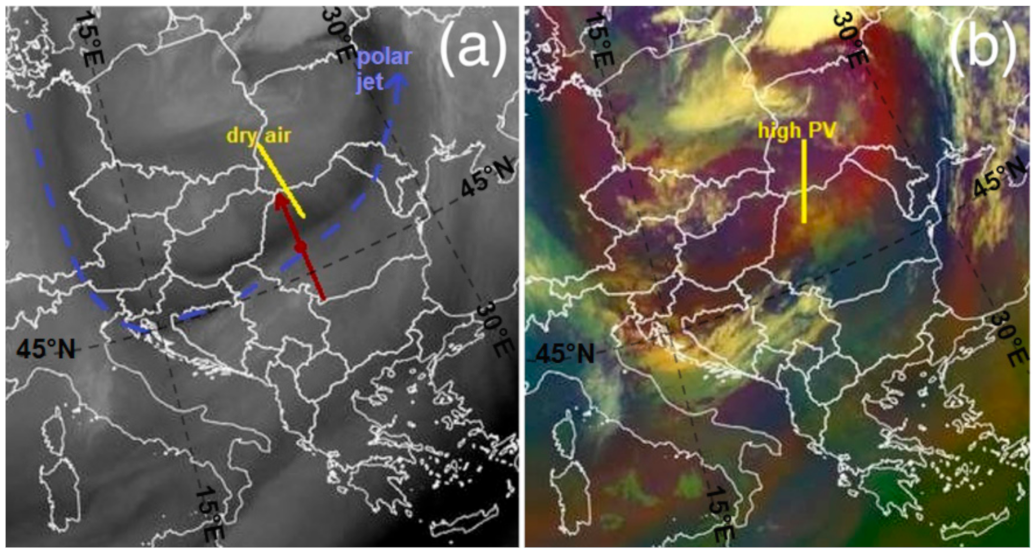
On 4 September 2017 at 21:11 UTC, pilots reported severe turbulence at FL 370 (11,300 m altitude and 216 hPa pressure level), at about 45.95°N and 23.08°E, the closest city to the ground being Alba Iulia (in central Romania). The fastest, but not very accurate, method of identifying the conditions for turbulence in the upper atmosphere is satellite imagery analysis. From the water vapor channel satellite image (WV6.2) it appears that the turbulence was reported near the edge of an area of subsiding dry air, in the medium to upper troposphere (dark grey band), and to the southern boundary of a polar jet (Figure 3a).
Furthermore, the reddish color featured by air mass RGB, in the same area, is a sign of ozone-rich descending stratospheric air, to lower and warmer levels (Figure 3b). Stratospheric intrusions are associated with high potential vorticity anomalies [31] and typically occur poleward of the jet stream axis in tropopause folds [6], as in this case. This situation is one in which a meteorologist can expect turbulence to occur and most likely this turbulence is CAT.
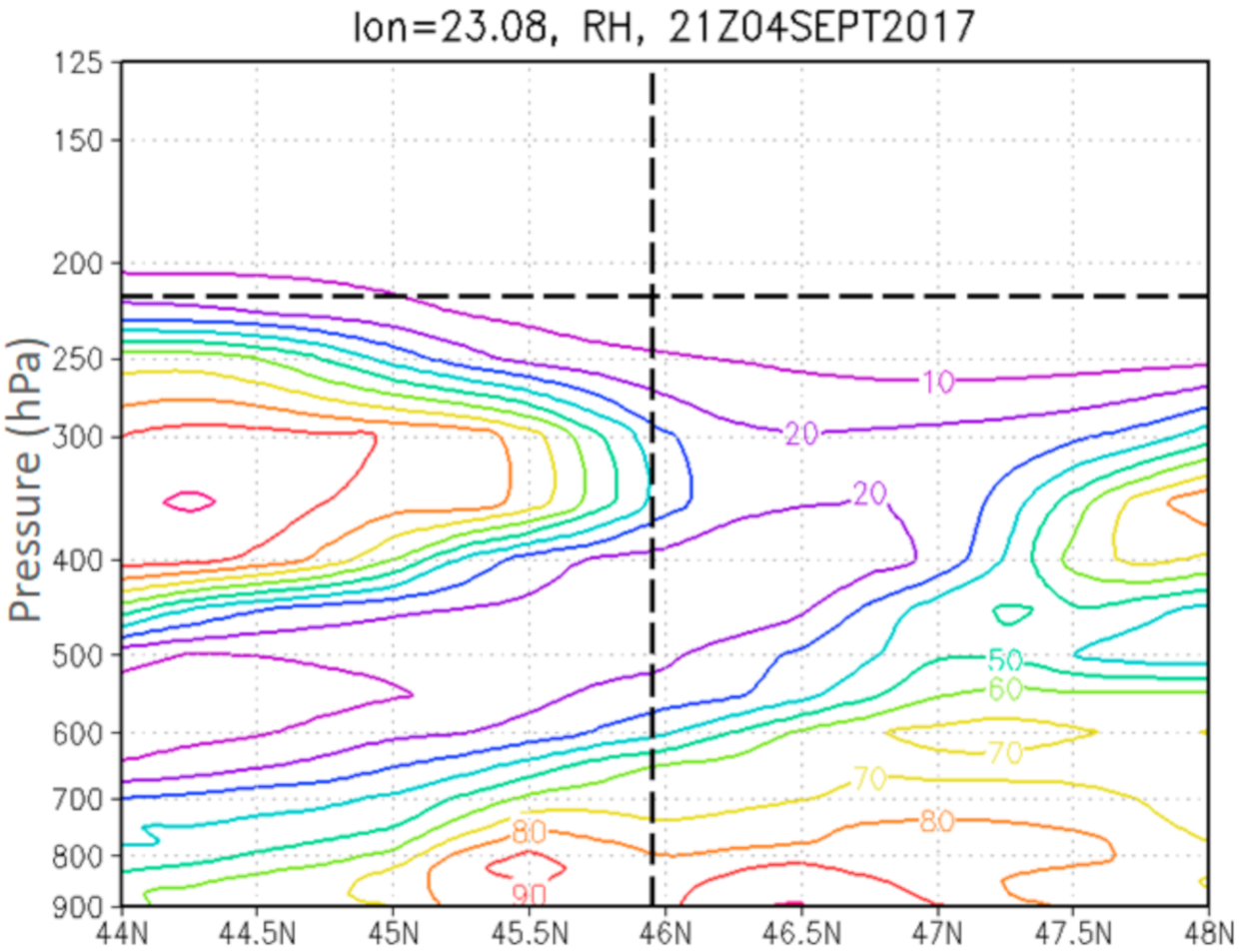
At the coordinates where turbulence was reported, the relative humidity is low (<20%) (Figure 4). Below this level the humidity was rising, and most likely suggests the presence of stratiform clouds. Above these clouds the air was dry and the sky clear.
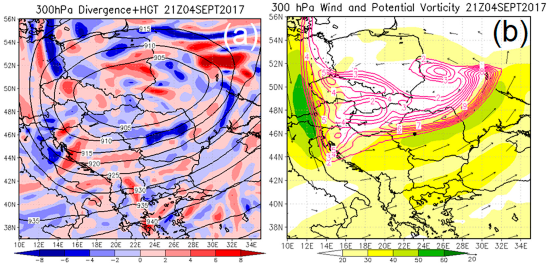
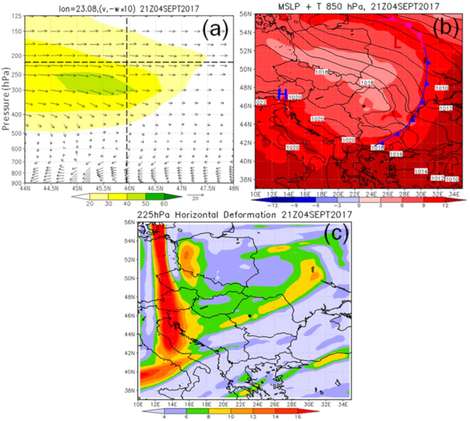
To the NNW of Romania, a cut-off low, extended to the upper troposphere, was inducing an intense WSW circulation at 300 hPa above northern Balkans. (Figure 5a) A polar jet streak was situated over Romania and the severe turbulence occurred immediately poleward of its axis (Figure 5b), an area favorable to this type of phenomenon (J area from Figure 2). Moreover, Figure 5b shows that the event occurs at the southern edge of a positive PV anomaly.
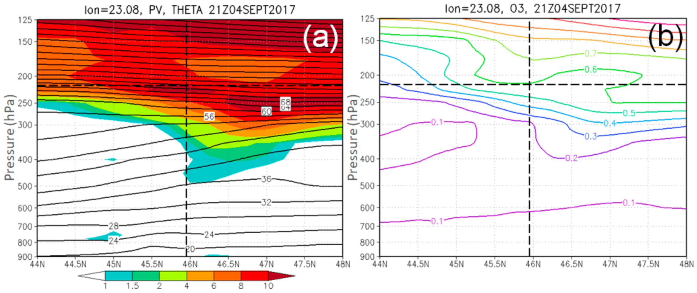
The surface of 1.5 PVU (dynamical tropopause) dropped to around the 400 hPa level (Figure 6a). The ozone concentration longitudinal cross section near 23°E shown in Figure 6b, confirms the presence of a tropopause fold, i.e., values over 0.2 ppm above 400 hPa level north of 46°N (see also [49]).
The maximum wind speed at 200 hPa (the altitude of the reported turbulence) clearly shows the upper trough stretching NE-SW over north-western Romania, wind speed exceeding 40 m s−1 above the reported point (Figure 5b and Figure 7a). The color gradient (yellow to green) shows a significant amount of both horizontal and vertical wind shear, implying that turbulence can result.
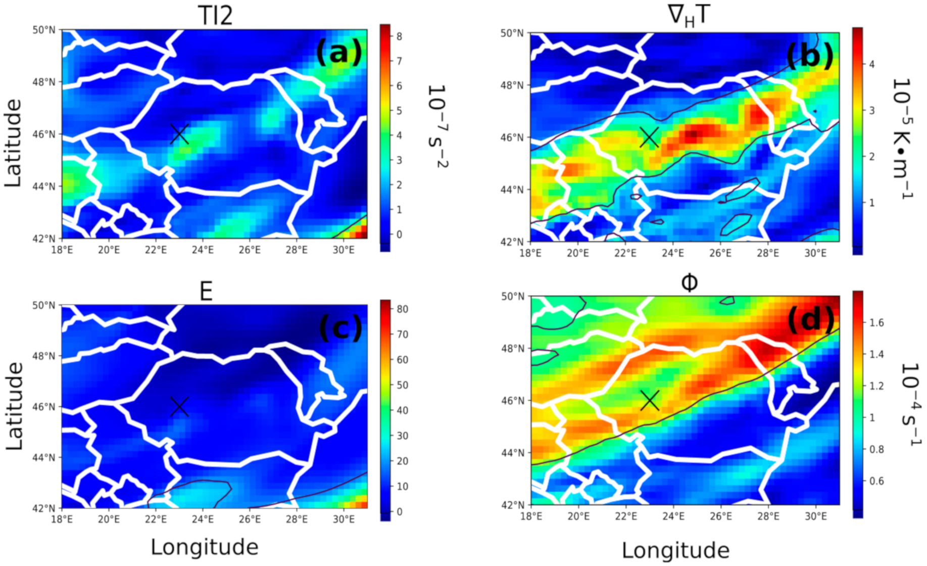
Figure 8 depicts the four turbulence indices fields over Romania for the 4 September 2017 at 21:00 UTC. On the one hand, over the region of interest, both TI2 and E show values well below the severe turbulence thresholds (Table 2). On the other hand, H T exceeds the severe threshold value, indicating turbulence producing conditions within a delimited continuous SW–NE orientated band. The Brown index (Φ) suggests a wider area of turbulence comprising the entire northern region (Figure 8d). These results are in agreement with the presence of a frontal zone in the upper troposphere (Figure 6a), on a rearward sloping cold front moving to south-east (Figure 7b) and also with a band of high cyclonic relative vorticity poleward of the SW-NE orientated jet stream (Figure 5b and Figure 7a); the latter corresponds to the potential vorticity anomaly within the tropopause fold (Figure 5b).
The horizontal thermal gradient ( H T ) at the turbulence report level is associated to the LSF, having an opposite sign to the UTF temperature gradient (see Figure S1 in the Supplementary Material) (e.g., [27,45]). North of 46°N, above the tropopause fold, the thicker more stable stratospheric air is warmer than the air outside the tropopause fold on the same isobaric surfaces, thus creating a warm stratospheric pool inside the fold. This, in turn, leads to a reversal of the thermal wind direction above the tropopause which generates vertical wind shear, due to wind speed rapidly decreasing above the jet core (Figure 7a). Note that this wind shear is at a maximum just south of the report location, above the jet stream axis, contributing, jointly with an upper convergence zone (Figure 5a), to a local maximum of the TI2 marginal to the severe turbulence threshold (Figure 7b).
The low values of the Dutton index in the report area are accounted for by the cyclonic shear vorticity poleward of the jet axis (Figure 7a) which partially offsets the effect of the vertical wind shear. Similarly, the relatively low values of the second Ellrod index outside the mentioned maximum are due to the lower contribution of deformation in areas of horizontally homogeneous, relatively low curvature flow (Figure 7c).

4.1.2. Case Study 1 April 2018

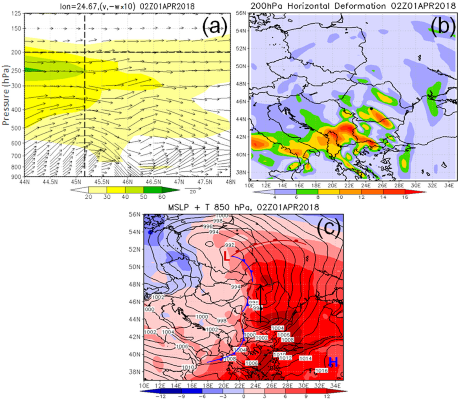
The event of 1 April 2018 occurred at 02:07 UTC, when the pilots reported severe turbulence at FL 390 (12 km altitude and 200 hPa pressure level), at approximately 45.17°N and 24.67°E, the closest city to the ground being Curtea de Argeș, southern Romania.
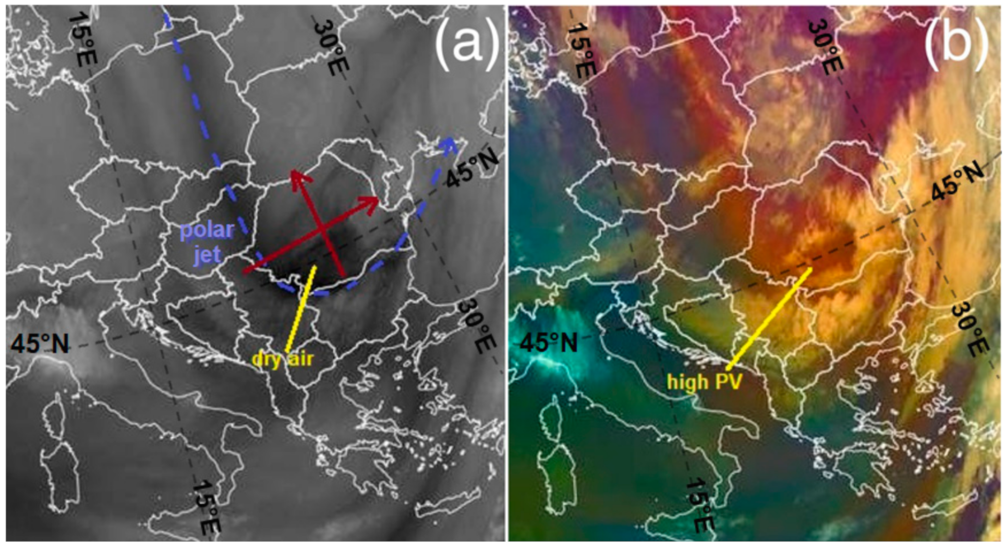
As it can be seen from satellite images (Figure 9), the turbulence occurred above an area with quite a high humidity gradient. In the WV 6.2 μm (Figure 9a) grey and dark grey areas are associated with intrusion of stratospheric dry air, and light grey and white areas indicate more moisture. In the Air mass RGB product, the humidity contrast is clearer between the two bands (one dark brown and the other one whiter). This can be also seen in relative humidity cross-section through the point where the report was transmitted (Figure 10a). The vertical relative humidity cross-section (Figure 10a) reveals that above 300 hPa level the air was very dry.
At 300 hPa level the turbulence report area was ahead of a trough extended from Germany to northern Greece, behind a developing upper ridge (Figure 11a), and on the left exit of a jet streak (Figure 11b). Thus, the turbulence appeared in an area with upper level divergence (similar to the R and D areas from Figure 2).
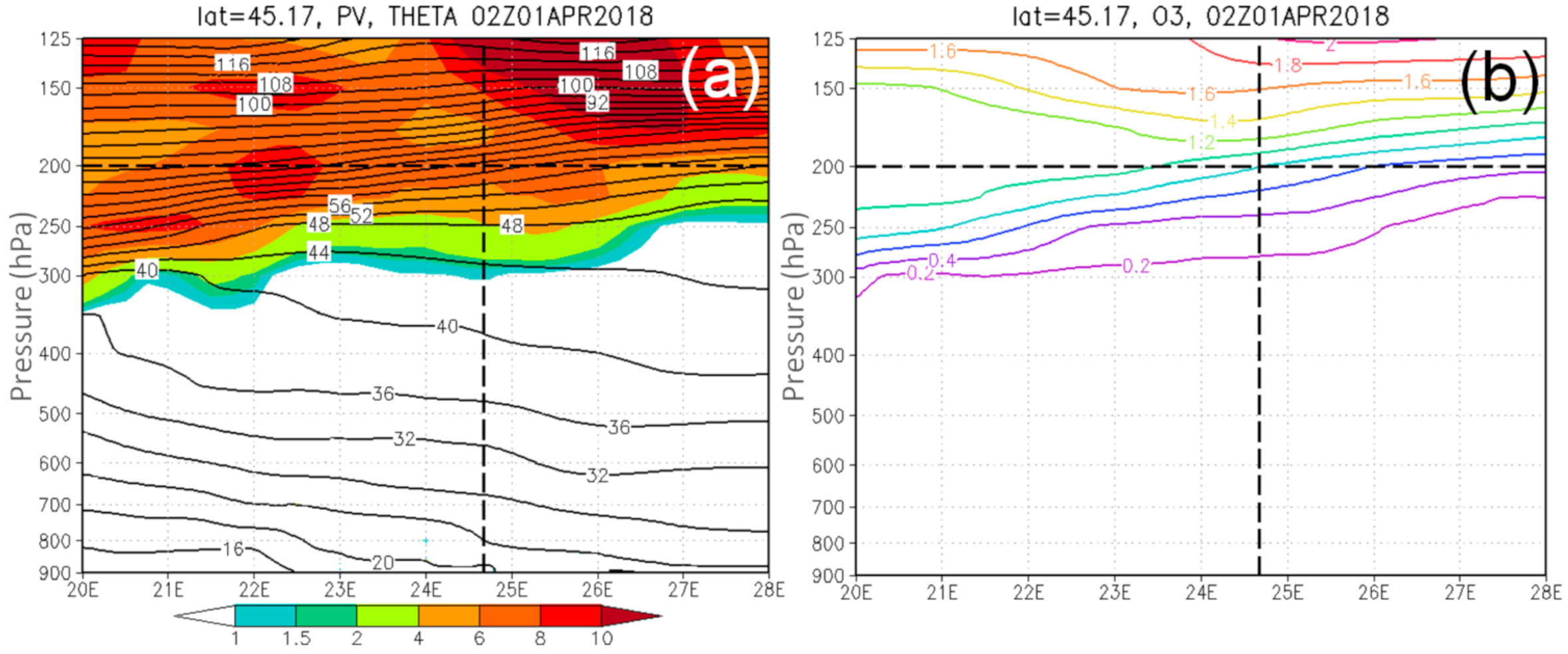
In the area of the reported severe turbulence, the surface of 1.5 PVU was near the 300 hPa level (Figure 12a). An indication of the tropopause level, can also be seen in Figure 12b, in the ozone cross-section. The altitude at which the trubulence was reported (approximately 12 km) was within the stratosphere, in low humidity, cloud free conditions (Figure 9a and Figure 10a), which supports the classification of the event as CAT.
In the South-West of Romania, a high potential vorticity anomaly (Figure 11b) indicated the presence of a tropopause fold, and ahead of this anomaly strong potential vorticity advection over the Romania-Serbia border area (Figure 11b). This was forcing significant large-scale ascent (Figure 10b) within a warm conveyor belt (WCB) structure which is evidenced by the baroclinic leaf cloud formation (Figure 9) and also in the relative humidity zonal vertical cross-section (Figure 10a).
Koch [7] showed that upper tropospheric frontal zones often produce gravity–inertia waves, which propagate into the lower stratosphere within the high shear layer above the tropospheric jet stream. In turn, Shapiro [49] related CAT to PV gradients and Kaplan et al. [13] created a CAT predictor based on relative vorticity gradients. Turbulence may result from weak gravity waves when they modify the environmental stability and wind shear. Therefore, gravity waves are an indirect cause of CAT [50], In our case, the satellite image show a wave pattern within the baroclinic leaf cloud formation in RGB AIRMASS image, clearly seen over western part of Romania (Figure 9b).
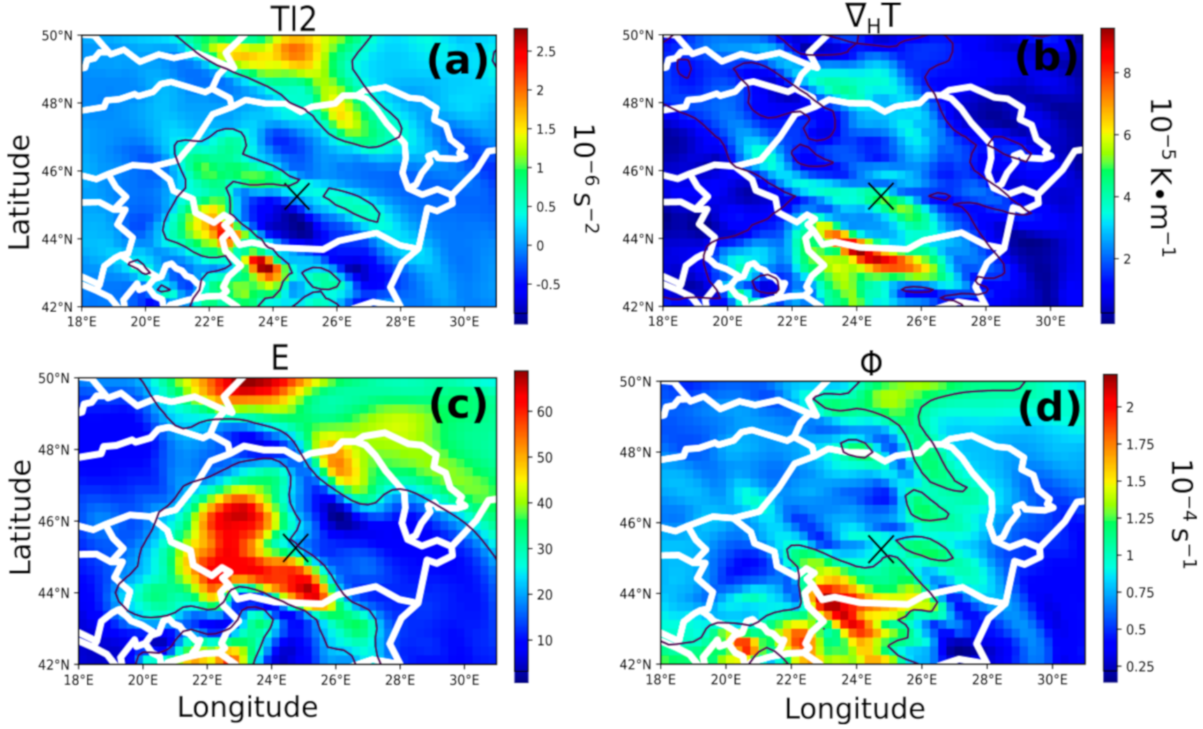
As in the previous case (Section 4.1), the horizontal temperature gradient and subsequent thermal wind reversal (Figure 13a) in the lower stratosphere above the east-west sloping tropopause (Figure 12) leads to increased values of H T (exceeding almost 4 times the threshold for severe CAT) and vertical shear-related indices (E and TI2) at the level of the turbulence report. Furthermore, Dutton index (E) is also favored by the increasingly anticyclonic curvature of the upper flow ahead of the ridge (Figure 14) and by a local deformation maximum associated with a shortwave trough embedded in the southwesterly flow (Figure 11a and Figure 13b). The divergence area ahead of the trough is keeping TI2 at lower values (just below the threshold). Very high values of cyclonic vorticity (through combined shear and curvature contributions) near the axis of the diffluent trough explain the maximum of the Brown index over SW Romania (Figure 14). Although the per se tropopause fold is in this case positioned outside of Romanian territory, the zonal (eastward) sloping of the tropopause associated with a major frontal zone (Figure 13c) influences all the turbulence indicators over large parts of Romania.

4.1.3. Case Study 24 October 2018

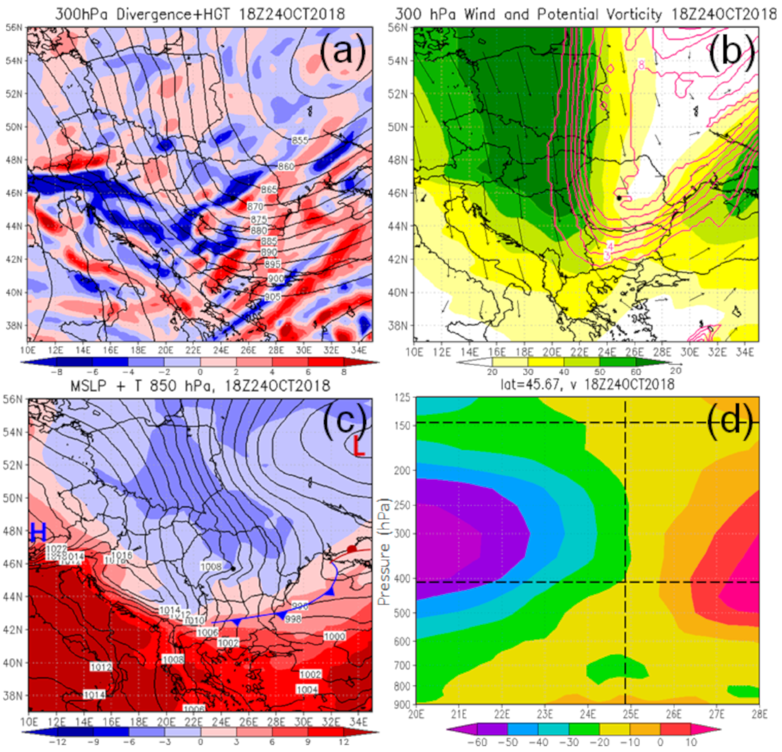
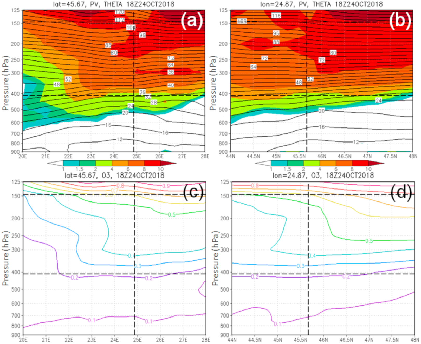
Another case of CAT associated with a tropopause fold occurred on 24 October 2018. Severe turbulence was reported at 1753 UTC, FL 450 (13700 m and 147 hPa pressure level) at approximately 45.67°N, 24.87°E and at 1817 UTC, FL 230 (7000m, 410 hPa pressure level), the closest city for both reports was Făgăraș (in central Romania).
The satellite images reveal that the severe turbulence occurred in an area with few medium clouds (Figure 15a, dark grey area), and a dry stratospheric air intrusion with high positive potential vorticity anomaly (Figure 15b, reddish area). This agrees with the relative humidity meridional vertical cross-section through the observation point (Figure 16). It indicates high humidity up to 500 hPa (low and medium clouds) and dry cloudless air above this level. Thus, turbulence from both reports was classified as CAT.
As shown in Figure 17, the reported severe turbulence occurred on the axis of an upper air trough (a) (T area from Figure 2), and near the eastern boundary of a polar jet branch (b) (J area from Figure 2)-areas in which usually turbulence can occur.
The CAT area lies within a high positive PV anomaly (Figure 17b). The 1.5 PVU surface (dynamic tropopause) descended to the middle of the troposphere (between 500 and 600 hPa level) (Figure 18a,b) indicating the presence of a tropopause fold. The tropopause fold is also indicated in the ozone concentration vertical cross section (Figure 18c,d) which shows a strong transport between the stratosphere and the troposphere.
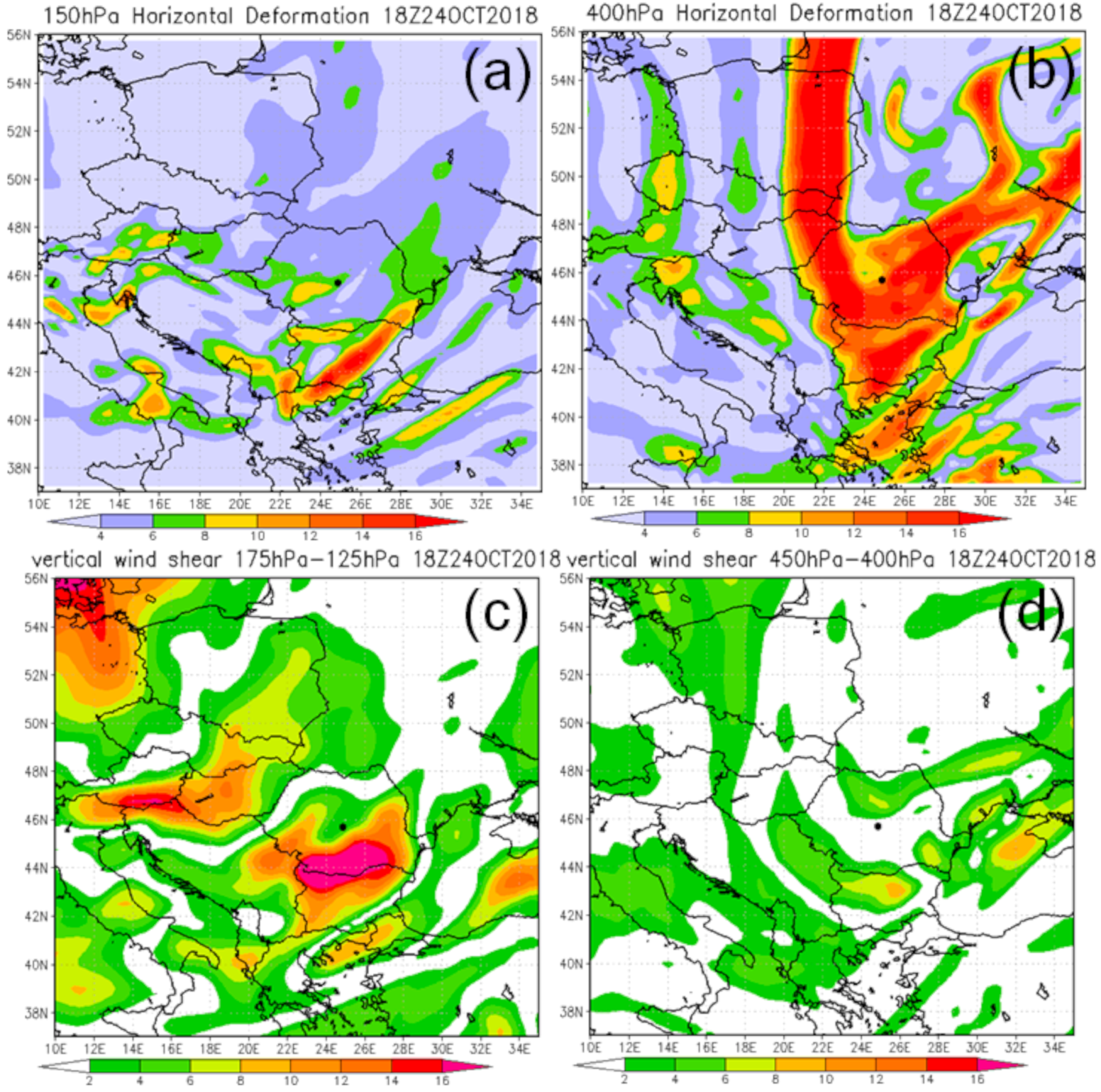
As shown in 
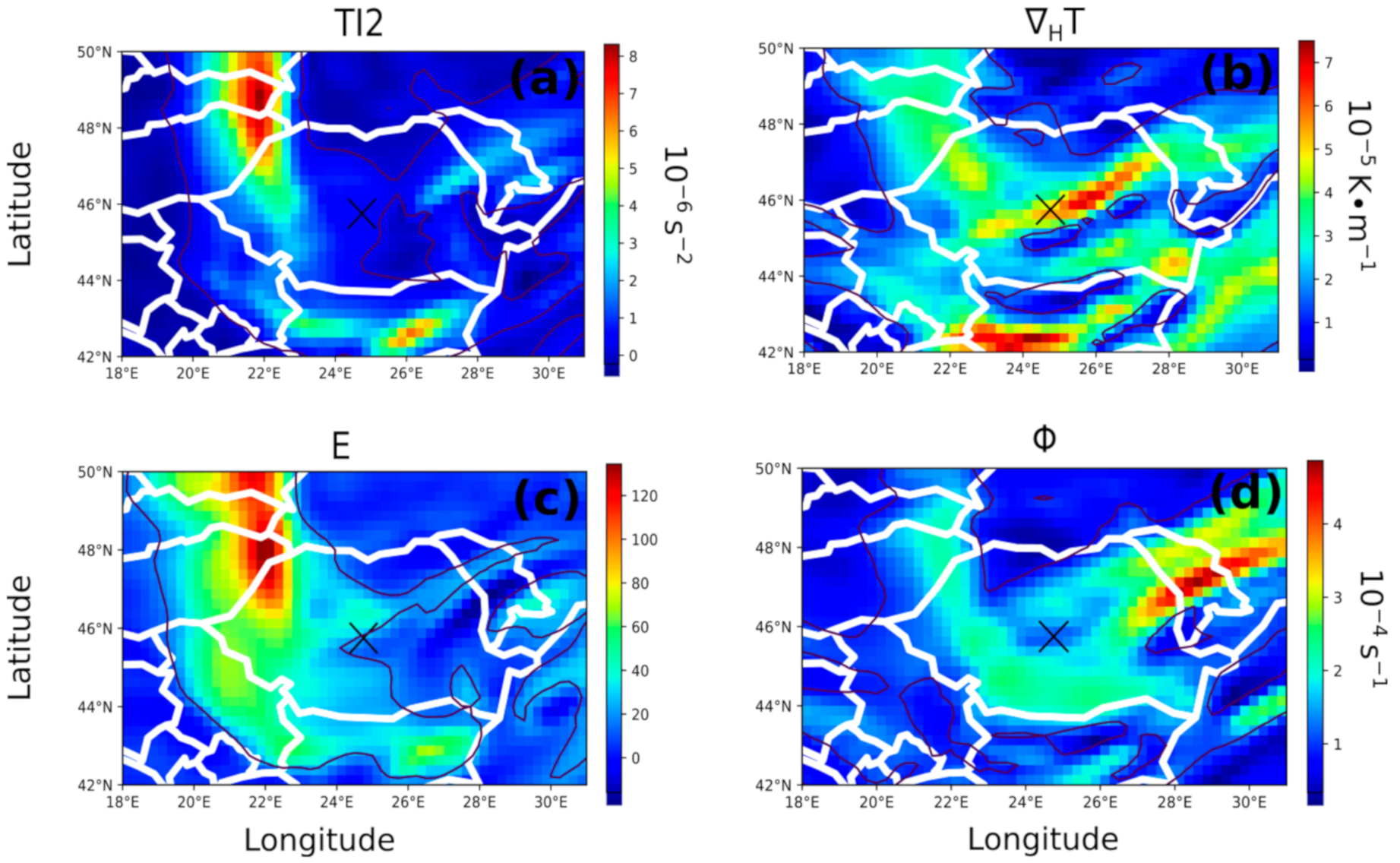
Figure 17c, Romania was behind of a cold front, and MSLP was rising due to strong descending motions caused by the cold advection and negative vorticity advection leading to upper level convergence behind the upper trough axis. In this case, the TI2 maximum is mostly caused by the strong convergence behind the trough axis (Figure 17a) and by the horizontal shear (of the v component) and shearing deformation caused by the flow curvature, especially at the lower report level (Figure 17d and Figure 19a,b), while the maximum of the Brown index-by the high values of vorticity near the trough axis (Figure 17b). As for H T , which exceeds almost three times the threshold value for severe turbulence at the location of the reports (Table 2), it is the result of temperature gradients of opposed signs at the levels of the two reports. As in the previous cases, the marked meridional and zonal slope of the tropopause is causing a reversal of the horizontal temperature gradient from its tropospheric values, with warmer air lying in the lower stratosphere at the upper report level to the North and East (Figure 18a,b). This, in turn, generates a south-easterly thermal wind and provides the vertical shear in the lower stratosphere at or near the upper report location (Figure 19c and Figure 20a,b). Conversely, the horizontal temperature gradient near the lower report location is the tropospheric gradient related to the upper cold front, with warmer air lying to the South (Figure 18a,b).
This generates a westerly thermal wind and corresponding vertical shear near the lower report location (Figure 19d and Figure 20a), but the horizontal shearing deformation around the trough axis appears to be the main factor in this case.
The Dutton (E) index is the only one that presents relatively low values over the reports area, mostly due to the prevalence of cyclonic shear (Figure 21 and Figure 22).
The two reports are thus connected to the shear layers representing the upper and lower boundaries of the tropospheric jet stream and to the stratospheric and tropospheric layers of horizontal temperature gradients forming the upper frontal zones (see also [5,24,27]).

5. Conclusions

Romania is a country with an important role in international air transport, with over 107 thousand jobs in aviation and economic activity exceeding 2.3 billion euros, the 23rd place in Europe [51] Romania’s airspace is very important, since it serves Europe-Asia traffic, with 19.317 million passengers out of a total of over 1.105 billion transiting Europe in 2018 [52]. From this point of view, the study of the meteorological conditions over the Romanian airspace of the country it is important for the safety of international air traffic routes.
Through this study we contribute to a more accessible and faster way of forecasting CAT associated with tropopause folds, based on NWP calculated indices (model diagnostics). To better understand the threat of CAT in the Romanian airspace, pilot reports for turbulence between June 2017 and December 2018 were analyzed. Our study focuses on the influence of tropopause folds on higher than moderate CAT events and is aimed at finding appropriate indices which can be quickly and easily used by meteorological forecast centers.
To analyze CAT events, a series of turbulence indices previously proposed by different authors have been calculated (i.e., Ellrod, Dutton, Brown and horizontal temperature gradient). Reanalysis data and satellite imagery were also used to characterize the environments associated with CAT.
A total of 420 turbulence reports were analyzed, with severe turbulence being reported in 80 cases of which 13 cases where associated with tropopause folding. The results showed that the most useful indices for identifying tropopause folding related CAT are the horizontal temperature gradient and Brown index (77% of TF cases are associated to   H T exceeding severe turbulence threshold and 62% of TF cases showed Brown index exceeding severe turbulence threshold). Thus, these two indices, used together, could offer a good indication of CAT related tropopause folding development for aeronautical forecasters everywhere in Europe and not only.
To give more robustness to our results, three relevant case studies of CAT associated with tropopause fold were analyzed and the main conclusions are:
(1)
In all three cases, the turbulence was reported above the dynamic tropopause, where strong stability provides one of the ingredients for KHI. Horizontal temperature gradients and the related vertical shear induced in the lower stratosphere by tropopause folds or tropopause sloping in frontal zones adds to provide the other KHI ingredient, thus increasing the risk of clear air turbulence, especially when combined with vorticity and/or deformation fields.
(2)
H T is the only one index which present extremely high values in all three case studies presented here. Therefore, this index can be associated to this special case of CAT suggesting that it can be used as a proxy for turbulence originating from tropopause folding.
(3)
All the three cases were located in proximity of a tropospheric jet stream, either polweard of the jet core (case 1), or at its entrance/exit (cases 2 and 3).
As most of the air traffic within the Romanian airspace occurs at high levels (300–150 hPa), when tropopause lowers, the aircraft sample the lower stratosphere, well above the tropopause. Therefore, a complete study of turbulence occurences around the tropopause folds, needs to be based on a large number of air traffic reports within the troposphere. For instance a terminal area of a major airport (e.g., Bucharest Otopeni) where both ascending and descending flights take place in large numbers. For statistical significance, it will need to extend over a longer period of time, due to the more limited spatial extent of the domain sampled by air traffic in this case. Further work is also needed to investigate the use of Richardson number in TF induced CAT and to test the performance of TF induced CAT forecasts.
Nevertheless, the case studies show that tropopause folds and their connected dynamical processes can be the trigger for CAT events well above and away from the tropopause surface.

Supplementary Materials

The following are available online at https://www.mdpi.com/2073-4433/11/10/1099/s1, Figure S1. (a) Vertical-meridional cross-section (40N-55N) of temperature (°C, shaded as indicated on the color bar, every 5°C) through the turbulence report location (starred) at 21 UTC 4 September 2017, showing dynamic tropopause (dark grey line), jet core, warm stratospheric pool and the upper frontal regions: UTF and LSF; (b) Vertical-meridional cross-section (40N-55N) of zonal wind component u (ms-1) through the turbulence report location (starred) at 21 UTC 4 September 2017; (c) 400 hPa temperature (d) 200 hPa temperature-very close to the report level (°C, shaded as indicated on the color bar, every 5°C) at 21 UTC 4 September 2017 (turbulence report location-dot).

Author Contributions

Conceptualization, S.Ș. and B.A.; methodology, S.Ș. software, C.N.; validation, A.D.U., L.B., and M.D.A.; formal analysis, S.Ș.; investigation, A.D.U., M.D.A., L.B., and C.N.; resources L.B.; data curation, M.D.A.; writing—original draft preparation, S.Ș.; writing—review and editing, all the authors; visualization, L.B., M.D.A., C.N., and S.V.; supervision, S.Ș.; funding acquisition, S.Ș. All authors have read and agreed to the published version of the manuscript.

Funding

This work was supported by Partner University of Bucharest, Faculty of Physics grant from the Romanian Ministry of Research and Innovation, CCCDI–UEFISCDI, project number 87PCCDI/2018.

Acknowledgments

This work was supported by a grant from the Romanian Ministry of Research and Innovation, CCCDI–UEFISCDI, project number 87PCCDI/2018, project registration code PN-III-P1-1.2-PCCDI-2017-0868, within PNCDI III from Partner University of Bucharest, Faculty of Physics. The authors gratefully acknowledge ROMATSA for providing some of the data used in this article. We are very grateful to the three anonymous reviewers for their constructive comments and suggestions which significantly improved our manuscript.

Conflicts of Interest

The authors declare no conflict of interest.

References

  1. Maruhashi, J.; Serrão, P.; Belo-Pereira, M. Analysis of Mountain Wave Effects on a Hard Landing Incident in Pico Aerodrome Using the AROME Model and Airborne Observations. Atmosphere 2019, 10, 350. [Google Scholar] [CrossRef] [Green Version]
  2. Mazon, J.; Rojas, J.I.; Lozano, M.; Pino, D.; Prats, X.; Miglietta, M.M. Influence of meteorological phenomena on worldwide aircraft accidents, 1967–2010. Meteorol. Appl. 2018, 25, 236–245. [Google Scholar] [CrossRef]
  3. Gultepe, I.; Sharman, R.; Williams, P.D.; Zhou, B.; Ellrod, G.; Minnis, P.; Feltz, W. A review of high impact weather for aviation meteorology. Pure Appl. Geophys. 2019, 176, 1869–1921. [Google Scholar] [CrossRef]
  4. Sharman, R.D.; Trier, S.B.; Lane, T.P.; Doyle, J.D. Sources and dynamics of turbulence in the upper troposphere and lower stratosphere: A review. Geophys. Res. Lett. 2012, 39. [Google Scholar] [CrossRef] [Green Version]
  5. Kim, J.H.; Chun, H.Y. A numerical study of clear-air turbulence (CAT) encounters over South Korea on 2 April 2007. J. Appl. Meteorol. Clim. 2010, 49, 2381–2403. [Google Scholar] [CrossRef]
  6. Lester, P.F. Turbulence: A New Perspective for Pilots; Jeppesen Sanderson: Englewood, CO, USA, 1993; p. 212. [Google Scholar]
  7. Koch, S.E.; Jamison, B.D.; Lu, C.; Smith, T.L.; Tollerud, E.I.; Girz, C.; Wang, N.; Lane, T.P.; Shapiro, M.A.; Parrish, D.D.; et al. Turbulence and Gravity Waves within an Upper-Level Front. J. Atmos. Sci. 2005, 62, 3885–3908. [Google Scholar] [CrossRef]
  8. Wolff, J.K.; Sharman, R.D. Climatology of upper-level turbulence over the continental Unites States. J. Appl. Meteorol. Climatol. 2008, 47, 2198–2214. [Google Scholar] [CrossRef]
  9. Lane, T.P.; Sharman, R.D.; Trier, S.B.; Fovell, R.G.; Williams, J.K. Recent advances in the understanding of near-cloud turbulence. Bull. Amer. Meteor. Soc. 2012, 93, 499–515. [Google Scholar] [CrossRef] [Green Version]
  10. Kim, J.; Sharman, R.D.; Benjamin, S.G.; Brown, J.M.; Park, S.; Klemp, J.B. Improvement of Mountain-Wave Turbulence Forecasts in NOAA’s Rapid Refresh (RAP) Model with the Hybrid Vertical Coordinate System. Weather Forecast. 2019, 34, 773–780. [Google Scholar] [CrossRef]
  11. Lane, T.P.; Sharman, R.D.; Clark, T.L.; Hsu, H.M. An investigation of turbulence generation mechanisms above deep convection. J. Atmos. Sci. 2003, 60, 1297–1321. [Google Scholar] [CrossRef]
  12. Lee, D.; Chun, H. A Numerical Study of Aviation Turbulence Encountered on 13 February 2013 over the Yellow Sea between China and the Korean Peninsula. J. Appl. Meteor. Climatol. 2018, 57, 1043–1060. [Google Scholar] [CrossRef]
  13. Kaplan, M.L.; Huffman, A.W.; Lux, K.M.; Charney, J.J.; Riordan, A.J.; Lin, Y.L. Characterizing the severe turbulence environments associated with commercial aviation accidents. Part 1: A 44-case study synoptic observational analyses. Meteorol. Atmos. Phys. 2005, 88, 129–152. [Google Scholar] [CrossRef]
  14. Harrison, R.G.; Heath, A.M.; Hogan, R.J.; Rogers, G.W. Comparison of balloon-carried atmospheric motion sensors with Doppler lidar turbulence measurements. Rev. Scient. Inst. 2009, 80, 026108. [Google Scholar] [CrossRef] [PubMed]
  15. Williams, P.; Joshi, M. Intensification of winter transatlantic aviation turbulence in response to climate change. Nat. Clim Chang. 2013, 3, 644–648. [Google Scholar] [CrossRef]
  16. Watkins, C.D.; Browning, K.A. The detection of clear air turbulence by radar. Phys. Technol. 1973, 4, 28–61. [Google Scholar] [CrossRef]
  17. McCann, D.W. Gravity waves, unbalanced flow, and clear air turbulence. Natl. Weather Dig. 2001, 25, 3–14. [Google Scholar]
  18. Sharman, R.; Tebaldi, C.; Wiener, G.; Wolff, J. An integrated approach to mid- and upper-level turbulence forecasting. Weather Forecast. 2006, 21, 268–287. [Google Scholar] [CrossRef]
  19. Shapiro, M.A. Turbulent Mixing within Tropopause Folds as a Mechanism for the Exchange of Chemical Constituents between the Stratosphere and Troposphere. J. Atmos. Sci. 1980, 37, 994–1004. [Google Scholar] [CrossRef]
  20. Ellrod, G.P.; Knapp, D.L. An objective clear-air turbulence forecasting technique: Verification and operational use. Weather Forecast. 1992, 7, 150–165. [Google Scholar] [CrossRef] [Green Version]
  21. Dutton, J.A. The Ceaseless Wind, an Introduction to the Theory of Atmospheric Motion; McGraw-Hill: New York NY, USA, 1976; p. 579. [Google Scholar] [CrossRef]
  22. Overeem, A. Verification of Clear-Air Turbulence Forecasts. KNMI Technical Report TR-224 2002. p. 77. Available online: http://bibliotheek.knmi.nl/knmipubTR/TR244.pdf (accessed on 10 May 2020).
  23. Bakker, H. Drie Objectieve Indices Voor Clear-Air Turbulence Nader Bekeken (A Closer Look at Three Objective Indices for Turbulence). KNMI Technical Report TR-160 1993. Available online: http://bibliotheek.knmi.nl/knmipubTR/TR160.pdf (accessed on 9 April 2020).
  24. Shapiro, M.A.; Keyser, D. Fronts, Jet Streams and the Tropopause. In Extratropical Cyclones; Newton, C.W., Holopainen, E.O., Eds.; American Meteorological Society: Boston, MA, USA, 1990; pp. 167–191. [Google Scholar]
  25. Holton, J.R. An Introduction to Dynamic Meteorology; Academic Press: Cambridge, MA, USA, 1972; p. 319. [Google Scholar]
  26. Holton, J.R. An Introduction to Dynamic Meteorology; Academic Press: Cambridge, MA, USA; Elsevier: Amsterdam, The Netherlands, 2004; p. 535. [Google Scholar]
  27. Lang, A.A.; Martin, J.E. The structure and evolution of lower stratospheric frontal zones. Part 1: Examples in northwesterly and southwesterly flow. Q. J. R. Meteorol. Soc. 2012, 138, 1350–1365. [Google Scholar] [CrossRef]
  28. Berggren, R. The distribution of temperature and wind connected with active tropical air in the higher troposphere and some remarks concerning clear air turbulence at high altitude. Tellus 1952, 4, 43–54. [Google Scholar] [CrossRef] [Green Version]
  29. Shapiro, M.A. The role of turbulent heat flux in the generation of potential vorticity in the vicinity of upper-level jet stream systems. Mon. Weather Rev. 1976, 104, 892–906. [Google Scholar] [CrossRef] [Green Version]
  30. Wimmers, A.; Feltz, W. Tropopause Folding Turbulence Produc. UW/CIMSS. Available online: http://www.nwcsaf.org/documents/20182/30813/Aviation_Turbulence_v1.0_no_color.pdf/52fb7ca4-b8c3-4b8e-a124-6534e2e329b0 (accessed on 2 April 2020).
  31. Antonescu, B.; Vaughan, G.; Schultz, D.M. A Five-Year Radar-Based Climatology of Tropopause Folds and Deep Convection over Wales, United Kingdom. Mon. Weather Rev. 2013, 141, 1693–1707. [Google Scholar] [CrossRef]
  32. Van Haver, P.; De Muer, D.; Beekmann, M.; Mancier, C. Climatology of tropopause folds at midlatitudes. Geophys. Res. Lett. 1996, 23, 1033–1036. [Google Scholar] [CrossRef]
  33. Beekmann, M.; Ancellet, G.; Blonsky, S.; De Muer, D.; Ebel, A.; Elbern, H.; Hendricks, J.; Kowol, J.; Mancier, C.; Sládkovic, R.; et al. Regional and global tropopause fold occurrence and related ozone flux across the tropopause. J. Atmos. Chem. 1997, 28, 29–44. [Google Scholar] [CrossRef]
  34. Elbern, H.; Hendricks, J.; Ebel, A. A climatology of tropopause folds by global analyses. Theor. Appl. Climatol. 1998, 59, 181–200. [Google Scholar] [CrossRef]
  35. Sprenger, M.; Croci-Maspoli, M.; Wernli, H. Tropopause folds and cross-tropopause exchange: A global investigation based upon ECMWF analyses for the time period March 2000 to February 2001. J. Geophys. Res. 2003, 108, 8518. [Google Scholar] [CrossRef]
  36. Automatic Satellite Image Interpretation-Tropopause Folding, NWCSAF/GEO v2018. Available online: http://www.nwcsaf.org/asii-ng_description (accessed on 12 May 2020).
  37. International Civil Aviation Organization (ICAO). Procedures for Air Navigation Services—Air Traffic Management. Doc 4444 Editon 16. 2016. Available online: https://ops.group/blog/wp-content/uploads/2017/03/ICAO-Doc4444-Pans-Atm-16thEdition-2016-OPSGROUP.pdf (accessed on 23 June 2020).
  38. Schwartz, B. The quantitative use of AIREPs in developing aviation weather guidance products. Weather Forecast. 1996, 11, 372–384. [Google Scholar] [CrossRef] [Green Version]
  39. Sharman, R.D.; Cornman, L.B.; Meymaris, G.; Pearson, J.; Farrar, T. Description and derived climatologies of automated in situ eddy dissipation rate reports of atmospheric turbulence. J. Appl. Meteor. Climatol. 2014, 53, 1416–1432. [Google Scholar] [CrossRef]
  40. International Civil Aviation Organization (ICAO). Meteorological Service for International Air Navigation: Annex 3 to the Convention on International Civil Aviation, 20th ed.; International Civil Aviation Organization: Montreal, QC, Canada, 2018. [Google Scholar]
  41. Buldovskii, G.S.; Bortnikov, S.A.; Rubinshtein, M. Forecasting of heavy turbulence zones in the upper troposphere. Meteorol. Gidrol. 1976, Feb, 9–18. [Google Scholar]
  42. Dutton, M.J.O. Probability forecasts of clear-air turbulence based on numerical output. Meteorol. Mag. 1980, 109, 293–310. [Google Scholar]
  43. Brown, R. New indices to locate clear-air turbulence. Meteorol. Mag. 1976, 102, 347–361. [Google Scholar]
  44. Spensberger, C.; Spengler, T. A new look at deformation as a diagnostic for large-scale flow. J. Atmos. Sci. 2014, 71, 4221–4234. [Google Scholar] [CrossRef] [Green Version]
  45. Hersbach, H.; Bell, B.; Berrisford, P.; Hirahara, S.; Horányi, A.; Muñoz-Sabater, J.; Nicolas, J.; Peubey, C.; Radu, R.; Schepers, D.; et al. The ERA5 global reanalysis. Q. J. R. Meteorol. Soc. 2020, 146, 1999–2049. [Google Scholar] [CrossRef]
  46. Roach, W.T.; Bysouth, C.E. How often does severe clear air turbulence occur over tropical oceans? Weather 2002, 57, 8–19. [Google Scholar] [CrossRef]
  47. Starr, J.R. Forecasters’ Reference Book. Met Office (1997). Available online: https://www.weather.gov/media/zhu/ZHU_Training_Page/Met_Tutorials/Forecasters_Reference_Book_1997.pdf (accessed on 5 October 2020).
  48. Akritidis, D.; Pozzer, A.; Zanis, P.; Tyrlis, E.; Škerlak, B.; Sprenger, M.; Lelieveld, J. On the role of tropopause folds in summertime tropospheric ozone over the eastern Mediterranean and the Middle East. Atmos. Chem. Phys. 2016, 16, 14025–14039. [Google Scholar] [CrossRef] [Green Version]
  49. Shapiro, M.A. Further evidence of the mesoscale and turbulent structure of upper level jet stream–frontal zone systems. Mon. Weather Rev. 1978, 106, 1100–1111. [Google Scholar] [CrossRef]
  50. Knox, J.A.; McCann, D.W.; Williams, P.D. Application of the Lighthill–Ford Theory of Spontaneous Imbalance to Clear-Air Turbulence Forecasting. J. Atmos. Sci. 2008, 65, 3292–3304. [Google Scholar] [CrossRef] [Green Version]
  51. International Air Transport Association (IATA) Report. 2019. Available online: https://www.iata.org/en/about/worldwide/europe/competitiveness/romania/ (accessed on 8 July 2020).
  52. EUROSTAT. 2019. Available online: https://ec.europa.eu/eurostat/statistics-explained/index.php?title=Air_transport_statistics (accessed on 10 July 2020).
Publisher’s Note: MDPI stays neutral with regard to jurisdictional claims in published maps and institutional affiliations.
Figure 1. A typical tropopause folding situation as observed on 14 January 1999 at 00 UTC (at 80° W). (a) Potential temperature (solid black lines, K) and zonal wind (dashed black lines, m s−1) and (b) Potential temperature (solid black lines, K) and potential vorticity (thick black contours, PVU). In (a), two regions of enhanced baroclinicity, stability and vertical wind shear are shaded and labeled UTF-upper tropospheric front, and LSF-lower stratospheric front [27]. Adapted from Holton (Figure 6.4. of Ref. [26]).
Atmosphere 11 01099 g001
Figure 2. Main CAT-prone areas between 500 and 200 hPa as related to features at 300 hPa. CF is the region of confluence between two jet streams, CL is the upper-air col (turbulence is observed in narrow bands along shear line), D id the diffluent region of jet stream, J is the turbulence associated with the jet-stream on low pressure side, R is the developing upper level ridge, T is the upper level trough, and W is the developing wave low. From Figure 6-2 (a) of Ref. [47]. © British Crown Copyright 1970. Information provided by National Meteorological Library and Archive–Met Office, UK.
Atmosphere 11 01099 g002
Figure 3. Satellite imagery on 4 September 2017 at 21 UTC: (a) WV 6.2 µm; blue dashed line is the jet stream axis, and brown arrow shows the position of the vertical section shown in Figure 4, Figure 6 and Figure 7b; (b) Air Mass RGB (©copyright EUMETSAT).
Atmosphere 11 01099 g003
Figure 4. Meridional vertical cross-section of relative humidity (%), at 21 UTC 4 September 2017, through the turbulence report location, as shown by the brown arrows in Figure 3a. The position of the vertical cross section is shown in Figure 3a. The black dashed lines intersection indicates the location of reported turbulence.
Atmosphere 11 01099 g004
Figure 5. (a) 300 hPa geopotential height (black lines, every 5   m 2 s 2 ) and 300 hPa divergence (10−5 s−1) (shaded as indicated on the color bar) at 21 UTC 4 September 2017; (b) 300 hPa potential vorticity (contour every 1 PVU (K m2 kg−1 s−1)) and wind at 300 hPa ( ms 1 , vectors and shaded magnitude as indicated on the color bar), black dot is the location of the turbulence report at 21 UTC 4 September 2017.
Atmosphere 11 01099 g005
Figure 6. Meridional vertical cross-section through the turbulence report location, as shown by the brown arrow in Figure 3a: (a) PV (PVU, Km2 kg−1 s−1, shaded as indicated on the color bar) and potential temperature (black lines, every 4 °C) at 21 UTC 4 September 2017; (b) ozone mass mixing ratio (ppm) at 21 UTC 4 September 2017. Black dashed lines intersections indicate the location of reported turbulence.
Atmosphere 11 01099 g006
Figure 7. (a) Meridional vertical cross-section through the turbulence report location, of wind speed (ms−1), as shown by the brown arrow in Figure 3a (shaded as indicated on the color bar) and projection of velocity on to the section plan (vertical component scaled to 10−1 Pa s−1) at 21 UTC 4 September 2017. Black dashed lines intersection indicates the location of reported turbulence. (b) Mean sea level pressure (hPa) (black isobars, every 2 hPa) and 850 hPa temperature (°C, shaded as indicated on the color bar, every 3 °C) at 21 UTC 4 September 2017. H–high pressure, L-low pressure and colored are the atmospheric fronts (blue is cold front, red is warm front, and purple is occluded front); (c) Deformation field at 225 hPa level (10−5 s−1) shaded as indicated in the color bar. Black dot is the location of the turbulence report at 21 UTC 4 September.
Atmosphere 11 01099 g007
Figure 8. (a) Ellrod 2 (TI2), (b) temperature horizontal gradient ( H T ), (c) Dutton (E) and (d) Brown (Φ) indices at 21 UTC 4 September 2017, calculated between 200 and 225hPa pressure levels. Black cross marks the location of AIREP report. Black contours delimit thresholds for severe turbulence of each index (Table 2).
Atmosphere 11 01099 g008
Figure 9. Satellite imagery on 1 April 2018 at 02 UTC: (a) WV 6.2 µm; blue dashed line indicates the position of the polar jet, and the brown arrow is indicating the position for the vertical section shown in Figure 10 and Figure 12; (b) Air Mass RGB (copyright EUMETSAT).
Atmosphere 11 01099 g009
Figure 10. Meridional vertical cross-section in (a) relative humidity (%), and (b) vertical velocity magnitude (Pa s−1) at 02 UTC 1 April 2018. The position of the vertical cross section is shown in Figure 9a (brown arrow). The black dashed lines intersection indicates the location of reported turbulence.
Atmosphere 11 01099 g010
Figure 11. (a) 300 hPa geopotential height (black lines, every 5 m 2 s 2 ) and 300 hPa divergence (10−5 s−1) (shaded as indicated on the color bar) at 02 UTC 1 April 2018, and (b) 300 hPa potential vorticity (contour every 1 PVU (K m2 kg−1 s−1), and wind at 300 hPa (m s−1) (vectors and shaded magnitude as indicated on the color bar). Black dot is the location of the turbulence report and the brown arrow is for vertical cross-section of Figure 12 at 02 UTC 1 April 2018.
Atmosphere 11 01099 g011
Figure 12. Zonal vertical cross-section through the turbulence reports location, as shown by the brown arrows in Figure 11b: (a) PV (PVU, Km2 kg−1 s−1), shaded as indicated on the color bar) and potential temperature (black lines, every 4 °C) at 21 UTC, 1 April 2018, black dashed lines intersection indicate the location of reported turbulence; (b) ozone mass mixing ratio (ppm) at 21 UTC, 1 April 2018.
Atmosphere 11 01099 g012
Figure 13. (a) Meridional vertical cross-section of the wind speed (m s−1), through the turbulence report location as shown by the brown arrows in Figure 11b (shaded magnitude as indicated on the color bar, every 10 m s−1) and projection of velocity on to the section plan (vertical component scaled to −10−1 Pa/s) at 02 UTC 1 April 2018. (b) Deformation field at 200 hPa level (10−5 s−1) shaded as indicated in the color bar; (c) Mean sea level pressure (hPa) (black isobars, every 2 hPa) and 850 hPa temperature (°C, shaded as indicated on the color bar, every 3 °C). H—high pressure, L—low pressure and colored are the atmospheric fronts (blue is cold front, red is warm front, and purple is occluded front; black arrow is for vertical section shown in Figure 13b Black dot is the location of the turbulence report at 02 UTC 1 April 2018.
Atmosphere 11 01099 g013
Figure 14. (a) Ellrod 2 (TI2), (b)temperature horizontal gradient ( H T ), (c) Dutton (E) and (d) Brown (Φ) indices calculated between 175 and 200 hPa over Romania at 02:00 UTC, 1 April 2018. Black contours delimit thresholds for severe turbulence of each index (Table 2).
Atmosphere 11 01099 g014
Figure 15. Satellite imagery on 24 October at 18 UTC: (a) WV 6.2 µm; blue dashed line is polar jet, and the brown arrows are indicating the position of the vertical sections in Figure 16, Figure 17d, Figure 18 and Figure 20; (b) Air Mass RGB (copyright EUMETSAT).
Atmosphere 11 01099 g015
Figure 16. Meridional vertical cross-section of relative humidity, through the turbulence reports location as shown by the brown arrow in Figure 15a at 18 UTC 24 October 2018. Dashed lines intersection indicates the locations of the upper turbulence reports.
Atmosphere 11 01099 g016
Figure 17. (a) 300 hPa geopotential height (black lines, every 5   m 2 s 2 ) and 300 hPa (divergence, 10−5 s−1) shaded as indicated on the color bar) at 18 UTC 24 October 2018; (b) 300 hPa potential vorticity (contour every 1 PVU (K m2 kg−1 s−1)), and wind at 300 hPa (m s−1, vectors and shaded magnitude as indicated on the color bar) at 18 UTC 24 October 2018; (c) Mean sea level pressure (MSLP, hPa, black isobars, every 2 hPa) and 850 hPa temperature (°C, shaded as indicated on the color bar, every 3 °C) at 18 UTC 24 October 2018. H–high pressure, L-low pressure and colored are atmospheric fronts (blue is cold front, red is warm front, and purple is occluded front); (d) Vertical zonal cross -section of the meridional wind component v (m s−1), through the turbulence reports location as shown by the brown arrow in Figure (shaded as indicated on the color bar).
Atmosphere 11 01099 g017
Figure 18. Vertical zonal (left) and meridional (right) cross-section through the turbulence reports location as shown by the brown arrows in Figure 15a: (a) and (b) of potential vorticity (PVU, K m2 kg−1 s−1), shaded as indicated on the color bar) and potential temperature (°C, solid lines), and (c) and (d) ozone mass mixing ratio (ppm) at 18 UTC 24 October 2018. The black dashed lines intersections indicate the locations where the pilots reported turbulences.
Atmosphere 11 01099 g018
Figure 19. (a) Deformation field at 150 hPa level (10−5 s−1) shaded as indicated in the color bar; (b) Deformation field at 400 hPa level (10−5 s−1) shaded as indicated in the color bar. (c) Vertical wind shear in the layer 175−125 hPa (10−3 s−1) at 18 UTC 24 October 2018; (d) Vertical wind shear in the layer 450−400 hPa (10−3 s−1); The black dot is the location of the turbulence report at 18 UTC 24 October 2018.
Atmosphere 11 01099 g019
Figure 20. Zonal (a) and meridional (b) vertical cross-section of wind speed (m s−1), through the turbulence reports location as shown by the brown arrows in Figure 15a (shaded as indicated on the color bar) and projection of velocity on to the section plan (vertical component scaled to −10−1 Pa/s) in the direction of brown arrow from Figure 15a; black dashed lines intersection indicate the location of the upper turbulence reports at 18 UTC 24 October 2018.
Atmosphere 11 01099 g020
Figure 21. (a) Ellrod 2 (TI2), (b) temperature horizontal gradient ( H T ), (c) Dutton (E) and (d) Brown (Φ) indices at 18 UTC 24 October 2018, calculated between 150 and 125 hPa pressure levels. Black cross marks the location of AIREP report. Black contours delimit thresholds for severe turbulence of each index (Table 2).
Atmosphere 11 01099 g021
Figure 22. (a) Ellrod 2 (TI2), (b) temperature horizontal gradient ( H T ), (c) Dutton (E) and (d) Brown (Φ) indices at 18 UTC 24 October 2018, calculated between 400 and 425 hPa pressure levels. Black cross marks the location of AIREP report. Black contours delimit thresholds for severe turbulence of each index (Table 2).
Atmosphere 11 01099 g022
Table 1. Definitions used in this article for moderate and severe turbulence.
Turbulence TypeDefinition
moderateConditions in which moderate changes in aircraft attitude and/or altitude may occur but the aircraft remains in positive control at all times. Usually, small variations in airspeed. Changes in accelerometer readings of 0.5 g to 1.0 g at the aircraft’s centre of gravity. Difficulty in walking. Occupants feel strain against seat belts. Loose objects move about.
severeConditions in which abrupt changes in aircraft attitude and/or altitude occur; aircraft may be out of control for short periods. Usually, large variations in airspeed. Changes in accelerometer readings greater than 1.0 g at the aircraft’s centre of gravity. Occupants are forced violently against seat belts. Loose objects are tossed about.
Table 2. Characteristics of severe turbulence reported over Romania associated with tropopause folds. Severe turbulence thresholds are indicated in square brackets for each index in the column headers.
DateTime (UTC)Lat
(o, N)
Lon
(o, E)
Lev
AIREP
TI2
(10−7 s−2)
[5.14]
gradHT
(10−5 K m−1)
[1.6]
Dutton
[24.1]
Brown
(10−4 s−1)
[1.09]
11 September 2017170043.9028.552163.231.1537.91.14
24 September 2017210045.9523.082162.522.0910.81.21
31 April 2018020045.1724.671871.555.2426.51.00
415 May 2018170046.7823.68227−2.691.6224.20.641
515 May 2018190046.4721.922383.711.6724.91.51
615 May 2018200045.5222.2321615.72.791991.22
715 May 2018200147.4022.102163.272.7940.71.17
815 May 2018200245.5321.972168.491.9021.11.02
930 June 2018060045.5222.585491.441.686.920.929
1030 June 2018150045.8722.902162.592.1519.70.511
1124 October 2018180045.6724.871479.944.498.491.57
1224 October 2018180145.7024.824106.835.5420.21.38
1324 December 2018070045.7824.082272.511.465.011.16

