


I. INTRODUCTION
Powder X-ray diffraction (XRD) is a wide-spread technique for the identification and quantification of crystalline materials (Bish and Post, Reference Bish and Post1989). It is based on the principle that a near monochromatic X-ray beam is scattered at the atoms in the sample, and the secondary radiation generates an interference pattern characteristic of the geometrical arrangement of the atoms in the crystal structures occurring in the sample (Dinnebier and Billinge, Reference Dinnebier and Billinge2008). XRD is, therefore, particularly useful to identify and quantify crystalline phases of similar or identical chemical composition, such as polymorphs or hydrates of variable hydration states, where the sensitivity of chemical analyses is limited. Thanks to the relatively moderate complexity of the instruments (Cockcroft and Fitch, Reference Cockcroft, Fitch, Dinnebier and Billinge2008), the availability of faster and more robust hard- and software for data processing, and not least because of the lack of alternative equally economic methods, XRD has been adopted by many industries for the routine analysis of material compositions. Some of the early adopters of XRD for routine application were the mining and exploration industry (De Villiers, Reference De Villiers1986), as well as the cement production industry. Initially, the composition of ordinary Portland cement clinkers was deemed too demanding for XRD analysis because the large number of complex and often poorly crystalline phases resulted in too much peak overlap for reliable peak deconvolution (Aldridge, Reference Aldridge1982). However, the availability of modern full-pattern based peak deconvolution algorithms has drastically improved the reliability of the XRD analysis of such phase mixtures (De la Torre and Aranda, Reference De la Torre and Aranda2003). In recent years, online systems analyzing the composition of Portland cement clinkers have been implemented on an industrial scale (Scarlett et al., Reference Scarlett, Madsen, Manias and Retallack2001), and the hydration reaction was investigated in situ (Scrivener et al., Reference Scrivener, Füllmann, Gallucci, Walenta and Bermejo2004; Hesse et al., Reference Hesse, Goetz-Neunhoeffer, Neubauer, Braeu and Gaeberlein2009; Jansen et al., Reference Jansen, Goetz-Neunhoeffer, Stabler and Neubauer2011a, Reference Jansen, Stabler, Goetz-Neunhoeffer, Dittrich and Neubauer2011b). XRD is also commonly used in the medical device industry to characterize the phase composition of bone grafts or bone graft substitutes (Bohner, Reference Bohner2010; Döbelin et al., Reference Döbelin, Luginbühl and Bohner2010; Habraken et al., Reference Habraken, Habibovic, Epple and Bohner2016). The vast majority of synthetic bone graft substitutes are composed of calcium phosphate ceramics, most of which are highly biocompatible and osteoconductive and have a proven record of safe and effective bone regeneration (LeGeros, Reference LeGeros2008). However, the chemical system CaO–P2O5 comprises a large number of crystallographic phases with different physico-chemical properties, some of which are polymorphs, others vary only slightly in the molar Ca:P ratio or hydration state (Hudon and Jung, Reference Hudon and Jung2014). Despite identical or very similar chemical composition, the biological behavior of these phases may be very different. For example, the degradation and bone regeneration rate of α- and β-tricalcium phosphate (TCP; Ca3(PO4)2) is substantially different despite identical chemical composition (Yuan et al., Reference Yuan, De Bruijn, Li, Feng, Yang, De Groot and Zhang2001; Grandi et al., Reference Grandi, Heitz, Dos Santos, Silva, Filho, Pagnocelli and Silva2011). Hydroxyapatite (Ca5(PO4)3OH), which is only slightly more Ca-rich than TCP, is very slowly or non-resorbable (Yamada et al., Reference Yamada, Heymann, Bouler and Daculsi1997). Other phases are highly soluble and may strongly increase or reduce the pH at the implantation site (Vereecke and Lemaître, Reference Vereecke and Lemaître1990). Precise control and monitoring of the crystalline phase composition by XRD is, therefore, not only a requirement for consistent product composition but also for patient safety.
XRD patterns contain the diffraction signals of all crystalline phases occurring in the sample. The intensities of the individual contributions correlate with the phase abundance, but not necessarily in a linear manner (Madsen and Scarlett, Reference Madsen, Scarlett, Dinnebier and Billinge2008). Depending on the number of phases, their symmetry, and their crystallinity, the phase patterns may overlap substantially and render the reconstruction of peak shapes extremely difficult. A major step forward was the advent of full-pattern based methods such as Rietveld refinement (Rietveld, Reference Rietveld1969), which was published several decades ago but only gained popularity in the past two decades when digital diffractometers and fast computers became widely available (Von Dreele, Reference Von Dreele, Dinnebier and Billinge2008). Nowadays, Rietveld refinement is considered the gold standard for XRD data processing because its approach for pattern decomposition takes into account the entire measured range and is based on crystallographic properties of all phases involved. However, the powerful algorithms place high demands on equipment calibration, sample, and data quality, and require crystallographic knowledge of the user. Numerous text books and articles such as the guidelines published by McCusker et al. (Reference McCusker, Von Dreele, Cox, Louer and Scardi1999) are available to lower the barrier to entry.
In an increasingly regulated world where authorities and international and domestic standards organizations put more emphasis on laboratory accreditation and method validation (Engelhard et al., Reference Engelhard, Feller and Nizri2003), the susceptibility of XRD and Rietveld refinement to user experience and skills presents a problem (Stutzman, Reference Stutzman2005; Döbelin, Reference Döbelin2015). In an attempt to define a common standard for the documentation and publication of refinement results, Gualtieri et al. (Reference Gualtieri, Gatta, Arletti, Artioli, Ballirano, Cruciani, Guagliardi, Malferrari, Masciocchi and Scardi2019) have published a proposal as to which data should be included in an analytical report so that the reader can assess the quality of the results. The dependence of the results on the operator's experience can further be minimized by employing strictly standardized procedures for data processing and pre-defined refinement presets. The uncertainty of measurement combining systematic and random errors, as well as the detection and quantification limits, then need to be determined in a method validation, comparing the refinement results of reference mixtures with the nominal values over the entire range of interest. However, while reference materials of >99.99% chemical purity are readily available from all major chemical suppliers, reference materials for XRD analysis require similar purity not only in terms of chemical composition but also in terms of phase composition and crystallinity. Only a handful of certified reference materials (CRMs) are available commercially, and in many cases, the need for the preparation of custom reference materials is a major obstacle to the implementation of the validation.
In this study, we present a procedure for stripping XRD datasets of reference substances with small amounts of contaminations from their contamination signals, rescaling the intensity of the main phase to an equivalent of 100% crystallinity, and combining several of these processed datasets to simulated phase mixtures of precisely known phase ratios. The resulting datasets can be used as input files for the validation of Rietveld refinements by simulating large numbers of compositions and repetitions with minimum effort.
II. MATERIALS AND METHODS
A. Data collection
The concept of semi-synthetic datasets for method validation is based on measured datasets of nearly pure reference substances, which are stripped of impurity signals and rescaled to compensate for amorphous or otherwise undetected constituents. The resulting processed datasets mimic those of hypothetical perfectly pure and crystalline reference substances and preserve all instrument and sample characteristic profile features such as satellite peaks, absorption edges, isotropic and anisotropic size and strain related peak broadening, and preferred orientation (Figure 1). For the first example demonstrating the procedure we used zincite (ZnO, 99.999%, Alfa Aesar, Germany) and rutile (TiO2, 99.995%, Alfa Aesar, Germany) samples, both were thermally annealed at 950 °C for 15 h and quenched in air after cooling to 700 °C. Additionally, a corundum standard reference material (NIST SRM676a, Al2O3) was used as a certified primary standard to assess the quality of our secondary custom reference materials. Prior to XRD data acquisition, the powders were milled in isopropanol (99%, Thommen-Furler AG, Switzerland) for 4 (zincite) and 6 (rutile) min, respectively, using the McCrone Micronizing Mill (Retsch, Germany). The particle size and shape after milling is shown on scanning electron micrographs in Figures 2(a) and 2(b).
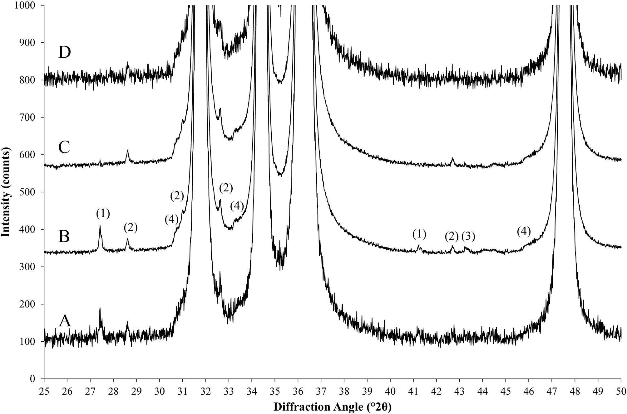
Figure 1. Processing steps of a nearly pure zincite reference sample. (a) Standard scan and (b) a high signal-to-noise (HSN) scan measured with 20 times longer counting time, followed by rescaling the intensities by a factor 1/20. (c) Scan b after stripping of impurities and rescaling. (d) Scan c with added synthetic noise pattern. Artifacts exposed in scan b: (1) rutile impurities, (2) zincite Kβ peaks, (3) corundum impurities, and (4) zincite absorption edges.
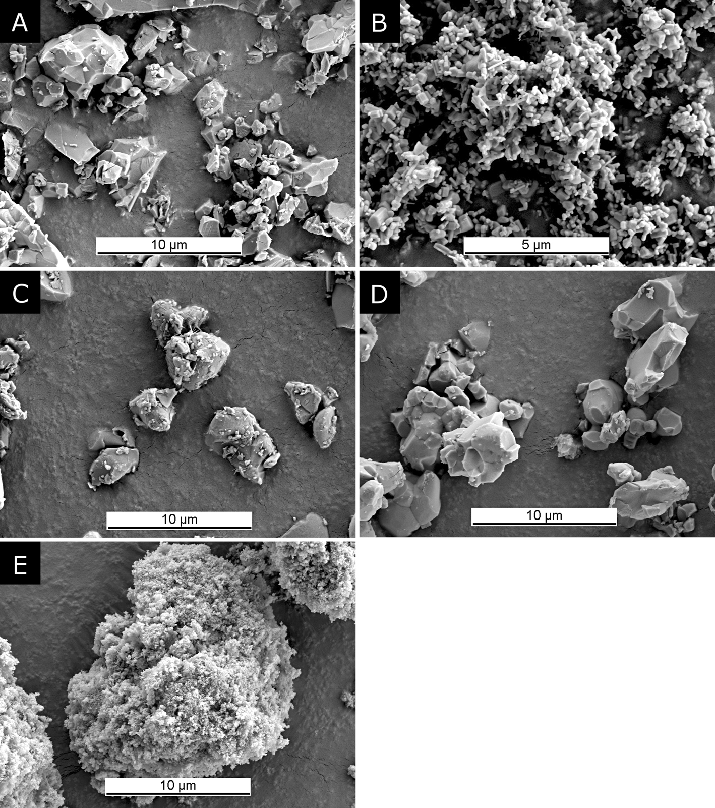
Figure 2. Scanning electron microscopy images of the materials used in examples 1 and 2 after milling for XRD sample preparation: (a) rutile, (b) zincite, (c) α-TCP, (d) β-TCP, and (e) CDHA.
For the second example simulating mixtures of three different calcium phosphate phases, we produced α-TCP Ca3(PO4)2 by heating a mixture of CaCO3 (Merck, Germany) and CaHPO4 (GFS, USA) to 1350 °C for 4 h, followed by quenching in air. Ca-deficient hydroxyapatite (CDHA; Ca9(HPO4)(PO4)OH) was obtained commercially (ACP 1.5:1, Plasma Biotal Ltd, UK) and used without thermal conditioning. β-TCP Ca3(PO4)2 was produced by heating the CDHA material to 1000 °C for 15 h. α- and β-TCP were milled for 5 min in isopropanol using the McCrone Micronizing Mill prior to the preparation of the XRD reference samples. Scanning electron micrographs of the particles after milling are shown in Figures 2(c)–2(e).
XRD data were collected on a Bruker D8 Advance diffractometer (Bruker AXS, Germany), using Ni- and digitally filtered CuKα radiation. An angular range from 8 to 120° 2θ was scanned with a step size of 0.0122°. Since the counting time of the standard method to be validated was 0.15 s/step, the reference datasets were measured with a counting time of 3 s/step, which improved the signal-to-noise ratio by factor 4.47  $\lpar = \sqrt {20} \rpar$. The intensities were then scaled back by factor 20 to obtain peak intensities identical to the standard measurement conditions. All intensity manipulations, pattern compositions, and Rietveld refinements were performed in Profex version 4.1-beta (Doebelin and Kleeberg, Reference Döbelin and Kleeberg2015). The individual steps for dataset manipulations and pattern composition are described in detail in the following sections.
B. Data manipulation
1. Reference data acquisition
XRD datasets of the nearly pure reference materials must be measured with the instrument settings to be validated but with the following exceptions: (i) the signal-to-noise ratio must be improved while maintaining the same peak intensity as the standard instrument settings and (ii) it is recommended to measure a wide angular range, e.g., up to 120° 2θ. Improved signal-to-noise ratio at constant peak intensity (HSN) can be obtained either by using a longer counting time per step and rescaling the intensities after the measurement or by averaging several datasets measured with the standard counting time. Both approaches result in the same improvement of signal-to-noise ratio by factor  $\sqrt n$ (Hassan and Anwar, Reference Hassan and Anwar2010), but if a prolonged counting time bears the risk of exceeding the detector's linear response range, merging multiple datasets measured with the standard counting time is to be preferred. If a counting time n times longer than standard conditions was used, each measured intensity value Im is rescaled as follows after the measurement:
 $$I = \displaystyle{{I_m} \over n}$$
If n repetitions were measured with standard counting time, the average intensity is calculated as follows:
 $$I = \displaystyle{{\sum\nolimits_{i = 1}^n {I_{mi}} } \over n}$$
The suppressed counting noise amplitude exposes contaminations below the detection limit of the standard measurement conditions [Figure 1, scans (a) and (b)] and allows adding realistic synthetic noise after composition of the multi-phase patterns.
2. Rietveld refinement
In a next step, the HSN scans of all reference materials are processed with Rietveld refinement. At this point, a hand-optimized highly accurate refinement strategy should be employed, independent of the standard refinement strategy to be validated. The refinement must provide accurate fits of the background and all contamination peaks (Figure 3), as well as highly precise scale factors and mass absorption coefficients (MACs) of the reference phases. If the main phase is not chemically pure, additional information from chemical analysis (e.g., XRF or ICP) should be used to improve the structure model.
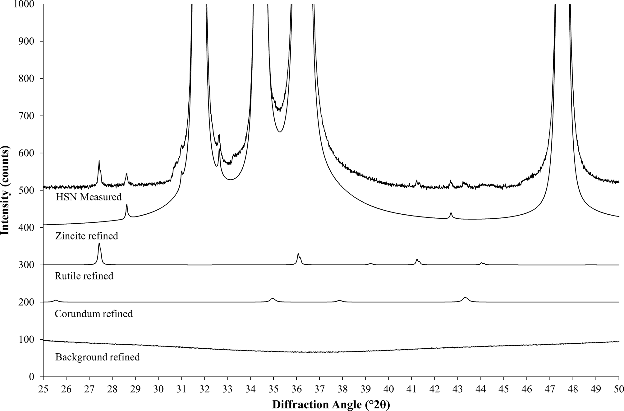
Figure 3. Rietveld refinement fits individual patterns for all phases and for the background to the measured data (stacked representation). The background was refined as a combination of a measured background and a polynomial function. The measured contribution shows tails of diffuse bumps at both sides of the displayed range, which are generated by the polymer sample holder.
As a result of the Rietveld refinement, we also obtain the following parameters of each reference phase:
-
S: Rietveld scale factor,
-
Z: number of formula units per unit cell,
-
M: mass of the formula unit,
-
V: unit cell volume,
-
μ*: MAC.
It can be easily demonstrated (see, e.g., Madsen and Scarlett, Reference Madsen, Scarlett, Dinnebier and Billinge2008) that the absolute weight fraction of phase A in a powder sample is calculated as
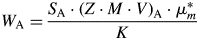 $$W_{\rm A} = \displaystyle{{S_{\rm A}\cdot {\lpar {Z\cdot M\cdot V} \rpar }_{\rm A}\cdot \mu _m^\ast } \over K}$$
where K is an instrument dependent scaling factor which is used to put W A on an absolute basis, and  $\mu _m^\ast$ is the specimen's MAC (O'Connor and Raven, Reference O'Connor and Raven1988; Madsen and Scarlett, Reference Madsen, Scarlett, Dinnebier and Billinge2008). The parameter K is usually unknown, and hence so is the absolute weight fraction W A. But, as K only depends on the instrument setup, it can be calculated from Eq. (3) in case of a single-phase reference sample containing phase R, so that W R = 1 and
  $\mu _m^\ast{ = } \mu _{\rm R}^\ast$, as follows
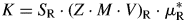 $$K = S_{\rm R}\cdot \lpar {Z\cdot M\cdot V} \rpar _{\rm R}\cdot \mu _{\rm R}^\ast $$
Determining K from a CRM and substituting it in Eq. (3) to compute absolute phase quantities of multi-phase samples is well-known as the external standard method (Jansen et al., Reference Jansen, Goetz-Neunhoeffer, Stabler and Neubauer2011a). K should not be confused with the Reference Intensity Ratio (RIR), for which the designation K is also occasionally used (Hubbard et al., Reference Hubbard, Evans and Smith1976; Hubbard and Snyder, Reference Hubbard and Snyder1988). RIR expresses the ratio of the peak intensity of an analyte to the peak intensity of a reference phase under given measurement conditions and is, therefore, phase dependent. The K value from Eq. (4), on the other hand, is independent of the phase and only instrument related. In multi-phase samples measured under identical instrument conditions and provided that no amorphous phases are present, K can be computed according to Eqs. (5) and (6) and should result in precisely the same value as obtained from the CRM in Eq. (4).
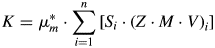 $$K = \mu _m^{\rm \ast } \cdot \sum\limits_{i = 1}^n {\lsqb S_i\cdot {\lpar Z\cdot M\cdot V\rpar }_i\rsqb } $$
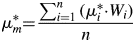 $$\mu _m^\ast{ = } \displaystyle{{\sum\nolimits_{i = 1}^n {\lpar \mu _i^\ast{\cdot} W_i\rpar } } \over n}$$
 $\mu _m^{\rm \ast }$ is the sample's bulk MAC,
  $\mu _i^\ast$ is the MAC of phase i, and Wi is the phase quantity of phase i.
We performed the calculation of K for our reference substances zincite and rutile, and compared them with the value obtained from the NIST SRM676a sample. As shown in Table I, the zincite and rutile reference samples resulted in K values lower than NIST SRM676a, indicating the presence of undetected constituents in the two reference phases.
TABLE I. Instrumental scale factors K calculated for all reference samples used in example 1.
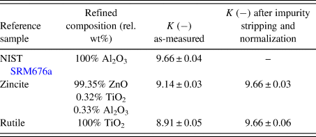
Errors represent estimated standard deviations calculated by the refinement software. In case of zincite, the value “K as-measured” represents the sum of K ZnO + K TiO2 + K Al2O3.
3. Stripping of contamination signals and normalizing for K
Now, the HSN datasets are processed to remove all contamination signals and rescaled to the target K value determined from the NIST SRM sample. Since only the diffraction signal of the reference phase I diff must be rescaled, but not the background intensity, the refined background I bkgr is subtracted from the measured intensities I obs:
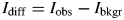 $$I_{{\rm diff}} = I_{{\rm obs}}-I_{{\rm bkgr}}$$
Then, the refined phase contributions of all contaminations obtained from the Rietveld refinement (Figure 3) are subtracted from the diffracted intensity (assuming that phase 1 is the reference phase, and phases 2 to n are contaminations):
 $$I_{{\rm pure}} = I_{{\rm diff}}-\sum\limits_{i = 2}^n {I_i} $$
Next, the K value of the pure reference phase is calculated from the Rietveld refinement, with “pure” referring to the phases zincite and rutile, respectively:
 $$K_{{\rm pure}} = S_{{\rm pure}}\cdot \lpar {Z\cdot M\cdot V} \rpar _{{\rm pure}}\cdot \mu _{{\rm pure}}^\ast $$
If K pure is lower than K SRM obtained from the CRM (NIST SRM 676a), the diffracted intensities of the reference phase are normalized:
 $$I_{{\rm norm}} = I_{{\rm pure}}\cdot \displaystyle{{K_{{\rm SRM}}} \over {K_{{\rm pure}}}}$$
The intensity of the diffraction signal I pure is now increased to the intensity that a true measurement of a single-phase sample of the reference phase would yield (I norm). Now the background intensity is added, which was not affected by the normalization:
 $$I_{{\rm ref}} = I_{{\rm norm}} + I_{{\rm bkgr}}$$
As a result, I ref represents a diffraction pattern of the reference phase based on measured intensities, that was (i) stripped of the diffraction signal of impurity phases and (ii) rescaled to the intensity the pure reference phase would yield on the same instrument configuration in absence of crystalline and amorphous impurities. When refined by Rietveld refinement, its K value according to Eq. (4) is identical to K SRM of the certified reference sample. An example of the stripped and rescaled zincite HSN dataset is shown in Figure 1, scan c. It is recommended not to strip any imperfections originating from the reference phase (Kα 3, Kβ, W Lα peaks, absorption edge), for example, by the methods proposed by Ida et al. (Reference Ida, Ono, Hattan, Yoshida, Takatsu and Nomura2018), unless the stripping is also applied to datasets of phase mixtures analyzed with the validated method later on. The reference datasets should contain all imperfections expected to occur in sample datasets to allow for a realistic determination of validation parameters.
4. Simulating multi-phase patterns
At this stage, all processed datasets of the reference substances are phase-pure, normalized to the K SRM value of a fully crystalline sample, and nearly noise free due to the initial HSN intensity manipulation. The following procedure describes how these datasets can be combined to represent mixtures of precisely known phase quantities.
The relationship between absolute phase quantity and the intensity of a phase's signal contribution is (with the exception of polymorphs) not linear. It was, however, shown by Hill (Reference Hill1991) that the intensity is directly proportional to the Rietveld scale factor S. By rearranging Eq. (3), we can determine the scale factor of phase A (S A) in any sample of known composition and K:
 $$S_{\rm A} = \displaystyle{{W_{\rm A}\cdot K} \over {{\lpar {Z\cdot M\cdot V} \rpar }_{\rm A}\cdot \mu _m^\ast }}$$
 In the special case of a phase-pure reference pattern of phase A, the scale factor  $S_{{\rm A}_{{\rm ref}}}$ becomes:
 $$S_{{\rm A}_{{\rm ref}}} = \displaystyle{{1\cdot K} \over {{\lpar {Z\cdot M\cdot V} \rpar }_{\rm A}\cdot \mu _{\rm A}^\ast }}$$
 In order to scale the intensity of reference pattern A ( $I_{{\rm A}_{{\rm ref}}\;}$) to a weight fraction W A < 1 in a multi-phase sample, it must be multiplied with the relative scale factor:
 $$I_{\rm A} = I_{{\rm A}_{{\rm ref}}\;}\cdot \displaystyle{{S_{\rm A}} \over {S_{{\rm A}_{{\rm ref}}}}}$$
 Substituting Eq. (12) for S A and Eq. (13) for  $S_{{\rm A}_{{\rm ref}}}$ results in:
 $$I_{\rm A} = I_{{\rm A}_{{\rm ref}}\;}\cdot \displaystyle{{W_{\rm A}\cdot \mu _{\rm A}^\ast } \over {\mu _m^\ast }}$$
where  $\mu _m^\ast$ is calculated according to Eq. (6) for the target phase composition. The final simulated diffraction pattern is obtained by summing all rescaled intensities of phases A to n:
 $$I_{{\rm sum}} = I_{\rm A} + I_{\rm B} + \cdots + I_n$$
and by applying a synthetic noise pattern for the intensity I sum:
 $$I_{{\rm sim}} = I_{{\rm sum}} + p\left({\sqrt {I_{{\rm sum}}} } \right)$$
p(x) generates a random Poisson-distributed number for x counts. The phase composition of the semi-synthetic diffraction pattern I sim is precisely known from the W values selected for each phase in Eq. (15). Scan d in Figure 1 shows the effect of adding synthetic noise to scan c using the function “std::poisson_distribution<int>” of the GNU libstdc++ library.
C. Application
1. Example 1: zincite and rutile
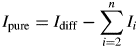
As a first example to demonstrate the procedure described above, a simple binary system of the highly symmetric phases rutile (TiO2) and zincite (ZnO) was selected. The peaks of both phases were well separated, which allowed tracking the impurity stripping and dataset synthesis process visually. HSN datasets of both reference phases covering a range of 8–120° 2θ were refined to determine their initial phase composition and K value (Table I). Traces of rutile (TiO2) and corundum (Al2O3) impurities were found in the zincite sample, but no crystalline impurities were observed in the rutile sample. The zincite dataset was then stripped of its impurity signals, and both datasets were then normalized to the reference K SRM value determined with a certified Al2O3 reference material (SRM 676a; Table I). Patterns of biphasic compositions were then created by combining the processed reference patterns and by applying synthetic counting noise as described above. The compositions and examples of the patterns are presented in Figure 4. Each composition was simulated 10 times, resulting in 210 datasets created from two reference datasets. To determine the phase composition using Rietveld refinement, the datasets were processed with Profex by the BGMN Rietveld kernel version 4.2.23 (Doebelin and Kleeberg, Reference Döbelin and Kleeberg2015) using three different refinement strategies. The parameters refined in all three strategies are listed in Table II. Strategy “no restrictions” provided the best possible profile if both phase patterns were well defined, i.e., their intensities were high enough that the peak shapes were not obstructed by the noise pattern. Strategies “restricted zincite” and “restricted rutile” used the same elaborate refinement for one phase, but refined only basic profile parameters of the second phase. All 210 datasets were refined with the three strategies in a batch without user interaction. The resulting phase quantities were analyzed statistically (Table III). Figure 5 presents the difference between the refined zincite quantity and the nominal (simulated) value in the range of low rutile content (<10 wt%), major content of both phases (10–90 wt%), and low zincite content (<10 wt%). Due to the normalization to 100 wt%, rutile quantities W rutile correspond to 100 – W zincite.
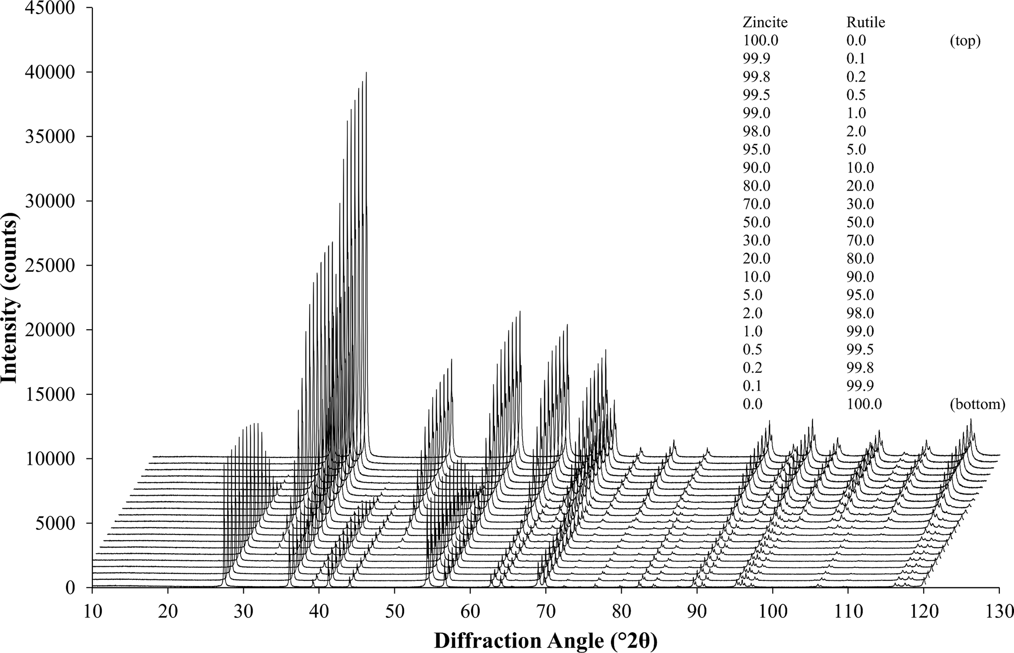
Figure 4. 21 diffraction patterns of different composition created from the stripped and normalized zincite and rutile reference patterns. The patterns represent I sim [Eq. (17)], including the background signal and synthetic counting noise. Each composition was simulated and refined 10-fold, resulting in 210 multi-phase datasets created from two reference datasets. The legend shows the simulated phase composition in wt%.
Figure 5. Differences between refined and nominal zincite quantities obtained from three different refinement strategies. The x-axis is split into three segments to enhance the visibility of the data points close to 0 and 100 wt% zincite. The strategy optimized for the displayed compositional range is shown in red. Error bars represent standard deviations (n = 10).
TABLE II. Structural parameters refined in the three refinement strategies of example 1.

(T), Texture; (MS), Micro-strain; (ACS), Anisotropic crystallite sizes; (3CS), Trimodal crystallite size distribution; (TDS), Common thermal displacement parameters. The following parameters were refined in all strategies: background polynomial coefficients, sample height displacement, and unit cell dimensions, scale factors, and isotropic peak broadening of both crystalline phases.
2. Example 2: calcium phosphate cement
The second example was based on a reaction commonly used in ceramic bone cements. The metastable high-temperature phase α-TCP undergoes a hydration reaction when mixed with water to form nano-crystalline CDHA. α-TCP often contains contaminations of β-TCP, a polymorph that is non-reactive in water and stable at room temperature. Monitoring the cement reaction progress by XRD thus involves the quantification of variable contents of highly crystalline α-TCP and nano-crystalline CDHA, and a constant amount of β-TCP. The reference materials used in this example were measured with a 20-fold longer counting time per step than standard settings and then processed with Rietveld refinement to quantify impurity phases and to determine the initial K values (Table IV). Afterwards, impurity signals were stripped, and the datasets were normalized to a common K value. However, instead of using a K SRM value obtained from the certified Al2O3 sample, the value determined for the α-TCP sample was used as a reference. The resulting normalized datasets prior to multi-phase pattern simulation are shown in Figure 6. K values were lower than in the first example due to instrumental fluctuations that occurred during a gap of several weeks between the data collections of the two examples. Since the K value is directly related to the intensity of the primary beam, a gradual decrease over time is an expected symptom of an aging X-ray tube. Multi-phase patterns with added counting noise were created 10-fold for each simulated composition. The simulated β-TCP content was kept constant at 10 wt%, whereas α-TCP and CDHA contents were varied from 90 to 0 wt% α-TCP, and 0 to 90 wt% CDHA, respectively. This represented the complete cement reaction in presence of a constant amount of β-TCP contamination. The simulated datasets were refined using the strategy shown in Table V . Refined phase quantities are shown in Table VI, a statistical analysis is presented in Table VII, and an example refinement is shown in Figure 7.
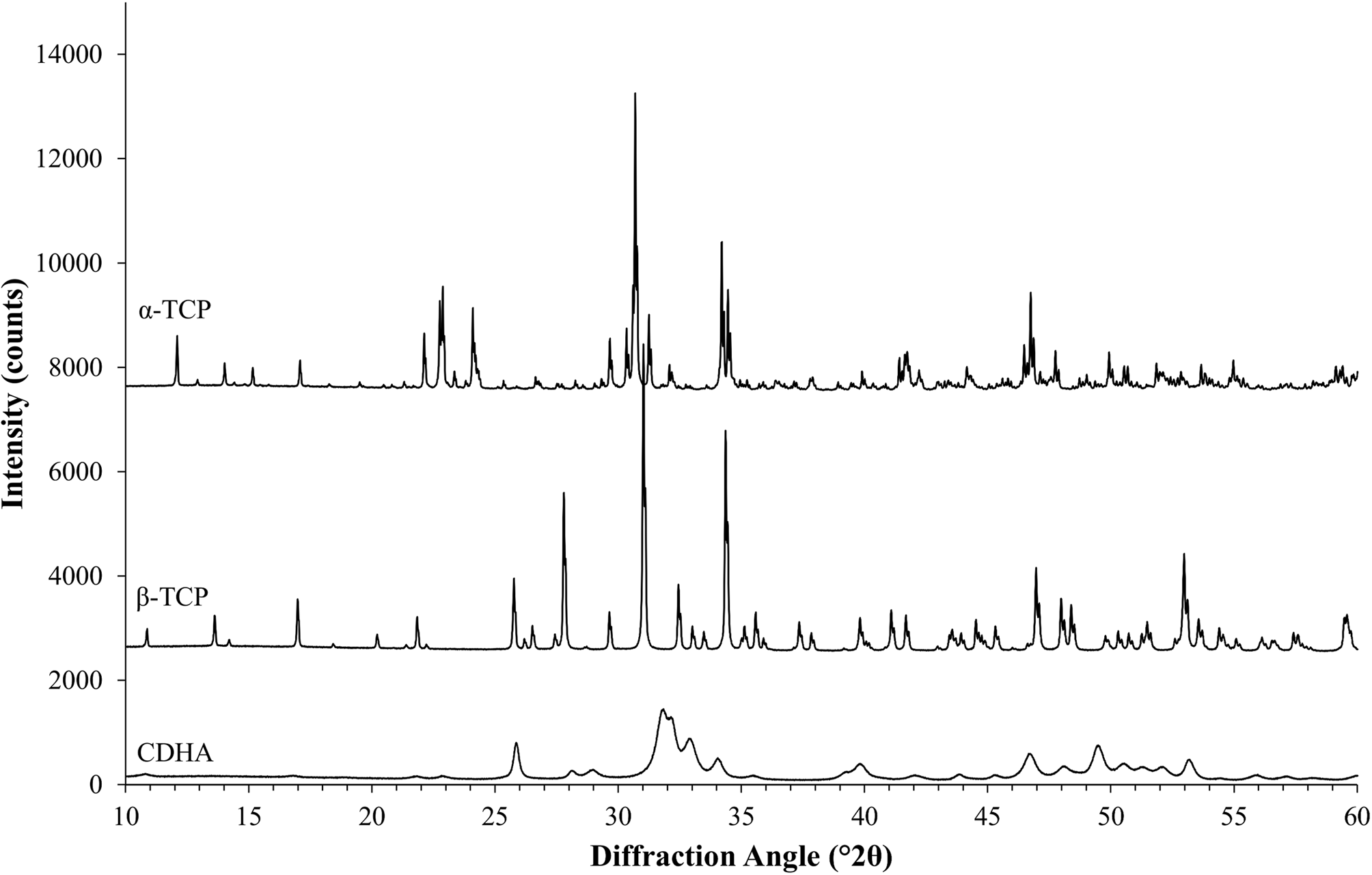
Figure 6. The measured HSN reference patterns of α-TCP, β-TCP, and CDHA after stripping of impurities and normalization to a common K factor show several regions of peak overlap among α-TCP and β-TCP, as well as among β-TCP and nano-crystalline CDHA.
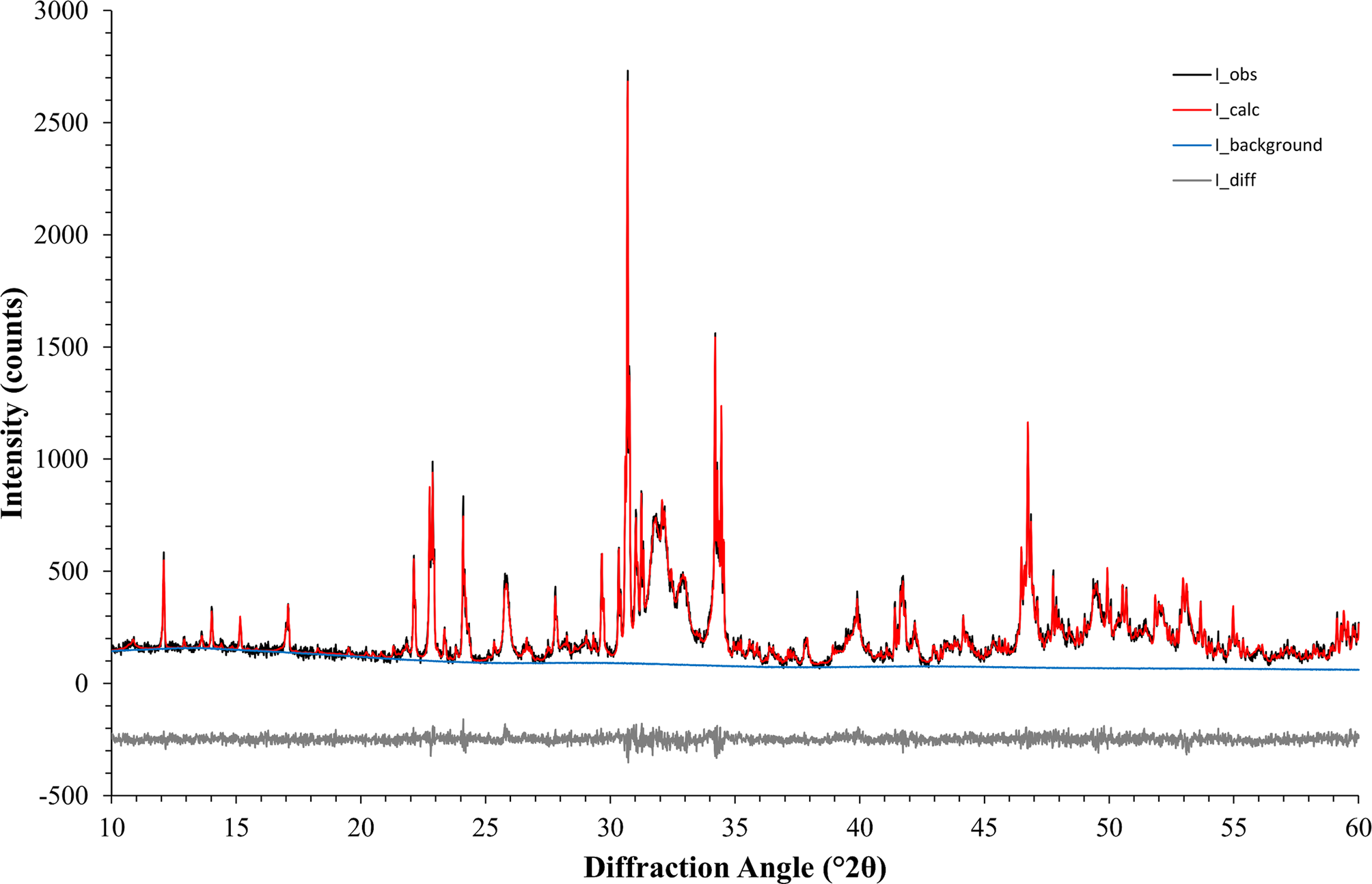
Figure 7. An example refinement of example 2 (nominal composition 45 wt% α-TCP + 45 wt% CDHA + 10 wt% β-TCP) converged with χ 2 = 1.20.
TABLE IV. Instrumental scale factors K calculated for all reference samples used in example 2.
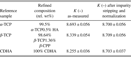
Errors represent estimated standard deviations calculated by the refinement software.
β-CPP: β-Ca pyrophosphate (Ca2P2O7).
TABLE V. Structural parameters refined in example 2.
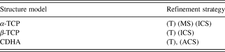
(T), Texture; (MS), Micro-strain; (ICS), Isotropic crystallite size; (ACS), Anisotropic crystallite sizes. The following parameters were refined in all strategies: background polynomial coefficients, sample height displacement, and unit cell dimensions, scale factors.
TABLE III. Validated parameters for zincite and rutile using three different refinement strategies.
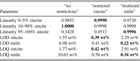
Values in their optimized compositional range are shown in bold typeset.
LOD = limit of detection = x blank + 3⋅SD
LOQ = limit of quantification = xblank + 5⋅SD
TABLE VI. Refinement results of example 2 containing α-TCP, CDHA, and β-TCP.
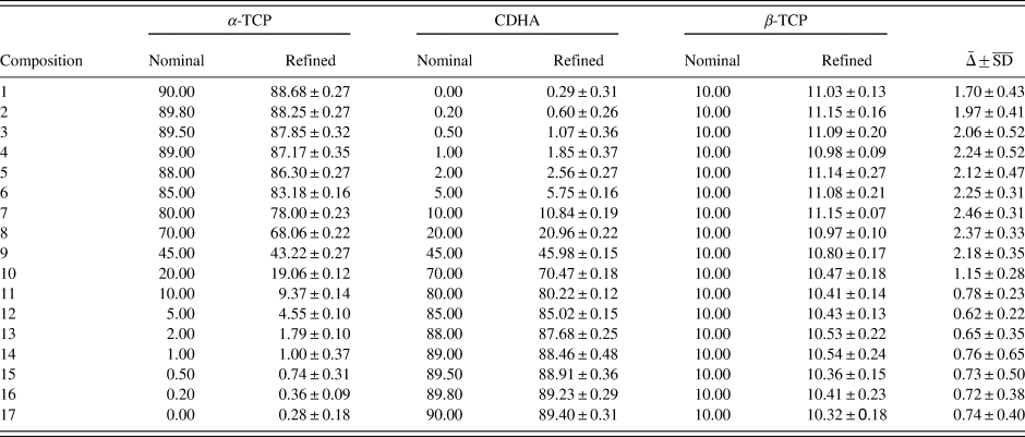
All values are given in wt%, errors represent one standard deviation (SD, n = 10). A quality index  $\bar{{\rm \Delta }}$ was calculated as
  $\bar{{\rm \Delta }} = \sqrt {{\rm \Delta }_{\alpha -{\rm TCP}}^2 + {\rm \Delta }_{{\rm CDHA}}^2 + {\rm \Delta }_{\beta -{\rm TCP}}^2 }$, where Δ = Nominal – Refined.
  $\overline {{\rm S}{\rm D}} = \sqrt {{\rm S}{\rm D}_{\alpha -{\rm TCP}}^2 + {\rm S}{\rm D}_{{\rm CDHA}}^2 + {\rm S}{\rm D}_{\beta -{\rm TCP}}^2 \;}$.
TABLE VII. Validated parameters for α-TCP and CDHA in a mixture containing 10 wt% β-TCP contamination.
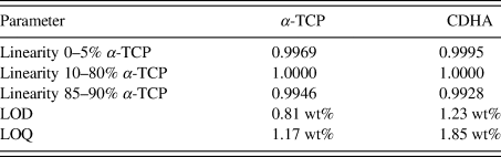
LOD = limit of detection = x blank + 3⋅SD
LOQ = limit of quantification = x blank + 5⋅SD.
To assess the effect of the number of simulations on the statistical analysis, the composition 45 wt% α-TCP + 45 wt% CDHA + 10 wt% β-TCP of example 2 was again simulated and refined 100 times. The cumulative moving average  $\bar{Q}_{1 \ldots n}$, the standard deviation, and the standard error were calculated for the first n datasets, where n was increased from 1 to 100 (Figure 8).
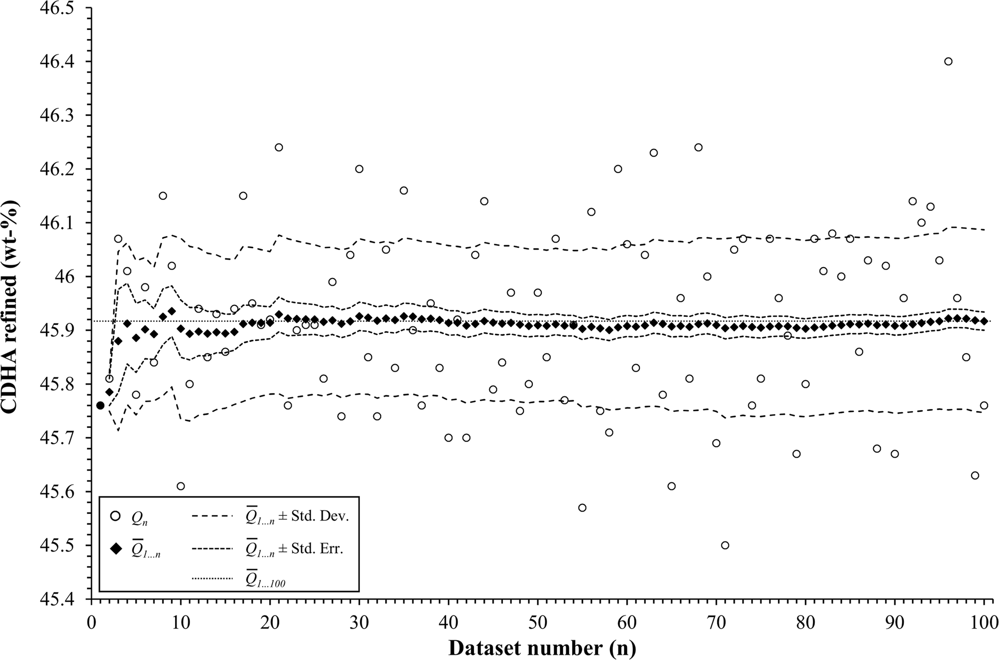
Figure 8. The mean value  $\lpar \bar{Q}\rpar$ and standard deviation (Std. Dev.) of the refined α-TCP phase quantity in example 2 fluctuated at low numbers of simulations, but stabilized when at least 29 datasets were processed. Between 29 and 99 repetitions, the mean value
  $\bar{Q}_{1 \ldots n}$ remained within one standard error (Std. Err.) from the mean value of 100 repetitions
  $\lpar \bar{Q}_{1 \ldots 100}\rpar$.
III. RESULTS AND DISCUSSION
Phase quantification by XRD analysis is particularly challenging to validate not only because the availability of CRMs is extremely limited and in most cases not suited to replicate a particular phase system of interest but also because the results are highly susceptible to matrix effects. The detection limit of phase A in mixture with phase B is different than in mixture with phase C if the amount of peak overlap with phases B and C is different. Therefore, a validation must be targeted precisely at the composition of the samples to be measured, and for compositions of more than two phases, taking into account all possible phase combinations can easily lead to enormous numbers of compositions. As a consequence, the literature on XRD method validation is relatively scarce and mostly focuses on simple binary phase systems. Siddiqui et al. (Reference Siddiqui, Rahman, Korang-Yeboah and Khan2015) validated the quantification of warfarin sodium products in two different matrices. The determination of accuracy, precision, linearity, limits of detection and quantification, and robustness was carried out using three concentrations measured six times, and three concentrations measured once. The effect of the instrument setup and Rietveld refinement strategy on the quantification of Tibolone Form I and Form II was assessed by Silva et al. (Reference Silva, Ambrósio, Epprecht, Avillez, Achete, Kuznetsov and Visentin2016), who demonstrated that matching the refinement strategy to the expected phase composition improved accuracy and precision of the refinement. While both studies validated phase quantification in manageable binary phase systems, Eckardt et al. (Reference Eckardt, Krupicka and Hofmeister2012) used a variety of different materials, including certified standards for soil and Portland cement clinker, to perform a comprehensive validation fulfilling the requirements of ISO/IEC 17025. The study included a proficiency test comparing the performance of 13 laboratories determining the composition of three mixtures of ceramic, metallic, and organic components. Interlaboratory studies such as the proficiency study published by Eckardt et al. (Reference Eckardt, Krupicka and Hofmeister2012) for forensic materials, by Stutzman (Reference Stutzman2005) for hydraulic cements, by Döbelin (Reference Döbelin2015) for bioceramics, those organized by the International Union of Crystallography (Madsen et al., Reference Madsen, Scarlett, Cranswick and Lwin2001; Scarlett et al., Reference Scarlett, Madsen, Cranswick, Lwin, Groleau, Stephenson, Aylmore and Agron-Olshina2002), or competitions such as the Reynolds cup organized by the Clay Minerals Society are often used to compare the performance of laboratories. They cannot be considered as a viable alternative to a full method validation, but they provide supporting information and their participation is encouraged in ISO/IEC 17025.
The procedure for the numerical manipulation of reference datasets we present here facilitates the validation of XRD phase quantifications in situations where phase-pure and fully crystalline reference materials are not available, and in systems with a large number of phases whose number of possible combinations cannot be produced economically. We demonstrated that small diffraction signals of impurities can be subtracted from HSN diffraction patterns of nearly pure reference materials (Figure 1), and the residual artifacts are masked by counting noise. The artifacts depend on the quality with which the Rietveld refinement fits the impurity signals (Figure 3). Although the procedure is in theory capable of removing any number and intensity of impurity signals, artifacts from the subtraction of strong signals may exceed the counting noise and thus leave artifacts in the final composed multi-phase patterns. It is, therefore, recommended to limit the use of this approach to reference materials of high initial purity. The peak profiles modeled by the Rietveld algorithm are only used to subtract contamination signals. The peak shape of the reference phase remains unaffected. This is an important distinction from datasets simulated by the Rietveld algorithm. Any peak computed by the algorithm's profile function can be fitted with the same algorithm with perfect accuracy. Using synthetic datasets simulated with the Rietveld software as input files for the refinement thus results in unrealistically high precision and accuracy, even in the presence of counting noise. The process we propose for stripping impurity signals and rescaling the reference peaks, on the other hand, preserves the peak shape of the measured datasets, including all technical imperfections such as the absorption edge, satellite peaks, and potential distortions originating from instrument misalignment [Figure 1, scan (c)]. In addition to reducing the efforts for sample preparation to a manageable level, combining reference datasets mathematically also avoids problems potentially arising from blending powder components. Intense homogenization may introduce changes in microstructure and crystallinity or reactions among the phases, which would result in a putative systematic error when comparing refined with nominal phase quantities. The nominal phase content of mathematically combined datasets, on the other hand, is precisely known.
Optimum instrument settings for standard data acquisitions may be limited by economic considerations. If measurement time per sample is limited, the choice of counting time per step and angular range should be matched to the purpose of the analysis. For example, if the purpose is to demonstrate phase purity, the limits of detection and quantification benefit from a longer counting time over a limited angular range resulting in an improved signal-to-noise ratio. On the other hand, if the quantification of main phases and the determination of their crystallographic parameters (cell parameters, distinction of crystallite size and micro-strain, atomic site parameter including site occupancy factors and thermal displacement parameters) are the primary goal of the analysis, the results may benefit from a wider angular range measured with a shorter counting time. As discussed previously, the HSN datasets of pure reference materials used as input files for dataset synthesis must expose features below the noise level of standard measurements. Their signal-to-noise ratio must, therefore, be suppressed either by merging multiple datasets or by rescaling a dataset measured with longer counting time. In addition, correct determination of the instrumental factor K requires accurate refinement of potential substitutions and thermal displacement parameters. The HSN datasets should, therefore, not only focus on maximum signal-to-noise ratio but also cover an extended angular range allowing stable refinement of angular-dependent crystallographic parameters.
In our first example, we processed two reference datasets of rutile and zincite to eliminate impurity signals and to normalize the intensities of the main phases to a given instrumental K SRM value. As shown in Table I, the K values prior to normalization of both samples were slightly below the value obtained from the certified Al2O3 reference. If all constituents of the samples were crystalline and refined correctly, identical K values for all three reference samples would have been expected. Lower K values indicate the presence of (i) amorphous constituents, (ii) undetected crystalline phases, or (iii) undetected chemical substitutions resulting in a wrong estimate of the molecular mass of the unit cell content. We excluded chemical substitutions by using raw materials of very high purity, and the detection limits were too low for undetected crystalline phases to cause a reduction of K in the observed extent. The most likely explanation for lower K values is, therefore, the presence of amorphous phases or domains. This example also demonstrates that physical mixtures of the two apparently phase-pure materials NIST SRM 676a and rutile would not represent the assumed ratio of crystalline corundum and rutile because undetected amorphous constituents would be introduced with the rutile material. Such physical mixtures would, therefore, be unsuitable for a method validation due to the unknown true nominal ratio of the crystalline phases. After stripping the impurity signals from the zincite dataset and normalizing the zincite and rutile intensities to the reference K SRM value, refinement of the processed datasets resulted in identical K values (Table I).
From the normalized zincite and rutile reference patterns, we created 21 different compositions in 10-fold replication (Figure 4), resulting in 210 datasets in total. Since the reference patterns were rescaled and numerically merged but their measured peak shape and background evolution were preserved, we refer to the multi-phase patterns as “semi-synthetic” datasets. Refining them with three different refinement strategies exposed the strengths and weaknesses of each strategy in terms of accuracy and precision of the refined phase quantities. The “no restrictions” strategy refined a large number of profile parameters for both phases. It yielded by far the most accurate results at a 50:50 wt% phase ratio (Figure 5), albeit with a greater standard deviation than the more restricted strategies. At lower and higher zincite content, it tended to over-estimate the less abundant phase, and when the rutile content reached 1 wt% or less, the refinement became unstable. The strategies restricting refinement of one of the two phases to basic profile parameters clearly showed that the quantification was more stable (higher accuracy and precision) when the restricted phase approached 0 wt%.
A more demanding composition of three phases, including one with overlapping peaks and severe crystallite size-related peak broadening, was chosen as a second example. The 17 mixtures of α-TCP, CDHA, and β-TCP were simulated 10-fold and refined with a strategy of moderate complexity (Table IV). Figure 7 shows an example refinement of composition 45 wt% α-TCP + 45 wt% CDHA + 10 wt% β-TCP that demonstrates the complexity of the overlapping phase signals. The mean refined phase quantities (Table VI) showed that α-TCP was slightly under-estimated for the most part of the compositional range, but became over-estimated at a nominal quantity below 1.0 wt%, when the peak height approached the counting noise amplitude. The constant amount of β-TCP impurity was over-estimated in all compositions. Validation parameters (Table VII) showed excellent linearity of both α-TCP and CDHA phase quantities in the entire simulated compositional range, but relatively high limits of detection and quantification due to over-estimation at low phase content. If an implementation of this quantification method required lower limits, a refinement strategy optimized for low phase content, possibly combined with a slower counting time to improve the signal-to-noise ratio, could be considered.
According to the “Guide to the expression of uncertainty in measurement” (JCGM, 2008), the number of repetitions n from which an arithmetic mean value and experimental standard deviation are determined, should be large enough to ensure that both values are reliable estimates of the population. In other words, the number of simulations n for each phase composition must be sufficiently large to reliably represent the mean values and standard deviations obtained from an infinite number of measurements of a real sample. To assess how the refined mean phase quantities  $\lpar \bar{Q}\rpar$, their experimental standard deviation (Std. Dev.), and standard error of the mean
  $\lpar {\rm Std}.\,{\rm Err}. = {\rm Std}.\,{\rm Dev}./\sqrt n \rpar$ are affected by the number of repetitions n, we simulated one composition of example 2 (45 wt% α-TCP + 45 wt% CDHA + 10 wt% β-TCP) 100 times. The statistical parameters were then determined for the first n datasets, while n was gradually increased from 1 to 100. The arithmetic mean of the refined α-TCP phase quantity, as well as the experimental standard deviation and standard error of the mean for n ranging from 1 to 100 are presented in Figure 8. The mean and standard deviation were strongly affected by individual results when n was less than 29. For n ≥ 29, both values approached the mean and standard deviation obtained from 100 repetitions. Less fluctuation was observed among the mean values of refined CDHA phase quantities (not shown), but the standard deviations approached the values obtained from 100 repetitions when n was ≥ 20. These findings clearly show that the determination of realistic mean phase quantities and standard deviations requires a number of repetitions (29 in our example 2) which in most cases can no longer be economically justified with real samples. The number of simulated semi-synthetic datasets can, however, be increased without significant effort. Especially in combination with a refinement software that supports batch processing, the additional effort due to a high number of repetitions only manifests itself in an increased computing effort, which is of negligible economic impact.
Using only one processed reference dataset per phase to create all semi-synthetic multi-phase datasets was sufficient to assess the effect of the refinement strategy on the quality of the results. However, a validation also requires operator, instrumental, and environmental influences on the results to be quantified. These factors can be taken into consideration by preparing and measuring a larger number of HSN datasets for each reference material by multiple operators on different days, which are then selected in a random manner to compose the multi-phase datasets. Six reference datasets of two (three) materials can be combined in 36 (216) unique pairs, thus minimizing repetitions and incorporating the external error sources in the semi-synthetic datasets. Using multiple reference datasets for each phase also introduces a variability of the measured background signal and the refined background polynomial, which is subtracted from the measured intensities [Eq. (7)] prior to impurity stripping and intensity normalization. This additional source of error further improves the significance of semi-synthetic datasets approximating datasets of real phase mixtures.
The procedure we presented here produces highly realistic diffraction patterns of precisely known phase composition. In real multi-phase mixtures, however, the ratio of diffraction signal intensities of the individual phases can be biased by micro-absorption. This phenomenon occurs in samples containing phases of high absorption contrast and particles large enough to absorb a significant amount of radiation. In that case, X-rays interacting with strongly absorbing phases are diffracted by a smaller interaction volume than those interacting with phases exhibiting low absorption coefficients. As a result, the diffraction signals of weakly absorbing phases are emphasized, and those of strongly absorbing phases are suppressed, and the ratios of signal strength no longer reflect the ratio of phase abundances. The bias diminishes if the particles are small enough to allow X-rays interacting with a number of particles that is representative for the composition of the sample. The first approach to mitigating micro-absorption bias is, therefore, a reduction of particle size. Madsen and Scarlett (Reference Madsen, Scarlett, Dinnebier and Billinge2008) also proposed using a wavelength at which the absorption contrast is minimized or at which absorption is generally low, thus allowing the radiation to interact with a large sample volume. Brindley (Reference Brindley1945) proposed a mathematical correction for the effect of micro-absorption on phase quantification, but the model requires knowledge of the particle size and is severely limited by broad and skewed particle size distributions. Our procedure for the preparation of semi-synthetic datasets does not simulate the effect of micro-absorption in its current incarnation. In samples containing phases of strong absorption contrast, an additional systematic error may thus be present which is not accounted for by our approach. This additional bias can be determined experimentally by quantifying a real mixture of the reference phases. Differences in K values of the pure substances before processing of the datasets must be taken into account to determine the actual expected phase fractions. For example, a precise 50:50 mixture by weight of our rutile and zincite reference materials effectively contains 46.27 wt% rutile + 47.00 wt% zincite + 0.16 wt% corundum + 6.57 wt% unknown phases in absolute weight fractions, or 49.52 wt% rutile + 50.31 wt% zincite + 0.17 wt% corundum in relative weight fractions, according to the compositions and K values listed in Table I. If the quantification of a real mixture results in a systematic error greater than that determined from the semi-synthetic datasets, the additional bias should be attributed to micro-absorption.
A second limitation of our approach is related to preferred orientation, which tends to be over-emphasized in datasets obtained by a numerical combination of stripped and normalized reference patterns. Anisotropic crystals within a biphasic mixture may be stabilized by the crystals of the second phase, which reduces preferred orientation. The reference patterns used to compose semi-synthetic datasets, however, are measured in nearly pure condition and composed with other phase patterns numerically after data collection. They may, therefore, be devoid of the stabilizing effect of the other phases and show stronger signs of preferred orientation. Full-pattern data processing methods, including Rietveld refinement, are generally more robust against the bias emerging from orientation effects than single-peak based methods because the overall intensity of the pattern remains unchanged. Although Rietveld refinement programs implement algorithms for refinement of preferred orientation parameters, the common March–Dollase function (Dollase, Reference Dollase1986) is only a crude approximation to reality and may not adequately correct for extreme orientation effects. More sophisticated models using symmetrized spherical harmonics (Järvinen, Reference Järvinen1993) have been implemented in some programs, and the implementation in BGMN, the Rietveld refinement kernel applied in the present study, has been found to be particularly robust even in cases of strong texture (Bergmann et al., Reference Bergmann, Monecke and Kleeberg2001). The extent of systematic errors in phase quantifications introduced by preferred orientation thus not only depends on the extent of orientation but also on the correction model implemented in the refinement program. From a regulatory point of view, over-estimation of errors is generally considered less critical than under-estimation because a conservative estimate does not imply unrealistic precision and accuracy. The over-emphasis of texture in our reference datasets may lead to such an over-estimate if phases prone to severe preferred orientation are involved. Therefore, more rigorous strategies may be required to mitigate preferred orientation than would be necessary in case of multi-phase samples.
The limitations of our method discussed above clearly illustrate that compliance with the common rules for good sample preparation and data collection is of utmost importance. These rules aim at minimizing artifacts due to micro-absorption and texture as well as changes in the sample during preparation, while also achieving optimal particle statistics.
All data manipulations described in Eqs. (1)–(17) were performed with the programs Profex version 4.1-beta (Doebelin and Kleeberg, Reference Döbelin and Kleeberg2015) and BGMN version 4.2.23 (Bergmann et al., Reference Bergmann, Friedel and Kleeberg1998). Rietveld refinements, calculation of MACs, and calculations of K values [Eqs. (3)–(6)] were performed with BGMN using Profex as a graphical user interface. Algorithms for pattern merging and rescaling [Eqs. (1) and (2)], impurity stripping and normalization [Eqs. (7)–(11)], and pattern simulation [Eqs. (12)–(17)] were implemented directly in Profex and are available in versions 4.1 and newer.
IV. CONCLUSION
We present a procedure for obtaining a large number of XRD datasets with exactly known phase composition from relatively pure reference materials that can be used to validate phase quantification methods. This simplifies the search for high-purity reference substances, and a large number of compositions in a statistically significant number of replicates can be processed with little effort. Especially in systems containing more than two phases, the number of required mixing ratios can quickly become unmanageable. By using semi-synthetic datasets, the detection and quantification limits, precision, accuracy, and linearity can be reliably determined in such systems.


 Open access