Fluctuations of the Sea Level, Caused by Gravitational and Infra–Gravitational Sea Waves


V.I. Il’ichev Pacific Oceanological Institute FEB RAS, 690041 Vladivostok, Russia
*
Author to whom correspondence should be addressed.
J. Mar. Sci. Eng. 2020, 8(10), 796; https://doi.org/10.3390/jmse8100796
Submission received: 4 September 2020
/
Revised: 10 October 2020
/
Accepted: 10 October 2020
/
Published: 13 October 2020
(This article belongs to the Special Issue Sea Level Fluctuations)
Abstract
:In the article we analyzed the results of processing experimental data of the range of surface gravity sea wind waves (2–20 s) and the range of infra-gravitational sea waves (30 s–10 min), obtained on the laser meter of hydrosphere pressure variations. The laser meter of hydrosphere pressure variations was installed for a long time on the bottom at different points of the Sea of Japan shelf. This paper presents the results of the analysis of swell waves caused by the KOMPASU typhoon, which passed over the Sea of Japan on 2–3 September 2010. Several mechanisms of the generation and propagation of waves with different periods during the typhoon movement are considered. In the course of the analysis, we studied the connection between variations of the main periods of gravitational sea waves with the dispersion and the Doppler effect, variations of speed and direction of the wind in a typhoon zone. The nonlinearity of the process of wave period change caused by dispersion is estimated. In the combined analysis of variations of hydrosphere pressure in the ranges of gravitational and infra-gravitational sea waves, we studied their energy relationships and determined regional infra-gravitational sea waves, which make a significant contribution to the energy of the infra-gravitational range.
1. Introduction
Many results of the theory of sea surface wind waves can be considered the classics of hydrodynamics, the starting point of which is the Archimedes’ work “On floating bodies” [1]. In the works of Newton, Pascal, and Euler, this principle was developed, with receipt of analytical equations of hydrodynamics, which are the basis for describing sea gravity wind waves. All basic equations of hydrodynamics are inherently nonlinear; the main way to solve them was to find particular solutions for certain initial conditions. The next stage in developing the theory of waves started with the creation of a new method for solving nonlinear partial differential equations. In 1967, physicists J. Green, C. Gardner, and M. Kruskal [2], using the method of the inverse scattering problem that they created, showed that the Korteweg-de Vries equation has solutions absolutely for all initial conditions.
The same year, T. Benjamin and J. Feyer [3] by theoretical calculations managed to show that because of the instability of a periodic wave in deep water, the waves break into the groups. V.E. Zakharov obtained the equation, describing this process, in 1968. This equation describes the formation of groups of several dozen waves, while the average wave in the enveloping curve of the entire group is the largest, but if there are too many waves in the group, then this group will split into several ones. Basically, after that, theoretical studies were reduced to numerical solutions and modeling of nonlinear wave fields. In the early 1980s, there was rapid progress in experimental and numerical research, in this respect, we should mention the works of M. Longuet-Higgins [4,5,6], K. Hasselman [7,8], and E. Caponi [9].
Currently, in the world there are several most common models used to calculate and predict wind surface waves: spectral-parametric wave models of the 2nd generation AARI-PD2, discrete models of the 3rd generation—WAM, WAVEWATCH, and SWAN, which take into account nonlinear effects and are designed specifically for calculating wind waves in shallow water areas [10,11,12].
Further research developed with varying success, but many problems have not been solved yet: mainly, the problems associated with matching the obtained experimental data and the results of model-theoretical studies. We can mention some of them in this work: (1) spatiotemporal development of the wave process during nonlinear motion of sea gravity surface wind waves initiation sources (typhoons, cyclones, etc.); (2) variations in the periods of gravity waves not associated with the dispersion process; (3) role of gravity waves in the initiation of sea infragravity waves and their regional peculiarities; and (4) initiation of rogue waves and the role of gravity waves in this process. In this paper, special attention will be paid to solving the above problems, basing on obtained experimental data, the results of their processing and analysis.
2. Experimental Data
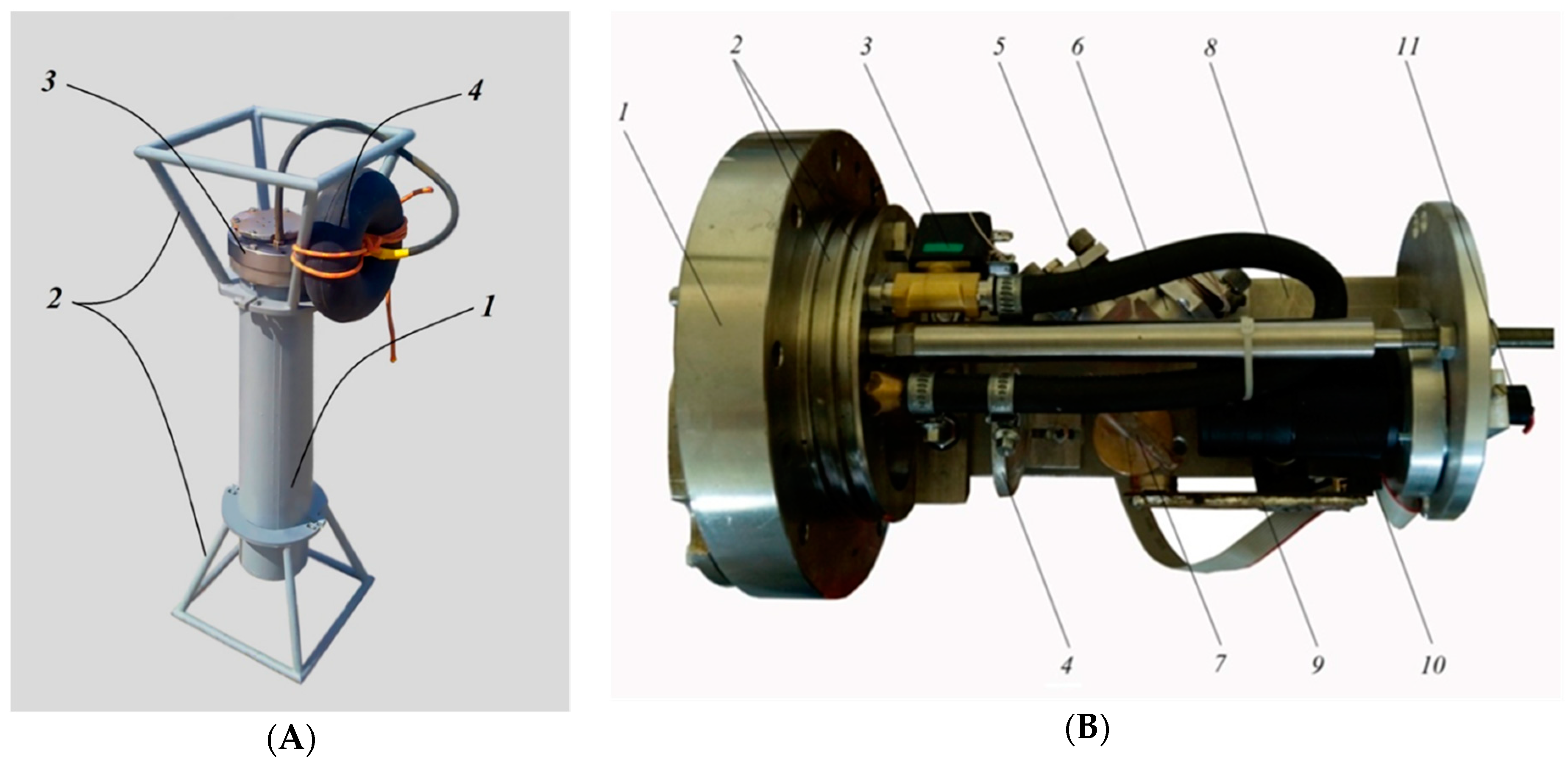
The experimental data analyzed in this paper were obtained using a laser meter of hydrosphere pressure variations, created on the basis of an equal-arm Michelson interferometer with a frequency-stabilized helium-neon laser [13]. Instruments of this type carry out measurements all year round in the permanent mode at their installation point; the registration is interrupted only for short periods of time for adjustment and troubleshooting. The appearance and optical scheme of the laser meter of hydrosphere pressure variations are shown in Figure 1.
The laser meter of hydrosphere pressure variations (Figure 1A) is a cylindrical housing (1), which is mounted in the protective grating (2). One side of the housing is hermetically sealed and has a cable port. The other side is sealed with a removable cover (3). Outside the instrument, there is an elastic air-filled container (4). Its outlet is connected with a tube to a compensation chamber, located in the removable cover. The sensitive element of the laser meter of hydrosphere pressure variations is the round membrane fixed in its removable cover in such a way that one side of it is in contact with water, and the other side faces the inside of the instrument and is a part of the Michelson interferometer.
All optical elements of the laser meter of hydrosphere pressure variations (Figure 1B) are rigidly fixed on the optical base (8). The laser beam (11) comes through the collimator (10) to the plane-parallel dividing plate (7), which splits it into two beams—measuring and reference. The first (measuring) beam is directed to the lens (4), then, through the optical window—to the mirror-coated membrane located in the cover (1). After reflecting from the membrane, the beam again comes to the lens and then to the dividing plate (7), from which it is reflected to the photodiode of the resonance amplifier (9). The second (reference) beam, after the dividing plate, passes through the system of control mirrors (5) and (6), mounted on piezoceramic bases. Then, like the measuring beam, it comes to the photodiode of the resonance amplifier. By means of these two beams, the interference pattern is adjusted; its change corresponds to the variations of hydrosphere pressure affecting the membrane.
It is designed to record hydrosphere pressure variations in the frequency range from 0 (conventionally) to 1000 Hz, with an accuracy of 0.1 mPa at sea depths of up to 500 m using a specially designed compensation chamber. The laser meter of hydrosphere pressure variations was installed on the bottom at various points of the Sea of Japan shelf and measurements were taken with a duration from several days to several months. The obtained experimental data were transferred in real time to the laboratory room located at Schultz Cape, the Sea of Japan, Primorsky Region of the Russian Federation, and, after preliminary processing, were loaded in the experimental database. Subsequently, the experimental data were processed according to the set tasks. In the low-frequency sound range (20–1000 Hz), the propagation regularities of hydroacoustic signals, generated, among other things, by low-frequency hydroacoustic emitters, were investigated [14]. In the higher frequency range (1–20 Hz), the formation peculiarities of the microseisms in the “voice of the sea” range were studied [15]. The scope of our interests in the lower frequency range included studies aimed at investigation of the free oscillations of the Sea of Japan and some of its bays, recession-setup phenomena, tidal dynamics, and the relationship of oscillations and waves of the infrasonic range of the hydrosphere with oscillations and waves of the corresponding period of the atmosphere and lithosphere. Of interest are also processes in the range of gravity sea wind waves (2–20 s), in the range of infragravity sea waves (30 s–10 min), and nonlinear effects leading to the formation of surface and internal soliton-like disturbances of large amplitude. It is these processes, described in the previous sentence, that we will pay attention to in this paper. Along with tsunamis, these processes lead to significant variations in sea level, in some cases causing serious damage to human activities.
When processing the experimental data of the gravity sea wind waves range, we found that the temporal change in the periods of wind waves, emerging from the typhoon action zone, so-called swell waves, did not occur linearly as a consequence of the dispersion law. For further analysis, 16 record fragments with a characteristic change in the period of surface waves were selected. The fragments sampling rate was 1000 Hz. When processing the data, high frequencies were filtered by the Hamming window, the filter order was 3000, the cutoff frequency was 1 Hz, followed by 1000 times decimation. Thus, the extreme frequency in the spectral analysis was 500 mHz (2 s). To get rid of the low-frequency background in the signal, low frequency filtering was also carried out by the Hamming window, the filter length was 1500, the cutoff frequency was 50 mHz (20 s). Thus, a frequency range, corresponding to periods of surface wind waves, was selected from the entire signal.
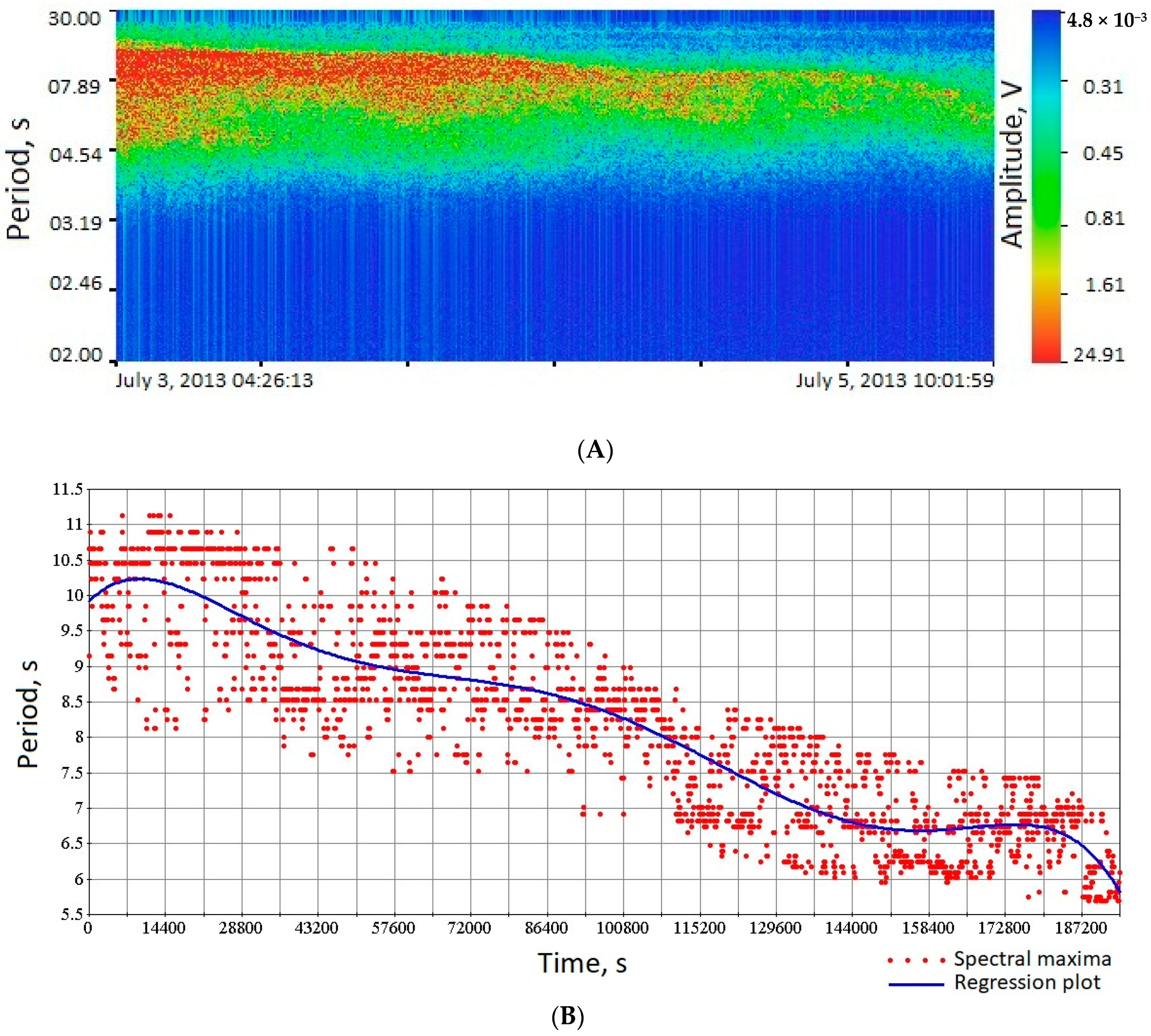
After processing and filtering the signal, the signal spectrograms were constructed for all selected fragments. Then, with a step of 60 samples (1 min), the frequency maxima of the region, corresponding to wind waves, were singled out. In order to visually represent the period change nature, on the obtained spectral maxima, by means of regression analysis, the functions were constructed, which were the polynomials of the 6th degree, since they adequately described the nature of the changes. Figure 2 and Figure 3 show the spectrograms of some record fragments and the corresponding regression curves.
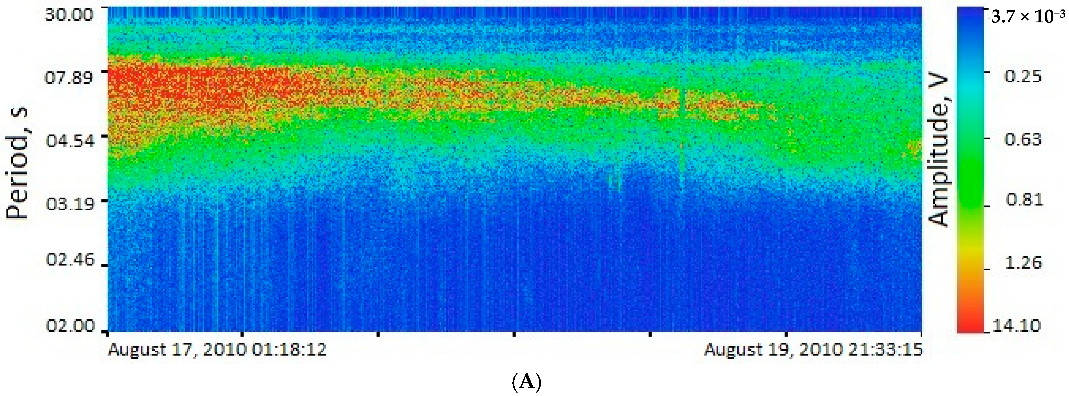
As we can see from Figure 2 and Figure 3, changes in the period of wind waves in all cases had a different character. In the case of the regression curves, presented in Figure 2, there were areas of abrupt period change and areas in which the period practically did not change, while Figure 3 shows a fragment, in which the period decreased monotonically. Most likely, this effect was associated with the dispersion of wind waves and changes in the wind conditions in the part of the water area, where these waves were generated [16]. For more detailed description of the reasons for the wind waves period change, let us study this process while analyzing the data obtained during the movement of the KOMPASU typhoon in the Sea of Japan.
3. KOMPASU Typhoon Swell Waves Study
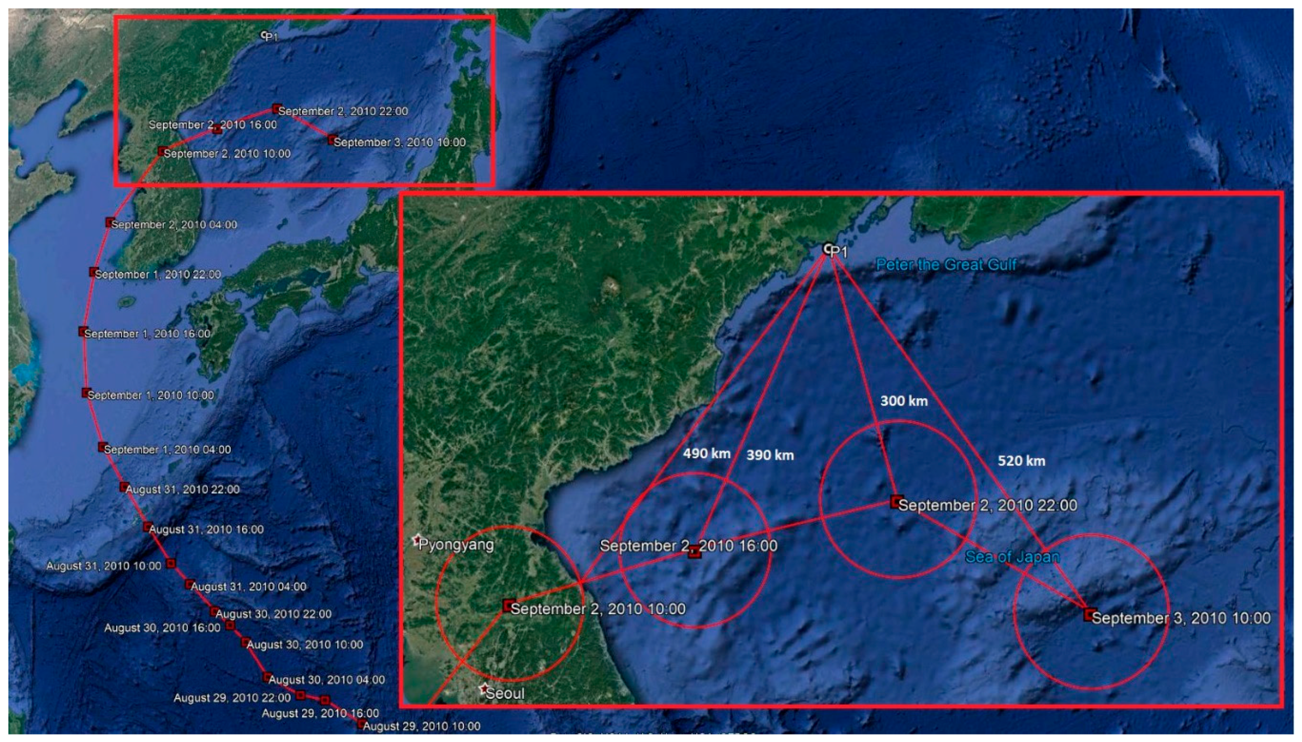
On 2 September 2010, typhoon KOMPASU entered the Sea of Japan, at 10:00 a.m. it passed over the territory of the Korean Peninsula; its trajectory is shown in Figure 4.
The dates and time are shown in Figure 4 at each point, where the typhoon passed. The typhoon began to enter the Sea of Japan on 2 September 2010 at 10:00, the last point of the typhoon trajectory—on 3 September 2010 at 04:00 (local time).
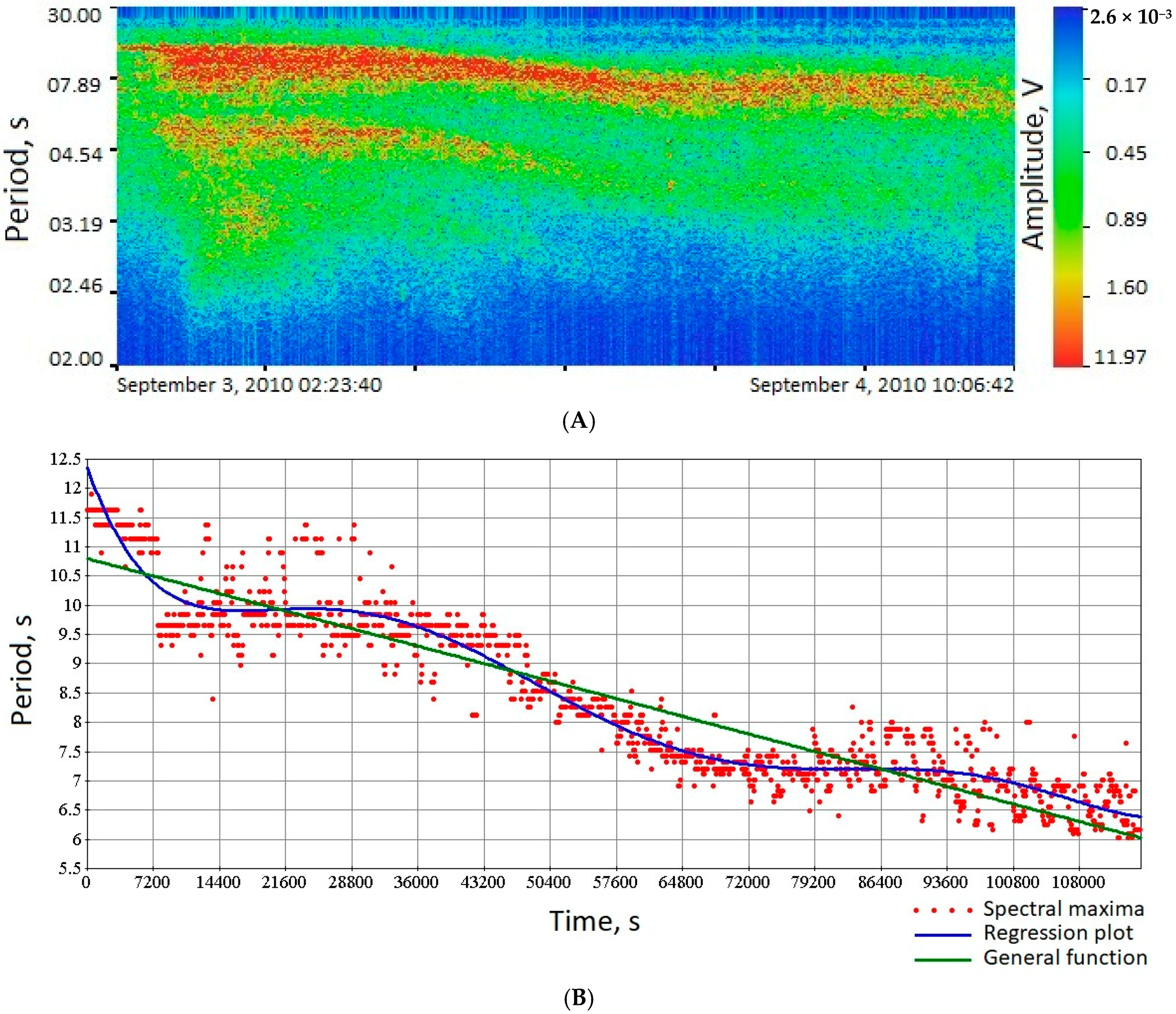
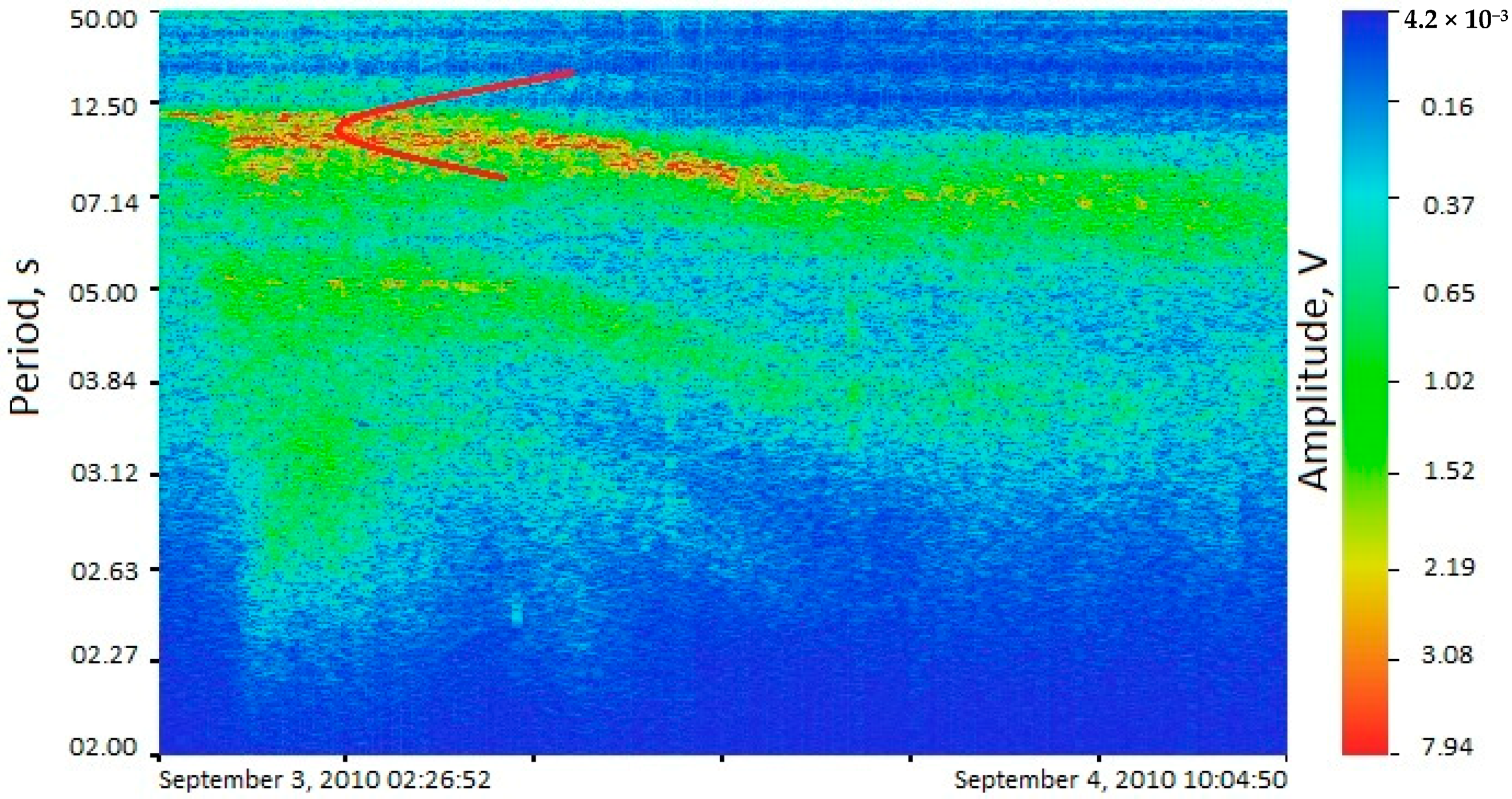
Figure 5 shows a spectrogram of the record of the laser meter of hydrosphere pressure variations located in Vityaz Bay during the typhoon passage and regression plot, constructed on the spectral maxima singled out from the signal spectrogram.
At the initial stage of Figure 2A, the period of the incoming swell was about 11.4 s. As we can see from the spectrogram, the lowest frequency process was nothing more than swell waves coming from the typhoon, which had a fairly wide range from 11.4 to 6 s. In this case, higher frequency processes were of no interest to us and they were local wind waves. Let us compare the general period variation function [17], constructed from the spectral maxima, with a more complex regression type that can better describe the effects associated with the typhoon passage. To estimate the polynomial regression and the general function of the period change, we used two criteria for the regression analysis evaluation: the coefficient of determination R2 (equal to 1 in the ideal case) and the standard deviation S (equal to 0 in the ideal case). The values of these quantities are given in Table 1.
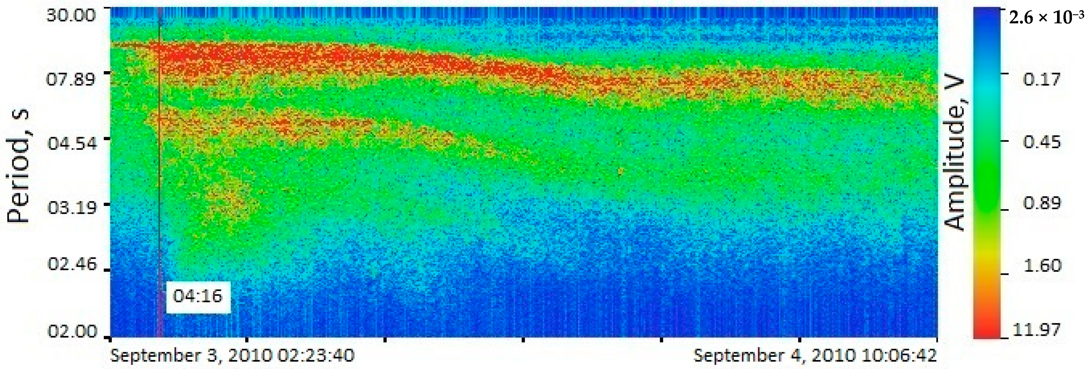
As we can see from Table 1, the difference between two regressions was not significant, but was still present. Now let us take a closer look at the effects of period change, associated with the propagation of this typhoon. Let us calculate the time of swell propagation from the supposed source. Let us use the formula for the propagation velocity in the deep sea approximation c = gT/2π. Entering the period 11.4 s into the express (A) spectrogram of the record of the laser meter of hydrosphere pressure variations and (B) regression plot, constructed on the spectral maxima singled out from the signal spectrogram. Taking into account that we need the group propagation velocity, and not the phase one, i.e., cgr = cph/2, we estimated that the propagation speed in this case will be 8.98 m/s. Considering the distance of 390 km from the 2nd typhoon point in Peter the Great Bay, we found that the swell waves should come to Vityaz Bay in 43,870 s or 12.18 h. If we take into account that the typhoon came to the point on 2 September 2010 at 16:00, then, according to calculations, the swell waves should come to the place of registration on 3 September 2010 at about 04:00. Figure 6 shows a spectrogram with a mark of the main group of swell waves arrival to Vityaz Bay. Considering the estimated time of arrival, the coincidence is very good, but as we can see, before this time there is also swell with a period of 11.4 s on the spectrogram. We could explain this arrival by the fact that the swell waves began to form earlier than the calculated point, and, taking into account the time of 2 h, this point was approximately 60 km down the typhoon trajectory.
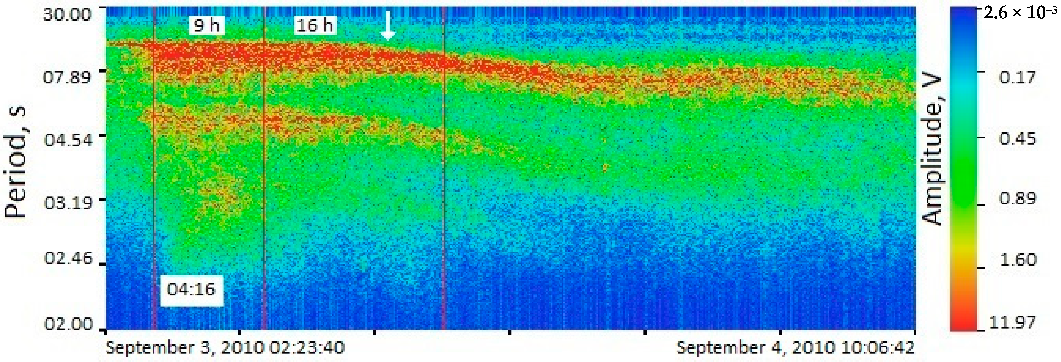
Let us consider points 3 and 4 (final) of the typhoon movement, the distance from each of them to Vityaz Bay is 300 and 520 km. Considering the swell propagation speed, we found that the swell waves should propagate to the registration point for 9 and 16 h (Figure 7). In theory, all this time the typhoon wind conditions should feed the swell waves with energy, and the wave period should not decrease during this period.
Let us look at Figure 7. It is assumed that at the selected time intervals, the swell waves with a period of 11.4 s should be fed, and the period of the waves should not change. However, as we can see from the 16-h fragment, the wave period decreased (shown by the white arrow). This effect could have several explanations: (1) change in the wind conditions. Indeed, according to the typhoon data, when passing points 2 and 4, the typhoon wind speed changed from 23 to 15 m/s, which could affect the period changes. (2) Doppler effect. If we look at the typhoon trajectory, we can clearly see that from point 2 to point 3 the typhoon moved almost parallel to the section line of Vityaz Bay, and at point 4 it moved from it at a certain angle, which in turn could also influence the changes in the wave period.
Let us consider the influence of the typhoon movement direction, its speed and the angle of its movement direction to the receiver. The starting point for calculations was the point where the typhoon enters the Sea of Japan, i.e., a point located in the middle of the section between point 1 and 2 of the typhoon passage. The typhoon was at this point on 2 September 2010 at 13:00; we took this point as 0, the time from this point we counted in seconds. Table 2 and Table 3 show the parameters of the typhoon movement and wind speed during its movement.
We also wrote information on wind speed into Table 3.
Let us calculate the changes in the wave period by the formula:
where: is initial value of the wave period, is the typhoon movement speed, and c is wind wave speed. Figure 8 shows the calculated graph of the possible period change due to the Doppler effect and data on the wind speed change.
According to the graph of the swell period change, presented in Figure 8, we compiled a table of the swell waves periods on the time of the typhoon movement, every 3 h, starting from the starting point in the water area (2 September 2010 at 13:00), taken as 0, we also indicate the distance to the receiver, propagation time, time at a point, and time of arrival to the receiver.
We can see from Table 4, that waves with periods of 9 and 11.5 s during the typhoon movement should arrive simultaneously, and ones with periods of 7.5 and 15 s. What is interesting is that 11.4 and 9 s were the main periods on the spectrogram, if we display the data from Table 4 on it, it will look like this (see Figure 9).
However, the time difference between the arrival of the main front of the swell waves in relation to the arrival of the 9 and 11.5 s waves, theoretically generated by the typhoon movement, was 3 h. The question arises whether this effect can occur not in the very center of the typhoon movement, but in its vicinity. Let us estimate the calculation error in kilometers, i.e., the distances that the waves of these periods would pass in 3 h. Error estimates are given in Table 5.
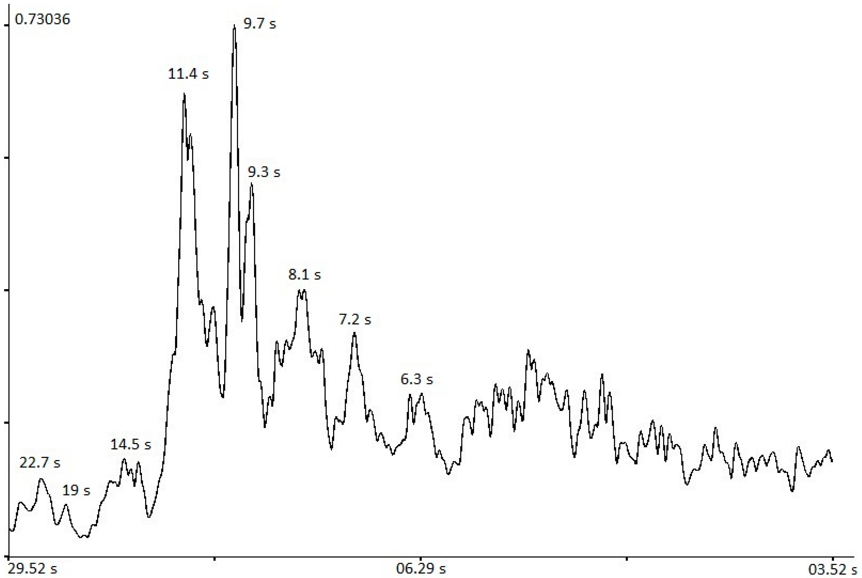
Initially, it was said that the typhoon had a radius of 90 km; based on the data in Table 5, we could assume that simultaneous arrival of the swell front with periods of 9 and 11.5 s caused by the Doppler effect for this typhoon was possible only in one case: when this effect was formed by the leading front of the typhoon or near it. There is a question: if this effect really exists, then, as we already mentioned, when moving to the last point, the typhoon should initiate waves with a period of 18 s, and there were none of them on the spectrogram. We can explain this by a decrease in wind speed, which is shown in Figure 7. Thus, the waves with a period of 18 s will have very small amplitude and be invisible against the background of other processes. In support of this assumption, we should consider the wave spectrum in the interval from the moment of the first arrival of the wave packet to the beginning of the decrease in the swell period, shown in Figure 10.
To begin with, we should say that the wave condition is a complex and non-stationary process, the period is constantly changing within small limits and it is impossible to talk about any exact figures, only within certain limits. As we can see from Figure 9, the periods of the main harmonics approximately coincided with the calculated periods from Table 4, which may testify in favor of the assumption that a number of harmonics of swell waves are formed during the movement of a typhoon leading front. We can also see the harmonic of the period 19 s on the spectrum, which, in turn, can confirm the assumption about the small amplitude of these waves due to the wind decrease, and their formation when the typhoon moved in the direction from the source.
Of course, there is also a simple explanation for the simultaneous arrival of waves with periods of 9 and 11.5 to the receiving point. This will happen if 9 s waves originated at a point, located between the first and second points of the typhoon trajectory, indicated in Figure 4, at 490 km from the receiving point. The typhoon was at the indicated point on 2 September 2010 at 13:00. Then the waves of the specified period will reach the receiving point on 3 September 2010 at 6:00. The waves with a period of 11.5 s should be generated in the second point of the typhoon trajectory, at the distance of 390 km from the receiver, and will come to the receiving point on 3 September 2010 at 4:00. The difference of 2 h can also be leveled with the typhoon radius of 90 km, since the error for the period of 9 s will be 50 km. There is an even simpler explanation, which is in the concept itself of the swell waves group propagation speed. When a typhoon affects the water surface, the waves of a sufficiently small period begin to appear, which propagate with a phase speed; over time, the waves period increases and, reaching a maximum during propagation, begins to capture waves of a close period; they, in turn, begin to capture waves of a period close to them. As a result, the entire wave packet propagates at the speed of the maximum possible period, and at a speed 2 times lower than the phase one, i.e., with group speed. However, not all periods can capture each other, which is why such a “comb” of harmonics appeared in the spectrum. We can easily show the formation of wave groups by making calculations by a simple equation.
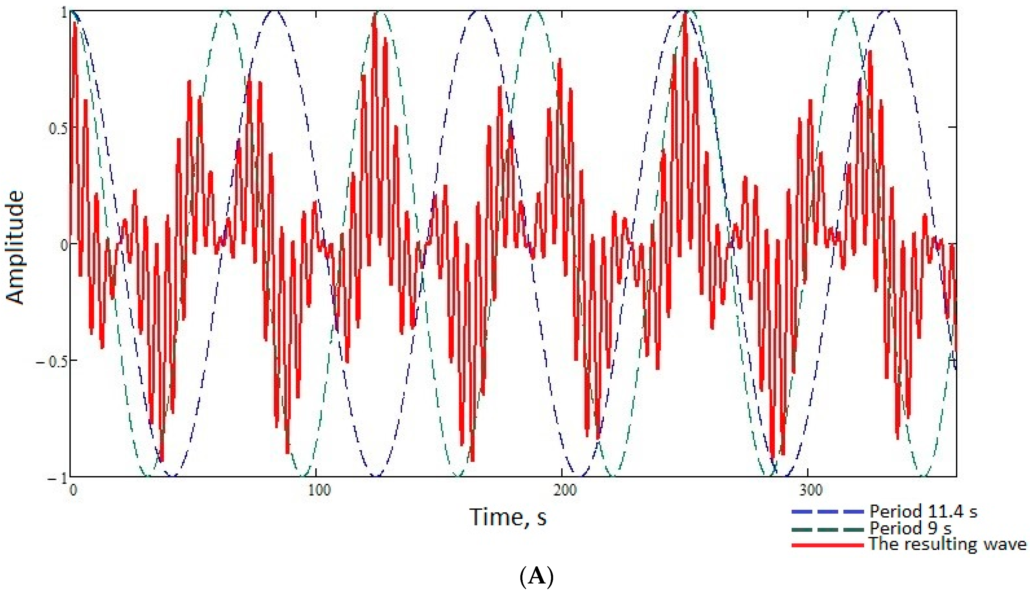
Figure 11 shows an example of the formation of waves with periods of 11.4, 9 and 7 s, the main period of which was 11.4 s, and propagating with the group speed.
Now let us consider the question of how, from a fragment with a changing period, can we determine the distance to the place of origin of the wave process. From the spectrogram, shown in Figure 6, we can see that about 13 h passed from the beginning of the period decrease to its final value, and to determine the distance to the source, we could use the simple formula , where is the time interval in seconds and is the group propagation speed. In this case, in the formula for the group speed, we should substitute the largest period, from which the decrease begins, the final period in this case did not matter, we can show this using the general function of period change. According to [18], we wrote down the general formula for period change as:
Substitute this expression into the formula for finding the distance
After transformations we get
Taking into account the value of the coefficient
, equal to then, with the term can be neglected, and then we get the following
expression:
This is nothing other than the group speed multiplied by the time interval. Thus, knowing that the period began to change from 11.4 s and its complete change occurred in about 13 h (46,800 s), we get that the source should be located at the distance of 416 km, which practically corresponded to point 2 of the typhoon passage. Thus, we could claim that the linear change in the swell period was nothing other than the usual dispersion of propagation, in which waves with a large period, having a high speed, came first, and with a smaller one, arrived last.
4. Shelf Infragravity Sea Waves
There are still various points of view on the nature of oscillations and waves in the range of periods from 20–30 s to 8–10 min, recorded in the sea, each of which finds a balanced confirmation in the observed experimental data. The considered range of periods corresponds to the so-called “Infragravitational noise of the Earth”, the origin of which may be associated with various processes in all geospheres, any of which is suitable for explaining the appearance of oscillations and waves of this periods range. In this paper, we will pay attention to the mechanism of occurrence of the considered periods range oscillations related to infragravity sea waves, arising on the shelf as a result of the action of sea gravity waves, i.e., so-called wind surface waves or swell waves. When interpreting the obtained results, we used the experimental data from the laser meter of hydrosphere pressure variations, installed on the shelf of the Sea of Japan at the depth of 27 m to the south from Shultz Cape (see Figure 12).
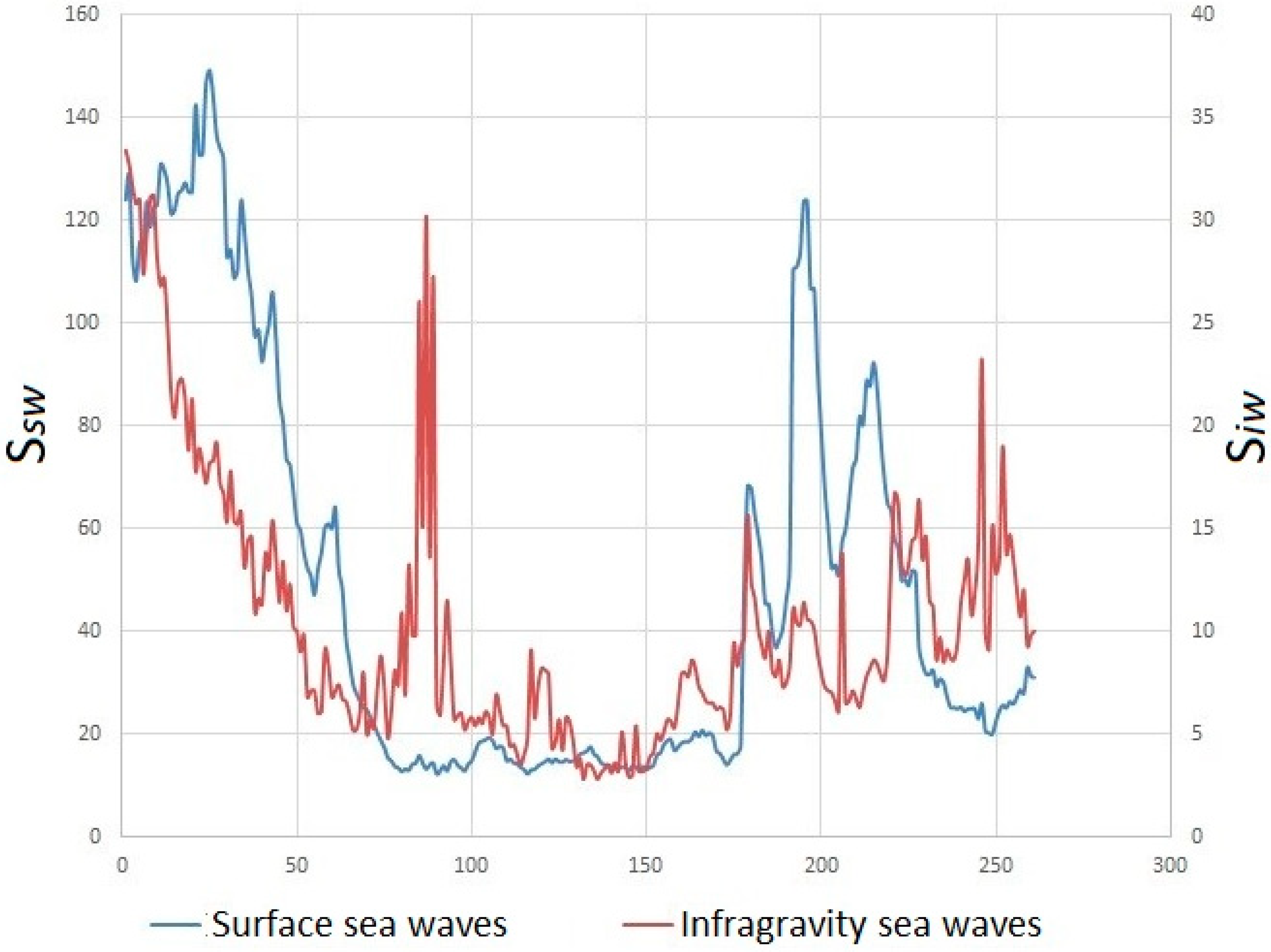
Hourly data files from the laser meter of hydrosphere pressure variations were filtered by a low frequency Hamming filter, followed by decimation of up to 2 s, then the decimated experimental data were filtered by a high-frequency Hamming filter with a cutoff frequency of 0.002 Hz (8.3 min) and length of 2500. In the process of spectral processing of the filtered hour files, significant peaks were singled out in the range of surface sea wind waves (periods from 1 to 20 s) and in the range of infragravity sea waves (periods from 20 s to 8 min). Additionally, the relative energy was determined from the harmonics values of all spectral components in the given period ranges (1–20 s and 20 s–8 min). Thus, the values of the total relative energy were obtained in the range of sea surface wind waves () and sea infragravity waves (). In total, 267 files of one-hour duration each were processed, i.e., duration of the continuous series of observations was a little over 11 days. In the considered observation interval, the values of the periods and amplitudes of surface sea waves (swell and wind sea waves) changed significantly, which allowed us to determine the relationship between infragravity sea waves and surface sea waves. Figure 13 shows the graphs of changes in the relative energy of surface sea waves (1–20 s) and the relative energy of infragravity sea waves (20 s–8 min). As we can see from this figure, the relative energy of infragravity sea waves generally repeats the curves of surface sea waves.
Some abrupt increase in the relative energy of infragravity sea waves in comparison with the relative energy of surface sea waves (abrupt surges in files 87–91) was associated with the presence of solitary waves in the records of the laser meter of hydrosphere pressure variations, which, upon spectral processing, significantly increased the relative energy in the infragravity range and did not increase the relative energy in the sea wave range.
5. Conclusions
After the studies in the range of gravity sea waves, the following conclusions could be drawn: (1) When comparing the polynomial regression and the general function of the period change, with the help the analysis we conducted of the change in the swell waves periods during the passage of the typhoon through the Sea of Japan, we determined that the difference in the quality of describing this process was insignificant.
Thus, to describe wave processes of this type, the general period change function could be used instead of high-order polynomial regressions. (2) The assumption about the generation of waves of a certain period when the typhoon moved at a certain speed at an angle to the receiver looked convincing, if we assume that these periods are formed by the leading front of the typhoon, while the wind condition in the typhoon, which can affect the amplitude of these wave periods, plays an important role. This effect could also explain the variety of periods of swell waves, created by the typhoon. (3) Separate peaks of certain periods in the typhoon spectrum and simultaneous arrival to the registration point could be explained by the group propagation of swell waves, when waves with the largest period captured the waves with a period close to their own, and the entire group propagated at a speed of the largest period, which was two times less than the phase speed. (4) Using the formula for the group speed of wave propagation in deep water conditions, knowing the duration of the interval of period change from maximum to minimum, we could quite accurately determine the distance to the source, from which these waves came. The linear effect of the period decrease was associated exclusively with dispersion during their propagation. We established that change in the total energy of the sea infragravity waves (20 s–8 min) correlated with change in the total energy of sea gravity waves (2–20 s), which testified in favor of the theory of generation of sea infragravity waves by gravity sea waves. We discovered powerful solitary perturbations of the sea surface of considerable duration, exceeding the amplitude of local tides. According to some indications, they can be related to rogue waves, but with a big difference in the duration of the process. Further research in this direction is extremely necessary to establish the physics of their origin, development, and transformation.
Author Contributions
G.D.—problem statement, experimental work experimental data processing, guidance in writing an article. S.D.—processing of experimental data, calculations, creation of graphic material dedicated to infragravity sea waves. S.B.—processing of experimental data, calculations, creation of graphic material dedicated to Swell Waves. All authors have read and agreed to the published version of the manuscript.
Funding
This work was carried out with partial financial support of the topic AAAA-A20-120021990003-3 “Research of fundamental foundations of the origin, development, transformation and interaction of hydroacoustic, hydrophysical and geophysical fields of the World Ocean”.
Acknowledgments
We would like to express our deep gratitude to all employees of the Physics of Geospheres laboratory.
Conflicts of Interest
The authors declare no conflict of interest.
References
- Newton, I. The Principia: Mathematical Principles of Natural Philosophy; Cohen, I.B.; Whitman, A., Translators; University of California Press: Berkeley, CA, USA, 1999. [Google Scholar]
- Gardner, C.S.; Greene, J.M.; Kruskal, M.D.; Miura, R.M. Method for solving the Korteweg-de Vries equation. Phys. Rev. Lett. 1967, 19, 1095–1097. [Google Scholar] [CrossRef]
- Benjamin, T.B.; Feir, J.E. The disintegration of wave train on deep water. J. Fluid Mech. 1967, 27, 417–430. [Google Scholar] [CrossRef]
- Longuet-Higgins, M.S.; Cleaver, R.P. Crest instabilities of gravity waves. Part 1. The almost-highest wave. J. Fluid Mech. 1994, 258, 115–129. [Google Scholar] [CrossRef]
- Lounge-Higgins, M.S. The instabilities of gravity waves of infinite amplitude in deep sea. II. Subharmonics. Proc. R. Soc. Lond. Ser. A 1978, 360, 489–505. [Google Scholar]
- Lounge-Higgins, M.S.; Smith, N.D. An experiment on third order resonant wave interactions. J. Fluid Mech. 1966, 25, 417–436. [Google Scholar] [CrossRef]
- Hasselmann, K. On the nonlinear energy transfer in gravity-wave spectrum. General theory. J. Fluid Mech. 1962, 12, 481–500. [Google Scholar] [CrossRef]
- Hasselmann, K. Weak-interaction theory of ocean waves. In Basic Development in Fluid Dynamics; Academic Press: New York, NY, USA, 1968; pp. 117–182. [Google Scholar]
- Caponi, E.A.; Saffman, P.G.; Yuen, H.C. Instability and confinedchaos in a nonlinear dispersion wave system. Phys. Fluids 1982, 25, 2159–2166. [Google Scholar] [CrossRef] [Green Version]
- Tolman, H.L.; Balasubramaniyan, B.; Burroughs, L.D.; Chalikov, D.V.; Chao, Y.Y.; Chen, H.S.; Gerald, V.M. Development and implementation of wind generated ocean surface models at NCEP. Weath. Forecast. 2002, 17, 311–333. [Google Scholar] [CrossRef]
- Tolman, H.L. Numerics in wind wave models. In Proceedings of the ECMWF Workshop on Ocean Wave Forecasting, Reading, UK, 2–4 July 2001; pp. 5–14. [Google Scholar]
- Donelan, M.A. A nonlinear dissipation function due to wave breaking. In Proceedings of the ECMWF Workshop on Ocean Wave Forecasting, Reading, UK, 2–4 July 2001; pp. 87–94. [Google Scholar]
- Dolgikh, S.G.; Budrin, S.S.; Plotnikov, A.A. Laser meter for hydrosphere pressure variations with a mechanical temperature compensation system. Oceanology 2017, 57, 600–604. [Google Scholar] [CrossRef]
- Dolgikh, G.I.; Piao, S.; Budrin, S.S.; Song, Y.; Dolgikh, S.G.; Chupin, V.A.; Yakovenko, S.V.; Dong, Y.; Wang, X. Study of low-frequency hydroacoustic waves behavior at the shelf of decreasing depth. Appl. Sci. 2020, 10, 3183. [Google Scholar] [CrossRef]
- Dolgikh, G.; Chupin, V.; Gusev, E. Microseisms of the “Voice of the Sea”. IEEE Geosci. Remote Sens. Lett. 2020, 15, 750–754. [Google Scholar] [CrossRef]
- Dolgikh, G.I.; Budrin, S.S.; Dolgikh, S.G.; Ovcharenko, V.V.; Plotnikov, A.A.; Chupin, V.A.; Shvets, V.A.; Yakovenko, S.V. Dynamics of wind waves during propagation over a shelf of decreasing depth. Dokl. Earth Sci. 2012, 447, 1322–1326. [Google Scholar] [CrossRef]
- Budrin, S.S.; Dolgikh, G.I.; Dolgikh, S.G.; Yaroshchuk, E.I. Studying the variability of the wind wave period. Russ. Meteorol. Hydrol. 2014, 39, 47–52. [Google Scholar] [CrossRef]
- Dolgikh, G.I.; Budrin, S.S. Some Regularities in the Dynamics of the Periods of Sea Wind Waves. Dokl. Earth Sci. 2016, 468, 536–539. [Google Scholar] [CrossRef]
Figure 1.
External view (A) and optical scheme of a laser meter of hydrosphere pressure variations (B).
Figure 1.
External view (A) and optical scheme of a laser meter of hydrosphere pressure variations (B).

Figure 2.
(A) Swell wave spectrogram recorded by a laser meter of hydrosphere pressure variations in the period from 3 July to 5 July 2013 and (B) regression plot, constructed on the spectral maxima singled out from the signal spectrogram recorded in the period from 3 July to 5 July 2013.
Figure 2.
(A) Swell wave spectrogram recorded by a laser meter of hydrosphere pressure variations in the period from 3 July to 5 July 2013 and (B) regression plot, constructed on the spectral maxima singled out from the signal spectrogram recorded in the period from 3 July to 5 July 2013.

Figure 3.
(A) Swell wave spectrogram recorded by a laser meter of hydrosphere pressure variations in the period from 17 August to 19 August 2010 and (B) regression plot, constructed on the spectral maxima singled out from the signal spectrogram recorded in the period from 17 August to 19 August 2010.


Figure 4.
Typhoon KOMPASU trajectory. Point P1—“Vityaz” Bay, the points of the typhoon passage are indicated by the date and time (local time), red circles indicate areas with winds exceeding 18 m/s, the area radius is 90 km. Distances to “Vityaz” Bay are noted for three points of the typhoon distribution.

Figure 5.
(A) Spectrogram of the record of the laser meter of hydrosphere pressure variations located in Vityaz Bay during the KOMPASU typhoon passage and (B) regression plot, constructed on the spectral maxima singled out from the signal spectrogram.
Figure 5.
(A) Spectrogram of the record of the laser meter of hydrosphere pressure variations located in Vityaz Bay during the KOMPASU typhoon passage and (B) regression plot, constructed on the spectral maxima singled out from the signal spectrogram.

Figure 6.
Time of swell waves arrival to the registration point.

Figure 7.
Segments of swell waves arrival time from points 3 and 4 of the typhoon trajectory.

Figure 8.
Graph of the swell period change on the typhoon speed and the angle of direction to the receiver (left scale, red curve), change in the typhoon wind speed (right scale, blue curve).
Figure 8.
Graph of the swell period change on the typhoon speed and the angle of direction to the receiver (left scale, red curve), change in the typhoon wind speed (right scale, blue curve).

Figure 9.
Calculated Doppler effect.

Figure 10.
Swell waves spectrum.

Figure 11.
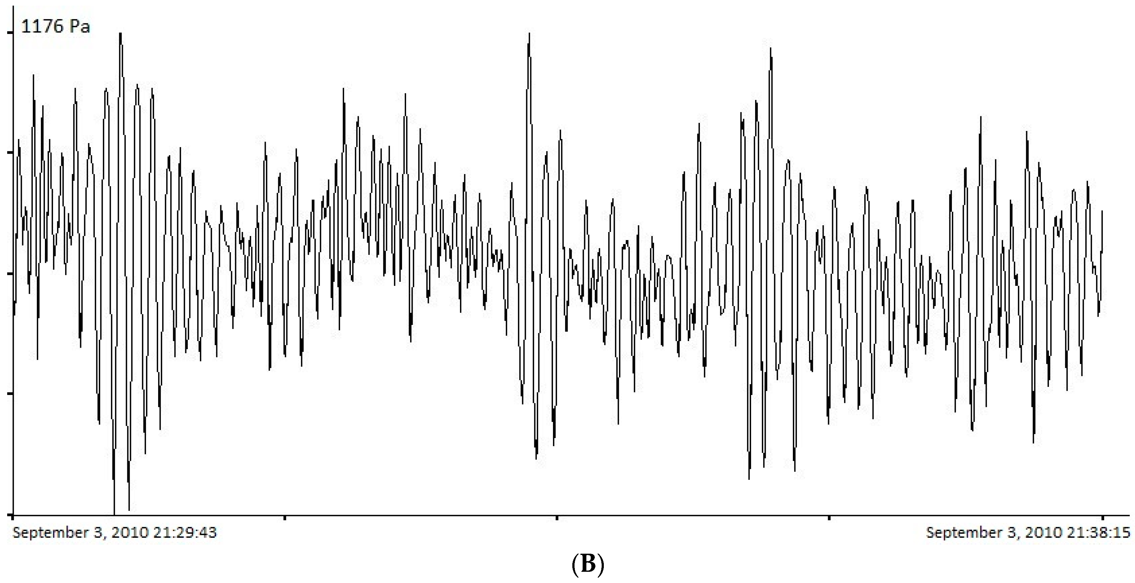
(A) Group of waves formed with a period of 11.4 s, which captured a wave with a period of 9 s, which, in turn, captured a wave with a period of 7 s (11.4 s enveloping curve—blue dotted line, 9 s enveloping curve—green dotted line, and red line is the resulting wave, consisting of three wave periods). (B) Record fragment of the laser meter of hydrosphere pressure variations of the typhoon arrival area, shown for comparison.
Figure 11.
(A) Group of waves formed with a period of 11.4 s, which captured a wave with a period of 9 s, which, in turn, captured a wave with a period of 7 s (11.4 s enveloping curve—blue dotted line, 9 s enveloping curve—green dotted line, and red line is the resulting wave, consisting of three wave periods). (B) Record fragment of the laser meter of hydrosphere pressure variations of the typhoon arrival area, shown for comparison.


Figure 12.
Map of locations of the laser meter of hydrosphere pressure variations (LMHPVs) and the laser strainmeter (LS).
Figure 12.
Map of locations of the laser meter of hydrosphere pressure variations (LMHPVs) and the laser strainmeter (LS).

Figure 13.
Change in the relative energy of surface sea waves () and infragravity sea waves ( ).


Table 1.
Regression analysis evaluation criteria.
| R2 | S | |
|---|---|---|
| Polynomial regression | 0.926 | 0.4 |
| Period function | 0.865 | 0.54 |
| Difference | 0.061 | 0.14 |
Table 2.
Typhoon parameters.
| Time, s | Speed, m/s | Angle, Degrees |
|---|---|---|
| 0 | 9.76 | 140 |
| 10,800 | 9.81 | 130 |
| 32,400 | 11.2 | 90 |
| 54,000 | 11.9 | 30 |
Table 3.
Wind data.
| Time, s | Wind Speed, m/s |
|---|---|
| 0 | 23 |
| 10,800 | 20 |
| 32,400 | 18 |
| 54,000 | 15 |
Table 4.
Estimated data.
| Time on Graph, s | Period, s | Propagation Time, h | Time at a Point | Arrival Time |
|---|---|---|---|---|
| 0 | 6.8 | 24 | 2 September 2010 13:00 | 3 September 2010 13:00 |
| 10,800 | 7.5 | 18 | 2 September 2010 16:00 | 3 September 2010 10:00 |
| 21,600 | 9 | 12 | 2 September 2010 19:00 | 3 September 2010 07:00 |
| 32,400 | 11.5 | 9 | 2 September 2010 22:00 | 3 September 2010 07:00 |
| 43,200 | 15 | 9 | 3 September 2010 01:00 | 3 September 2010 10:00 |
| 54,000 | 18 | 10 | 3 September 2010 04:00 | 3 September 2010 14:00 |
Table 5.
Error estimates.
| Period, s | Propagation Speed, m/s | Distance, km |
|---|---|---|
| 9 | 7 | 75 |
| 11.5 | 8.9 | 96 |
© 2020 by the authors. Licensee MDPI, Basel, Switzerland. This article is an open access article distributed under the terms and conditions of the Creative Commons Attribution (CC BY) license (http://creativecommons.org/licenses/by/4.0/).
Share and Cite
MDPI and ACS Style
Dolgikh, G.; Budrin, S.; Dolgikh, S. Fluctuations of the Sea Level, Caused by Gravitational and Infra–Gravitational Sea Waves. J. Mar. Sci. Eng. 2020, 8, 796. https://doi.org/10.3390/jmse8100796
AMA Style
Dolgikh G, Budrin S, Dolgikh S. Fluctuations of the Sea Level, Caused by Gravitational and Infra–Gravitational Sea Waves. Journal of Marine Science and Engineering. 2020; 8(10):796. https://doi.org/10.3390/jmse8100796
Chicago/Turabian StyleDolgikh, Grigory, Sergey Budrin, and Stanislav Dolgikh. 2020. "Fluctuations of the Sea Level, Caused by Gravitational and Infra–Gravitational Sea Waves" Journal of Marine Science and Engineering 8, no. 10: 796. https://doi.org/10.3390/jmse8100796
Note that from the first issue of 2016, this journal uses article numbers instead of page numbers. See further details here.