Wind Turbulence Statistics of the Atmospheric Inertial Sublayer under Near-Neutral Conditions

Abstract

The inertial sublayer comprises a considerable and critical portion of the turbulent atmospheric boundary layer. The mean windward velocity profile is described comprehensively by the Monin–Obukhov similarity theory, which is equivalent to the logarithmic law of the wall in the wind tunnel boundary layer. Similar logarithmic relations have been recently proposed to correlate turbulent velocity variances with height based on Townsend’s attached-eddy theory. The theory is particularly valid for high Reynolds-number flows, for example, atmospheric flow. However, the correlations have not been thoroughly examined, and a well-established model cannot be reached for all turbulent variances similar to the law of the wall of the mean-velocity. Moreover, the effect of atmospheric thermal condition on Townsend’s model has not been determined. In this research, we examined a dataset of free wind flow under a near-neutral range of atmospheric stability conditions. The results of the mean velocity reproduce the law of the wall with a slope of $2.45$ and intercept of $-13.5$. The turbulent velocity variances were fitted by logarithmic profiles consistent with those in the literature. The windward and crosswind velocity variances obtained the average slopes of $-1.3$ and $-1.7$, respectively. The slopes and intercepts generally increased away from the neutral state. Meanwhile, the vertical velocity and temperature variances reached the ground-level values of $1.6$ and $7.8$, respectively, under the neutral condition. The authors expect this article to be a groundwork for a general model on the vertical profiles of turbulent statistics under all atmospheric stability conditions.

1. Introduction

The inertial sublayer (IS), overlap layer, or logarithmic layer is characterised by its solid logarithmic mean-velocity profile. Employing this logarithmic velocity equation, known as the law of the wall, provides a cost effective near-wall treatment in computational fluid dynamics. In engineering applications, the turbulence level can be predicted, leading to meaningful drag reduction initiatives. Hence, the law was subjected to intensive investigation [1,2,3] to improve its accuracy and widen its scope of validity.

Townsend’s attached-eddy model [4,5] predicts the size and density of population of the turbulent coherent structures (TCS) in the IS at high Reynolds numbers. A comprehensive discussion on the model can be found in [6]. The most important argument in Townsend’s model is the hypothesis in which the eddy population is inversely proportional to the distance from the wall. The model, together with the turbulent-eddy visualisations of Head and Bandyopadhyay [7], inspired mathematicians to derive expressions for turbulence statistics. Perry et al. [8,9] devised a model to predict turbulence statistics (mean velocity, turbulence intensity, spectrum, and temperature) by applying the attached-eddy hypotheses to a forest of hairpin vortices of sizes proportional to their height from the wall. The model was further developed by Marusic [10] by utilising the vortex packet paradigm [11,12]. Marusic found the vortex packet to resemble the hypothesised attached eddies and prescribe turbulence statistics. The same configuration was suggested by Dennis and Nickels [13] through the 3-D velocity measurement of the turbulent boundary layer (TBL). Woodcock and Marusic [14] used the model to predict the variation of von Kármán’s constant with the Reynolds number. Cossu and Hwang [15,16,17] showed that the energy-containing motions at a given spanwise length-scale can self-sustain themselves by extracting energy directly from the mean flow even with the absence of any larger or smaller structures. They found the sizes of these energy containing motions to be proportional to their distances from the wall, which renders them to be good candidates as Townsend’s attached eddies. In addition, they anticipated each of these eddies to be composed of two elements, namely, a long streaky structure and a vortical structure. In the sublayer, these structures represent the low-speed streak and the quasi-streamwise vortices flanking it; in the logarithmic and wake layers, they represent the super-streak (VLSM, superstructure) and the hairpin vortex packets (LSMs) aligned along it.

One of the outcomes of Townsend’s model is the prediction of the logarithmic variation of turbulence variances ($\langle {u^{\prime +}}^2\rangle$, $\langle {v^{\prime +}}^2\rangle$ and $\langle {w^{\prime +}}^2\rangle$), that is,

$$\begin{array}{cc}\hfill \langle {u^{\prime +}}^2\rangle & =B_u-A_{u}ln(z/\delta ),\hfill \end{array}$$

(1)

$$\begin{array}{cc}\hfill \langle {v^{\prime +}}^2\rangle & =B_v-A_{v}ln(z/\delta ),\hfill \end{array}$$

(2)

$$\begin{array}{cc}\hfill \langle {w^{\prime +}}^2\rangle & =B_w,\hfill \end{array}$$

(3)

which are similar to the mean flow velocity profile (${\langle u\rangle }^{+}=Aln(z^{+})+B$), where ${u^{\prime +}}^2={u^{\prime }}^2/{u_{*}}^2$, ${v^{\prime +}}^2={v^{\prime }}^2/{u_{*}}^2$, ${w^{\prime +}}^2={w^{\prime }}^2/{u_{*}}^2$, $\langle u^{+}\rangle =\langle u\rangle /u_{*}$, and $z^{+}=z{u}_{*}/\nu$. In the equations, $u_{*}$ and $\nu$ represent the friction velocity and kinematic viscosity, $\delta$ is boundary-layer thickness, and As and Bs are constants. The A constant is known as the Townsend–Perry constant.

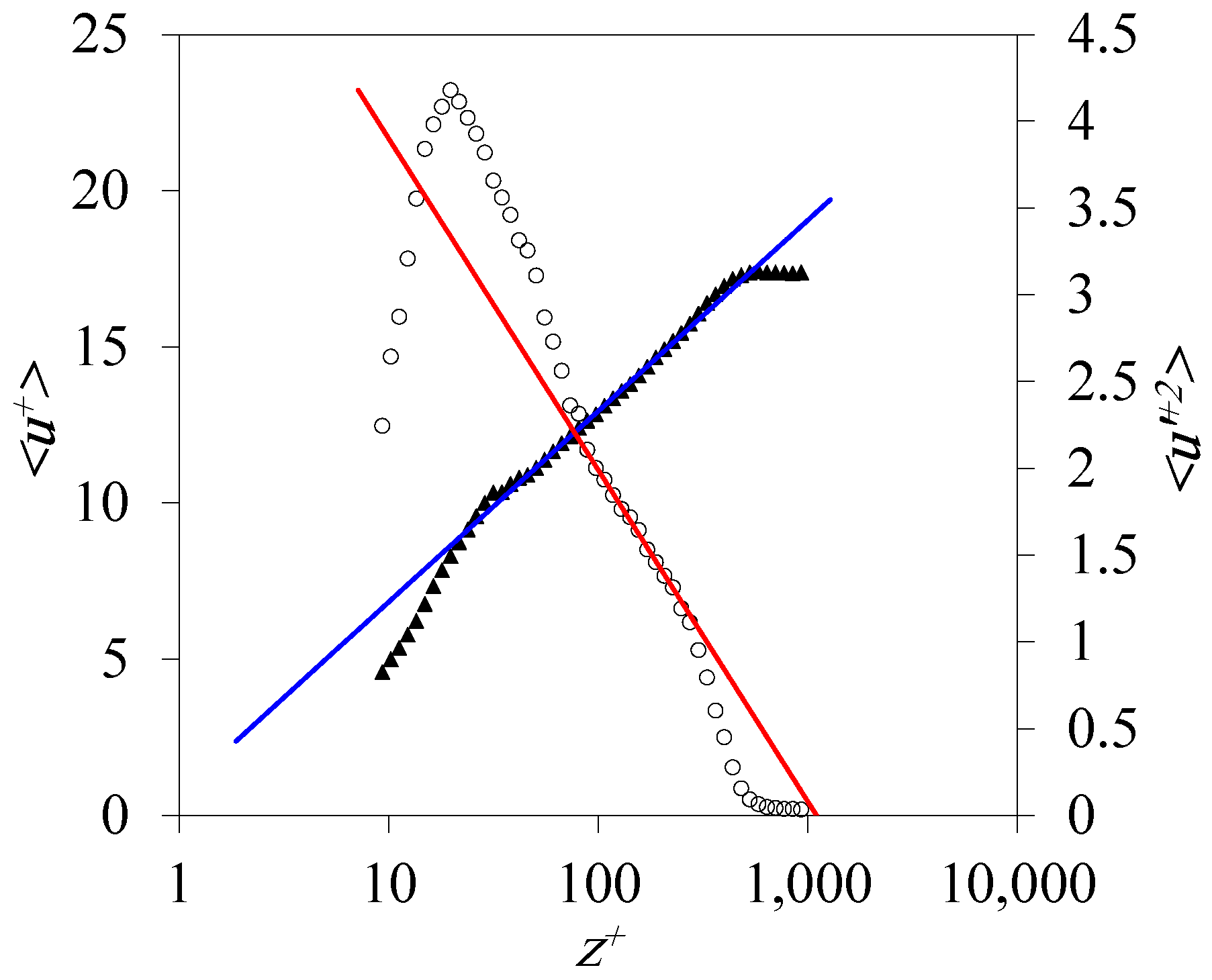
Hultmark [18] was the first researcher to provide experimental evidence of the logarithmic correlations in the IS. This discovery can be regarded somewhat late perhaps because, unlike the mean velocity profile, the logarithmic variance relations apply in a narrow zone within the IS, as shown in Figure 1. The low Reynolds number TBL data were acquired at the Pangkor Low Speed Wind Tunnel (PLSWT) [19]. Marusic et al. [2] proved the validity of the law by using a different high-Reynolds number ($R{e}_{*}=u_{*}\delta /\nu$) flows, including for the superpipe and atmospheric boundary layer. Meneveau and Marusic [20] extended the logarithmic behaviour to the higher order even moments (${u^{\prime +}}^4$, ${u^{\prime +}}^6$, etc.) and illustrated that the slopes (As) are insensitive to the Reynolds number, whereas the intercepts (Bs) are non-universal constants.

The turbulence intensity profiles in the IS are extremely important in the atmospheric boundary layer (ABL) because the IS largely grows at high-Re. In the ABL, the IS can extend to tens of meters above the ground surface and hence dominates the flow over man-made structures and urban areas. The mean-velocity profile in the ABL is described comprehensively by Monin–Obukhov similarity theory [21] in cooperation with the Businger–Dyer corrections [22]. The profiles of turbulence statistics ($\langle u^{\prime +}\rangle$, $\langle v^{\prime +}\rangle$ and $\langle w^{\prime +}\rangle$) in the ABL received similar attention [23,24,25]. The parameters increase under both stable and convective (unstable) conditions and settle under neutral conditions at values fluctuating around 2 [26,27,28]. However, the above studies were based on atmospheric stability as a sole independent parameter. Moreover, the researchers were neither aware of the TCS nor the logarithmic relations in the IS. The turbulence structure of the ABL, which is the core of the attached-eddy model, is largely similar to the canonical wind tunnel boundary layer. The IS is dominated by vortex packets and super-streaks, both scaling with boundary-layer heights [29]. A vortex packet can reach $2-3\delta$ [30] long, while a super-streak extends to $12\delta$ [31]. These TCSs are sensitive to atmospheric stability conditions [23,32,33]. Consequently, the validity of Townsend’s theory, and hence the applicability of the logarithmic relations under stable and convective situations, is questioned.

Plenty of existing studies were devoted to the change in turbulence variances with atmospheric stability. However, to our knowledge, none of them addressed vertical profiles as part of Townsend’s model. The target of this research is to utilise Townsend’s theory to describe turbulence statistics in the ABL under different stability conditions. In other words, our aim is to investigate the variation of the logarithmic relations’ constants with atmospheric stability. Accordingly, a free atmospheric flow dataset was employed to incorporate measurements at three levels and cover a near-neutral range of stability conditions. The findings may help improve the current turbulence models and hence enhance flow simulation accuracy and increase civil and mechanical structures durability.

A wide variety of mathematical techniques can be employed to detect TCS and deduce their geometries. A willing method is the wavelet transform [34,35]. The wavelet transform is a time-localised version of the typical time–frequency sinusoidal transforms, for example, Fourier transform. That is, the wavelet transform extracts the time traces of selected TCS scales. Moreover, a full power spectrum can be derived from the energy content in each time scale. The vortex packet and super-streak appear in this power spectrum as two peaks similar to that in the Fourier power spectrum [32,36]. Thus, their length scales can be detected. The remainder of this paper is organised as follows. Section 2 describes the dataset utilised in this study and details the methodology for analysis. Section 3 presents the results and discussion. Section 4 summarises the outcomes of the study.

2. Method

The ABL data from the Marine Ecosystem Research Centre (EKOMAR) third experimental campaign [32], namely the northern dataset, was used in this study. The EKOMAR site (2${}^{\circ }$34${}^{\prime }$42.11${}^{″}$ N, 103${}^{\circ }$48${}^{\prime }$21.05${}^{″}$ E) lies on the east coast of Malaysia, approximately 22 km north of the town of Mersing. The location allows the acquisition of undisturbed ABL data of the flow from the sea. The measurement campaign started on 7 November 2017 and lasted 20 days. Three three-dimensional ultrasonic anemometers were utilised: (1) a CSAT-3B anemometer (Campbell Scientific, Logan, UT, USA; 0.001 m s${}^{-1}$ and 0.002 ${}^{\circ }$C resolution and ±0.08 m s${}^{-1}$ and ±2 ${}^{\circ }$C accuracy) was at 1.7 m above ground level, and (2) two YOUNG 81000 anemometers (R.M. YOUNG, Traverse City, MI, USA; 0.01 m s${}^{-1}$ and 0.01 ${}^{\circ }$C resolution and ±0.05 m s${}^{-1}$ and ±2 ${}^{\circ }$C accuracy) were positioned at 3.0 and 12.0 m above ground level. The measured sonic temperature can be considered as the virtual potential temperature with a negligible error [37,38]. The term ‘virtual potential temperature’ is hereafter shortened to temperature.

The sampling frequency was 20 Hz, and the measured time series was divided into 30-min samples. As indicated in [32], rigorous precautions were applied to ensure the validity of the data for the turbulence study. Samples with wind speed changing beyond 20% were deemed non-stationary weather and hence omitted from the analysis. In this research, the thermal stability of the atmosphere is expressed in terms of the Obukhov stability parameter,

$$\begin{array}{cc}\hfill \zeta & =\frac{z}{L}=\frac{z\kappa g{\theta }_{*}}{{u_{*}}^2\langle \theta \rangle },\hfill \end{array}$$

(4)

where L is the Obukhov length, z is the height above ground level, $\kappa$ is the von Kármán constant (taken here as 0.41), g is the acceleration due to gravity (9.81 m s${}^{-2}$), and $\langle u\rangle$ and $\langle \theta \rangle$ are the time–mean wind speed and temperature, respectively. The friction velocity $u_{*}$ and friction temperature ${\theta }_{*}$ were calculated from the momentum ($\overline{u^{\prime }{w}^{\prime }}$, $\overline{v^{\prime }{w}^{\prime }}$) and heat flux $\overline{w^{\prime }{\theta }^{\prime }}$ as

$$\begin{array}{cc}\hfill u_{*}& =\sqrt[4]{{\left(\overline{u^{\prime }{w}^{\prime }}\right)}^2+{\left(\overline{v^{\prime }{w}^{\prime }}\right)}^2},\hfill \end{array}$$

(5)

$$\begin{array}{cc}\hfill {\theta }_{*}& =-\frac{\overline{w^{\prime }{\theta }^{\prime }}}{u_{*}},\hfill \end{array}$$

(6)

respectively, where $u^{\prime }$, $v^{\prime }$, and $w^{\prime }$ are the velocity fluctuations in the windward, crosswind, and ground-normal directions, and ${\theta }^{\prime }$ is the temperature fluctuation. Here, $u_{*}$, ${\theta }_{*}$ and $\zeta$ were obtained from the data recorded by the near-ground anemometer (1.7 m).

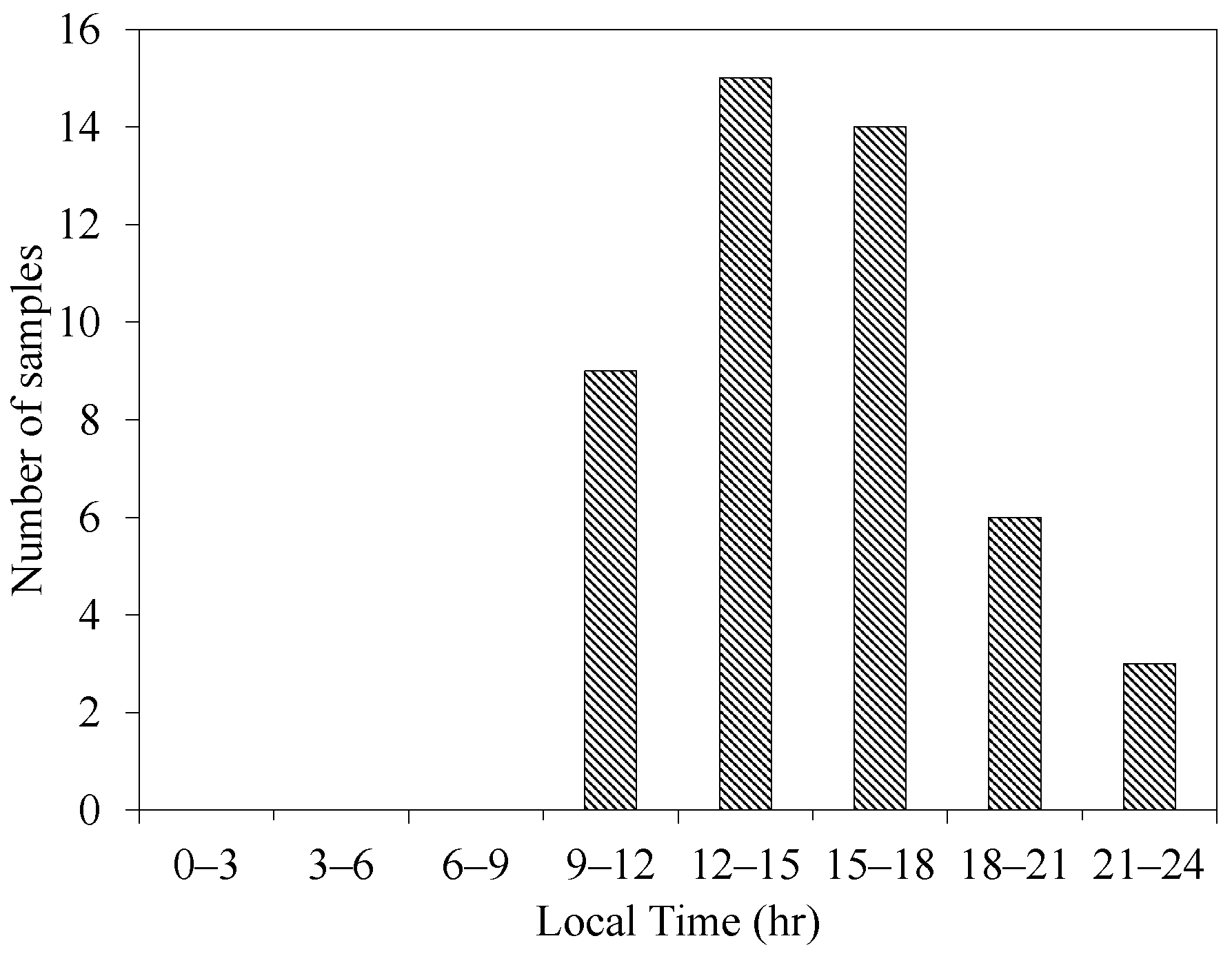
Only 47 samples (30 min each) were involved in the analysis out of the 20-day continuous measurements. The histogram in Figure 2 illustrates the distribution of the considered samples over the day hours. The thermal stability range of the selected samples was within $-1.0\lesssim \zeta \lesssim 0.05$, which can be treated as near-neutral conditions. A 2-Hz low-pass spectrum filter was applied to exclude the noise. The mesoscale motions (large-scale thermally-generated TCS) were filtered out via a high-pass spectrum filter, in which the cut-off frequency was calculated by wavelet analysis, as to be discussed in Section 2.2.

2.1. Scaling

A problem in the analogy between laboratory-scale measurements and atmospheric flows is the difficulty to measure ABL height. The latter is thus either assigned a reasonable value [2,39] or obtained by fitting the site data to the statistical laboratory data [40]. In this research, a method has to be devised to predict the ABL height or to scale ground-normal distances at the minimum. We suggest using the TCS length scale as a scaling parameter for the ABL data. The TCS length scale offers two merits in this context; first, it scales with boundary-layer height, and second, it adapts to flow thermal conditions. The length scale was obtained from wavelet power spectral analysis. The spectrum was expected to exhibit a bimodal distribution, i.e., peaks at two time scales corresponding to the vortex packet and the super-streak. The vortex packet wavelength was implemented in the analysis along with the classical inner scale for the purpose of comparison. We have to stress here that the scaling has no effect on the slopes (As) of the logarithmic relations; it affects only the intercepts (Bs).

2.2. Wavelet Analysis

Wavelet analysis is a mathematical tool for extracting the time traces of certain TCS scales from the measured turbulent signals. The procedure followed in this study was inspired by those in the work of Thomas and Foken [41] and Barthlott et al. [35]. The one-dimensional continuous wavelet coefficient of a function $X(t)$ with respect to a mother wavelet $\psi (t)$ is given by

$$\begin{array}{c}\hfill W_b(a)=\frac{1}{a}{\int }_{-\infty }^{+\infty }X(t)\psi \left(\frac{t-b}{a}\right)dt,\end{array}$$

(7)

where a is the scale, and b is the shift. The Morlet wavelet was applied as the continuous wavelet function. This selection was made on the grounds that the Morlet wavelet is well-localised in the frequency domain. The wavelet scales are related to real time scales D through

$$\begin{array}{c}\hfill D=\frac{a\Delta t\pi }{{\omega }_{peak}},\end{array}$$

(8)

where ${\omega }_{peak}$ is the peak frequency of the wavelet function (5 rad s${}^{-1}$ for the Morlet wavelet). The studied time scales ranged between 8 and 140 s, which covered the expected range of scales of TCS in the atmosphere [42,43]. Only fluctuations greater than 40% of the series maximum value were recognised as TCS [35,43]. To determine the characteristic time scale of the signal, we calculated the wavelet variance as

$$\begin{array}{c}\hfill WV(a)={\int }_{-\infty }^{+\infty }{\left|W_b(a)\right|}^{2}db,\end{array}$$

(9)

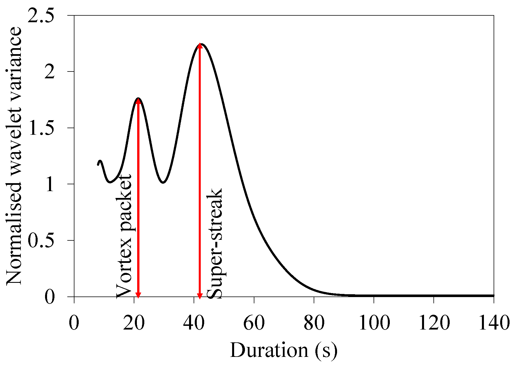
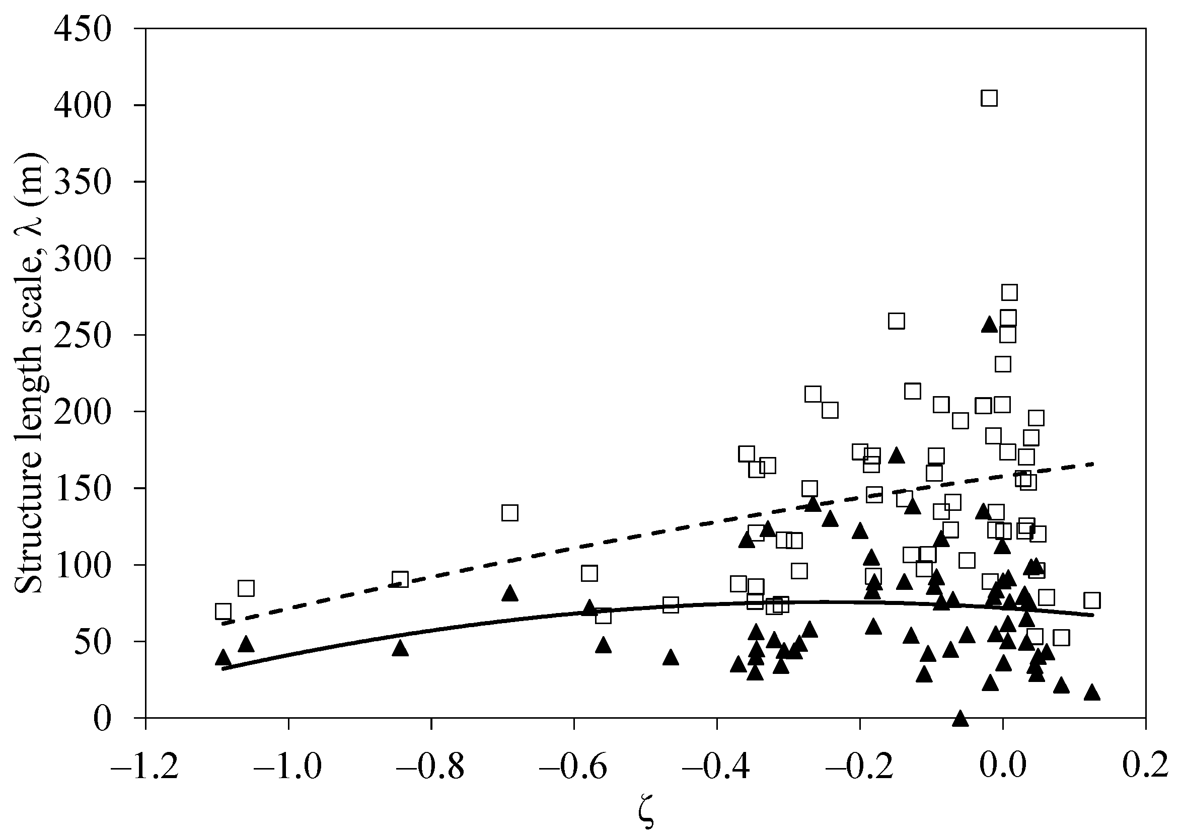
which can be considered equivalent to the Fourier power spectrum. The dominant time scale corresponding to the dominant coherent structure represents the peak wavelet variance. The wavelet analysis was applied to the vertical velocity fluctuation $w^{\prime }$ instead of the streamwise component $u^{\prime }$ because the former is less influenced by mesoscale motions [44,45,46]. The 12.0-m height data were used in the analysis. An example of the resulting spectra is illustrated in Figure 3. Only the highest two peaks were considered, while all other local peaks were ignored. Similar to the two peaks of the Fourier energy spectrum [36], the peak of the shorter time scale was related to the vortex packet whereas that of the longer time scale to the super-streak. The length scale was estimated from Taylor’s frozen turbulence hypothesis by multiplying the time scale by the wind speed. The calculated length scales of the vortex packet and super-streak vary with atmospheric stability, as shown in Figure 4.

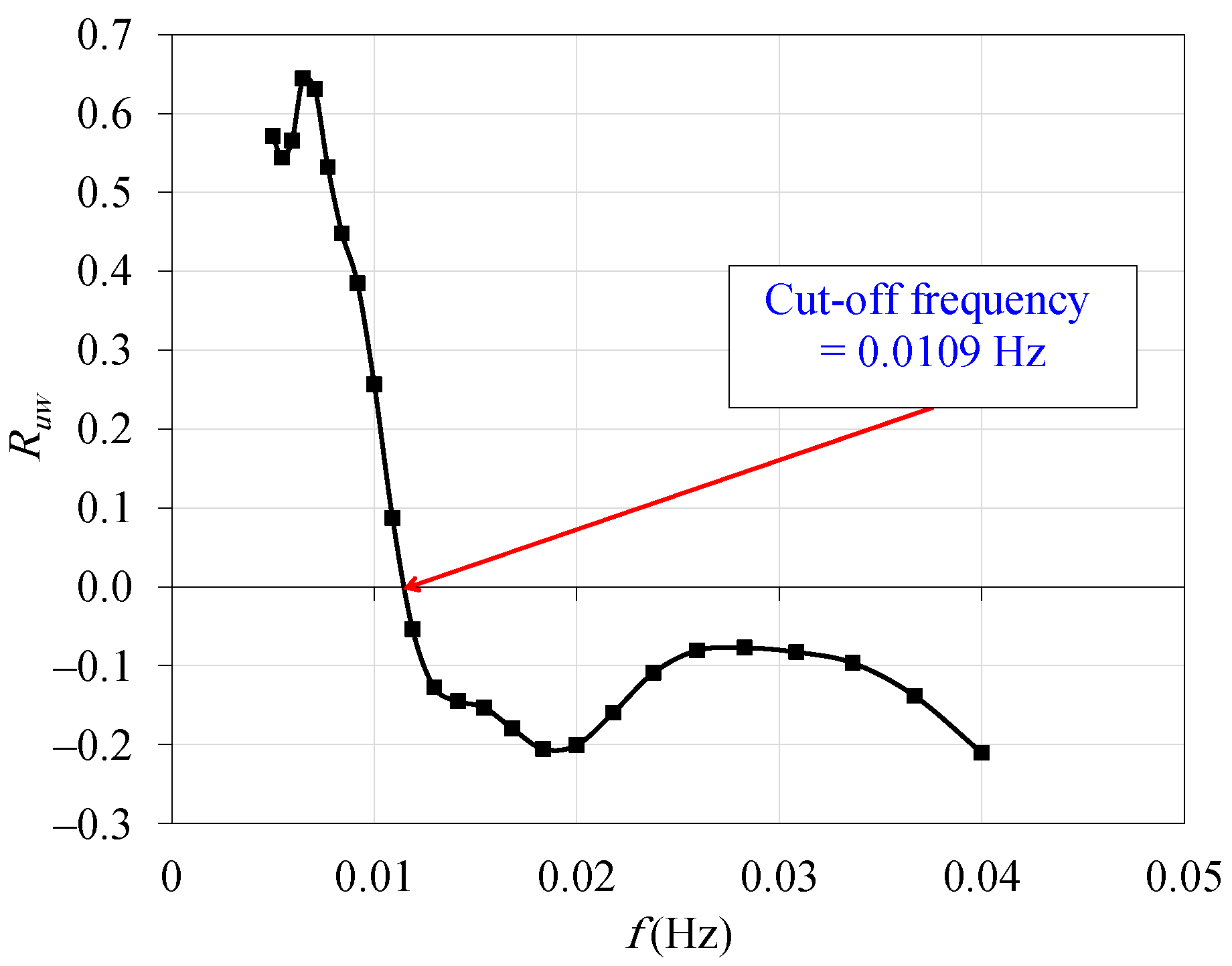
The wavelet analysis was applied to determine the cut-off frequency of the mesoscale motions. Various techniques were applied to remove these scales without harming the low-frequency turbulent motions [34,40]. In this research, a method based on wavelet decomposition was applied. The low frequencies (<0.04 Hz) were decomposed into 25 wavelets. The $u^{\prime }$ signals were cross-correlated with the $w^{\prime }$ signals. An example of the variation of the cross-correlation factor with wavelet frequency is illustrated in Figure 5. A fundamental property of TCS is the negative cross-correlation between $u^{\prime }$ and $w^{\prime }$ [30]. Thus, the cut-off frequency was defined as the border between positive and negative correlations.

3. Results and Discussion

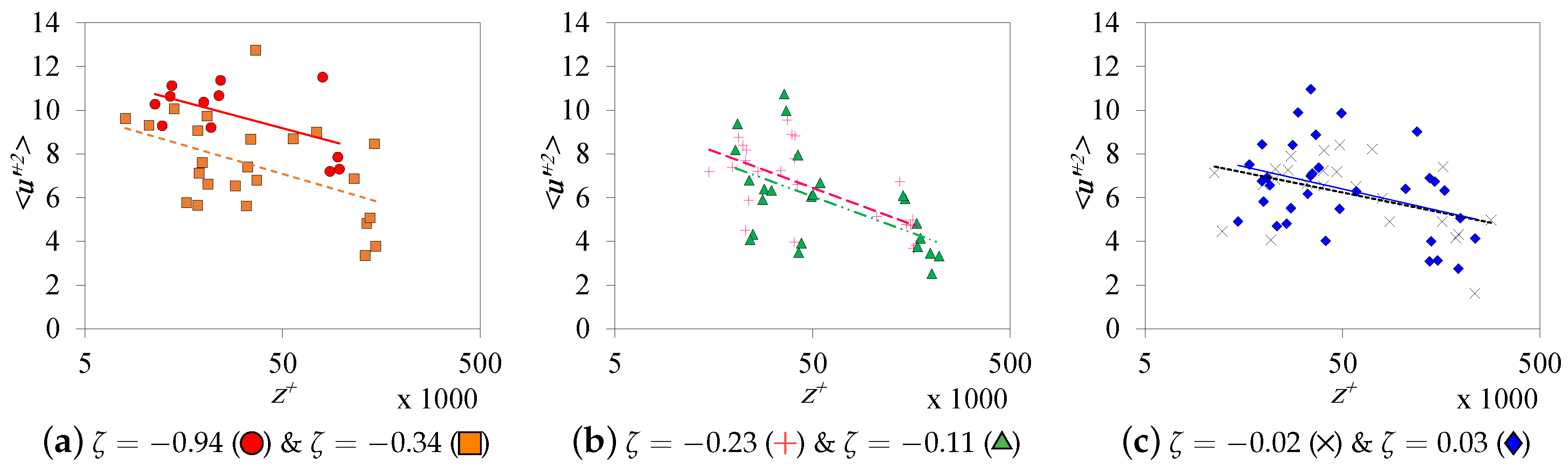
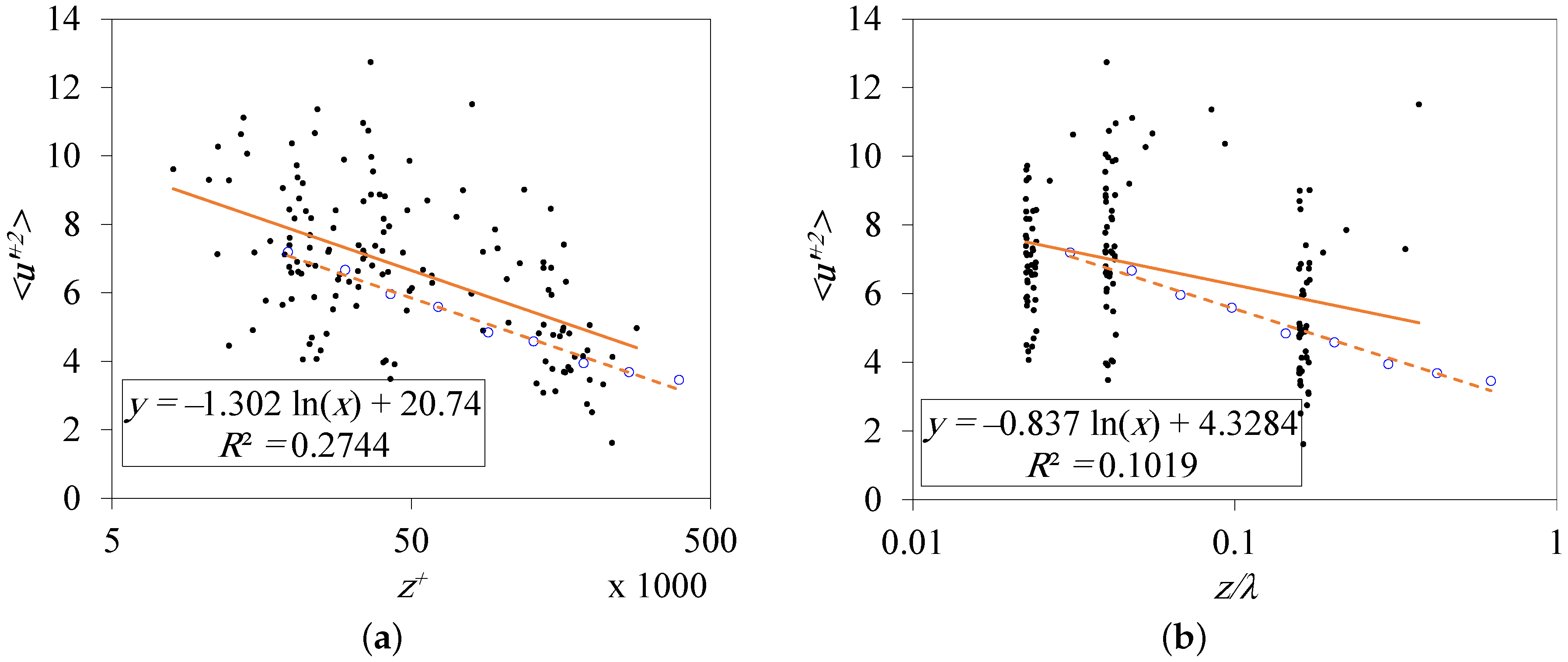
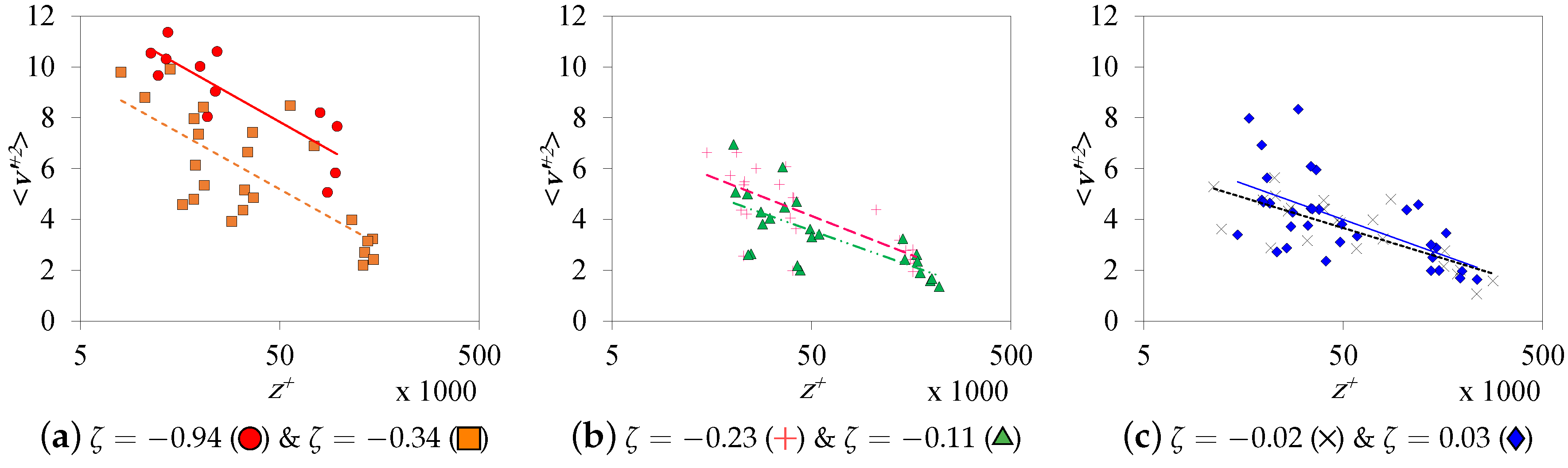
The dataset was subdivided into six subsets according to atmospheric stability. The details of the subsets are listed in

Table 1. Details of data subsets.

No	Source	Nominal $\mathit{\zeta }$ ${}^{†}$	Range of $\mathit{\zeta }$	Number of Samples	Data Symbol	Fitting Line
1	Current research	$-0.94$	$-1.09$ to $-0.69$	12 ${}^{*}$
2	Current research	$-0.34$	$-0.37$ to $-0.31$	24
3	Current research	$-0.23$	$-0.29$ to $-0.18$	24	+
4	Current research	$-0.11$	$-0.15$ to $-0.07$	24
5	Current research	$-0.02$	$-0.06$ to $0.00$	24	×
6	Current research	$0.03$	$0.00$ to $0.05$	33
7	Hutchins et al. [40]	0	$-0.02$ to $0.03$	4	○
8	Kunkel and Marusic [52]	0	∼0	9	∗

[†] Geometric mean; [${}^{*}$] 4 data points × three sensors.

. The logarithmic relations of the windward turbulent velocity variance of the six subsets are illustrated in Figure 6. The majority of the data extend from $z^{+}\simeq$ 8000 to 300,000, which translates into outer-scaling to $0.02\lesssim z/\lambda \lesssim 0.2$. The finding suggests that the data mostly fall in the IS [2]. As illustrated in Figure 6, the current data do not show a clear correlation between the slope of the logarithmic $\langle {u^{\prime +}}^2\rangle$ relation and the atmospheric stability. This finding can be either caused by the ever-lasting effect of the mesoscale motions or some universality of the Townsend–Perry constant. Thereby, the logarithmic relation is obtained as an average for the whole $47\times 3$ samples, as shown in Figure 7. The average slope of the near-neutral atmospheric data is $-1.302$ (inner-scaled) or $-0.837$ (outer-scaled), which are very close to the values surveyed in the literature [2,47,48]. While Diwan and Morrison [49], among others, expected $A_u$ to increase with $R{e}_{*}$ to values higher than 1.243, a survey conducted by Laval et al. [47], which was based on the experiments of Vallikivi et al. [50], reported an inverse relation between $A_u$ and $R{e}_{*}$ indicating that values lower than 1.16 are possible at high $R{e}_{*}$.

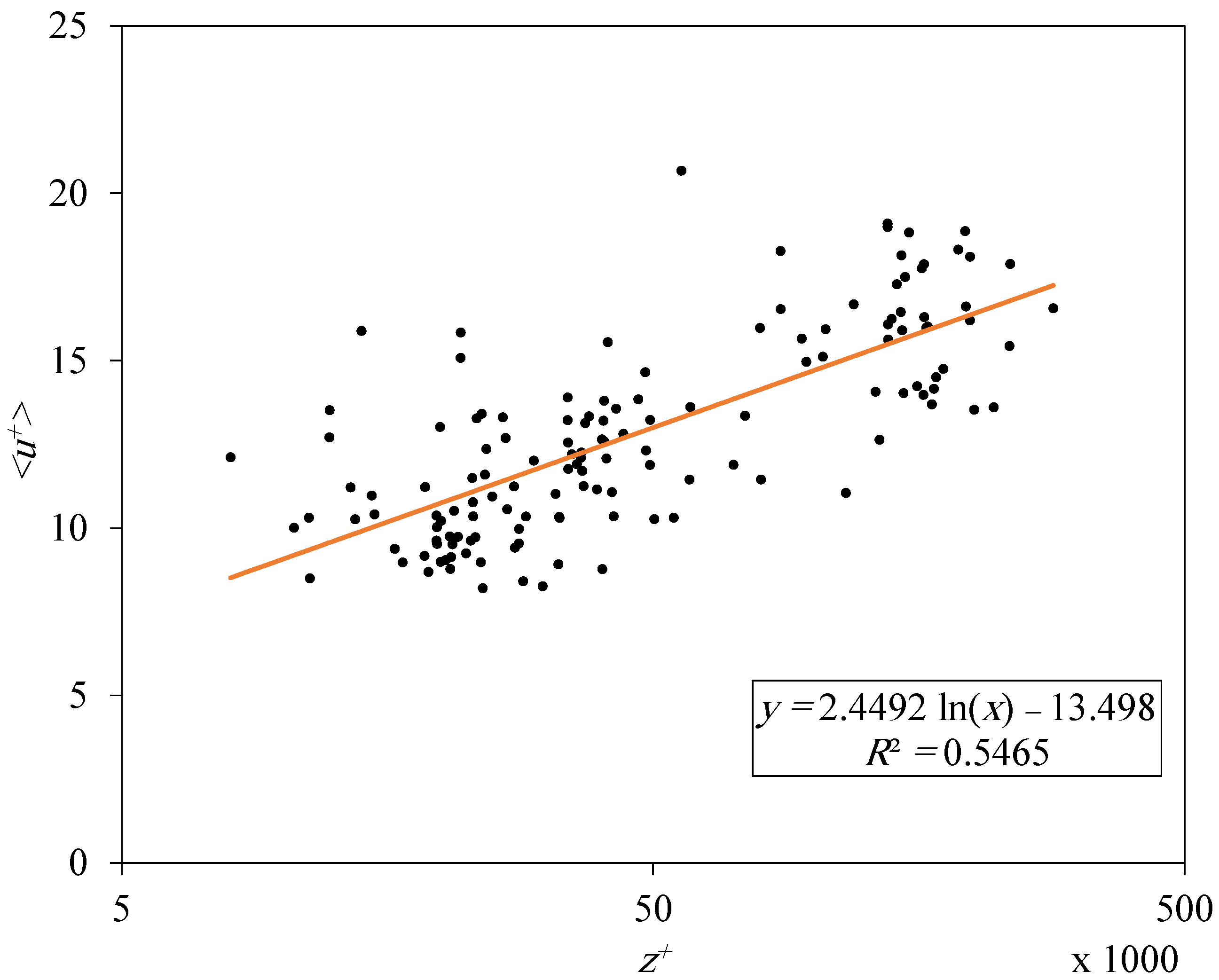
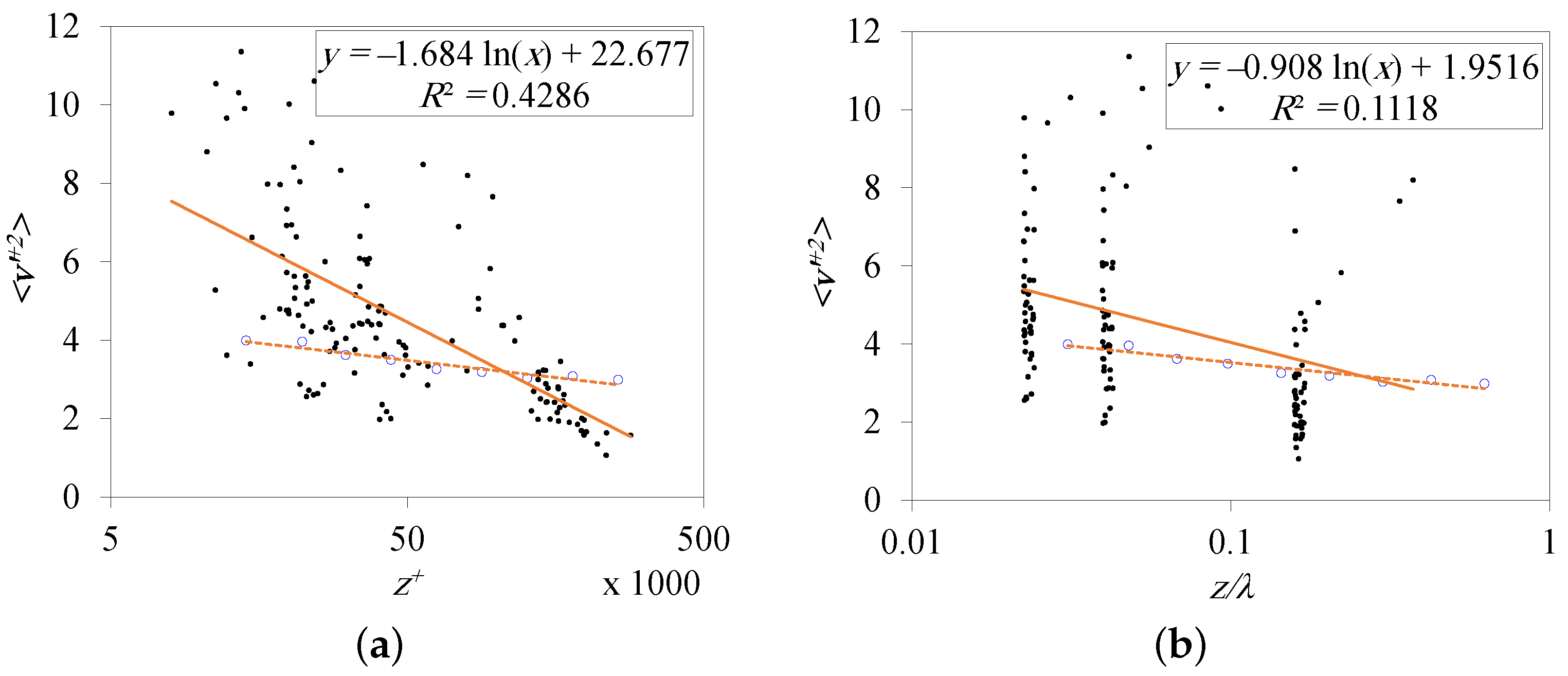
Similarly, an average fitting for the near-neutral atmospheric mean velocity data was plotted in Figure 8. These operations yield a slope of ∼2.5, which corresponds to $\kappa =0.41$, but the intercept is larger compared with the commonly acceptable value (5.0) due to the surface roughness effect [51]. A much definite trend can be found in $\langle {v^{\prime +}}^2\rangle$ logarithmic relations, as shown in Figure 9. The slope of the relation increases as the atmosphere becomes more convective and reaches a high value of 1.92 in the $\zeta =-0.94$ subset. The slope is at the minimum at $\zeta \sim 0$ with a value of 1.038. The average slope is $-1.684$ for the inner-scaled data (Figure 10a) and $-0.908$ for the $\lambda$-scaled data (Figure 10b). The deviation from the results obtained by Hutchins et al. [40] is obvious.

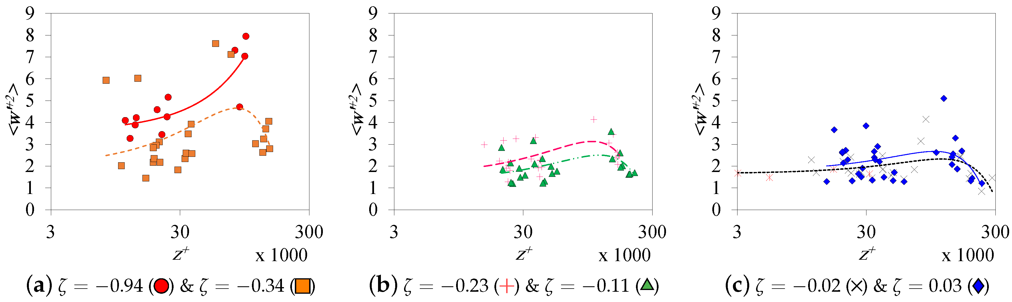
According to Townsend’s expectations, $\langle {w^{\prime +}}^2\rangle$ exhibits a constant value with height. This scenario is true up to a certain level above ground, as demonstrated in Figure 11. At the higher altitudes, the variance peaks and then decays again. The peak dampens while approaching the $\zeta =0$ condition. Moreover, the constant-$\langle {w^{\prime +}}^2\rangle$ zone is thickest in neutral atmosphere and erodes away from it. The data are best fit with polynomial second-order trend lines. The constant value of $\langle {w^{\prime +}}^2\rangle$ in the neutral subset is 1.656, which coincides with the data of Kunkel and Marusic [52] and the values in the ABL literature, for example, References [24,27,28].

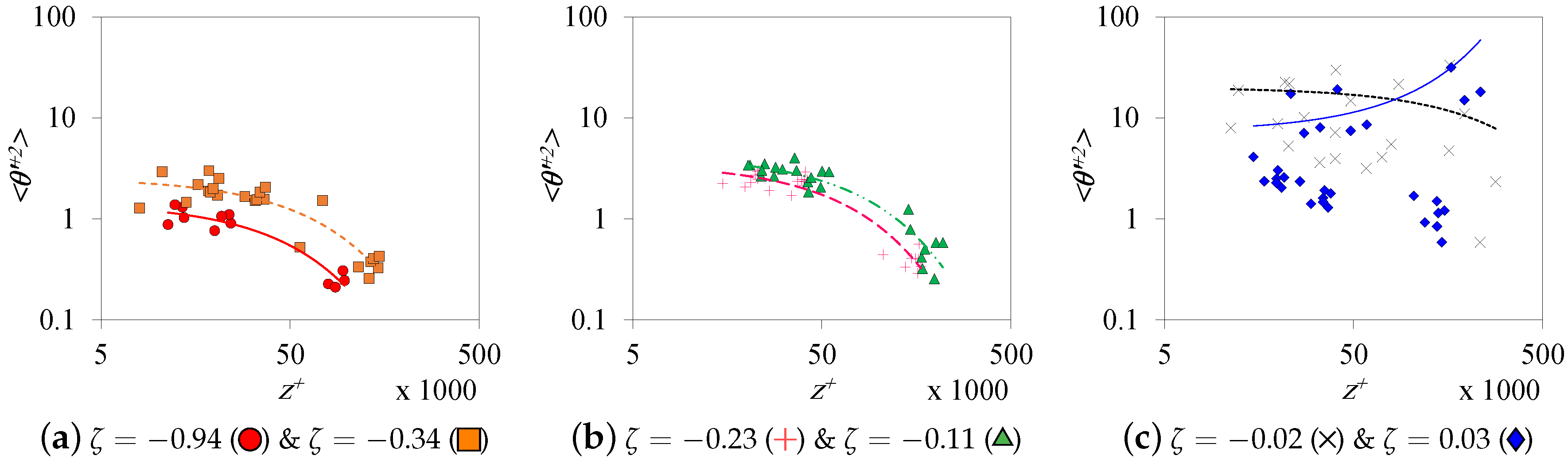
The temperature variance $\langle {{\theta }^{\prime +}}^2\rangle$ follows an exponential trend (Figure 12), specially at high convective conditions ($\zeta <-0.11$). As a matter of fact, temperature fluctuations weaken away from the ground under convective conditions and strengthen under stable conditions with the neutral state witnessing null variation with height. The turbulent temperature variance tends at ground-level to a value ranging between 1.44 and 20, according to $\zeta$. Despite that the power regression is more common in the literature [24,28], the second-order polynomial regression for $\langle {w^{\prime +}}^2\rangle$ and the exponential regression for $\langle {{\theta }^{\prime +}}^2\rangle$ were found to best-fit the current data. Recall that this is the first time using $z^{+}$ as a height scale instead of the typical $\zeta$ and $z/\delta$.

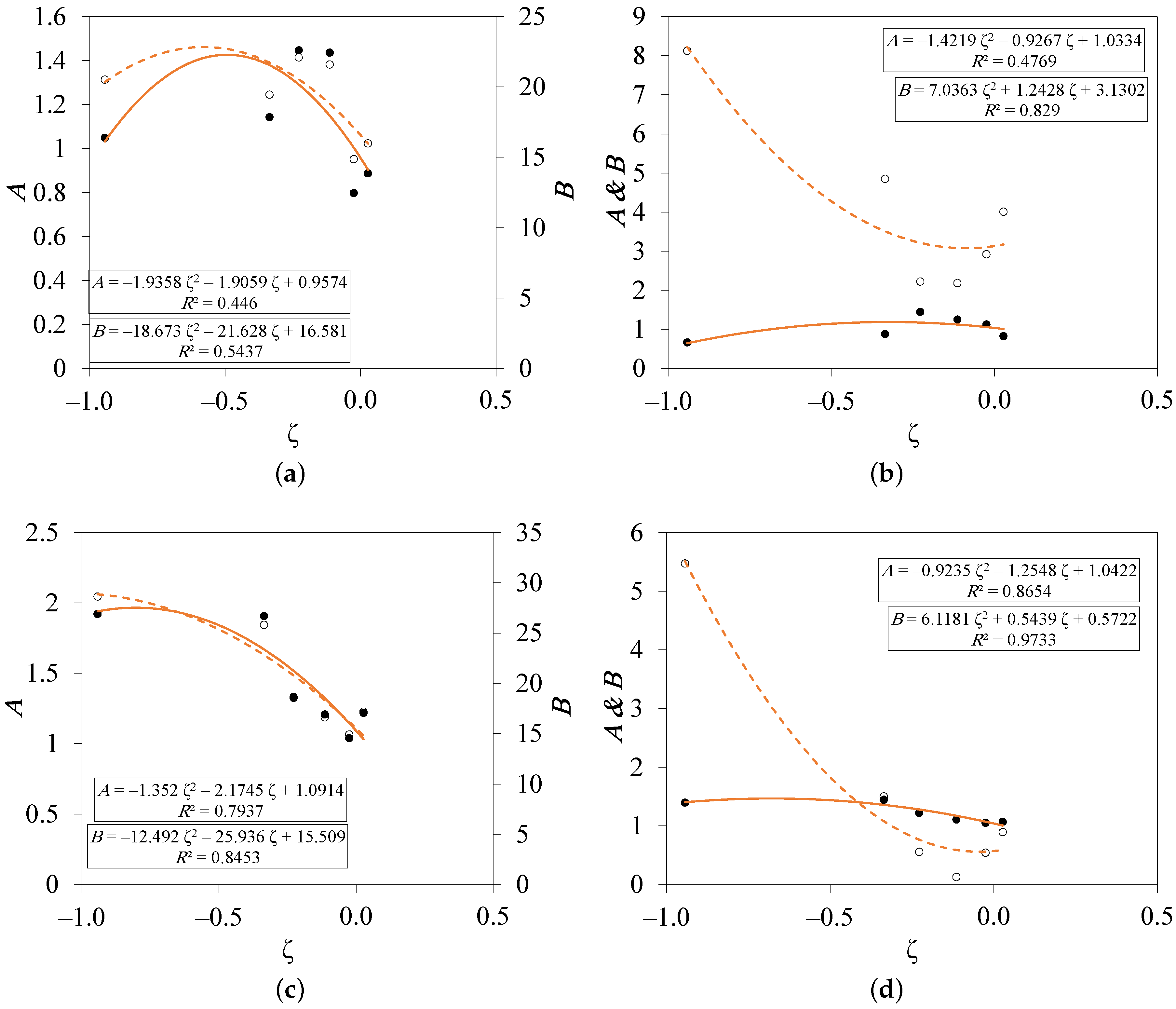
We are now to quantify the effect of atmospheric thermal condition on the “logarithmic” turbulent correlations. Figure 13 shows the effect of $\zeta$ on the slope (A) and intercept (B) of the logarithmic $\langle {u^{\prime +}}^2\rangle$ and $\langle {v^{\prime +}}^2\rangle$ relations. Regarding $\langle {u^{\prime +}}^2\rangle$, the current data do not show a clear impact for the atmospheric condition on the Townsend–Perry constant (A). The value of the constant ranges between 0.8 and 1.45 for inner-scaled correlations and between 0.66 and 1.44 for outer-scaled correlations. Unlike the case with windward correlations, the atmospheric stability effect on crosswind correlations is obvious. The slope varies from 1.04/1.05 at $\zeta \simeq 0$ to 1.92/1.4 at $\zeta \simeq -0.94$ for inner-/outer-scaled correlations. More investigations under wider atmospheric stability ranges are needed to confirm this conclusion. The value of B increases in convective stability condition for $\langle {u^{\prime +}}^2\rangle$ and $\langle {v^{\prime +}}^2\rangle$.

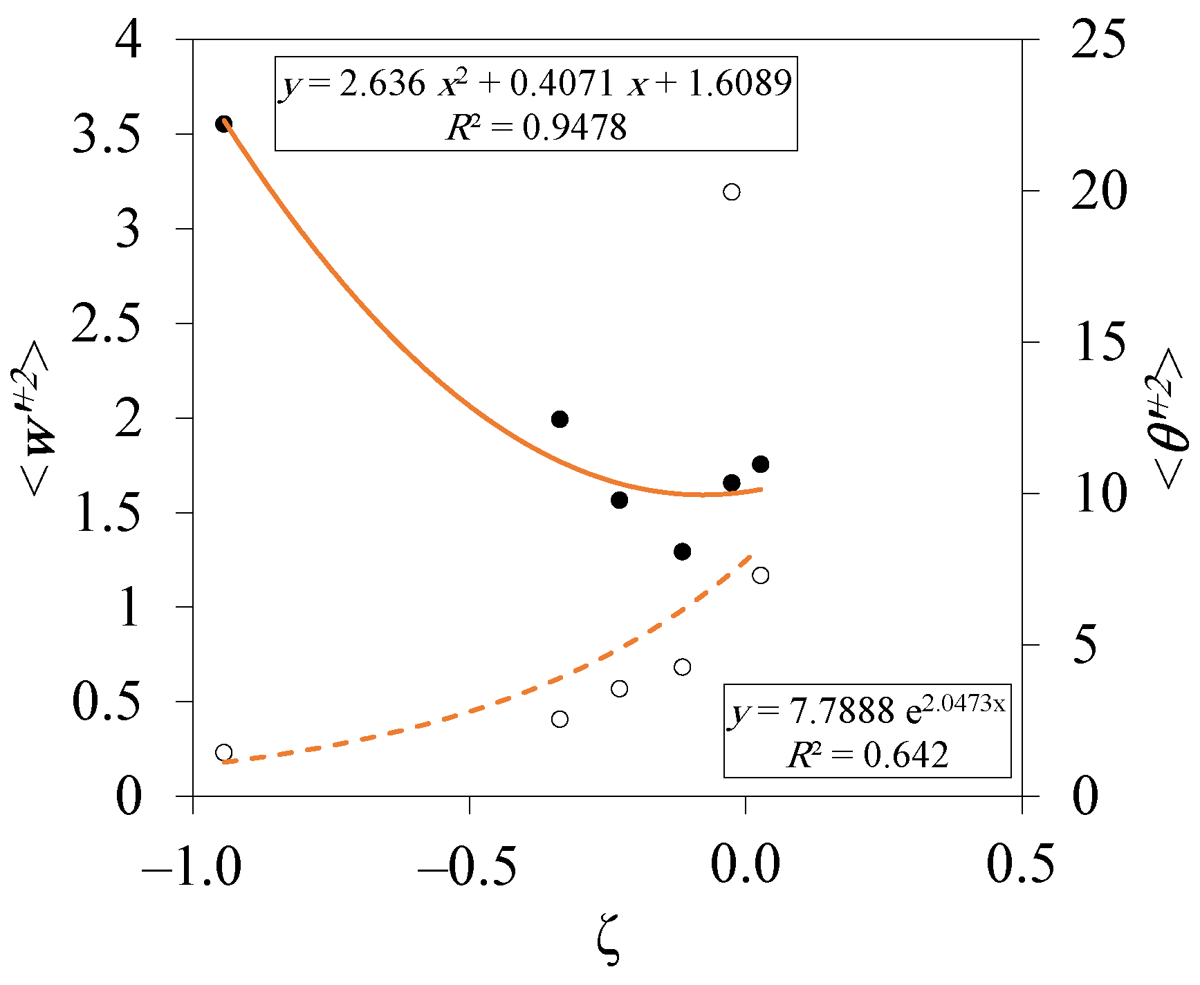
The correlations of $\langle {w^{\prime +}}^2\rangle$ and $\langle {{\theta }^{\prime +}}^2\rangle$ for the different atmospheric subsets are given in

Table 2. Correlations of the variances of the turbulent vertical velocity and temperature with ground-normal distance ($z^{+}$) under different stability conditions.

Stability Range	$\langle {{\mathit{w}}^{\prime +}}^2\rangle$	$\langle {{\mathit{\theta }}^{\prime +}}^2\rangle$
$-1.09$ to $-0.69$	$7\times {10}^{-11}{z^{+}}^2+3\times {10}^{-5}{z}^{+}+3.5534$	$1.4404e^{-2\times {10}^{-5}{z}^{+}}$
	$R^2=0.7255$	$R^2=0.9136$
$-0.37$ to $-0.31$	$-4\times {10}^{-10}{z^{+}}^2+6\times {10}^{-5}{z}^{+}+1.9922$	$2.5488e^{-1\times {10}^{-5}{z}^{+}}$
	$R^2=0.1106$	$R^2=0.8364$
$-0.29$ to $-0.18$	$-1\times {10}^{-10}{z^{+}}^2+3\times {10}^{-5}{z}^{+}+1.5649$	$3.5555e^{-1\times {10}^{-5}{z}^{+}}$
	$R^2=0.1725$	$R^2=0.9237$
$-0.15$ to $-0.07$	$-9\times {10}^{-11}{z^{+}}^2+2\times {10}^{-5}{z}^{+}+1.2926$	$4.2686e^{-1\times {10}^{-5}{z}^{+}}$
	$R^2=0.1485$	$R^2=0.8932$
$-0.06$ to $0.00$	$-5\times {10}^{-11}{z^{+}}^2+1\times {10}^{-5}{z}^{+}+1.656$
	$R^2=0.1948$
$0.00$ to $0.05$	$-9\times {10}^{-11}{z^{+}}^2+2\times {10}^{-5}{z}^{+}+1.7552$
	$R^2=0.1156$

. Except for highly convective conditions ($\zeta \le -0.69$), the vertical wind variance is weakly correlated with height, i.e., the $R^2$ values of the proposed best-fit relationships are less than $0.2$. Regarding the temperature variance, the proposed correlations closely describe the experimental data, as suggested by the $R^2$ values. This is true under all convective atmospheric conditions ($\zeta \le -0.07$), whereas under the neutral conditions, there is no clear trend for the temperature variance with height. Figure 14 presents the second-order polynomial and the exponential fittings for the ground-level values of $\langle {w^{\prime +}}^2\rangle$ ($B_w$) and $\langle {{\theta }^{\prime +}}^2\rangle$. The variances have ground values of 1.6089 and 7.7888 in neutral atmosphere, which are in good agreement with those in the literature. The convective condition creates higher ground-level values of $\langle {w^{\prime +}}^2\rangle$ and lower of $\langle {{\theta }^{\prime +}}^2\rangle$ due to the decay of mechanical turbulence ($u_{*}$) and growth of thermal currents ($\overline{w^{\prime }{\theta }^{\prime }}$). A comparison between the $\zeta \sim 0$ values of all correlation constants in the current research and those in the literature is listed in

Table 3. Slopes (As) and intercepts (Bs) of the logarithmic correlations of the mean velocity ($\langle u^{+}\rangle$) and turbulent fluctuation variances ($\langle {u^{\prime +}}^2\rangle$, $\langle {v^{\prime +}}^2\rangle$, $\langle {w^{\prime +}}^2\rangle$ and $\langle {{\theta }^{\prime +}}^2\rangle$) under the neutral atmospheric condition.

Relation	Source	Notes	Scale	Parameter
$\langle u^{+}\rangle$	Current research	as an average for the whole dataset, Figure 8	$\nu /u_{*}$	$A=2.45$
				$B=-13.5$
				$\kappa =0.408$
	Marusic et al. [2]		$\nu /u_{*}$	$A=2.44$∼2.60
				$B=4.44$
				$\kappa =0.410$
$\langle {u^{\prime +}}^2\rangle$	Current research	as an average for the whole dataset, Figure 7a	$\nu /u_{*}$	$A=1.302$
				$B=20.74$
	Hutchins et al. [40]		$\nu /u_{*}$	$A=1.299$
				$B=19.913$
	Current research	as an average for the whole dataset, Figure 7b	$\lambda$	$A=0.837$
				$B=4.3284$
	Marusic et al. [2]		$\delta$	$A=1.33$
				$B=2.14$
$\langle {v^{\prime +}}^2\rangle$	Current research	from second-order polynomial interpolation, Figure 13c	$\nu /u_{*}$	$A=1.0914$
				$B=15.509$
	Hutchins et al. [40]		$\nu /u_{*}$	$A=0.381$
				$B=7.6028$
	Current research	from second-order polynomial interpolation, Figure 13d	$\lambda$	$A=1.0422$
				$B=0.5722$
	Hutchins et al. [40]		$\delta$	$A=0.365$
				$B=2.688$
$\langle {w^{\prime +}}^2\rangle$${}^{†}$	Current research	from second-order polynomial interpolation for ground-level values, Figure 14	$\nu /u_{*}$	$B=1.6089$
	Kunkel and Marusic [52]		$\nu /u_{*}$	$B=1.676$
$\langle {{\theta }^{\prime +}}^2\rangle$${}^{†}$	Current research	from exponential interpolation for ground-level values, Figure 14	$\nu /u_{*}$	$7.7888$
	Pahlow et al. [24], Nieuwstadt [28]		$\nu /u_{*}$	$9.0$

[†] ground-normal values.

. Except for $\langle {v^{\prime +}}^2\rangle$, the values generally coincide.

4. Conclusions

This analysis validates Townsend’s theory in high Reynolds-number atmospheric flow under different stability conditions. The analyses were applied to open flow coastal data in three heights, namely, 1.7, 3.0, and 12.0 m. After enforcing the rigorous screening rules, only 47 × 3 samples between $\zeta \simeq -1.1$ and $0.05$ were available for analysis. Two approaches were used to scale the boundary layer parameters, namely, the inner scale ($\nu /u_{*}$) and the outer scale ($\lambda$), which resembles the TCS wavelength calculated by wavelet spectral analysis. The following conclusions can be drawn from the results:

• The Townsend–Perry constant for the windward velocity variance is not a function of thermal stability in the studied range of atmospheric conditions. An average value for the current dataset is 1.302, which is consistent with those in other atmospheric studies [2].
• The slope of the crosswind correlation clearly decreases in the positive stability direction. The values range between 1 and 2 for the current dataset.
• The intercept (B) of all relations increases in the convective atmosphere direction.
• The variances of the vertical velocity and temperature were best-fit by second-order polynomial and exponential regressions, respectively.
• The variance of the vertical velocity manifests a local peak at high altitudes and approaches asymptotic values at the ground level. The peak dampens and the asymptotic value decreases close to the neutral atmospheric condition. A ground-level (zero-$\zeta$) value of 1.6089 was recorded in this research.
• The temperature variance varies exponentially with $z^{+}$, particularly at $\zeta \lesssim -0.11$. The fluctuations strengthen with height under stable conditions and dampen with height under convective conditions. The ground-level value in neutral atmosphere is 7.7888.

The current results pave the way to the solid modelling of turbulent statistics in the atmospheric IS. However, further research is needed to support the conclusions and widen the scope of analyses to all the applicable atmospheric range.

References

- Nagib, H.M.; Chauhan, K.A. Variations of von Kármán coefficient in canonical flows. Phys. Fluids 2008, 20, 101518. [Google Scholar] [CrossRef]
- Marusic, I.; Monty, J.P.; Hultmark, M.; Smits, A.J. On the logarithmic region in wall turbulence. J. Fluid Mech. 2013, 716, R3. [Google Scholar] [CrossRef] [Green Version]
- Miguntanna, N.S.; Moses, H.; Sivakumar, M.; Yang, S.Q.; Enever, K.J.; Riaz, M.Z.B. Re-examining log law velocity profile in smooth open channel flows. Environ. Fluid Mech. 2020, 20, 953–986. [Google Scholar] [CrossRef]
- Townsend, A. The Structure of Turbulent Shear Flow; Cambridge Monographs on Mechanics, Cambridge University Press: Cambridge, UK, 1976. [Google Scholar]
- Townsend, A. Equilibrium layers and wall turbulence. J. Fluid Mech. 1961, 11, 97–120. [Google Scholar] [CrossRef]
- Nickels, T.; Marusic, I.; Hafez, S.; Hutchins, N.; Chong, M. Some predictions of the attached eddy model for a high Reynolds number boundary layer. Philos. Trans. R. Soc. Lond. A Math. Phys. Eng. Sci. 2007, 365, 807–822. [Google Scholar] [CrossRef] [Green Version]
- Head, M.; Bandyopadhyay, P. New aspects of turbulent boundary-layer structure. J. Fluid Mech. 1981, 107, 297–338. [Google Scholar] [CrossRef]
- Perry, A.; Chong, M. On the mechanism of wall turbulence. J. Fluid Mech. 1982, 119, 173–217. [Google Scholar] [CrossRef] [Green Version]
- Perry, A.; Henbest, S.; Chong, M. A theoretical and experimental study of wall turbulence. J. Fluid Mech. 1986, 165, 163–199. [Google Scholar] [CrossRef] [Green Version]
- Marusic, I. On the role of large-scale structures in wall turbulence. Phys. Fluids 2001, 13, 735–743. [Google Scholar] [CrossRef] [Green Version]
- Adrian, R.; Meinhart, C.; Tomkins, C. Vortex organization in the outer region of the turbulent boundary layer. J. Fluid Mech. 2000, 422, 1–54. [Google Scholar] [CrossRef] [Green Version]
- Zhou, J.; Adrian, R.J.; Balachandar, S.; Kendall, T. Mechanisms for generating coherent packets of hairpin vortices in channel flow. J. Fluid Mech. 1999, 387, 353–396. [Google Scholar] [CrossRef]
- Dennis, D.J.; Nickels, T.B. Experimental measurement of large-scale three-dimensional structures in a turbulent boundary layer. Part 1. Vortex packets. J. Fluid Mech. 2011, 673, 180–217. [Google Scholar] [CrossRef]
- Woodcock, J.; Marusic, I. The Attached Eddy Hypothesis and von Kármán’s Constant. Dynamics 2014, 7, 8. [Google Scholar]
- Hwang, Y. Statistical structure of self-sustaining attached eddies in turbulent channel flow. J. Fluid Mech. 2015, 767, 254–289. [Google Scholar] [CrossRef] [Green Version]
- Hwang, Y.; Cossu, C. Self-sustained process at large scales in turbulent channel flow. Phys. Rev. Lett. 2010, 105, 044505. [Google Scholar] [CrossRef] [PubMed] [Green Version]
- Cossu, C.; Hwang, Y. Self-sustaining processes at all scales in wall-bounded turbulent shear flows. Philos. Trans. R. Soc. A 2017, 375, 20160088. [Google Scholar] [CrossRef] [PubMed]
- Hultmark, M. A theory for the streamwise turbulent fluctuations in high Reynolds number pipe flow. J. Fluid Mech. 2012, 707, 575–584. [Google Scholar] [CrossRef] [Green Version]
- Harun, Z.; Ghopa, W.A.W.; Abdullah, S.; Ghazali, M.I.; Abbas, A.A.; Rasani, M.R.; Zulkifli, R.; Wan Mahmood, W.; Mansor, M.R.A.; Abidin, Z.Z.; et al. The development of a multi-purpose wind tunnel. J. Teknol. 2016, 10, 63–70. [Google Scholar] [CrossRef] [Green Version]
- Meneveau, C.; Marusic, I. Generalized logarithmic law for high-order moments in turbulent boundary layers. J. Fluid Mech. 2013, 719, R1. [Google Scholar] [CrossRef] [Green Version]
- Monin, A.S.; Obukhov, A.M. Osnovnye zakonomernosti turbulentnogo peremesivanija v prizemnom sloe atmosfery (Basic Laws of Turbulent Mixing in the Atmosphere Near the Ground). Tr. Geofiz. Inst. SSSR 1954, 24, 163–187. [Google Scholar]
- Dyer, A. A review of flux-profile relationships. Bound.-Layer Meteorol. 1974, 7, 363–372. [Google Scholar] [CrossRef]
- Lotfy, E.R.; Harun, Z. Effect of atmospheric boundary layer stability on the inclination angle of turbulence coherent structures. Environ. Fluid Mech. 2017, 18, 637–659. [Google Scholar] [CrossRef]
- Pahlow, M.; Parlange, M.B.; Porté-Agel, F. On Monin–Obukhov similarity in the stable atmospheric boundary layer. Bound.-Layer Meteorol. 2001, 99, 225–248. [Google Scholar] [CrossRef] [Green Version]
- Kader, B.; Yaglom, A. Mean fields and fluctuation moments in unstably stratified turbulent boundary layers. J. Fluid Mech. 1990, 212, 637–662. [Google Scholar] [CrossRef]
- Emeis, S. Surface-Based Remote Sensing of the Atmospheric Boundary Layer; Springer Science & Business Media: Berlin/Heidelberg, Germany, 2010; Volume 40. [Google Scholar]
- Nieuwstadt, F. Some aspects of the turbulent stable boundary layer. In Boundary Layer Structure; Springer: Berlin/Heidelberg, Germany, 1984; pp. 31–55. [Google Scholar]
- Nieuwstadt, F.T. The turbulent structure of the stable, nocturnal boundary layer. J. Atmos. Sci. 1984, 41, 2202–2216. [Google Scholar] [CrossRef]
- Harun, Z.; Lotfy, E.R. Generation, Evolution, and Characterization of Turbulence Coherent Structures. In Turbulence and Related Phenomena; IntechOpen: London, UK, 2018. [Google Scholar]
- Adrian, R.J. Hairpin vortex organization in wall turbulence a. Phys. Fluids 2007, 19, 041301. [Google Scholar] [CrossRef] [Green Version]
- Dennis, D.J.; Nickels, T.B. Experimental measurement of large-scale three-dimensional structures in a turbulent boundary layer. Part 2. Long structures. J. Fluid Mech. 2011, 673, 218–244. [Google Scholar] [CrossRef]
- Lotfy, E.R.; Abbas, A.A.; Zaki, S.A.; Harun, Z. Characteristics of Turbulent Coherent Structures in Atmospheric Flow Under Different Shear–Buoyancy Conditions. Bound.-Layer Meteorol. 2019, 173, 115–141. [Google Scholar] [CrossRef]
- Chauhan, K.; Hutchins, N.; Monty, J.; Marusic, I. Structure inclination angles in the convective atmospheric surface layer. Bound.-Layer Meteorol. 2013, 147, 41–50. [Google Scholar] [CrossRef]
- Thomas, C.; Foken, T. Organised motion in a tall spruce canopy: Temporal scales, structure spacing and terrain effects. Bound.-Layer Meteorol. 2007, 122, 123–147. [Google Scholar] [CrossRef]
- Barthlott, C.; Drobinski, P.; Fesquet, C.; Dubos, T.; Pietras, C. Long-term study of coherent structures in the atmospheric surface layer. Bound.-Layer Meteorol. 2007, 125, 1–24. [Google Scholar] [CrossRef]
- Kim, K.; Adrian, R. Very large-scale motion in the outer layer. Phys. Fluids 1999, 11, 417–422. [Google Scholar] [CrossRef]
- Högström, U.; Smedman, A.S. Accuracy of sonic anemometers: Laminar wind-tunnel calibrations compared to atmospheric in situ calibrations against a reference instrument. Bound.-Layer Meteorol. 2004, 111, 33–54. [Google Scholar] [CrossRef]
- Larsén, X.; Smedman, A.S.; Högström, U. Air–sea exchange of sensible heat over the Baltic Sea. Q. J. R. Meteorol. Soc. 2004, 130, 519–539. [Google Scholar] [CrossRef]
- Hommema, S.E.; Adrian, R.J. Packet structure of surface eddies in the atmospheric boundary layer. Bound.-Layer Meteorol. 2003, 106, 147–170. [Google Scholar] [CrossRef]
- Hutchins, N.; Chauhan, K.; Marusic, I.; Monty, J.; Klewicki, J. Towards reconciling the large-scale structure of turbulent boundary layers in the atmosphere and laboratory. Bound.-Layer Meteorol. 2012, 145, 273–306. [Google Scholar] [CrossRef]
- Thomas, C.; Foken, T. Detection of long-term coherent exchange over spruce forest using wavelet analysis. Theor. Appl. Clim. 2005, 80, 91–104. [Google Scholar] [CrossRef]
- Júnior, C.D.; Sá, L.; Pachêco, V.; de Souza, C. Coherent structures detected in the unstable atmospheric surface layer above the Amazon forest. J. Wind Eng. Ind. Aerodyn. 2013, 115, 1–8. [Google Scholar] [CrossRef]
- Starkenburg, D.; Fochesatto, G.J.; Prakash, A.; Cristóbal, J.; Gens, R.; Kane, D.L. The role of coherent flow structures in the sensible heat fluxes of an Alaskan boreal forest. J. Geophys. Res. Atmos. 2013, 118, 8140–8155. [Google Scholar] [CrossRef]
- Vickers, D.; Mahrt, L. Observations of the cross-wind velocity variance in the stable boundary layer. Environ. Fluid Mech. 2007, 7, 55–71. [Google Scholar] [CrossRef]
- Mahrt, L. Characteristics of submeso winds in the stable boundary layer. Bound.-Layer Meteorol. 2009, 130, 1–14. [Google Scholar] [CrossRef] [Green Version]
- Lotfy, E.R.; Zaki, S.A.; Harun, Z. Modulation of the atmospheric turbulence coherent structures by mesoscale motions. J. Braz. Soc. Mech. Sci. Eng. 2018, 40, 178. [Google Scholar] [CrossRef]
- Laval, J.P.; Vassilicos, J.C.; Foucaut, J.M.; Stanislas, M. Comparison of turbulence profiles in high-Reynolds-number turbulent boundary layers and validation of a predictive model. J. Fluid Mech. 2017, 814, R2. [Google Scholar] [CrossRef] [Green Version]
- Carlier, J.; Stanislas, M. Experimental study of eddy structures in a turbulent boundary layer using particle image velocimetry. J. Fluid Mech. 2005, 535, 143–188. [Google Scholar] [CrossRef]
- Diwan, S.S.; Morrison, J.F. Intermediate Scaling and Logarithmic Invariance in Turbulent Pipe Flow. arXiv 2019, arXiv:1909.11951. [Google Scholar]
- Vallikivi, M.; Ganapathisubramani, B.; Smits, A.J. Spectral scaling in boundary layers and pipes at very high Reynolds numbers. J. Fluid Mech. 2015, 771, 303–326. [Google Scholar] [CrossRef]
- Sultan, T.; Ahmad, S.; Cho, J. Numerical study of the effects of surface roughness on water disinfection UV reactor. Chemosphere 2016, 148, 108–117. [Google Scholar] [CrossRef]
- Kunkel, G.J.; Marusic, I. Study of the near-wall-turbulent region of the high-Reynolds-number boundary layer using an atmospheric flow. J. Fluid Mech. 2006, 548, 375–402. [Google Scholar] [CrossRef] [Green Version]
Figure 1.
Example of logarithmic relations in a wind tunnel boundary layer. ◯ refers to the mean velocity profile (left axis), and ⯅ refers to turbulence intensity (right axis). The lines are logarithmic fittings. Flat plate wind-tunnel data ().
Figure 2.
The distribution of the selected samples over the day hours.
Figure 3.
Example of wavelet variance (spectrum), . Values were normalised by the arithmetic mean of the series.
Figure 4.
Variation of the calculated turbulent coherent structures (TCS) length scales () with atmospheric stability; ⯅, vortex packet; □, super-streak. The solid and dashed lines are the second-order polynomial fittings for the two series.
Figure 5.
Variation of the cross-correlation factor between and wavelets with signal frequency. Data were captured at 12.0-m height and .
Figure 6.
Change in turbulent windward velocity variance with stability conditions. The lines are logarithmic fittings for the data. For the chart legend, refer to Table 1.
Figure 7.
Logarithmic relations of the windward velocity variance: (a) inner-scaled, (b) outer-scaled. The small filled circles (•) refer to the current research data, the large open circles (○) refer to [40], and the solid and dashed lines are logarithmic fittings for the two datasets.
Figure 8.
Logarithmic relation of the mean velocity. The small filled circles (•) refer to the current research data, and the solid line is a logarithmic fitting for the current research data.
Figure 9.
Change in turbulent crosswind velocity variance with stability conditions. The lines are logarithmic fittings for the data. For the chart legend, refer to Table 1.
Figure 10.
Logarithmic relations of the crosswind velocity variance: (a) inner-scaled, (b) outer-scaled. The small filled circles (•) refer to the current research data, the large open circles (○) refer to [40], and the solid and dashed lines are logarithmic fittings for the two datasets.
Figure 11.
Change in turbulent ground-normal velocity variance with stability condition. The lines are second-order polynomial fittings for the data. For the chart legend, refer to Table 1.
Figure 12.
Change in turbulent temperature variance with stability condition. The lines are exponential fittings for the data. For the chart legend, refer to Table 1.
Figure 13.
Stability effect on slope (A) and intercept (B) of the logarithmic relations of the windward (a,b) and crosswind (c,d) turbulent velocity fluctuations: (a,c) inner-scaled, (b,d) outer-scaled. • indicates the slope, ⚬ indicates the intercept, and the lines are second-order polynomial fittings.
Figure 14.
Variations in ground-level and values with stability condition. • indicates , ∘ indicates , and the solid and dashed lines are second-order polynomial and exponential fittings for the two series, respectively.