Quantification of Atmospheric Ammonia Concentrations: A Review of Its Measurement and Modeling


Atmospheric Sciences Research Center, State University of New York at Albany, 251 Fuller Road, Albany, NY 12203, USA
*
Author to whom correspondence should be addressed.
Atmosphere 2020, 11(10), 1092; https://doi.org/10.3390/atmos11101092
Submission received: 19 August 2020
/
Revised: 28 September 2020
/
Accepted: 30 September 2020
/
Published: 13 October 2020
(This article belongs to the Section Air Quality)
Abstract
:Ammonia (NH3), the most prevalent alkaline gas in the atmosphere, plays a significant role in PM2.5 formation, atmospheric chemistry, and new particle formation. This paper reviews quantification of [NH3] through measurements, satellite-remote-sensing, and modeling reported in over 500 publications towards synthesizing the current knowledge of [NH3], focusing on spatiotemporal variations, controlling processes, and quantification issues. Most measurements are through regional passive sampler networks. [NH3] hotspots are typically over agricultural regions, such as the Midwest US and the North China Plain, with elevated concentrations reaching monthly averages of 20 and 74 ppbv, respectively. Topographical effects dramatically increase [NH3] over the Indo-Gangetic Plains, North India and San Joaquin Valley, US. Measurements are sparse over oceans, where [NH3] ≈ a few tens of pptv, variations of which can affect aerosol formation. Satellite remote-sensing (AIRS, CrIS, IASI, TANSO-FTS, TES) provides global [NH3] quantification in the column and at the surface since 2002. Modeling is crucial for improving understanding of NH3 chemistry and transport, its spatiotemporal variations, source apportionment, exploring physicochemical mechanisms, and predicting future scenarios. GEOS-Chem (global) and FRAME (UK) models are commonly applied for this. A synergistic approach of measurements↔satellite-inference↔modeling is needed towards improved understanding of atmospheric ammonia, which is of concern from the standpoint of human health and the ecosystem.
Keywords:
review; ammonia; NH3; modeling; measurement; quantification; atmospheric chemistry; particle formation; PM2.51. Introduction
Atmospheric ammonia (NH3), mainly from agriculture with additional sources in industrial and vehicular emissions, plays a key role in many aspects of our environment by virtue of its alkalinity, reactivity, solubility, and abundance. In recent years, there has been an increase in atmospheric ammonia concentrations ([NH3]) mainly due to increased land use for agriculture [1,2,3] to support our burgeoning population. This has generated concern about its negative impacts on the climate and human health. This is especially due to the role of NH3 in the formation of PM2.5 through its neutralization of acidic species in the atmosphere. NH3 has been receiving increasing attention recently due to its potential enhancement of atmospheric new particle formation [4,5]. The impacts of NH3 and the resultant particulate matter on human health [6], ecosystem, and climate deem understanding its concentration in the atmosphere important. NH3 has the following major impacts on the environment. Firstly, NH3 is the greatest contributor to reactive nitrogen deposition [7,8,9,10] in several regions across the globe. Such deposition can contribute to eutrophication of aquatic and terrestrial ecosystems [11,12], which may be enhanced due to the greater bioavailability of NH3 or ammonium (NH4+) compared to other reactive nitrogen species [13,14,15]. Acidification via nitrification, i.e., the conversion of NH3 to nitrite (NO2−) and then to nitrate (NO3−), can also occur [11,12,16,17,18,19,20,21]. For instance, 1 mol of ammonium sulfate ((NH4)2SO4) can potentially release 4 mols of acidity, i.e., H+ ions. Secondly, NH3 can have negative impacts on the ecosystem by direct toxicity, expected above a critical threshold of ∼4 ppbv of [NH3] [22], which is frequently the case in several countries. These impacts can be on vegetation [12,23] through direct damage of stomata, leaves, and other plant surfaces, and biodiversity changes or loss owing to preferential direct uptake of NH3 by certain plant species, as well as affecting plant resilience to abiotic and biotic stressors. Direct impacts on livestock [24,25,26] and humans [27,28] can be through exothermic and alkaline effects on epithelial tissues of the eyes and the respiratory tract. Thirdly, NH3 plays a role in determining the total particle mass and number concentrations, apart from the extent of neutralization of atmospheric particles [4,29,30,31]. The contribution of NH4+ to particulate matter is comparable to that of other inorganic species, such as NO3− and sulfate (SO42−), as seen from modeling [32,33,34] and measurements [9,35,36]. Furthermore, Tsigaridis et al. [33] indicate that the increase in NH4+ absolute (0.13 → 0.37 Tg) and relative (0.5% → 1.3%) contribution to aerosol burden from pre-industrial to present-day times, which is supported by observations from ice core studies [37,38,39]. NH3 also affects the hygroscopicity of particles, an important physicochemical property determining particles’ water carrying capacity. Finally, NH3 can significantly enhance the nucleation rate of aerosol particles through sulfuric acid vapor condensation [4,5,40,41,42], with implications to aerosol indirect radiative forcing. Furthermore, gas-particle partitioning of NH3 to form NH4+ salts can contribute to the continued growth of these newly-formed aerosol particles. Although NH3 shows thermodynamic preference for neutralization of H2SO4 to form solid (NH4)2SO4, formation of the semi-volatile NH4NO3 when there is small supersaturation of NH3 and HNO3 can contribute to rapid particle growth [43]. Additionally, NH3 that remains in the gas-phase can dissolve into the aerosol water and increase its pH, thereby increasing the solubility of HNO3 and other acidic species. Considering that the largest uncertainties in climate modeling come from aerosols [44], the role of NH3 in aerosol nucleation, growth, and characteristics is especially important. While ammonia itself has a very short atmospheric lifetime of a few hours to a day owing to rapid deposition and particle uptake, its particulate forms too have relatively short atmospheric lifetimes of under a week [45,46,47]; this further implies that there may be more significant regional climate impacts [48].
Due to its importance, quantification of atmospheric ammonia concentrations ([NH3]), mostly through in situ measurements, satellite remote sensing, and modeling, has been reported in hundreds of publications. Here we review these previous studies, with the following aims: (1) aggregating current knowledge from the varied techniques for quantification of [NH3], (2) identifying the variability and trends in [NH3], (3) understanding these features in context of the processes that govern the concentration of ambient atmospheric NH3, and (4) examining the issues with these quantification approaches and the current and required attempts at resolving these. To the best of our knowledge, there has been no comprehensive review of previous studies of quantification of atmospheric [NH3] concentrations.
In the present section, we have provided the motivation for this review and a survey of literature examining atmospheric NH3 and its effects. Figure 1 outlines this review; Section 2 details the various measurement techniques of [NH3]. Some key studies and their results are discussed here. Section 3 discusses the modeling of NH3 and the processes that affect its concentration in the atmosphere. This section also examines the validation of modeling studies with observations and some insights that this provides. Section 4 paints a picture of the spatial distribution on the global and regional scales. Section 5 examines the temporal trends in [NH3] on varying scales from several studies. Issues with the various approaches of quantifying [NH3] are discussed in each corresponding section and summarized in Section 6, which also concludes with the future steps and challenges in the quantification of atmospheric NH3.
2. Measurement of [NH3]
2.1. In Situ Measurements
It is natural that the first measurements of NH3 in the gas-phase were made through ground-based instrumentation. The earliest detailed measurements of atmospheric NH3 were made by Egner and Eriksson [49] over Scandinavia. “Ammonia and nitrate are determined in one aliquot of the sample by successive destillations in all-glass stills with excess of sodium hydroxide, and Devarda’s alloy. The final estimate of ammonia is made with a special Nessler technique, using a photoelectric colorimeter.” However, their approach did not distinguish between the gas-phase NH3 and the aerosol NH4+. The first measurements of [NH3] solely in the gas-phase were performed by Junge [50] over locations in Florida and Hawaii, with an important realization that the NH4+ aerosol is formed from atmospheric NH3. Over the next six decades, there have been advancements in measurement methods, initially aiming at distinguishing gas and aerosol phases and the later goal of realizing continuous measurement of [NH3].
Towards the first goal, the first major development was the filter pack method [51], which filtered out aerosol particles on a Teflon pre-filter before collection of NH3 on an acid-coated filter. However, there were issues with volatility of the aerosol NH4+ causing positive error, and humidity causing NH3 deposition in the pre-filter and consequently a negative error in NH3 measurement [52]. In 1979, Martin Ferm discussed a “method for determination of atmospheric ammonia” based on the differential diffusion rates to a surface for gas molecules and aerosols [53]. Using an oxalic acid-coated tube, separation of NH3 (trapped onto the tube walls) and NH4+ aerosols can be achieved. Many of the later refinements into NH3 detection instruments have been based on this simple denuder technique. Continuous measurement of NH3 was achieved by Wyers et al. [54], where a fully automated continuous flow rotating wet denuder was developed.
Numerous ground-based measurements of atmospheric NH3 are listed in Table S1. The observations made in the reviewed literature are synthesized into Figure 2, with a global map of the average surface [NH3] measurements ranging from <1 ppbv in remote continental and oceanic areas to >24 ppbv, typically over regions of intensive agriculture. Longer detailed measurements have been made over the United States, Europe, and China. Some of the important results and inferences from these studies are discussed in detail in subsequent sections. From Table S1 and Figure 2 we note that most in situ measurements of [NH3] are over land. Most surface-based measurements over land are made in North America and Europe. Systematic measurements have been made through NH3 monitoring networks (see Table 1), which have been established after identifying increasing NH4+ and NH3 trends and their effects on PM2.5 formation. In the US, the Ammonia Monitoring Network (AMoN; Puchalski et al. [55], Butler et al. [56]) provides biweekly integrated surface measurements of [NH3] from a network of 123 sites, with the longest measurement period from October 2007 to the present and an average measurement duration of 7 years. NH3 is collected using a passive diffusion sampler and subsequently its laboratory measurement is conducted by sonic dislodgment of NH4+ ions from the phosphoric acid sorbent and subsequent flow injection analysis (FIA). In the UK, the National Ammonia Monitoring Network (NAMN) was established in September 1996 and provides monthly integrated surface [NH3] data from a network of 72 active sites. The NAMN uses a combination of an active diffusion denuder method (DELTA samplers: DEnuder for Long Term Atmospheric, Sutton et al. [57]) and passive samplers (ALPHA: Adapted Low-cost Passive High-Absorption sampler, Tang et al. [58]). In the Netherlands, the Dutch National Air Quality Monitoring Network (LML: Landelijk Meetnet Luchtkwaliteit) and the Measuring Ammonia in Nature Network (MAN) have been making measurements of [NH3] across the Netherlands since 1993 and 2005, respectively. The LML reports hourly [NH3] since 1993 at eight sites and since 2014 at six sites using continuous-flow denuders (AMORs: Amanda for MOnitoring RIVM; Wyers et al. [54]) and currently miniDOAS [59], and in two sites, triplets of passive samplers [60] for monthly mean values. While the LML provides a high temporal resolution, its low spatial distribution is compensated by over 300 sites of MAN that provide monthly passive sampling measurements of [NH3]. Apart from these NH3 monitoring networks, observations of [NH3] have been made over the ocean in certain campaigns. However, such in situ measurements are significantly fewer compared to those over land. While this has been justified by their distance from human settlements and there being orders of magnitude less NH3 over oceans compared to land, recent evidence from Yu et al. [5] suggests that NH3 even in pptv levels can have a significant effect on atmospheric new particle formation.
In recent years, novel methods of instrumentation have been developed for the measurement of [NH3] with a finer temporal resolution. As seen above, most instrumentation deployed in NH3 monitoring networks have poor temporal resolution, to the extent of biweekly sampling for reduced costs. Additionally, offline analysis may introduce errors due to revolatilization of NH3 and human errors. Some recent advances that are being implemented or have the scope of implementation include: chemical ionization mass spectrometers (CIMS), The Quantum Cascade Tunable Infrared Laser Differential Absorption Spectrometer (QC-TILDAS), differential optical absorption spectroscopy (DOAS), and Monitor for AeRosols and GAses in ambient air (MARGA). Chemical ionization mass spectrometers (CIMS) have been developed for fast time resolution measurement of NH3 [62,63,64,65,66,67,68]. Compared to other emerging instrumentation, the CIMS technique is highly advantageous due to its fast time response (<1 min). However, Nowak et al. [64] note that the absolute level and the variability in the instrumental background are a limitation. QC-TILDAS determines the mixing ratio of NH3 by monitoring the molecule’s absorption of radiation at 967 cm−1 [69]. Differential optical absorption spectroscopy (DOAS) works on the linearization of the Lambert–Beer law. With open-path arrangement, DOAS provides a contact-free technique for in situ measurement of [NH3], within the 203.7–227.8 nm UV wavelength range over path lengths up to 100 m [70,71,72,73]. To overcome the issues with instrument performance [74,75], significant improvements have been made over recent years, mainly by Volten et al. [76] and Sintermann et al. [77], which improve the reliability as well as reduce the cost of this instrument. The Monitor for AeRosols and GAses in ambient air (MARGA; ten Brink et al. [78], Rumsey et al. [79]) is an online instrument that provides hourly time-resolved measurement of water-soluble gases and aerosols using a dual-channel ion chromatograph. These new developments of in situ [NH3] measurement techniques are exciting for the insights that can come from continuous and high-resolution data, especially from model–observation comparisons.
2.2. Satellite Remote Sensing
NH3 has a remarkable microwave spectrum due to its characteristic “ammonia inversion” [83]. The molecule has a trigonal pyramidal shape with protons on the three points on the base and nitrogen on the top/bottom. This and the fortuitous distance (crossable tunneling barrier) between the protons on the base, allow for nitrogen to pass through the base and change the orientation of the molecule. This causes a strong absorption when microwave/IR photons cause the rapid flipping between the upward pyramidal and downward pyramidal states. Another outcome of the inversion is an inversion doubling, where the infrared spectrum undergoes doubling due to the two possible positions of the nitrogen atoms. Now this opens a whole new avenue for satellite remote sensing of NH3 in the gas-phase. The unique IR spectrum of NH3 can make it distinguishable from other chemical species and background noise. With the plethora of infrared spectrometers available in orbit around Earth, providing the possibility of continuous, real-time, global measurement, it was inevitable that this feature of the NH3 molecule would be tapped into.
The first attempt was when Beer et al. [84] used infrared radiances measured by the Tropospheric Emission Spectrometer (TES) onboard the EOS Aura satellite to infer [NH3] from the spectral residual differences (calculated as per Rodgers and Connor [85]) in the region of 960–972 . This was a demonstration of the possibility of detecting NH3 from nadir viewing remote sensing instruments. Due to the limitations of the TES—its small geographic coverage and consequent inability to provide daily coverage—attention was shifted to the Infrared Atmospheric Sounding Interferometer (IASI) onboard the MetOp-A satellite. Although it had a poorer spectral resolution than the TES, it provided a broader spatial coverage. Clarisse et al. [86] made the first annual “global NH3 integrated concentrations retrieved from satellite measurements.” Expectedly, there has been a subsequent flurry of activity (see Table 2) in using satellite remote sensing to measure ambient NH3 in the atmosphere.
Satellite remote sensing is capable of capturing spatiotemporal variations in columns as well as surface NH3 concentrations [86,87,88,89,90]. For instance, Heald et al. [91] found underestimation of NH3 emissions in the Midwest during spring and in California using IASI data. This was followed by demonstration of potentially constraining NH3 emissions using TES [NH3] data [92], with improved modeling of [NH3] over the US. Thus satellite remote sensing of [NH3] can also provide constraints towards improvement of NH3 emission inventory used in chemical transport models.
While satellite-based inference can fill the gaps in observations of [NH3] and additionally provide its vertical profile, there are limitations associated with this technique as noted in several studies listed in Table 2. Currently deployed instrumentation is not onboard geostationary satellites, which results in discontinuous temporal measurements. The requirement of a strong thermal contrast reduces reliability of nighttime measurements. The presence of clouds also affects the retrievals. Furthermore, there are issues in the inference of [NH3] from the radiances measured by the satellite instrument, with a priori assumptions on the [NH3] profile and shape for conversion of radiances into a concentration. This is further compounded by the small signal of NH3 in comparison to the background.
To overcome and understand the above issues, validation studies have been carried out. For the TES, NH3 retrievals were able to capture spatiotemporal patterns observed on the surface by an ammonia monitoring network (CAMNet) in North Carolina [87] and with aircraft measurements [99]. Damme et al. [102] demonstrated the consistency of IASI NH3 retrievals with surface NH3 monitoring networks and aircraft campaigns. These studies show that despite the aforementioned limitations, satellite-based remote-sensing inference of [NH3] is an invaluable method of quantification, a tropospheric vertical profiler, and a source apportioner of atmospheric ammonia.
3. Modeling [NH3]
Atmospheric modeling provides another approach to quantify [NH3] in the atmosphere. Considering NH3, models can (1) evaluate the environmental impacts of their emissions and depositions, (2) help project the impact of future scenarios, (3) aid in developing our understanding of the processes controlling atmospheric [NH3], (4) examine the role of NH3 in affecting atmospheric chemical and physical processes, and (5) study aerosol formation (both mass and number concentrations) dependent on [NH3].
The first modeled global distributions of [NH3] were derived by Dentener and Crutzen [113] with their development of an NH3 emission inventory incorporated into a climatological three-dimensional global tropospheric transport model (MOGUNTIA; Zimmermann [114]). This was a first attempt at understanding the fate of reduced nitrogen species in the atmosphere. A 10° × 10° NH3 emission inventory was used in this initial modeling study. Subsequently, there has been vigorous development in the modeling of [NH3], with two approaches: Eulerian (Table 3) and Lagrangian (Table 4). The more typical implementation is the Eulerian approach (in GEOS-Chem, CMAQ, and EMEP, among others), where the properties of reference grid cells are monitored. The Lagrangian approach, which “follows” the air parcel, is applied in models such as FRAME, TREND, and STILT-CHEM.
GEOS-Chem (www.geos-chem.org) is one of the most widely used (see Table 3) three-dimensional chemical transport models (3-D CTM) in the study of NH3 in the atmosphere. Due to the environmental policies in Europe, there are several implementations for the region—TM5 [115], the EMEP model [116,117,118], the DAMOS/Danish Eulerian Hemispheric Model (DEHM) [119,120,121], CHIMERE [122], MATCH [123], and LOTUS-EUROS [124]. The Community Multiscale Air Quality Modeling System (CMAQ) [125], while commonly used for air quality studies, especially over North America, is not widely [126] used to understand [NH3]. The Particulate Matter Comprehensive Air Quality Model with Extensions (PMCAMx) [127,128,129] has also been utilized for modeling NH3 over the US [130] and Europe [131]. Unlike these Eulerian CTMs, the Lagrangian approach in modeling atmospheric NH3 is used in the following: TERN [132], TREND [133,134], ACDEP [119,135,136,137,138,139,140], FRAME [141,142,143], NAME [144], AURAMS [145], OPS [146,147,148], and STILT-Chem [149] models. Some of the significant modeling studies of atmospheric NH3 using these various models are enumerated in Table 3 and Table 4. The following three subsections detail the three most important processes to be considered in the modeling of NH3, viz., emission, gas-particle partitioning, and deposition.
3.1. Emission
Emission inventories are required for representation in chemical transport models (CTMs), in addition to utility for assessment of air quality policies. They have been developed on scales ranging from global to regional to local for use in CTMs. Global NH3 emission inventories include the Community Emissions Data System (CEDS; Hoesly et al. [179]), the Emissions Database for Global Atmospheric Research (EDGAR; Crippa et al. [180]), the Magnitude And Seasonality of AGricultural Emissions for NH3 (MASAGE_NH3; Paulot et al. [159]), and the Global Emissions Inventory Activity (GEIA; Bouwman et al. [18]). Examples of regional NH3 emission inventories are the US EPA/NEI (National Emission Inventory), Canada’s APEI (Air Pollutant Emissions Inventory; St-Pierre et al. [181]), EMEP (European Monitoring and Evaluation Programme) WebDab, NAEI (National Atmospheric Emission Inventory) for the UK [182], NEMA (National Emission Model for Ammonia; Velthof et al. [183]) for Netherlands, Asian MIX inventory [184], Regional Emission inventory in ASia (REAS) [185,186,187,188,189,190], and DICE-Africa (Diffuse and Inefficient Combustion Emissions in Africa; Marais and Wiedinmyer [191]). These emission inventories are detailed in Table 5 and their long-term trends are shown in Figure 3. There are inventories developed with higher spatial resolution for the Eastern United States [150], North Carolina and the San Joaquin Valley [192], and the Pearl River Delta [193] and Yangtze River Delta [194] in China.
NH3 emissions are primarily anthropogenic, coming mainly from agriculture through excreta from domestic animals and the use of synthetic fertilizers [195,196,197,198,199,200,201]. Approximately 60% of total NH3 emissions are from anthropogenic sources [18,202], of which 80–90% are from agricultural activity (fertilizers and livestock wastes) [18,192,195,203]. Other sources of NH3 include fuel combustion from vehicles and industries, biomass burning, and human wastes. Emission inventories are, therefore, generally based on emission factors from a particular source type and associated activity rate. Emission factors are based on measurement of NH3 fluxes from individual source types, such as animal houses and storage, fertilizer application, fuel combustion, biomass burning, human wastes, industries, transportation, vegetation, and soil. Activity factors indicate the potential emission from each source for specific locations based on parameters like the amount of livestock, the amount of fertilizer applied, and the amount of fuel combusted, based on the source type. The multiplicative product of the source-specific emission factor with the activity factor is the estimated spatial distribution of NH3 emissions, i.e., the emission inventory.
The main issues with the development of reliable NH3 emissions inventories are the dearth of emission measurements, incomplete identification of all known sources of emissions, the lack of validation with [NH3] measurements, the variability and uncertainty of emissions estimates dependent on free ammonia concentration, differences in inventory compilation approaches due to assumptions regarding underlying emission factors and activity rates, and source significance influenced by spatial scales [130,182,192]. While the bottom–up approach of emissions inventory is expected to be accurate due to the detailed consideration of each source type and their emissions, it requires comprehensive information for activity factors to apply emission factors. This would require detailed measurements to capture the complex spatial variability of emissions across source types as well as temporal variability (as discussed in Section 5). Gilliland et al. [126,150] and Pinder et al. [130] observed erroneous seasonal variations in model-simulated ammonium and reduced nitrogen. Zhang et al. [153] determined that NH3 emissions (constrained and scaled by observations) are lower by a factor of 3 in winter relative to summer and are in better agreement with US network measurements of NHx (NH3 + NH4+) and NH4+ wet deposition fluxes. Applying modifications seemed to correct the previous observations. The underestimation of NH3 emissions in models was confirmed further by Walker et al. [152], with the additional under-prediction of HNO3 contributing to under-prediction of nitrate over California.
Recently, top–down approaches have been shown to reduce the identified issues with the accuracy of NH3 emissions inventories by using inverse modeling to relate observed [NH3] to model emissions [91,92,126,130,150,152,159,204]. Although these studies have to grapple with the complexities of other model processes, comparison with bottom–up emission inventories can identify improvements in NH3 source identification and contribution. Another approach towards improving emissions inventories is using a combination of bottom–up and top–down approaches in a “hybrid” approach [139,205]. Regardless, current emission inventories have enabled high-resolution chemical transport models to generally capture the spatial variability of atmospheric NH3 and NH4+ concentrations and provide a wealth of information that is currently unobtainable from direct observations, while also improving our understanding of the effects of various processes and parameters in determining [NH3].
3.2. Gas–Particle Partitioning
Another significant aspect of modeling atmospheric [NH3] is the accurate capture of phase partitioning. This is achieved through either thermodynamic equilibrium schemes or explicit mass transfer dynamical schemes. Thermodynamic equilibrium schemes generally assume aerosols to be internally mixed, i.e., all aerosol particles of a certain size range have the same composition. They also generally assume thermodynamic equilibrium in the gas-particle partitioning of volatile chemical species. These approaches trade off accuracy (the former) versus computational resources (the latter). Some balance can be achieved by assuming the volatile constituents being in equilibrium and shifting to mass transfer schemes when this assumption is not valid in conditions resulting in a longer chemical equilibration time as compared to the gas–aerosol diffusion timescale, typically in cooler conditions.
Over the last four decades, there has been steady development in this aspect. EQUIL was developed by Bassett and Seinfeld [206] to calculate the aerosol composition of the NH4+–SO42−–NO3−–H2O aerosol system. KEQUIL was their [207] improvement of EQUIL with the incorporation of the Kelvin effect. Saxena et al. [29] developed the MARS scheme for the SO42−–NO3−–NH4+–H2O system with reduced computational time through sub-domains based on RH and NH3:SO42− for aerosol species to reduce the number of equations. Further improvements were made by Binkowski and Shankar [208] and Binkowski and Roselle [209]. SEQUILIB by Pilinis and Seinfeld [210] considered Na+ and Cl−, which were heretofore ignored, but are important for marine aerosols. Kim et al. [211] developed the computationally efficient gas–aerosol equilibrium model SCAPE (Simulating Composition of Atmospheric Particles at Equilibrium) without limiting assumptions. AIM [212] and AIM2 [213] approached the problem by direct minimization of the Gibbs free energy. The absence of approximations on the equilibrium concentration made AIM computationally intensive. GFEMN [214] was another iterative Gibbs free energy minimization method.
A significant step forward towards improved computational efficiency was achieved by Nenes et al. [215] with the development of ISORROPIA. ISORROPIA examines the Na+–NH4+–Cl−–SO42−–NO3−–H2O aerosol system using pre-calculated lookup tables and a single level of iteration to make this scheme computationally efficient. This was further developed by Fountoukis and Nenes [216] into ISORROPIA II, which treats the K+–Ca2+–Mg2+–NH4+–Na+–SO42−–NO3−–Cl−–H2O aerosol system, i.e., added crustals. ISORROPIA II is currently the most used thermodynamic equilibrium module within GEOS-Chem. A contrasting effort aimed at accuracy over speed is EQUISOLV [217], where direct numerical computation without simplifying assumptions was used to obtain equilibrium concentration. The three levels of nested iteration loops for higher order reactions made this computationally expensive. This was further developed into EQUISOLV II [218] with the replacement of the mass-flux iteration (MFI) method with the analytical equilibrium iteration (AEI) method for solving the set of equilibrium equations. Furthermore, the scheme was expanded to consider the potassium, calcium, magnesium, and carbonate systems. Development of thermodynamic equilibrium schemes has not been stagnant, with recent examples including HETV (HETerogeneous Vectorized) [162], MESA (Multicomponent Equilibrium Solver for Aerosols) [219], ADDEM (Aerosol Diameter DEpendent Model) [220], and UHAERO (University of Houston inorganic atmospheric AEROsol phase equilibrium model) [221]. The multicomponent equilibrium solver for aerosols (MESA) appears most interesting, with the use of a computationally efficient modified pseudo-transient continuation technique for solving the set of equilibrium reactions while maintaining overall accuracy. For a detailed review and comparison of thermodynamic equilibrium schemes, we direct you to the works of Kim et al. [211], Amundson et al. [221], Pilinis [222], Zhang et al. [223].
The assumption of equilibrium may not be justified under certain conditions, which then require explicit mass transfer dynamical schemes for gas-particle partitioning. While the equilibrium assumptions are not there to affect the accuracy of the solution, the computational cost hinders the use of these mass transfer schemes within CTMs. Development in this aspect has been limited compared to thermodynamic equilibrium schemes, with work by Meng and Seinfeld [175], Jacobson et al. [217], Jacobson [224,225], Meng et al. [226], Sun and Wexler [227], Pilinis et al. [228]. Hybrid methods have recently been developed, where the condensation or evaporation of aerosol particles with diameters of less than a threshold (≈ 1 μm) are simulated using thermodynamic equilibrium schemes, and the dynamic mass-transfer approach is used for larger particles [229,230,231,232].
3.3. Deposition and Bi-Directional Exchange
Atmospheric ammonia is deposited to the surface in either the gaseous (NH3) or aerosol (NH4+) form. Unionized NH3 is mainly transferred out of the atmosphere to the surface through dry deposition [153,233]. Dry deposition of NH3 is faster than that of NH4+ by a factor of 10–100, depending on [NH3], plant/terrain, and diurnal variations with meteorological conditions [234]. This leads to a short atmospheric lifetime for NH3, leading to significant deposition near its sources due to its fast deposition and higher concentration [235,236].
Representation of deposition of NH3 in models is difficult due to the dearth of its measurements and because this is a complex process. Dry deposition can be typically separated into that onto soil and that onto vegetation. This process is dependent on [NH3] above the particular surface, the equilibrium of [NH3] over the surface determining whether emission or deposition occurs, turbulence over the surface, and extent of moisture. Studies, such as Langford and Fehsenfeld [237], show that bi-directional exchange of NH3 over vegetation is an important process, which still does not find adequate representation in models. Even this process is further complicated in that the mechanism for vegetation as a sink of NH3 could be either through cuticular or stomatal uptake [234,238]. Sutton et al. [239] identify that an accurate model representation of bi-directional exchange of NH3 is important for models to accurately quantify [NH3], with implications for its deposition, emission, re-volatilization, and lifetime.
Although Sutton et al. [240] and Nemitz et al. [241] developed the first models for bi-directional surface–atmosphere exchanges of NH3, chemical transport models neglected to incorporate these until over a decade later. Studies [242,243,244,245] have shown better model–observation agreements resulting in more accurate quantification of [NH3]. However, some more recent studies highlight that the consideration of bi-directional exchange alone may not be sufficient. While Zhu et al. [155] implemented bidirectional exchange of NH3 into their GEOS-Chem simulations and observed improved agreement of model simulated [NH3] with network (AMoN) measurements, the general large underestimates (2–5 times) were not corrected, reiterating the need for an accurate representation of emissions. In contrast to the results of Heald et al. [91] for the San Joaquin valley, Zhu et al. [155] also demonstrated that adjustment to HNO3 does not significantly affect simulated [NH3] over AMoN sites. This is consistent with the work of Park [246], which suggested that nitrate formation is NH3-limited over most of the United States. Incorporation of bi-directional exchange of NH3 did not resolve the model overestimation (3–5 times) of nitrate. Recent work by Luo et al. [247,248] shows that applying an improved wet scavenging parameterization in GEOS-Chem reduces the overestimation of nitrate and nitric acid in the model and corrects some of the deviations in atmospheric NH3 concentrations.
3.4. Model–Observation Comparisons
Validation of model-simulated [NH3] with real measurements is the most important exercise not merely for the justification of model output, but for further model refinement and development. It also aids in improving our understanding of the processes controlling the concentration of ammonia in the atmosphere. A review of the literature indicates that such model–observation comparisons have been limited in spatiotemporal coverage. While there have been some comparisons of modeled [NH3] with observations over other regions, such as Hungary [117], Denmark [121,139], and Canada [149], a majority of the more comprehensive studies have been made over the United States using the GEOS-Chem model.
Over the US, GEOS-Chem underestimation of [NH3] was attributed to excessive HNO3 formation from N2O5 hydrolysis in the model by Zhang et al. [153]. the authors of Heald et al. [91] examined GEOS-Chem simulated [NH3] with ground-based (IMPROVE) and satellite (IASI) measurements. The study demonstrated that NH3 emissions were underestimated in California and in the Midwest, which was the likely reason for the underestimation of NO3− formation in GEOS-Chem. This was further confirmed by Walker et al. [152] with the added possibility of HNO3 underestimation and topography effects on mixed-layer depths. Both studies showed that GEOS-Chem underestimated [NH3] in comparison with satellite and in situ measurements.
Schiferl et al. [156] showed that the mean modeled [NH3] was underestimated (2.5 ppbv vs. observed 3.4 ppbv) over the US during summer through a comparison with measurements from 2008 to 2012 at 11 AMoN sites. During summer, the range in model-simulated [NH3] was smaller, and its mean was lower (by more than 25%) when compared to AMoN measurement data. Schiferl et al. [156] suggests that this may not be model deficiency, but that the AMoN sites’ locations near high NH3 source regions causes a sampling bias due to inadequate representation of the range of [NH3] across the US. Although modeled [NH3] was underestimated during summer, especially near source regions (including both agricultural and fire emissions), it showed consistency in the spatiotemporal variability of [NH3] in the column and at the surface. Inter-annual variability of modeled surface [NH3] was lower than measurements, but the trends and variability were significant considering the fixed NH3 emissions in the model.
Paulot et al. [159] optimized simulated seasonality and magnitude of [NH3] in the Northeast and Southwest US using the adjoint of GEOS-Chem by inversion of NH4+ wet deposition fluxes from NADP network data for the period 2005–2008. They developed a novel bottom–up emission inventory (MASAGE_NH3), which simulated the magnitude and seasonality of [NH3] in better agreement with observations in the Northeast and Southeast US, which is consistent with overestimated NH3 emissions in the US National Emissions Inventory. In the Midwest and upper Midwest, spring enhancement in NH3 was captured but not the elevated summer concentrations. Underestimation is still significant in the Atlantic and Central regions, especially in winter in the Central US.
US NH3 sources were constrained using TES satellite observations with the GEOS-Chem model and its adjoint by Zhu et al. [92]. There was an improvement in the underestimation of NH3. The range and variability improved in April and October with reduced model underestimates; however there was overestimation in July due to the constraints applied. Zhu et al. [155] tried further improvements by incorporating a bi-directional exchange (BIDI) scheme for NH3, which improves the normalized mean bias. Large underestimations (especially in October and April) still existed, which is likely due to significant errors in NH3 emission inventories.
Yu et al. [157] and Nair et al. [158] comprehensively assessed long-term (last two decades) GEOS-Chem-simulated [NH3] over the US with empirical measurements. The strong dependence on emissions for seasonality and on acid precursor gases for long-term trends were demonstrated. Potential improvements in the representation of emissions, especially over the US Great Plains region, were identified. Furthermore, their results indicate that modeled [NH3] is more strongly dependent on NH3 emissions than observations are. Additionally, especially over the Southeast US, considerations of changing acid precursor gas concentrations or particle acidity may need to be made in modeling NH3.
Such studies provide an examination of the role of acid precursor gases in the NH3 budget, improvement of emission parameterization, land-use and topographical considerations, evaluation of thermodynamic partitioning, and identification of other avenues for better process representation towards improved modeling of [NH3]. This is important considering the expected increasing trend of [NH3] and its role in various atmospheric chemical processes, especially those resulting in increased aerosol loading. It should be noted that during model–observation comparisons, it is vital to also understand the limitations of observational techniques, consider nonlinearities in these comparisons (which can reveal rich information), and additionally facilitate inter-model comparisons.
4. Spatial Distributions
[NH3] is predominantly controlled by emissions due to the short atmospheric lifetime of NH3. Transport, obviously, plays a role; especially that of particulate ammonium that re-volatilizes into the gas-phase NH3. The main source of NH3 emissions is agricultural land, especially in the period after chemical fertilizer application. Consequently, most NH3 hotspots are over these regions of agriculture.
Putting together the vast literature of surface measurements of [NH3] shows their spatial distribution and hotspots (Figure 2). Over the US, the highest surface [NH3] are observed in the Midwest and California. This is primarily due to agriculture (including concentrated animal feeding operations) and biomass burning, respectively. Similar reasons explain the observed hotspots of NH3 over Europe and the North China Plain. The recent use of satellite remote sensing to quantify [NH3] has the advantage of directly providing a global picture. Clarisse et al. [86] provided the first such global NH3 map using data from the IASI/MetOp satellite for the year 2008. Their results confirm global NH3 hotspots (total column NH3 >0.5 ) over agricultural valleys and regions of biomass burning. Using 5 years of IASI measurements, Damme et al. [102] provided a more detailed global map. Agricultural hotspots were identified over the Indo-Gangetic plain, the North China Plain, and other highly irrigated regions in Asia. Over Indonesia, there was the combined effect of intensive fertilizer application in Java and wildfires in Borneo and Sumatra. Over South America, hotspots were mainly due to biomass burning, but new agricultural hotspots over Chile and Colombia-Venezuela were revealed. Over North America, [NH3] was elevated over the US Midwest and the San Joaquin Valley. Anthropogenic NH3 effects were seen in parts of Canada as well. Over Europe, hotspots were over the Netherlands and the Po Valley, Italy. The effect of industrial emissions was captured over South Africa. Over these hotspots, measurements would exceed total column NH3 of 3 × 10¹⁶ molecules cm −2. Using TES data for the year 2007, Luo et al. [100] showed the enhancement of NH3 over Northern India (up to 14.45 ppbv NH3 in the summer) and North-Central China and spring biomass burning effects in parts of Africa and Asia. Warner et al. [89] provided a 13-year record of global NH3 distribution that confirmed the importance of agriculture and biomass burning in determining the hotspots over these regions.
Agricultural land is often mixed-use, with livestock rearing, which further contributes to NH3 emissions. Xing et al. [249] indicated that NH3 emissions from livestock activities have increased by 11% from 1990 to 2011 in the US. This could have effects on the spatial distribution of [NH3]. Li et al. [250] found large spatial differences in [NH3] over the northeastern plains of Colorado, a region of concentrated agricultural activities and animal feeding operations, with mean NH3 concentrations ranging between 4 and 60 ppbv from grasslands to feedlots with almost one hundred thousand cattle. Over the US, data from measurements and modeling [157,158] indicate spatial heterogeneity based on land use. The Midwest shows the highest concentrations of NH3 due to intensive agricultural activities (including livestock rearing) as well as the energy sector. In the eastern part of the US, [NH3] in the gas-phase is limited due to elevated SO2 and NOx emissions from the coal-fired power plants as well as manufacturing in the Ohio River Valley region. In the western part of the US, [NH3] is elevated over the San Joaquin Valley, possibly due to biomass burning and agriculture. Their study indicates that hotspots are highly NH3 emission-dependent and cold spots are highly SO2 and NOx emission-dependent.
China is a large agricultural nation contributing approximately 20% of global NH3 emission [186,188,189]. Here, roughly 20% of the world population is fed by 10% of Earth’s arable land, requiring intensive agriculture and livestock rearing. The concentrated use of fertilizers (30% of global usage) as well as livestock wastes contribute significantly to NH3 emissions [251,252]. Meanwhile, chemical fertilizer application in China is less efficient, resulting in a high degree of nitrogen loss (NO−, NH3, N2O, and N2). Furthermore, about 30% of livestock products originate from the North China Plain (NCP), which further increases the NH3 emission in this highly polluted region. Over China, Liu et al. [253] used IASI satellite NH3 NH3 retrievals and vertical NH3 profiles from MOZART to provide a comprehensive estimate of surface [NH3] over the region. The spatial distribution of [NH3] was as expected, aligned with intensive agricultural areas. The deviations from this distribution were explainable by concentrated animal farming locations, where livestock wastes contributed more than fertilizer use on farms. NH3 emission mitigation was not a focus for the nation until 2015, when a NH3 monitoring network (AMoN-China) was established. Using this network’s data, Pan et al. [254] identified the NCP as having the highest [NH3] followed by smaller hotspots over the Tarim basin, Chengdu Plain, and Guanzhong Plain coinciding with intensive agricultural activity.
5. Temporal Trends
The concentration of NH3 in the atmosphere is mainly determined by its emission. Emission is highly human activity and temperature dependent. It is expected then that the temporal trends of NH3 would be strongly correlated to those of human activity and temperature. Below we discuss the trends in [NH3] at different temporal scales.
5.1. Diurnal
Diurnal variation in ambient [NH3] has been observed to varying degrees. Variation in temperature is the primary reason for this. It may mainly affect local emissions, which are temperature-dependent and may also modulate the boundary layer depth and consequently the concentrations at the surface. Additionally, gas-particle partitioning generally peaks in the afternoon. Thus, the NH3 mixing ratios are typically at a minimum in the early morning, peak near mid-day, and decrease during the night (e.g., Langford et al. [255]). On the flip side, Alkezweeny et al. [256] were among the earliest to demonstrate lower daytime[NH3], as the nighttime shows shallower boundary layer depth. Erisman et al. [257] lent further evidence of this by observing a strong decrease in [NH3] with height, which was steeper at night likely due to temperature inversions preventing the upward transport of NH3.
Delving into this discrepancy, Buijsman et al. [258] were able to identify the expected diurnal variation occurring in low NH3 emission sites and the atypical elevated nighttime concentrations over high emission areas. The relatively lower daytime [NH3] in high emission areas was due to higher wind speeds and more favorable mixing conditions, while at night there would be an accumulation in a the shallower boundary layer. For background stations, the opposite observations were due to the transport of NH3 from emission areas; nighttime removal of NH3 through dry deposition and conversion exceeded the transport contribution. During daytime, [NH3] increased as atmospheric conditions permitted the vertical transport of tropospheric NH3. Additionally, the difference in [NH3] between day and night is larger during spring and summer [259], suggesting the influence of higher emissions during warmer months. No clear diurnal profile of [NH3] was observed in a study by Parmar et al. [260] for different seasons in an urban area with elevated [NH3]. Early morning decrease in [NH3] was attributed to dew formation, which is a significant sink for soluble gases [261].
Perrino et al. [262] noted that NH3 in an urban location was much higher than at a nearby rural location and higher than an urban background station with no vehicular traffic. Additionally, the concentration and temporal trend of NH3 and CO were well correlated, indicating NH3 may originate from vehicular emissions and its concentration is dependent on the mixing in the atmosphere. Measurements by Ianniello et al. [263] in Beijing, China showed no observed diurnal variability for [NH3] in both summer and winter. The highest [NH3] were observed in the early morning during summer (∼150 ppbv) when atmospheric conditions were stable. The diurnal trends of [NH3] were weakly dependent on air temperature and were affected by wind direction, indicating the influence of local and regional sources. [NH3] showed a correlation with boundary layer mixing and with [NOx], [CO] and PM2.5, supporting their hypothesis that vehicular traffic may be a significant NH3 source in Beijing. Similarly, Gong et al. [264] uncovered the contribution of vehicular emissions to the morning rise in the diurnal profile of NH3 mixing ratios only in winter over urban and suburban areas of Texas, US. Notable spikes were likely due to transport from a coal power plant and some other possible sources. Large differences in NH3 diurnal profiles between weekdays weekends were likely due to higher weekday industrial activities. Road traffic was also identified by Pandolfi et al. [265] as a significant source of NH3, with a typical bimodal-traffic-driven NH3 diurnal cycle at an urban site. Significant lowering of mixing height during nighttime in an urban area may lead to higher measured [NH3] during nighttime [266]. Some trends due to daytime increases in transportation were also observed.
Wang et al. [267] observed the diurnal profile of [NH3] in the urban atmosphere over Shanghai, China to demonstrate a typical bimodal cycle. The two modes occurred during morning and evening traffic emissions and were modulated by atmospheric boundary layer development. On the contrary, atmospheric NH3 at a rural site showed a single mode (late morning), primarily due to volatilization from agricultural emissions as temperatures increased. In an industrial area, the diurnal profile of [NH3] was irregular and showed no bimodal or unimodal pattern due to large industrial emission pulses, which were variable and mainly during nighttime.
As evinced by the literature reviewed, the diurnal variation in [NH3] is not straightforward. Conventional wisdom leads to the expectation of a diurnal profile of NH3 increasing from dawn till afternoon and then decreasing due to the effect of temperature on emissions. There may be many other factors at play, such as transport, boundary layer height, deposition, fertilizer application time, traffic emissions and the interplay of all of these that result in unexpected or even opposite diurnal profiles of NH3.
5.2. Seasonal
The numerous studies in Table S1 show maximum (minimum) [NH3] occurring during warm (cold) months. The seasonal cycle in [NH3] is predominantly a result of the temperature dependence of: (1) gas-particle partitioning between NH3 and NH4+, (2) NH3 emissions from vegetation, organic wastes, and fertilizers due to Henry’s law equilibrium between aqueous and gas phases NH3 [195,268], (3) turbulence, and (4) humidity [269].
Most of the listed observations show the expected maximum of gas-phase [NH3] in the warmest summer months. Robarge et al. [270] examined the various meteorological factors that could affect [NH3], i.e., air temperature, relative humidity, and wind speed and direction. They determined temperature to be the most significant meteorological parameter that determines [NH3]. Bari et al. [271] also demonstrated that the Manhattan summer to winter ratio was 1.5. Anatolaki and Tsitouridou [272] observed that [NH3] were slightly higher during the warm months in Greece. Usually, this is explained by the shift of gas-particle partitioning equilibrium from NH4NO3 towards HNO3 and NH3 at high temperatures [273]. However, in the conditions at their measurement site, particulate NH4NO3 was only expected in the cold period. They suggest that photochemistry for nitric acid and local NH3 emissions from a fertilizer factory or agricultural activities could explain higher [NH3]. This is indicative of the potential of factors other than temperature, most importantly the presence of local sources, to play a role in determining the apparent seasonal variation of [NH3].
An important non-meteorological factor is the application of fertilizers for agriculture, especially in the spring. Hoell et al. [274] were among the earliest to identify enhanced NH3 levels in March, possibly due to NH4NO3 volatilization from fertilizer. This springtime application of fertilizer may cause deviation from the ammonium nitrate equilibrium constant due to local sources and non-equilibrium conditions caused by high RH and the presence of sulfate acid aerosol, as observed by Cadle et al. [275].
However, Burkhardt et al. [276], noted that local sources could possibly explain the maximum seasonal arithmetic mean [NH3] in spring and autumn, but the seasonal geometric means [NH3] were largest in summer. Measurement of [NH3] is generally reported as an arithmetic mean, which is affected to a higher degree by spikes associated with local sources, whereas the geometric mean is more effective at representing background [NH3]. Thus, summertime NH3 is in reality larger than spring and autumn values, where spikes associated with local agricultural emission sources appear to elevate the background [NH3].
Alebic-Juretic [277] showed that in a residential area, within a cultivated garden, the seasonal maxima in [NH3] are obtained during the warmer months of spring and summer. However, near industrial sources, higher [NH3] is seen in winter and autumn. This is indicative of the role of the boundary layer depth in the high NH3 background in industrial source regions and the role of emissions from the green space in the lower NH3 background residential region.
These numerous studies and others listed in Table S1 demonstrate that seasonal variation of NH3 is, as expected, correlated with variation of temperature. It is most concentrated in the summer months and decreases as it gets colder. There may, however, be the effect of boundary layer height: in the winter, a lower boundary height for mixing of NH3 means more concentration. Deviations are also usually observed in spring, where it may be higher than in summer, during the period of manure and fertilizer application. The dependence on emissions also extends to the type of source. When there is a constant source of emissions, such as an industrial area, maximum [NH3] may occur in winter due to the shallower atmospheric boundary layer. A key consideration to make is that the arithmetic seasonal mean may be greatly affected by outlier NH3 emission events, deeming the geometric mean as more representative of background concentrations.
5.3. Long-Term Trends
Although the effect of temperature and relative humidity is evident in the temporal trends discussed thus far, in the long term, due to the expected smoothing out of meteorological factors, long-term trends in NH3, if they exist, are mainly due to other factor(s). There have been observations of an increasing trend in NH3 levels in the atmosphere in recent years, despite almost constant or reducing emissions. It is likely that the changing chemical environment due to reducing acidic gases (SO2 and NOx) means that more NH3 remains in the gas-phase with reduced available reducible species to form NH4+ in the particle phase.
There are numerous studies (see Table S1) indicating the long-term trends in [NH3] over North America. The concentrations of NH3 have been increasing across the US despite the nearly constant emission of NH3. Butler et al. [56] using AMoN and Yao and Zhang [278] using NAPS, CAPMoN and AMoN network data provided evidence for this increase. Analysis of satellite (AIRS)-derived NH3 retrievals [105] shows that [NH3] has increased by 0.056 ± 0.012 (≈2.61 ) over the US from 2002–2016. Ground-based measurements in Toronto, Canada showed no significant increasing trend in 2003–2011 [279] and an increasing (≈20%) trend [278]; however, some sites in the US showed an increasing trend by up to 200%. Over the US, Yu et al. [157] examined long-term model simulated surface [NH3], validated with network measurements. Their observation of an increasing long-term trend of [NH3] was demonstrated to be due to the decreasing emissions of SO2 and NOx contributing to roughly 2/3 and 1/3 of its increase over the US, respectively.
In China, the burgeoning population leads to increasing demand for animal and agricultural products. To meet this demand, there has been a sharp increase in the use of fertilizers for agriculture and concentrated animal feeding operations for producing livestock. This has led to a sharp increase of NH3 emissions in China, especially in the North China Plain (NCP). A long-term record of NH3 is lacking for the nation. However, analysis of satellite (AIRS)-derived long-term NH3 retrievals [105] shows that NH3 concentrations have increased over China by 0.076 ± 0.020 (≈2.27 ).
In the European Union, NH3 emissions fell by 23% between 1990 and 2015 but increased between 2014 and 2015 by 1.8%, mainly because of increases in Germany, Spain, France, and the United Kingdom. In Germany, there has been a rising trend in NH3 emissions, especially in the period since 2009. This is attributable mainly to inorganic nitrogen fertilizers. It must be noted that among the main pollutants in the EU, [NH3] showed the least reduction (23%).
One of the longest and earliest long-term records of [NH3] measurements, determined spectrophotometrically by Nesslerization, was available in Rijeka, Croatia from 1983. Alebic-Juretic [277] examined this record for 1983–2005 and the long-term trend of gas-phase NH3 showed a weak declining trend in two sites in the vicinity of the city over the period, despite an estimated emissions reduction of >20%. Analysis of the 25-year long-term measured [NH3] in Hungary by Horvath et al. [117] showed no decrease even in the period of large NH3 emission reduction (from 1989); in fact, a small increase was observed. Over the United Kingdom, similar observations were made by Tang et al. [280] for the period from September 1996 to December 2005 despite a ≈12% reduction in emissions during 1990 to 2004. NH3 emissions in Sweden decreased by 20.6% during 1993–2009, and yet Ferm and Hellsten [281] observed an increase in [NH3]. The strict control on NH3 emissions in the Netherlands saw a decrease in [NH3] for 1993–2014, but there has been a subsequent increase despite emission reduction [148]. An analysis of satellite (AIRS)-derived NH3 retrievals [105] showed that NH3 concentrations have increased over Western Europe by 0.053 ± 0.021 (≈1.83 ).
Sutton et al. [282] posited that interactions with SO2, which has shown decreasing concentrations, mask the expected decrease in [NH3] due to slower rates of conversion from NH3 to NH4+ leading to longer atmospheric residence time of the gaseous NH3. This is the strongest reason explaining the various observed temporal variations of [NH3]. Additionally, reduced acidic species, through an increase of cuticular resistance for NH3 uptake, can limit the potential for co-deposition (with SO2) and therefore reduce the dry deposition velocity, which leads to increased [NH3]. Recent examinations of measurements, remote sensing, and modeling data [98,105,148,156,157,169,250] provide evidence for the effect of reducing acidic precursor gases explaining most of the observed increases in [NH3] despite its reduced/constant emissions in certain regions.
The temporal variation in [NH3] is therefore highly dependent on the sources of emission and its temperature dependence. Warmer periods see elevated [NH3]. Wetter periods see reduced [NH3] due to lower temperatures and increased deposition. However, in the long term, these meteorological effects are smoothed out. Additionally, due to generally reducing emissions, there should be a negative trend in [NH3]. The studies detailed above investigated the observed opposite trend of NH3 concentration and emission and substantial evidence was presented for the significance of the changing chemical environment due to pollution-control strategies.
6. Conclusions and Research Needs
This paper reviewed around 540 publications dealing with the quantification of atmospheric ammonia concentrations in the atmosphere through in situ measurements, satellite remote sensing inference, and model simulations. We summarize key points in line with the aims established at the beginning of this review:
NH3 has been in the spotlight considering its increasing concentrations despite reducing emissions over most regions of the globe. It is important to examine this chemical species due to its role in PM2.5 formation, and mainly in the formation of NH4NO3. Its role in atmospheric new particle formation is of special interest as well. The main determinant of the concentration of ammonia in the atmosphere is its emissions. Due to the short lifetime of the gas-phase form, NH3 is concentrated over regions of intensive agriculture and concentrated animal feeding operations, such as the North China Plain, the US Midwest, the Indo-Gangetic plains, and pastoral lands of Europe. In some of these regions, [NH3] can exceed 40 ppbv.
The variations in [NH3] are expected to be temperature-dependent—a virtue of its strong dependence on emission. Typically, at the diurnal scale, [NH3] varies with temperature, which is generally a function of insolation. There may be effects of vehicular emissions in pushing up [NH3] and creating a bimodal daily cycle. However, many other factors, such as transport, boundary layer height, deposition, fertilizer application time, traffic emissions, and their interactions may result in unexpected variations of its atmospheric concentration. Seasonal and inter-annual variations are heavily meteorology dependent—warmer periods have higher [NH3] and wetter/colder periods will have lesser [NH3]. When examining long-term trends, which have been increasing over the last several years in most regions, there is mounting evidence for the importance of the chemical environment in determining the concentration of NH3 in the atmosphere. In the long term, the effect of meteorology is generally smoothed out and these long-term trends are mainly dictated by the chemical environment. Due to stringent regulations for acid precursor gases (SO2 and NOx) in most parts of the world, as well as the comparatively constant NH3 emissions, less NH3 is taken up into the particle phase. Thus, the concentration of NH3 is increased in the atmosphere. Sutton et al. [282] additionally suggests that dry deposition velocity is reduced due to reduced acidic precursor gases’ concentrations limiting the potential for co-deposition.
The quantification of [NH3] through in situ observations, satellite remote sensing, and modeling comes with certain caveats. The main issue with in situ measurement of [NH3] at the surface is the high cost of comprehensive spatiotemporal coverage. [NH3] is highly spatially variable, requiring any monitoring network to have a dense distribution of measurement stations. Online analyzers, while ideal, are not cost-effective to implement. Furthermore, there may be a non-linear negative bias in measured [NH3] due to its stickiness (polar nature) to instrument surfaces. There is, therefore, a dearth of in situ measurements over remote areas on land, and especially over the oceans. Satellite-based instruments are currently unable to resolve this gap due to the non-optimal thermal contrasts of the oceans for inference of ammonia mixing ratios from measured spectral radiances. Satellite remote sensing approaches need to be tuned specifically for the measurement of [NH3]. Inference made from spectral radiances may be erroneous in circumstances such as nighttime and times with cloudiness. The assumed fixed vertical NH3 profile for the conversion of radiances to [NH3] is problematic as well. There are other issues, such as the fact that most remote sensing data are not from a geostationary constellation that provides continuous global coverage. Furthermore, the spatial resolution is on the scale of several kilometers in diameter, a scale over which there can be significant variability in [NH3]. Successful modeling is highly dependent on the accurate representation of the processes discussed in Section 3. Modeling of [NH3] in the atmosphere over oceans is non-optimal due to negligible empirical datasets for validation, uncertain marine emissions, photolysis of dissolved organic nitrogen in the surface water or in the atmosphere [154], and different chemical environments (more acidic aerosols, more fine mode particles, sea salt alkalinity) affecting partitioning. Heretofore, the ammonia concentration over oceans (pptv levels) and remote areas (low ppbv levels) was considered insignificant. New research Yu et al. [5] suggests that nucleation is enhanced in the presence of pptv levels of atmospheric NH3, making it important to understand ammonia over regions of its low concentration. Despite these issues, the three varied approaches compensate for each other’s limitations to a fair degree and continue improving. A synergistic approach of measurements↔satellite-inference↔modeling is the current research need, which will contribute towards improved understanding of ammonia in the atmosphere.
Supplementary Materials
The following are available online at https://www.mdpi.com/2073-4433/11/10/1092/s1, Table S1: In situ measurements of [NH3], Table S2: Gas–Aerosol Equilibrium Models used in Chemical Transport Models.
Funding
This research was funded by NSF grant number AGS-1550816 and NASA grant number NNX17AG35G.
Conflicts of Interest
The authors declare no conflict of interest. The funders had no role in the design of the study; in the collection, analyses, or interpretation of data; in the writing of the manuscript, or in the decision to publish the results.
References
- Sutton, M.A.; Erisman, J.W.; Dentener, F.; Möller, D. Ammonia in the environment: From ancient times to the present. Environ. Pollut. 2008, 156, 583–604. [Google Scholar] [CrossRef]
- Aneja, V.P.; Schlesinger, W.H.; Erisman, J.W. Effects of Agriculture upon the Air Quality and Climate: Research, Policy, and Regulations. Environ. Sci. Technol. 2009, 43, 4234–4240. [Google Scholar] [CrossRef] [PubMed]
- Heald, C.L.; Geddes, J.A. The impact of historical land use change from 1850 to 2000 on secondary particulate matter and ozone. Atmos. Chem. Phys. 2016, 16, 14997–15010. [Google Scholar] [CrossRef]
- Kirkby, J.; Curtius, J.; Almeida, J.; Dunne, E.; Duplissy, J.; Ehrhart, S.; Franchin, A.; Gagné, S.; Ickes, L.; Kürten, A.; et al. Role of sulphuric acid, ammonia and galactic cosmic rays in atmospheric aerosol nucleation. Nature 2011, 476, 429–433. [Google Scholar] [CrossRef]
- Yu, F.; Nadykto, A.B.; Herb, J.; Luo, G.; Nazarenko, K.M.; Uvarova, L.A. H2SO4-H2O-NH3 ternary ion-mediated nucleation (TIMN): Kinetic-based model and comparison with CLOUD measurements. Atmos. Chem. Phys. 2018, 18, 17451–17474. [Google Scholar] [CrossRef]
- Spengler, J.D.; Brauer, M.; Koutrakis, P. Acid air and health. Environ. Sci. Technol. 1990, 24, 946–956. [Google Scholar] [CrossRef]
- Mathur, R.; Dennis, R.L. Seasonal and annual modeling of reduced nitrogen compounds over the eastern United States: Emissions, ambient levels, and deposition amounts. J. Geophys. Res. Atmos. 2003, 108. [Google Scholar] [CrossRef]
- Galloway, J.N.; Dentener, F.J.; Capone, D.G.; Boyer, E.W.; Howarth, R.W.; Seitzinger, S.P.; Asner, G.P.; Cleveland, C.C.; Green, P.; Holland, E.A.; et al. Nitrogen cycles: Past, present, and future. Biogeochemistry 2004, 70, 153–226. [Google Scholar] [CrossRef]
- Li, Y.; Schichtel, B.A.; Walker, J.T.; Schwede, D.B.; Chen, X.; Lehmann, C.M.B.; Puchalski, M.A.; Gay, D.A.; Collett, J.L. Increasing importance of deposition of reduced nitrogen in the United States. Proc. Natl. Acad. Sci. USA 2016, 113, 5874–5879. [Google Scholar] [CrossRef] [PubMed]
- Kharol, S.K.; Shephard, M.W.; McLinden, C.A.; Zhang, L.; Sioris, C.E.; O’Brien, J.M.; Vet, R.; Cady-Pereira, K.E.; Hare, E.; Siemons, J.; et al. Dry Deposition of Reactive Nitrogen From Satellite Observations of Ammonia and Nitrogen Dioxide Over North America. Geophys. Res. Lett. 2018, 45, 1157–1166. [Google Scholar] [CrossRef]
- Bouwman, A.F.; Vuuren, D.P.V.; Derwent, R.G.; Posch, M. A global analysis of acidification and eutrophication of terrestrial ecosystems. Water Air Soil Pollut. 2002, 141, 349–382. [Google Scholar] [CrossRef]
- Fangmeier, A.; Hadwiger-Fangmeier, A.; der Eerden, L.V.; Jäger, H.J. Effects of atmospheric ammonia on vegetation— A review. Environ. Pollut. 1994, 86, 43–82. [Google Scholar] [CrossRef]
- Berman, T. Algal growth on organic compounds as nitrogen sources. J. Plankton Res. 1999, 21, 1423–1437. [Google Scholar] [CrossRef]
- Herndon, J.; Cochlan, W.P. Nitrogen utilization by the raphidophyte Heterosigma akashiwo: Growth and uptake kinetics in laboratory cultures. Harmful Algae 2007, 6, 260–270. [Google Scholar] [CrossRef]
- Paerl, H.W.; Scott, J.T. Throwing Fuel on the Fire: Synergistic Effects of Excessive Nitrogen Inputs and Global Warming on Harmful Algal Blooms. Environ. Sci. Technol. 2010, 44, 7756–7758. [Google Scholar] [CrossRef] [PubMed]
- Van Breemen, N.; Burrough, P.A.; Velthorst, E.J.; van Dobben, H.F.; de Wit, T.; Ridder, T.B.; Reijnders, H.F.R. Soil acidification from atmospheric ammonium sulphate in forest canopy throughfall. Nature 1982, 299, 548–550. [Google Scholar] [CrossRef]
- Galloway, J.N. Acid deposition: Perspectives in time and space. Water Air Soil Pollut. 1995, 85, 15–24. [Google Scholar] [CrossRef]
- Bouwman, A.F.; Lee, D.S.; Asman, W.A.H.; Dentener, F.J.; Hoek, K.W.V.D.; Olivier, J.G.J. A global high-resolution emission inventory for ammonia. Glob. Biogeochem. Cycles 1997, 11, 561–587. [Google Scholar] [CrossRef]
- Paerl, H.W. Peer Reviewed: Connecting Atmospheric Nitrogen Deposition to Coastal Eutrophication. Environ. Sci. Technol. 2002, 36, 323A–326A. [Google Scholar] [CrossRef] [PubMed]
- Ellis, R.A.; Jacob, D.J.; Sulprizio, M.P.; Zhang, L.; Holmes, C.D.; Schichtel, B.A.; Blett, T.; Porter, E.; Pardo, L.H.; Lynch, J.A. Present and future nitrogen deposition to national parks in the United States: Critical load exceedances. Atmos. Chem. Phys. 2013, 13, 9083–9095. [Google Scholar] [CrossRef]
- Payne, R.J.; Dise, N.B.; Stevens, C.J.; Gowing, D.J.; Partners, B. Impact of nitrogen deposition at the species level. Proc. Natl. Acad. Sci. USA 2013, 110, 984–987. [Google Scholar] [CrossRef] [PubMed]
- Cape, J.N.; van der Eerden, L.; Fangmeier, A.; Ayres, J.; Bareham, S.; Bobbink, R.; Branquinho, C.; Crittenden, P.; Cruz, C.; Dias, T.; et al. Critical Levels for Ammonia. In Atmospheric Ammonia; Springer: Dordrecht, The Netherlands, 2009; pp. 375–382. [Google Scholar] [CrossRef]
- Krupa, S.V. Effects of atmospheric ammonia (NH3) on terrestrial vegetation: A review. Environ. Pollut. 2003, 124, 179–221. [Google Scholar] [CrossRef]
- Kristensen, H.H.; Wathes, C.M. Ammonia and poultry welfare: A review. World’s Poult. Sci. J. 2000, 56, 235–245. [Google Scholar] [CrossRef]
- Wang, Y.M.; Meng, Q.P.; Guo, Y.M.; Wang, Y.Z.; Wang, Z.; Yao, Z.L.; Shan, T.Z. Effect of Atmospheric Ammonia on Growth Performance and Immunological Response of Broiler Chickens. J. Anim. Vet. Adv. 2010, 9, 2802–2806. [Google Scholar] [CrossRef]
- Seedorf, J. BMTW - Wirkung von atmosphärischem Ammoniak auf Nutztiere eine Kurzübersicht. Berl. Münch. Tierärztl. Wschr. 2013, 96–103. [Google Scholar] [CrossRef]
- National Research Council. Acute Exposure Guideline Levels for Selected Airborne Chemicals; The National Academies Press: Washington, DC, USA, 2008; Volume 6. [Google Scholar] [CrossRef]
- Erisman, J.W.; Bleeker, A.; Galloway, J.; Sutton, M.S. Reduced nitrogen in ecology and the environment. Environ. Pollut. 2007, 150, 140–149. [Google Scholar] [CrossRef]
- Saxena, P.; Hudischewskyj, A.B.; Seigneur, C.; Seinfeld, J.H. A comparative study of equilibrium approaches to the chemical characterization of secondary aerosols. Atmos. Environ. 1986, 20, 1471–1483. [Google Scholar] [CrossRef]
- Baek, B.H.; Aneja, V.P.; Tong, Q. Chemical coupling between ammonia, acid gases, and fine particles. Environ. Pollut. 2004, 129, 89–98. [Google Scholar] [CrossRef]
- Almeida, J.; Schobesberger, S.; Kürten, A.; Ortega, I.K.; Kupiainen-Määttä, O.; Praplan, A.P.; Adamov, A.; Amorim, A.; Bianchi, F.; Breitenlechner, M.; et al. Molecular understanding of sulphuric acid–amine particle nucleation in the atmosphere. Nature 2013, 502, 359–363. [Google Scholar] [CrossRef]
- Racherla, P.N.; Adams, P.J. Sensitivity of global tropospheric ozone and fine particulate matter concentrations to climate change. J. Geophys. Res. 2006, 111. [Google Scholar] [CrossRef]
- Tsigaridis, K.; Krol, M.; Dentener, F.J.; Balkanski, Y.; Lathière, J.; Metzger, S.; Hauglustaine, D.A.; Kanakidou, M. Change in global aerosol composition since preindustrial times. Atmos. Chem. Phys. 2006, 6, 5143–5162. [Google Scholar] [CrossRef]
- Schiferl, L.D.; Heald, C.L.; Nowak, J.B.; Holloway, J.S.; Neuman, J.A.; Bahreini, R.; Pollack, I.B.; Ryerson, T.B.; Wiedinmyer, C.; Murphy, J.G. An investigation of ammonia and inorganic particulate matter in California during the CalNex campaign. J. Geophys. Res. Atmos. 2014, 119, 1883–1902. [Google Scholar] [CrossRef]
- D’Hondt, P. Chemkar PM10: Chemische karakterisatie van fijn stof in Vlaanderen, 2006–2007. Technical Report D/2009/6871/015, Vlaamse Milieumaatschappij; 2009. Available online: http://xxx.lanl.gov/abs/https://www.vmm.be/publicaties/chemkar-pm10-chemische-karakterisatie-van-fijn-stof-in-vlaanderen-2006-2007 (accessed on 4 August 2020).
- Dominici, F.; Wang, Y.; Correia, A.W.; Ezzati, M.; Pope, C.A.; Dockery, D.W. Chemical Composition of Fine Particulate Matter and Life Expectancy. Epidemiology 2015, 26, 556–564. [Google Scholar] [CrossRef] [PubMed]
- Döscher, A.; Gäggeler, H.W.; Schotterer, U.; Schwikowski, M. A historical record of ammonium concentrations from a glacier in the Alps. Geophys. Res. Lett. 1996, 23, 2741–2744. [Google Scholar] [CrossRef]
- Kang, S.; Mayewski, P.A.; Qin, D.; Yan, Y.; Zhang, D.; Hou, S.; Ren, J. Twentieth century increase of atmospheric ammonia recorded in Mount Everest ice core. J. Geophys. Res. Atmos. 2002, 107, ACL 13-1–ACL 13-9. [Google Scholar] [CrossRef]
- Kellerhals, T.; Brütsch, S.; Sigl, M.; Knüsel, S.; Gäggeler, H.W.; Schwikowski, M. Ammonium concentration in ice cores: A new proxy for regional temperature reconstruction? J. Geophys. Res. 2010, 115. [Google Scholar] [CrossRef]
- Ball, S.; Hanson, D.; Eisele, F.; McMurry, P. Laboratory studies of particle nucleation: Initial results for H2SO4, H2O and NH3 vapors. J. Geophys. Res. Atmos. 1999, 104, 23709–23718. [Google Scholar] [CrossRef]
- Benson, D.R.; Erupe, M.E.; Lee, S.H. Laboratory-measured H2SO4-H2O-NH3 ternary homogeneous nucleation rates: Initial observations. Geophys. Res. Lett. 2009, 36, L15818. [Google Scholar] [CrossRef]
- Yu, F. Effect of ammonia on new particle formation: A kinetic H2SO4-H2O-NH3 nucleation model constrained by laboratory measurements. J. Geophys. Res. Atmos. 2006, 111. [Google Scholar] [CrossRef]
- Wang, M.; Kong, W.; Marten, R.; He, X.C.; Chen, D.; Pfeifer, J.; Heitto, A.; Kontkanen, J.; Dada, L.; Kürten, A.; et al. Rapid growth of new atmospheric particles by nitric acid and ammonia condensation. Nature 2020, 581, 184–189. [Google Scholar] [CrossRef]
- Boucher, O.; Randall, D.; Artaxo, P.; Bretherton, C.; Feingold, G.; Forster, P.; Kerminen, V.M.; Kondo, Y.; Liao, H.; Lohmann, U.; et al. Clouds and Aerosols. In Climate Change 2013: The Physical Science Basis. Contribution of Working Group I to the Fifth Assessment Report of the Intergovernmental Panel on Climate Change; Cambridge University Press: Cambridge, UK, 2013; pp. 571–657. [Google Scholar] [CrossRef]
- Adams, P.J.; Seinfeld, J.H.; Koch, D.M. Global concentrations of tropospheric sulfate, nitrate, and ammonium aerosol simulated in a general circulation model. J. Geophys. Res. Atmos. 1999, 104, 13791–13823. [Google Scholar] [CrossRef]
- Pye, H.O.T.; Liao, H.; Wu, S.; Mickley, L.J.; Jacob, D.J.; Henze, D.K.; Seinfeld, J.H. Effect of changes in climate and emissions on future sulfate-nitrate-ammonium aerosol levels in the United States. J. Geophys. Res. Atmos. 2009, 114. [Google Scholar] [CrossRef]
- John, H.; Seinfeld, S.N.P. Atmospheric Chemistry and Physics: From Air Pollution to Climate Change; WILEY: New York, NY, USA, 2016. [Google Scholar]
- Shindell, D.T.; Faluvegi, G.; Koch, D.M.; Schmidt, G.A.; Unger, N.; Bauer, S.E. Improved Attribution of Climate Forcing to Emissions. Science 2009, 326, 716–718. [Google Scholar] [CrossRef]
- Egner, H.; Eriksson, E. Current Data on the Chemical Composition of Air and Precipitation. Tellus 1955, 7, 266–271. [Google Scholar] [CrossRef]
- Junge, C.E. Recent Investigations in Air Chemistry. Tellus 1956, 8, 127–139. [Google Scholar] [CrossRef]
- Appel, B.; Wall, S.; Tokiwa, Y.; Haik, M. Simultaneous nitric acid, particulate nitrate and acidity measurements in ambient air. Atmos. Environ. 1980, 14, 549–554. [Google Scholar] [CrossRef]
- Pio, C.A.; Nunes, T.V.; Leal, R.M. Kinetic and thermodynamic behaviour of volatile ammonium compounds in industrial and marine atmospheres. Atmos. Environ. Part A Gener. Top. 1992, 26, 505–512. [Google Scholar] [CrossRef]
- Ferm, M. Method for determination of atmospheric ammonia. Atmos. Environ. 1979, 13, 1385–1393. [Google Scholar] [CrossRef]
- Wyers, G.; Otjes, R.; Slanina, J. A continuous-flow denuder for the measurement of ambient concentrations and surface-exchange fluxes of ammonia. Atmos. Environ. Part A Gener. Top. 1993, 27, 2085–2090. [Google Scholar] [CrossRef]
- Puchalski, M.A.; Sather, M.E.; Walker, J.T.; Lehmann, C.M.B.; Gay, D.A.; Mathew, J.; Robarge, W.P. Passive ammonia monitoring in the United States: Comparing three different sampling devices. J. Environ. Monit. 2011, 13, 3156. [Google Scholar] [CrossRef]
- Butler, T.; Vermeylen, F.; Lehmann, C.; Likens, G.; Puchalski, M. Increasing ammonia concentration trends in large regions of the USA derived from the NADP/AMoN network. Atmos. Environ. 2016, 146, 132–140. [Google Scholar] [CrossRef]
- Sutton, M.A.; Tang, Y.S.; Miners, B.; Fowler, D. A New Diffusion Denuder System for Long-Term, Regional Monitoring of Atmospheric Ammonia and Ammonium. Water Air Soil Pollut. Focus 2001, 1, 145–156. [Google Scholar] [CrossRef]
- Tang, Y.S.; Cape, J.N.; Sutton, M.A. Development and Types of Passive Samplers for Monitoring Atmospheric NO2 and NH3 Concentrations. Sci. World J. 2001, 1, 513–529. [Google Scholar] [CrossRef] [PubMed]
- Berkhout, A.J.C.; Swart, D.P.J.; Volten, H.; Gast, L.F.L.; Haaima, M.; Verboom, H.; Stefess, G.; Hafkenscheid, T.; Hoogerbrugge, R. Replacing the AMOR with the miniDOAS in the ammonia monitoring network in the Netherlands. Atmos. Meas. Tech. 2017, 10, 4099–4120. [Google Scholar] [CrossRef]
- Lolkema, D.E.; Noordijk, H.; Stolk, A.P.; Hoogerbrugge, R.; van Zanten, M.C.; van Pul, W.A.J. The Measuring Ammonia in Nature (MAN) network in the Netherlands. Biogeosciences 2015, 12, 5133–5142. [Google Scholar] [CrossRef]
- Yao, X.; Zhang, L. Causes of Large Increases in Atmospheric Ammonia in the Last Decade across North America. ACS Omega 2019, 4, 22133–22142. [Google Scholar] [CrossRef]
- Fehsenfeld, F.C. Results from an informal intercomparison of ammonia measurement techniques. J. Geophys. Res. 2002, 107. [Google Scholar] [CrossRef]
- Nowak, J.B. Chemical ionization mass spectrometry technique for detection of dimethylsulfoxide and ammonia. J. Geophys. Res. 2002, 107. [Google Scholar] [CrossRef]
- Nowak, J.B.; Huey, L.G.; Russell, A.G.; Tian, D.; Neuman, J.A.; Orsini, D.; Sjostedt, S.J.; Sullivan, A.P.; Tanner, D.J.; Weber, R.J.; et al. Analysis of urban gas phase ammonia measurements from the 2002 Atlanta Aerosol Nucleation and Real-Time Characterization Experiment (ANARChE). J. Geophys. Res. 2006, 111. [Google Scholar] [CrossRef]
- Nowak, J.B.; Neuman, J.A.; Kozai, K.; Huey, L.G.; Tanner, D.J.; Holloway, J.S.; Ryerson, T.B.; Frost, G.J.; McKeen, S.A.; Fehsenfeld, F.C. A chemical ionization mass spectrometry technique for airborne measurements of ammonia. J. Geophys. Res. Atmos. 2007, 112. [Google Scholar] [CrossRef]
- Norman, M.; Hansel, A.; Wisthaler, A. O2+ as reagent ion in the PTR-MS instrument: Detection of gas-phase ammonia. Int. J. Mass Spectrom. 2007, 265, 382–387. [Google Scholar] [CrossRef]
- Norman, M.; Spirig, C.; Wolff, V.; Trebs, I.; Flechard, C.; Wisthaler, A.; Schnitzhofer, R.; Hansel, A.; Neftel, A. Intercomparison of ammonia measurement techniques at an intensively managed grassland site (Oensingen, Switzerland). Atmos. Chem. Phys. 2009, 9, 2635–2645. [Google Scholar] [CrossRef]
- Von Bobrutzki, K.; Braban, C.F.; Famulari, D.; Jones, S.K.; Blackall, T.; Smith, T.E.L.; Blom, M.; Coe, H.; Gallagher, M.; Ghalaieny, M.; et al. Field inter-comparison of eleven atmospheric ammonia measurement techniques. Atmos. Meas. Tech. 2010, 3, 91–112. [Google Scholar] [CrossRef]
- Ellis, R.A.; Murphy, J.G.; Pattey, E.; van Haarlem, R.; O’Brien, J.M.; Herndon, S.C. Characterizing a Quantum Cascade Tunable Infrared Laser Differential Absorption Spectrometer (QC-TILDAS) for measurements of atmospheric ammonia. Atmos. Meas. Tech. 2010, 3, 397–406. [Google Scholar] [CrossRef]
- Edner, H.; Amer, R.; Ragnarsson, P.; Rudin, M.; Svanberg, S. Atmospheric NH3 monitoring by long-path UV absorption spectroscopy. In Proceedings of the Environment and Pollution Measurement Sensors and Systems; Nielsen, H.O., Ed.; SPIE: Bellingham, WA, USA, 1990; pp. 14–20. [Google Scholar] [CrossRef]
- Gall, R.; Perner, D.; Ladstätter-Weißenmayer, A. Simultaneous determination of NH3, SO2, NO and NO2 by direct UV-absorption in ambient air. Fresenius J. Anal. Chem. 1991, 340, 646–649. [Google Scholar] [CrossRef]
- Edner, H.; Ragnarson, P.; Spännare, S.; Svanberg, S. Differential optical absorption spectroscopy (DOAS) system for urban atmospheric pollution monitoring. Appl. Opt. 1993, 32, 327. [Google Scholar] [CrossRef] [PubMed]
- Mount, G.H.; Rumburg, B.; Havig, J.; Lamb, B.; Westberg, H.; Yonge, D.; Johnson, K.; Kincaid, R. Measurement of atmospheric ammonia at a dairy using differential optical absorption spectroscopy in the mid-ultraviolet. Atmos. Environ. 2002, 36, 1799–1810. [Google Scholar] [CrossRef]
- Neftel, A.; Blatter, A.; Staffelbach, T. Gas phase measurements of NH3and NH4 ± with Differential Optical Absorption Spectroscopy and Gas Stripping Scrubber in combination with Flow Injection Analysis. In Physico-Chemical Behaviour of Atmospheric Pollutants; Springer: Dordrecht, The Netherlands, 1990; pp. 83–91. [Google Scholar] [CrossRef]
- Mennen, M.; Elzakker, B.V.; Putten, E.V.; Uiterwijk, J.; Regts, T.; Hellemond, J.V.; Wyers, G.; Otjes, R.; Verhage, A.; Wouters, L.; et al. Evaluation of automatic ammonia monitors for application in an air quality monitoring network. Atmos. Environ. 1996, 30, 3239–3256. [Google Scholar] [CrossRef]
- Volten, H.; Bergwerff, J.B.; Haaima, M.; Lolkema, D.E.; Berkhout, A.J.C.; van der Hoff, G.R.; Potma, C.J.M.; Kruit, R.J.W.; van Pul, W.A.J.; Swart, D.P.J. Two instruments based on differential optical absorption spectroscopy (DOAS) to measure accurate ammonia concentrations in the atmosphere. Atmos. Meas. Tech. 2012, 5, 413–427. [Google Scholar] [CrossRef]
- Sintermann, J.; Dietrich, K.; Häni, C.; Bell, M.; Jocher, M.; Neftel, A. A miniDOAS instrument optimised for ammonia field measurements. Atmos. Meas. Tech. 2016, 9, 2721–2734. [Google Scholar] [CrossRef]
- Ten Brink, H.; Otjes, R.; Jongejan, P.; Slanina, S. An instrument for semi-continuous monitoring of the size-distribution of nitrate, ammonium, sulphate and chloride in aerosol. Atmos. Environ. 2007, 41, 2768–2779. [Google Scholar] [CrossRef]
- Rumsey, I.C.; Cowen, K.A.; Walker, J.T.; Kelly, T.J.; Hanft, E.A.; Mishoe, K.; Rogers, C.; Proost, R.; Beachley, G.M.; Lear, G.; et al. An assessment of the performance of the Monitor for AeRosols and GAses in ambient air (MARGA): A semi-continuous method for soluble compounds. Atmos. Chem. Phys. 2014, 14, 5639–5658. [Google Scholar] [CrossRef]
- Schwab, J.J.; Li, Y.; Bae, M.S.; Demerjian, K.L.; Hou, J.; Zhou, X.; Jensen, B.; Pryor, S.C. A Laboratory Intercomparison of Real-Time Gaseous Ammonia Measurement Methods. Environ. Sci. Technol. 2007, 41, 8412–8419. [Google Scholar] [CrossRef]
- Erisman, J. Instrument development and application in studies and monitoring of ambient ammonia. Atmos. Environ. 2001, 35, 1913–1922. [Google Scholar] [CrossRef]
- Harrison, R.M.; Allen, A. Measurements of atmospheric HNO3, HCl and associated species on a small network in eastern England. Atmos. Environ. Part A Gener. Top. 1990, 24, 369–376. [Google Scholar] [CrossRef]
- Simmons, J.W.; Gordy, W. Structure of the Inversion Spectrum of Ammonia. Phys. Rev. 1948, 73, 713–718. [Google Scholar] [CrossRef]
- Beer, R.; Shephard, M.W.; Kulawik, S.S.; Clough, S.A.; Eldering, A.; Bowman, K.W.; Sander, S.P.; Fisher, B.M.; Payne, V.H.; Luo, M.; et al. First satellite observations of lower tropospheric ammonia and methanol. Geophys. Res. Lett. 2008, 35. [Google Scholar] [CrossRef]
- Rodgers, C.D.; Connor, B.J. Intercomparison of remote sounding instruments. J. Geophys. Res. Atmos. 2003, 108, n. [Google Scholar] [CrossRef]
- Clarisse, L.; Clerbaux, C.; Dentener, F.; Hurtmans, D.; Coheur, P.F. Global ammonia distribution derived from infrared satellite observations. Nat. Geosci. 2009, 2, 479–483. [Google Scholar] [CrossRef]
- Pinder, R.W.; Walker, J.T.; Bash, J.O.; Cady-Pereira, K.E.; Henze, D.K.; Luo, M.; Osterman, G.B.; Shephard, M.W. Quantifying spatial and seasonal variability in atmospheric ammonia with in situ and space-based observations. Geophys. Res. Lett. 2011, 38, L04802. [Google Scholar] [CrossRef]
- Shephard, M.W.; Cady-Pereira, K.E. Cross-track Infrared Sounder (CrIS) satellite observations of tropospheric ammonia. Atmos. Meas. Tech. 2015, 8, 1323–1336. [Google Scholar] [CrossRef]
- Warner, J.X.; Wei, Z.; Strow, L.L.; Dickerson, R.R.; Nowak, J.B. The global tropospheric ammonia distribution as seen in the 13-year AIRS measurement record. Atmos. Chem. Phys. 2016, 16, 5467–5479. [Google Scholar] [CrossRef]
- Someya, Y.; Imasu, R.; Shiomi, K.; Saitoh, N. Atmospheric ammonia retrieval from the TANSO-FTS/GOSAT thermal infrared sounder. Atmos. Meas. Tech. 2020, 13, 309–321. [Google Scholar] [CrossRef]
- Heald, C.L.; Collett, J.L., Jr.; Lee, T.; Benedict, K.B.; Schwandner, F.M.; Li, Y.; Clarisse, L.; Hurtmans, D.R.; Damme, M.V.; Clerbaux, C.; et al. Atmospheric ammonia and particulate inorganic nitrogen over the United States. Atmos. Chem. Phys. 2012, 12, 10295–10312. [Google Scholar] [CrossRef]
- Zhu, L.; Henze, D.K.; Cady-Pereira, K.E.; Shephard, M.W.; Luo, M.; Pinder, R.W.; Bash, J.O.; Jeong, G.R. Constraining U.S. ammonia emissions using TES remote sensing observations and the GEOS-Chem adjoint model. J. Geophys. Res. Atmos. 2013, 118, 3355–3368. [Google Scholar] [CrossRef]
- Coheur, P.F.; Clarisse, L.; Turquety, S.; Hurtmans, D.; Clerbaux, C. IASI measurements of reactive trace species in biomass burning plumes. Atmos. Chem. Phys. 2009, 9, 5655–5667. [Google Scholar] [CrossRef]
- Clerbaux, C.; Boynard, A.; Clarisse, L.; George, M.; Hadji-Lazaro, J.; Herbin, H.; Hurtmans, D.; Pommier, M.; Razavi, A.; Turquety, S.; et al. Monitoring of atmospheric composition using the thermal infrared IASI/MetOp sounder. Atmos. Chem. Phys. 2009, 9, 6041–6054. [Google Scholar] [CrossRef]
- Clarisse, L.; Shephard, M.W.; Dentener, F.; Hurtmans, D.; Cady-Pereira, K.; Karagulian, F.; Damme, M.V.; Clerbaux, C.; Coheur, P.F. Satellite monitoring of ammonia: A case study of the San Joaquin Valley. J. Geophys. Res. 2010, 115. [Google Scholar] [CrossRef]
- Ginoux, P.; Clarisse, L.; Clerbaux, C.; Coheur, P.F.; Dubovik, O.; Hsu, N.C.; Damme, M.V. Mixing of dust and NH3 observed globally over anthropogenic dust sources. Atmos. Chem. Phys. 2012, 12, 7351–7363. [Google Scholar] [CrossRef]
- R’Honi, Y.; Clarisse, L.; Clerbaux, C.; Hurtmans, D.; Duflot, V.; Turquety, S.; Ngadi, Y.; Coheur, P.F. Exceptional emissions of NH3 and HCOOH in the 2010 Russian wildfires. Atmos. Chem. Phys. 2013, 13, 4171–4181. [Google Scholar] [CrossRef]
- Van Damme, M.; Wichink Kruit, R.J.; Schaap, M.; Clarisse, L.; Clerbaux, C.; Coheur, P.F.; Dammers, E.; Dolman, A.J.; Erisman, J.W. Evaluating 4 years of atmospheric ammonia (NH3) over Europe using IASI satellite observations and LOTOS-EUROS model results. J. Geophys. Res. Atmos. 2014, 119, 9549–9566. [Google Scholar] [CrossRef]
- Sun, K.; Cady-Pereira, K.; Miller, D.J.; Tao, L.; Zondlo, M.A.; Nowak, J.B.; Neuman, J.A.; Mikoviny, T.; Müller, M.; Wisthaler, A.; et al. Validation of TES ammonia observations at the single pixel scale in the San Joaquin Valley during DISCOVER-AQ. J. Geophys. Res. Atmos. 2015, 120, 5140–5154. [Google Scholar] [CrossRef]
- Luo, M.; Shephard, M.W.; Cady-Pereira, K.E.; Henze, D.K.; Zhu, L.; Bash, J.O.; Pinder, R.W.; Capps, S.L.; Walker, J.T.; Jones, M.R. Satellite observations of tropospheric ammonia and carbon monoxide: Global distributions, regional correlations and comparisons to model simulations. Atmos. Environ. 2015, 106, 262–277. [Google Scholar] [CrossRef]
- Shephard, M.W.; McLinden, C.A.; Cady-Pereira, K.E.; Luo, M.; Moussa, S.G.; Leithead, A.; Liggio, J.; Staebler, R.M.; Akingunola, A.; Makar, P.; et al. Tropospheric Emission Spectrometer (TES) satellite observations of ammonia, methanol, formic acid, and carbon monoxide over the Canadian oil sands: Validation and model evaluation. Atmos. Meas. Tech. 2015, 8, 5189–5211. [Google Scholar] [CrossRef]
- Damme, M.V.; Erisman, J.W.; Clarisse, L.; Dammers, E.; Whitburn, S.; Clerbaux, C.; Dolman, A.J.; Coheur, P.F. Worldwide spatiotemporal atmospheric ammonia (NH3) columns variability revealed by satellite. Geophys. Res. Lett. 2015, 42, 8660–8668. [Google Scholar] [CrossRef]
- Dammers, E.; Palm, M.; Van Damme, M.; Vigouroux, C.; Smale, D.; Conway, S.; Toon, G.C.; Jones, N.; Nussbaumer, E.; Warneke, T.; et al. An evaluation of IASI-NH3 with ground-based Fourier transform infrared spectroscopy measurements. Atmos. Chem. Phys. 2016, 16, 10351–10368. [Google Scholar] [CrossRef]
- Höpfner, M.; Volkamer, R.; Grabowski, U.; Grutter, M.; Orphal, J.; Stiller, G.; von Clarmann, T.; Wetzel, G. First detection of ammonia (NH3) in the Asian summer monsoon upper troposphere. Atmos. Chem. Phys. 2016, 16, 14357–14369. [Google Scholar] [CrossRef]
- Warner, J.X.; Dickerson, R.R.; Wei, Z.; Strow, L.L.; Wang, Y.; Liang, Q. Increased atmospheric ammonia over the world’s major agricultural areas detected from space. Geophys. Res. Lett. 2017, 44, 2875–2884. [Google Scholar] [CrossRef]
- Bray, C.D.; Battye, W.; Aneja, V.P.; Tong, D.; Lee, P.; Tang, Y.; Nowak, J.B. Evaluating ammonia (NH3) predictions in the NOAA National Air Quality Forecast Capability (NAQFC) using in-situ aircraft and satellite measurements from the CalNex2010 campaign. Atmos. Environ. 2017, 163, 65–76. [Google Scholar] [CrossRef]
- Hickman, J.E.; Dammers, E.; Galy-Lacaux, C.; van der Werf, G.R. Satellite evidence of substantial rain-induced soil emissions of ammonia across the Sahel. Atmos. Chem. Phys. 2018, 18, 16713–16727. [Google Scholar] [CrossRef]
- Damme, M.V.; Clarisse, L.; Whitburn, S.; Hadji-Lazaro, J.; Hurtmans, D.; Clerbaux, C.; Coheur, P.F. Industrial and agricultural ammonia point sources exposed. Nature 2018, 564, 99–103. [Google Scholar] [CrossRef] [PubMed]
- Adams, C.; McLinden, C.A.; Shephard, M.W.; Dickson, N.; Dammers, E.; Chen, J.; Makar, P.; Cady-Pereira, K.E.; Tam, N.; Kharol, S.K.; et al. Satellite-derived emissions of carbon monoxide, ammonia, and nitrogen dioxide from the 2016 Horse River wildfire in the Fort McMurray area. Atmos. Chem. Phys. 2019, 19, 2577–2599. [Google Scholar] [CrossRef]
- Clarisse, L.; Damme, M.V.; Gardner, W.; Coheur, P.F.; Clerbaux, C.; Whitburn, S.; Hadji-Lazaro, J.; Hurtmans, D. Atmospheric ammonia (NH3) emanations from Lake Natron’s saline mudflats. Sci. Rep. 2019, 9. [Google Scholar] [CrossRef] [PubMed]
- Clarisse, L.; Van Damme, M.; Clerbaux, C.; Coheur, P.F. Tracking down global NH3 point sources with wind-adjusted superresolution. Atmos. Meas. Tech. 2019, 12, 5457–5473. [Google Scholar] [CrossRef]
- Shephard, M.W.; Dammers, E.; Cady-Pereira, K.E.; Kharol, S.K.; Thompson, J.; Gainariu-Matz, Y.; Zhang, J.; McLinden, C.A.; Kovachik, A.; Moran, M.; et al. Ammonia measurements from space with the Cross-track Infrared Sounder: Characteristics and applications. Atmos. Chem. Phys. 2020, 20, 2277–2302. [Google Scholar] [CrossRef]
- Dentener, F.J.; Crutzen, P.J. A three-dimensional model of the global ammonia cycle. J. Atmos. Chem. 1994, 19, 331–369. [Google Scholar] [CrossRef]
- Zimmermann, P.H. MOGUNTIA: A handy global tracer model. In Air Pollution Modelling and Its Applications VI; van Dop, H., Ed.; Plenum: New York, NY, USA, 1988; pp. 593–608. [Google Scholar]
- De Meij, A.; Krol, M.; Dentener, F.; Vignati, E.; Cuvelier, C.; Thunis, P. The sensitivity of aerosol in Europe to two different emission inventories and temporal distribution of emissions. Atmos. Chem. Phys. 2006, 6, 4287–4309. [Google Scholar] [CrossRef]
- Fagerli, H.; Aas, W. Trends of nitrogen in air and precipitation: Model results and observations at EMEP sites in Europe, 1980–2003. Environ. Pollut. 2008, 154, 448–461. [Google Scholar] [CrossRef]
- Horvath, L.; Fagerli, H.; Sutton, M.A. Long-Term Record (1981–2005) of Ammonia and Ammonium Concentrations. In Atmospheric Ammonia; Springer: Berlin/Heidelberg, Germany, 2009; pp. 181–185. [Google Scholar] [CrossRef]
- Simpson, D.; Benedictow, A.; Berge, H.; Bergström, R.; Emberson, L.D.; Fagerli, H.; Flechard, C.R.; Hayman, G.D.; Gauss, M.; Jonson, J.E.; et al. The EMEP MSC-W chemical transport model – technical description. Atmos. Chem. Phys. 2012, 12, 7825–7865. [Google Scholar] [CrossRef]
- Hertel, O.; Ambelas Skjøth, C.; Brandt, J.; Christensen, J.H.; Frohn, L.M.; Frydendall, J. Operational mapping of atmospheric nitrogen deposition to the Baltic Sea. Atmos. Chem. Phys. 2003, 3, 2083–2099. [Google Scholar] [CrossRef]
- Brandt, J.; Silver, J.D.; Frohn, L.; Geels, C.; Gross, A.; Hansen, A.B.; Hansen, K.M.; Hedegaard, G.B.; Skjøth, C.A.; Villadsen, H.; et al. An integrated model study for Europe and North America using the Danish Eulerian Hemispheric Model with focus on intercontinental transport of air pollution. Atmos. Environ. 2012, 53, 156–176. [Google Scholar] [CrossRef]
- Geels, C.; Andersen, H.V.; Skjøth, C.A.; Christensen, J.H.; Ellermann, T.; Løfstrøm, P.; Gyldenkærne, S.; Brandt, J.; Hansen, K.M.; Frohn, L.M.; et al. Improved modelling of atmospheric ammonia over Denmark using the coupled modelling system DAMOS. Biogeosciences 2012, 9, 2625–2647. [Google Scholar] [CrossRef]
- De Meij, A.; Thunis, P.; Bessagnet, B.; Cuvelier, C. The sensitivity of the CHIMERE model to emissions reduction scenarios on air quality in Northern Italy. Atmos. Environ. 2009, 43, 1897–1907. [Google Scholar] [CrossRef]
- Langner, J.; Andersson, C.; Engardt, M. Atmospheric input of nitrogen to the Baltic Sea basin: Present situation, variability due to meteorology and impact of climate change. Boreal Environ. Res. 2009, 14, 226–237. [Google Scholar]
- Barbu, A.; Segers, A.; Schaap, M.; Heemink, A.; Builtjes, P. A multi-component data assimilation experiment directed to sulphur dioxide and sulphate over Europe. Atmos. Environ. 2009, 43, 1622–1631. [Google Scholar] [CrossRef]
- Byun, D.; Schere, K.L. Review of the Governing Equations, Computational Algorithms, and Other Components of the Models-3 Community Multiscale Air Quality (CMAQ) Modeling System. Appl. Mech. Rev. 2006, 59, 51. [Google Scholar] [CrossRef]
- Gilliland, A.B.; Appel, K.W.; Pinder, R.W.; Dennis, R.L. Seasonal NH3 emissions for the continental united states: Inverse model estimation and evaluation. Atmos. Environ. 2006, 40, 4986–4998. [Google Scholar] [CrossRef]
- Murphy, B.N.; Pandis, S.N. Simulating the Formation of Semivolatile Primary and Secondary Organic Aerosol in a Regional Chemical Transport Model. Environ. Sci. Technol. 2009, 43, 4722–4728. [Google Scholar] [CrossRef]
- Tsimpidi, A.P.; Karydis, V.A.; Zavala, M.; Lei, W.; Molina, L.; Ulbrich, I.M.; Jimenez, J.L.; Pandis, S.N. Evaluation of the volatility basis-set approach for the simulation of organic aerosol formation in the Mexico City metropolitan area. Atmos. Chem. Phys. 2010, 10, 525–546. [Google Scholar] [CrossRef]
- Karydis, V.A.; Tsimpidi, A.P.; Fountoukis, C.; Nenes, A.; Zavala, M.; Lei, W.; Molina, L.T.; Pandis, S.N. Simulating the fine and coarse inorganic particulate matter concentrations in a polluted megacity. Atmos. Environ. 2010, 44, 608–620. [Google Scholar] [CrossRef]
- Pinder, R.W.; Adams, P.J.; Pandis, S.N.; Gilliland, A.B. Temporally resolved ammonia emission inventories: Current estimates, evaluation tools, and measurement needs. J. Geophys. Res. 2006, 111. [Google Scholar] [CrossRef]
- Fountoukis, C.; Racherla, P.N.; van der Gon, H.A.C.D.; Polymeneas, P.; Charalampidis, P.E.; Pilinis, C.; Wiedensohler, A.; Dall’Osto, M.; O’Dowd, C.; Pandis, S.N. Evaluation of a three-dimensional chemical transport model (PMCAMx) in the European domain during the EUCAARI May 2008 campaign. Atmos. Chem. Phys. 2011, 11, 10331–10347. [Google Scholar] [CrossRef]
- ApSimon, H.; Barker, B.; Kayin, S. Modelling studies of the atmospheric release and transport of ammonia in anticyclonic episodes. Atmos. Environ. 1994, 28, 665–678. [Google Scholar] [CrossRef]
- Asman, W.A.; van Jaarsveld, H.A. A variable-resolution transport model applied for NHx in Europe. Atmos. Environ. Part A Gener. Top. 1992, 26, 445–464. [Google Scholar] [CrossRef]
- Asman, W. Modelling the atmospheric transport and deposition of ammonia and ammonium: An overview with special reference to Denmark. Atmos. Environ. 2001, 35, 1969–1983. [Google Scholar] [CrossRef]
- Hertel, O.; Christensen, J.; Runge, E.H.; Asman, W.A.; Berkowicz, R.; Hovmand, M.F.; Hov, Ø. Development and testing of a new variable scale air pollution model— ACDEP. Atmos. Environ. 1995, 29, 1267–1290. [Google Scholar] [CrossRef]
- Gyldenkaerne, S.; Ambelas Skjøth, C.; Hertel, O.; Ellermann, T. A dynamical ammonia emission parameterization for use in air pollution models. J. Geophys. Res. Atmos. 2005, 110. [Google Scholar] [CrossRef]
- De Leeuw, G.; Spokes, L.; Jickells, T.; Skjøth, C.A.; Hertel, O.; Vignati, E.; Tamm, S.; Schulz, M.; Sørensen, L.L.; Pedersen, B.; et al. Atmospheric nitrogen inputs into the North Sea: Effect on productivity. Cont. Shelf Res. 2003, 23, 1743–1755. [Google Scholar] [CrossRef]
- Skjøth, C.A.; Hertel, O.; Ellermann, T. Use of the ACDEP trajectory model in the Danish nation-wide Background Monitoring Programme. Phys. Chem. Earth Parts A/B/C 2002, 27, 1469–1477. [Google Scholar] [CrossRef]
- Skjøth, C.A.; Hertel, O.; Gyldenkaerne, S.; Ellermann, T. Implementing a dynamical ammonia emission parameterization in the large-scale air pollution model ACDEP. J. Geophys. Res. Atmos. 2004, 109. [Google Scholar] [CrossRef]
- Skjøth, C.A.; Geels, C.; Berge, H.; Gyldenkærne, S.; Fagerli, H.; Ellermann, T.; Frohn, L.M.; Christensen, J.; Hansen, K.M.; Hansen, K.; et al. Spatial and temporal variations in ammonia emissions— a freely accessible model code for Europe. Atmos. Chem. Phys. 2011, 11, 5221–5236. [Google Scholar] [CrossRef]
- Singles, R.; Sutton, M.; Weston, K. A multi-layer model to describe the atmospheric transport and deposition of ammonia in Great Britain. Atmos. Environ. 1998, 32, 393–399. [Google Scholar] [CrossRef]
- Kryza, M.; Dore, A.J.; Błaś, M.; Sobik, M. Modelling deposition and air concentration of reduced nitrogen in Poland and sensitivity to variability in annual meteorology. J. Environ. Manag. 2011, 92, 1225–1236. [Google Scholar] [CrossRef] [PubMed]
- Zhang, Y.; Dore, A.J.; Liu, X.; Zhang, F. Simulation of nitrogen deposition in the North China Plain by the FRAME model. Biogeosciences 2011, 8, 3319–3329. [Google Scholar] [CrossRef]
- Redington, A.L.; Derwent, R.G. Calculation of sulphate and nitrate aerosol concentrations over Europe using a Lagrangian dispersion model. Atmos. Environ. 2002, 36, 4425–4439. [Google Scholar] [CrossRef]
- Makar, P.A.; Moran, M.D.; Zheng, Q.; Cousineau, S.; Sassi, M.; Duhamel, A.; Besner, M.; Davignon, D.; Crevier, L.P.; Bouchet, V.S. Modelling the impacts of ammonia emissions reductions on North American air quality. Atmos. Chem. Phys. 2009, 9, 7183–7212. [Google Scholar] [CrossRef]
- van Pul, W.; van Jaarsveld, J.; Vellinga, O.; van den Broek, M.; Smits, M. The VELD experiment: An evaluation of the ammonia emissions and concentrations in an agricultural area. Atmos. Environ. 2008, 42, 8086–8095. [Google Scholar] [CrossRef]
- Stolk, A.; Van Zanten, M.; Noordijk, H.; Van Jaarsveld, J.; van Pul, W. Measurements of Ammonia in Nature Areas; Data of 2005–2007 Tech Report; Rijksinstituut voor Volksgezondheid en Milieu (RIVM): Utrecht, The Netherlands, 2009.
- Kruit, R.J.W.; Aben, J.; de Vries, W.; Sauter, F.; van der Swaluw, E.; van Zanten, M.C.; van Pul, W.A.J. Modelling trends in ammonia in the Netherlands over the period 1990–2014. Atmos. Environ. 2017, 154, 20–30. [Google Scholar] [CrossRef]
- Wen, D.; Lin, J.; Zhang, L.; Vet, R.; Moran, M. Modeling atmospheric ammonia and ammonium using a stochastic Lagrangian air quality model (STILT-Chem v0. 7). Geosci. Model Dev. 2013, 6, 327–344. [Google Scholar] [CrossRef]
- Gilliland, A.B.; Dennis, R.L.; Roselle, S.J.; Pierce, T.E. Seasonal NH3 emission estimates for the eastern United States based on ammonium wet concentrations and an inverse modeling method. J. Geophys. Res. Atmos. 2003, 108. [Google Scholar] [CrossRef]
- Frohn, L. A Study of Long-Term High-Resolution Air Pollution Modelling. Ph.D. Thesis, Aarhus Universtet, Aarhus, Denmark, 2004. [Google Scholar]
- Walker, J.M.; Philip, S.; Martin, R.V.; Seinfeld, J.H. Simulation of nitrate, sulfate, and ammonium aerosols over the United States. Atmos. Chem. Phys. 2012, 12, 11213–11227. [Google Scholar] [CrossRef]
- Zhang, L.; Jacob, D.J.; Knipping, E.M.; Kumar, N.; Munger, J.W.; Carouge, C.C.; van Donkelaar, A.; Wang, Y.X.; Chen, D. Nitrogen deposition to the United States: Distribution, sources, and processes. Atmos. Chem. Phys. 2012, 12, 4539–4554. [Google Scholar] [CrossRef]
- Paulot, F.; Jacob, D.J.; Johnson, M.T.; Bell, T.G.; Baker, A.R.; Keene, W.C.; Lima, I.D.; Doney, S.C.; Stock, C.A. Global oceanic emission of ammonia: Constraints from seawater and atmospheric observations. Glob. Biogeochem. Cycles 2015, 29, 1165–1178. [Google Scholar] [CrossRef]
- Zhu, L.; Henze, D.; Bash, J.; Jeong, G.R.; Cady-Pereira, K.; Shephard, M.; Luo, M.; Paulot, F.; Capps, S. Global evaluation of ammonia bidirectional exchange and livestock diurnal variation schemes. Atmos. Chem. Phys. 2015, 15, 12823–12843. [Google Scholar] [CrossRef]
- Schiferl, L.D.; Heald, C.L.; Damme, M.V.; Clarisse, L.; Clerbaux, C.; Coheur, P.F.; Nowak, J.B.; Neuman, J.A.; Herndon, S.C.; Roscioli, J.R.; et al. Interannual variability of ammonia concentrations over the United States: Sources and implications. Atmos. Chem. Phys. 2016, 16, 12305–12328. [Google Scholar] [CrossRef]
- Yu, F.; Nair, A.A.; Luo, G. Long-term trend of gaseous ammonia over the United States: Modeling and comparison with observations. J. Geophys. Res. Atmos. 2018. [Google Scholar] [CrossRef] [PubMed]
- Nair, A.A.; Yu, F.; Luo, G. Spatioseasonal Variations of Atmospheric Ammonia Concentrations Over the United States: Comprehensive Model-Observation Comparison. J. Geophys. Res. Atmos. 2019, 124, 6571–6582. [Google Scholar] [CrossRef]
- Paulot, F.; Jacob, D.J.; Pinder, R.W.; Bash, J.O.; Travis, K.; Henze, D.K. Ammonia emissions in the United States, European Union, and China derived by high-resolution inversion of ammonium wet deposition data: Interpretation with a new agricultural emissions inventory (MASAGE_NH3). J. Geophys. Res. Atmos. 2014, 119, 4343–4364. [Google Scholar] [CrossRef]
- Van Damme, M.; Clarisse, L.; Heald, C.L.; Hurtmans, D.; Ngadi, Y.; Clerbaux, C.; Dolman, A.J.; Erisman, J.W.; Coheur, P.F. Global distributions, time series and error characterization of atmospheric ammonia (NH3) from IASI satellite observations. Atmos. Chem. Phys. 2014, 14, 2905–2922. [Google Scholar] [CrossRef]
- Zlatev, Z. Computer Treatment of Large Air Pollution Models; Springer: Dordrecht, The Netherlands, 1995. [Google Scholar] [CrossRef]
- Makar, P.; Bouchet, V.; Nenes, A. Inorganic chemistry calculations using HETV—A vectorized solver for the SO42-–NO3−–NH4+ system based on the ISORROPIA algorithms. Atmos. Environ. 2003, 37, 2279–2294. [Google Scholar] [CrossRef]
- Barrett, K.; Seland, Ø.; Foss, A.; Mylona, S.; Sandnes, H.; Styve, H.; Tarrason, L. European Transboundary Acidifying Air Pollution: Ten Years Calculated Fields and Budgets to the End of the First Sulphur Protocol; Technical Report; Norske Meteorologiske Inst.: Oslo, Norway, 1995. [Google Scholar]
- Fournier, N.; Pais, V.; Sutton, M.; Weston, K.; Dragosits, U.; Tang, S.; Aherne, J. Parallelisation and application of a multi-layer atmospheric transport model to quantify dispersion and deposition of ammonia over the British Isles. Environ. Pollut. 2002, 116, 95–107. [Google Scholar] [CrossRef]
- Fournier, N.; Tang, Y.S.; Dragosits, U.; Kluizenaar, Y.D.; Sutton, M.A. Regional Atmospheric Budgets of Reduced Nitrogen Over the British Isles Assessed Using a Multi-Layer Atmospheric Transport Model. Water Air Soil Pollut. 2005, 162, 331–351. [Google Scholar] [CrossRef]
- Fournier, N.; Weston, K.J.; Dore, A.J.; Sutton, M.A. Modelling the wet deposition of reduced nitrogen over the British Isles using a Lagrangian multi-layer atmospheric transport model. Q. J. R. Meteorol. Soc. 2005, 131, 703–722. [Google Scholar] [CrossRef]
- Dore, A.; Vieno, M.; Tang, Y.; Dragosits, U.; Dosio, A.; Weston, K.; Sutton, M. Modelling the atmospheric transport and deposition of sulphur and nitrogen over the United Kingdom and assessment of the influence of SO2 emissions from international shipping. Atmos. Environ. 2007, 41, 2355–2367. [Google Scholar] [CrossRef]
- Sutton, M.; Dragosits, U.; Simmons, I.; Tang, Y.; Hellsten, S.; Love, L.; Vieno, M.; Skiba, U.; di Marco, C.; Storeton-West, R.; et al. Monitoring and modelling trace-gas changes following the 2001 outbreak of Foot and Mouth Disease to reduce the uncertainties in agricultural emissions abatement. Environ. Sci. Policy 2006, 9, 407–422. [Google Scholar] [CrossRef]
- Tang, Y.S.; Braban, C.F.; Dragosits, U.; Dore, A.J.; Simmons, I.; van Dijk, N.; Poskitt, J.; Pereira, G.D.S.; Keenan, P.O.; Conolly, C.; et al. Drivers for spatial, temporal and long-term trends in atmospheric ammonia and ammonium in the UK. Atmos. Chem. Phys. 2018, 18, 705–733. [Google Scholar] [CrossRef]
- Vieno, M. Use of an Atmospheric Chemistry-Transport Model (FRAME) over the UK and the Development of Its Numerical and Physical Schemes. Ph.D. Thesis, University of Edinburgh, Edinburgh, UK, 2005. [Google Scholar]
- Sutton, M.A.; Tang, Y.S.; Dragosits, U.; Fournier, N.; Dore, A.J.; Smith, R.I.; Weston, K.J.; Fowler, D. A Spatial Analysis of Atmospheric Ammonia and Ammonium in the U.K. Sci. World J. 2001, 1, 275–286. [Google Scholar] [CrossRef]
- Sutton, M.; Milford, C.; Dragosits, U.; Place, C.; Singles, R.; Smith, R.; Pitcairn, C.; Fowler, D.; Hill, J.; ApSimon, H.; et al. Dispersion, deposition and impacts of atmospheric ammonia: Quantifying local budgets and spatial variability. Environ. Pollut. 1998, 102, 349–361. [Google Scholar] [CrossRef]
- Hellsten, S.; Dragosits, U.; Place, C.; Vieno, M.; Dore, A.; Misselbrook, T.; Tang, Y.; Sutton, M. Modelling the spatial distribution of ammonia emissions in the UK. Environ. Pollut. 2008, 154, 370–379. [Google Scholar] [CrossRef]
- Hallsworth, S.; Dore, A.; Bealey, W.; Dragosits, U.; Vieno, M.; Hellsten, S.; Tang, Y.; Sutton, M. The role of indicator choice in quantifying the threat of atmospheric ammonia to the ‘Natura 2000’ network. Environ. Sci. Policy 2010, 13, 671–687. [Google Scholar] [CrossRef]
- Meng, Z.; Seinfeld, J.H. Time scales to achieve atmospheric gas-aerosol equilibrium for volatile species. Atmos. Environ. 1996, 30, 2889–2900. [Google Scholar] [CrossRef]
- van Pul, A.; Jaarsveld, H.V.; van der Meulen, T.; Velders, G. Ammonia concentrations in the Netherlands: Spatially detailed measurements and model calculations. Atmos. Environ. 2004, 38, 4045–4055. [Google Scholar] [CrossRef]
- Van Jaarsveld, J. The Operational Priority Substances Model; Technical Report; Rijksinstituut voor Volksgezondheid en Milieu (RIVM): Utrecht, The Netherlands, 2004.
- Van der Swaluw, E.; Asman, W.A.; van Jaarsveld, H.; Hoogerbrugge, R. Wet deposition of ammonium, nitrate and sulfate in The Netherlands over the period 1992–2008. Atmos. Environ. 2011, 45, 3819–3826. [Google Scholar] [CrossRef]
- Hoesly, R.M.; Smith, S.J.; Feng, L.; Klimont, Z.; Janssens-Maenhout, G.; Pitkanen, T.; Seibert, J.J.; Vu, L.; Andres, R.J.; Bolt, R.M.; et al. Historical (1750–2014) anthropogenic emissions of reactive gases and aerosols from the Community Emissions Data System (CEDS). Geosci. Model Dev. 2018, 11, 369–408. [Google Scholar] [CrossRef]
- Crippa, M.; Solazzo, E.; Huang, G.; Guizzardi, D.; Koffi, E.; Muntean, M.; Schieberle, C.; Friedrich, R.; Janssens-Maenhout, G. High resolution temporal profiles in the Emissions Database for Global Atmospheric Research. Sci. Data 2020, 7. [Google Scholar] [CrossRef] [PubMed]
- St-Pierre, R.P.; Cunje, A.; Au, A.; Baker, W.; Baratzadeh, P.; Barrigar, O.; Blain, D.; Czerwinski, A.; Dasné, S.; Earle, J.; et al. Canada’s Air Pollutant Emissions Inventory Report 1990–2018; Environment and Climate Change Canada: Gatineau, QC, Canada, 2020.
- Reis, S.; Pinder, R.W.; Zhang, M.; Lijie, G.; Sutton, M.A. Reactive nitrogen in atmospheric emission inventories. Atmos. Chem. Phys. 2009, 9, 7657–7677. [Google Scholar] [CrossRef]
- Velthof, G.; van Bruggen, C.; Groenestein, C.; de Haan, B.; Hoogeveen, M.; Huijsmans, J. A model for inventory of ammonia emissions from agriculture in The Netherlands. Atmos. Environ. 2012, 46, 248–255. [Google Scholar] [CrossRef]
- Li, M.; Zhang, Q.; ichi Kurokawa, J.; Woo, J.H.; He, K.; Lu, Z.; Ohara, T.; Song, Y.; Streets, D.G.; Carmichael, G.R.; et al. MIX: A mosaic Asian anthropogenic emission inventory under the international collaboration framework of the MICS-Asia and HTAP. Atmos. Chem. Phys. 2017, 17, 935–963. [Google Scholar] [CrossRef]
- Kurokawa, J.; Ohara, T. Long-term historical trends in air pollutant emissions in Asia: Regional Emission inventory in ASia (REAS) version 3.1. Atmos. Chem. Phys. Discuss. 2019, 2019, 1–51. [Google Scholar] [CrossRef]
- Klimont, Z.; Cofala, J.; Schöpp, W.; Amann, M.; Streets, D.; Ichikawa, Y.; Fujita, S. Projections of SO2, NOx, NH3 and VOC Emissions in East Asia Up to 2030. Water Air Soil Pollut. 2001, 130, 193–198. [Google Scholar] [CrossRef]
- Ohara, T.; Akimoto, H.; Kurokawa, J.; Horii, N.; Yamaji, K.; Yan, X.; Hayasaka, T. An Asian emission inventory of anthropogenic emission sources for the period 1980–2020. Atmos. Chem. Phys. 2007, 7, 4419–4444. [Google Scholar] [CrossRef]
- Yamaji, K.; Ohara, T.; Akimoto, H. Regional-specific emission inventory for NH3, N2O, and CH4 via animal farming in South, Southeast, and East Asia. Atmos. Environ. 2004, 38, 7111–7121. [Google Scholar] [CrossRef]
- Dianwu, Z.; Anpu, W. Estimation of anthropogenic ammonia emissions in asia. Atmos. Environ. 1994, 28, 689–694. [Google Scholar] [CrossRef]
- Kurokawa, J.; Ohara, T.; Morikawa, T.; Hanayama, S.; Janssens-Maenhout, G.; Fukui, T.; Kawashima, K.; Akimoto, H. Emissions of air pollutants and greenhouse gases over Asian regions during 2000–2008: Regional Emission inventory in ASia (REAS) version 2. Atmos. Chem. Phys. 2013, 13, 11019–11058. [Google Scholar] [CrossRef]
- Marais, E.A.; Wiedinmyer, C. Air Quality Impact of Diffuse and Inefficient Combustion Emissions in Africa (DICE-Africa). Environ. Sci. Technol. 2016, 50, 10739–10745. [Google Scholar] [CrossRef] [PubMed]
- Battye, W.; Aneja, V.P.; Roelle, P.A. Evaluation and improvement of ammonia emissions inventories. Atmos. Environ. 2003, 37, 3873–3883. [Google Scholar] [CrossRef]
- Zheng, J.Y.; Yin, S.S.; Kang, D.W.; Che, W.W.; Zhong, L.J. Development and uncertainty analysis of a high-resolution NH3 emissions inventory and its implications with precipitation over the Pearl River Delta region, China. Atmos. Chem. Phys. 2012, 12, 7041–7058. [Google Scholar] [CrossRef]
- Yu, X.; Shen, L.; Hou, X.; Yuan, L.; Pan, Y.; An, J.; Yan, S. High-resolution anthropogenic ammonia emission inventory for the Yangtze River Delta, China. Chemosphere 2020, 251, 126342. [Google Scholar] [CrossRef]
- Asman, W.A.H.; Sutton, M.A.; Schjorring, J.K. Ammonia: Emission, atmospheric transport and deposition. New Phytol. 1998, 139, 27–48. [Google Scholar] [CrossRef]
- Battye, R.; Battye, W.; Overcash, C.; Fudge, S. Development and Selection of Ammonia Emission Factors; Technical Report; US Environmental Protection Agency, Atmospheric Research and Exposure Assessment Laboratory: Washington, DC, USA, 1994.
- Aneja, V.P.; Murray, G.C.; Southerland, J. Atmospheric nitrogen compounds: Emissions, transport, transformation, deposition and assessment. Environ. Manage. 1998, 1998, 22–25. [Google Scholar] [CrossRef]
- Aneja, V.P.; Chauhan, J.P.; Walker, J.T. Characterization of atmospheric ammonia emissions from swine waste storage and treatment lagoons. J. Geophys. Res. Atmos. 2000, 105, 11535–11545. [Google Scholar] [CrossRef]
- Aneja, V.P.; Roelle, P.A.; Murray, G.C.; Southerland, J.; Erisman, J.W.; Fowler, D.; Asman, W.A.; Patni, N. Atmospheric nitrogen compounds II: Emissions, transport, transformation, deposition and assessment. Atmos. Environ. 2001, 35, 1903–1911. [Google Scholar] [CrossRef]
- Aneja, V.P.; Nelson, D.R.; Roelle, P.A.; Walker, J.T.; Battye, W. Agricultural ammonia emissions and ammonium concentrations associated with aerosols and precipitation in the southeast United States. J. Geophys. Res. Atmos. 2003, 108, 12.1–12.11. [Google Scholar] [CrossRef]
- Sutton, M.A.; Reis, S.; Riddick, S.N.; Dragosits, U.; Nemitz, E.; Theobald, M.R.; Tang, Y.S.; Braban, C.F.; Vieno, M.; Dore, A.J.; et al. Towards a climate-dependent paradigm of ammonia emission and deposition. Philos. Trans. R. Soc. Biol. Sci. 2013, 368, 20130166. [Google Scholar] [CrossRef] [PubMed]
- Olivier, J.; Bouwman, A.; der Hoek, K.V.; Berdowski, J. Global air emission inventories for anthropogenic sources of NOx, NH3 and N2O in 1990. Environ. Pollut. 1998, 102, 135–148. [Google Scholar] [CrossRef]
- Van Der Hoek, K. Estimating ammonia emission factors in Europe: Summary of the work of the UNECE ammonia expert panel. Atmos. Environ. 1998, 32, 315–316. [Google Scholar] [CrossRef]
- Li, C.; Martin, R.V.; Shephard, M.W.; Cady-Pereira, K.; Cooper, M.J.; Kaiser, J.; Lee, C.J.; Zhang, L.; Henze, D.K. Assessing the Iterative Finite Difference Mass Balance and 4D-Var Methods to Derive Ammonia Emissions Over North America Using Synthetic Observations. J. Geophys. Res. Atmos. 2019, 124, 4222–4236. [Google Scholar] [CrossRef]
- Zhang, L.; Chen, Y.; Zhao, Y.; Henze, D.K.; Zhu, L.; Song, Y.; Paulot, F.; Liu, X.; Pan, Y.; Lin, Y.; et al. Agricultural ammonia emissions in China: Reconciling bottom-up and top-down estimates. Atmos. Chem. Phys. 2018, 18, 339–355. [Google Scholar] [CrossRef]
- Bassett, M.; Seinfeld, J.H. Atmospheric equilibrium model of sulfate and nitrate aerosols. Atmos. Environ. 1983, 17, 2237–2252. [Google Scholar] [CrossRef]
- Bassett, M.E.; Seinfeld, J.H. Atmospheric equilibrium model of sulfate and nitrate aerosols—II. Particle size analysis. Atmos. Environ. 1984, 18, 1163–1170. [Google Scholar] [CrossRef]
- Binkowski, F.S.; Shankar, U. The Regional Particulate Matter Model: 1. Model description and preliminary results. J. Geophys. Res. 1995, 100, 26191. [Google Scholar] [CrossRef]
- Binkowski, F.S.; Roselle, S.J. Models-3 Community Multiscale Air Quality (CMAQ) model aerosol component 1. Model description. J. Geophys. Res. Atmos. 2003, 108. [Google Scholar] [CrossRef]
- Pilinis, C.; Seinfeld, J.H. Continued development of a general equilibrium model for inorganic multicomponent atmospheric aerosols. Atmos. Environ. 1987, 21, 2453–2466. [Google Scholar] [CrossRef]
- Kim, Y.P.; Seinfeld, J.H.; Saxena, P. Atmospheric Gas-Aerosol Equilibrium I. Thermodynamic Model. Aerosol Sci. Technol. 1993, 19, 157–181. [Google Scholar] [CrossRef]
- Wexler, A.S.; Seinfeld, J.H. Second-generation inorganic aerosol model. Atmos. Environ. Part A Gener. Top. 1991, 25, 2731–2748. [Google Scholar] [CrossRef]
- Clegg, S.L.; Brimblecombe, P.; Wexler, A.S. Thermodynamic Model of the System H+–NH4+–SO42−–NO3−–H2O at Tropospheric Temperatures. J. Phys. Chem. A 1998, 102, 2137–2154. [Google Scholar] [CrossRef]
- Ansari, A. Prediction of multicomponent inorganic atmospheric aerosol behavior. Atmos. Environ. 1999, 33, 745–757. [Google Scholar] [CrossRef]
- Nenes, A.; Pandis, S.N.; Pilinis, C. ISORROPIA: A new thermodynamic equilibrium model for multiphase multicomponent inorganic aerosols. Aquat. Geochem. 1998, 4, 123–152. [Google Scholar] [CrossRef]
- Fountoukis, C.; Nenes, A. ISORROPIA II: A computationally efficient thermodynamic equilibrium model for K+–Ca2+–Mg2+–NH4+–Na+–SO42-–NO3−–Cl−–H2O aerosols. Atmos. Chem. Phys. 2007, 7, 4639–4659. [Google Scholar] [CrossRef]
- Jacobson, M.Z.; Tabazadeh, A.; Turco, R.P. Simulating equilibrium within aerosols and nonequilibrium between gases and aerosols. J. Geophys. Res. Atmos. 1996, 101, 9079–9091. [Google Scholar] [CrossRef]
- Jacobson, M.Z. Studying the effects of calcium and magnesium on size-distributed nitrate and ammonium with EQUISOLV II. Atmos. Environ. 1999, 33, 3635–3649. [Google Scholar] [CrossRef]
- Zaveri, R.A.; Easter, R.C.; Peters, L.K. A computationally efficient Multicomponent Equilibrium Solver for Aerosols (MESA). J. Geophys. Res. 2005, 110. [Google Scholar] [CrossRef]
- Topping, D.O.; McFiggans, G.B.; Coe, H. A curved multi-component aerosol hygroscopicity model framework: Part 1—Inorganic compounds. Atmos. Chem. Phys. 2005, 5, 1205–1222. [Google Scholar] [CrossRef]
- Amundson, N.R.; Caboussat, A.; He, J.W.; Martynenko, A.V.; Savarin, V.B.; Seinfeld, J.H.; Yoo, K.Y. A new inorganic atmospheric aerosol phase equilibrium model (UHAERO). Atmos. Chem. Phys. 2006, 6, 975–992. [Google Scholar] [CrossRef]
- Pilinis, C. Modeling atmospheric aerosols using thermodynamic arguments—A Review. Glob. Nest Int. J. 1999, 1, 5–13. [Google Scholar] [CrossRef]
- Zhang, Y.; Seigneur, C.; Seinfeld, J.H.; Jacobson, M.; Clegg, S.L.; Binkowski, F.S. A comparative review of inorganic aerosol thermodynamic equilibrium modules: Similarities, differences, and their likely causes. Atmos. Environ. 2000, 34, 117–137. [Google Scholar] [CrossRef]
- Jacobson, M.Z. Numerical Techniques to Solve Condensational and Dissolutional Growth Equations When Growth is Coupled to Reversible Reactions. Aerosol Sci. Technol. 1997, 27, 491–498. [Google Scholar] [CrossRef]
- Jacobson, M.Z. Development and application of a new air pollution modeling system—II. Aerosol module structure and design. Atmos. Environ. 1997, 31, 131–144. [Google Scholar] [CrossRef]
- Meng, Z.; Dabdub, D.; Seinfeld, J.H. Size-resolved and chemically resolved model of atmospheric aerosol dynamics. J. Geophys. Res. Atmos. 1998, 103, 3419–3435. [Google Scholar] [CrossRef]
- Sun, Q.; Wexler, A.S. Modeling urban and regional aerosols—Condensation and evaporation near acid neutrality. Atmos. Environ. 1998, 32, 3527–3531. [Google Scholar] [CrossRef]
- Pilinis, C.; Capaldo, K.P.; Nenes, A.; Pandis, S.N. MADM-A New Multicomponent Aerosol Dynamics Model. Aerosol Sci. Technol. 2000, 32, 482–502. [Google Scholar] [CrossRef]
- Capaldo, K.P.; Pilinis, C.; Pandis, S.N. A computationally efficient hybrid approach for dynamic gas/aerosol transfer in air quality models. Atmos. Environ. 2000, 34, 3617–3627. [Google Scholar] [CrossRef]
- Koo, B.; Gaydos, T.M.; Pandis, S.N. Evaluation of the Equilibrium, Dynamic, and Hybrid Aerosol Modeling Approaches. Aerosol Sci. Technol. 2003, 37, 53–64. [Google Scholar] [CrossRef]
- Gaydos, T.M.; Koo, B.; Pandis, S.N.; Chock, D.P. Development and application of an efficient moving sectional approach for the solution of the atmospheric aerosol condensation/evaporation equations. Atmos. Environ. 2003, 37, 3303–3316. [Google Scholar] [CrossRef]
- Tombette, M.; Sportisse, B. Aerosol modeling at a regional scale: Model-to-data comparison and sensitivity analysis over Greater Paris. Atmos. Environ. 2007, 41, 6941–6950. [Google Scholar] [CrossRef]
- Paulot, F.; Jacob, D.J.; Henze, D.K. Sources and Processes Contributing to Nitrogen Deposition: An Adjoint Model Analysis Applied to Biodiversity Hotspots Worldwide. Environ. Sci. Technol. 2013, 47, 3226–3233. [Google Scholar] [CrossRef]
- Behera, S.N.; Sharma, M.; Aneja, V.P.; Balasubramanian, R. Ammonia in the atmosphere: A review on emission sources, atmospheric chemistry and deposition on terrestrial bodies. Environ. Sci. Pollut. Res. 2013, 20, 8092–8131. [Google Scholar] [CrossRef]
- Massad, R.S.; Nemitz, E.; Sutton, M.A. Review and parameterisation of bi-directional ammonia exchange between vegetation and the atmosphere. Atmos. Chem. Phys. 2010, 10, 10359–10386. [Google Scholar] [CrossRef]
- Zhang, L.; Wright, L.P.; Asman, W.A.H. Bi-directional air-surface exchange of atmospheric ammonia: A review of measurements and a development of a big-leaf model for applications in regional-scale air-quality models. J. Geophys. Res. 2010, 115. [Google Scholar] [CrossRef]
- Langford, A.O.; Fehsenfeld, F.C. Natural Vegetation as a Source or Sink for Atmospheric Ammonia: A Case Study. Science 1992, 255, 581–583. [Google Scholar] [CrossRef]
- Sutton, M.A.; Nemitz, E.; Milford, C.; Campbell, C.; Erisman, J.W.; Hensen, A.; Cellier, P.; David, M.; Loubet, B.; Personne, E.; et al. Dynamics of ammonia exchange with cut grassland: Synthesis of results and conclusions of the GRAMINAE Integrated Experiment. Biogeosciences 2009, 6, 2907–2934. [Google Scholar] [CrossRef]
- Sutton, M.; Nemitz, E.; Erisman, J.; Beier, C.; Bahl, K.B.; Cellier, P.; de Vries, W.; Cotrufo, F.; Skiba, U.; Marco, C.D.; et al. Challenges in quantifying biosphere–atmosphere exchange of nitrogen species. Environ. Pollut. 2007, 150, 125–139. [Google Scholar] [CrossRef] [PubMed]
- Sutton, M.A.; Burkhardt, J.K.; Guerin, D.; Nemitz, E.; Fowler, D. Development of resistance models to describe measurements of bi-directional ammonia surface–atmosphere exchange. Atmos. Environ. 1998, 32, 473–480. [Google Scholar] [CrossRef]
- Nemitz, E.; Milford, C.; Sutton, M.A. A two-layer canopy compensation point model for describing bi-directional biosphere-atmosphere exchange of ammonia. Q. J. R. Meteorol. Soc. 2001, 127, 815–833. [Google Scholar] [CrossRef]
- Cooter, E.J.; Bash, J.O.; Walker, J.T.; Jones, M.; Robarge, W. Estimation of NH3 bi-directional flux from managed agricultural soils. Atmos. Environ. 2010, 44, 2107–2115. [Google Scholar] [CrossRef]
- Kruit, R.J.W.; Schaap, M.; Sauter, F.J.; van Zanten, M.C.; van Pul, W.A.J. Modeling the distribution of ammonia across Europe including bi-directional surface–atmosphere exchange. Biogeosciences 2012, 9, 5261–5277. [Google Scholar] [CrossRef]
- Bash, J.O.; Cooter, E.J.; Dennis, R.L.; Walker, J.T.; Pleim, J.E. Evaluation of a regional air-quality model with bidirectional NH3 exchange coupled to an agroecosystem model. Biogeosciences 2013, 10, 1635–1645. [Google Scholar] [CrossRef]
- Pleim, J.E.; Bash, J.O.; Walker, J.T.; Cooter, E.J. Development and evaluation of an ammonia bidirectional flux parameterization for air quality models. J. Geophys. Res. Atmos. 2013, 118, 3794–3806. [Google Scholar] [CrossRef]
- Park, R.J. Natural and transboundary pollution influences on sulfate-nitrate-ammonium aerosols in the United States: Implications for policy. J. Geophys. Res. 2004, 109. [Google Scholar] [CrossRef]
- Luo, G.; Yu, F.; Schwab, J. Revised treatment of wet scavenging processes dramatically improves GEOS-Chem 12.0.0 simulations of surface nitric acid, nitrate, and ammonium over the United States. Geosci. Model Dev. 2019, 12, 3439–3447. [Google Scholar] [CrossRef]
- Luo, G.; Yu, F.; Moch, J.M. Further improvement of wet process treatments in GEOS-Chem v12.6.0: Impact on global distributions of aerosols and aerosol precursors. Geosci. Model Dev. 2020, 13, 2879–2903. [Google Scholar] [CrossRef]
- Xing, J.; Pleim, J.; Mathur, R.; Pouliot, G.; Hogrefe, C.; Gan, C.M.; Wei, C. Historical gaseous and primary aerosol emissions in the United States from 1990 to 2010. Atmos. Chem. Phys. 2013, 13, 7531–7549. [Google Scholar] [CrossRef]
- Li, Y.; Thompson, T.M.; Damme, M.V.; Chen, X.; Benedict, K.B.; Shao, Y.; Day, D.; Boris, A.; Sullivan, A.P.; Ham, J.; et al. Temporal and spatial variability of ammonia in urban and agricultural regions of northern Colorado, United States. Atmos. Chem. Phys. 2017, 17, 6197–6213. [Google Scholar] [CrossRef]
- Yan, X.; Akimoto, H.; Ohara, T. Estimation of nitrous oxide, nitric oxide and ammonia emissions from croplands in East, Southeast and South Asia. Glob. Chang. Biol. 2003, 9, 1080–1096. [Google Scholar] [CrossRef]
- Wang, X.; Mauzerall, D.L.; Hu, Y.; Russell, A.G.; Larson, E.D.; Woo, J.H.; Streets, D.G.; Guenther, A. A high-resolution emission inventory for eastern China in 2000 and three scenarios for 2020. Atmos. Environ. 2005, 39, 5917–5933. [Google Scholar] [CrossRef]
- Liu, L.; Zhang, X.; Xu, W.; Liu, X.; Li, Y.; Lu, X.; Zhang, Y.; Zhang, W. Temporal characteristics of atmospheric ammonia and nitrogen dioxide over China based on emission data, satellite observations and atmospheric transport modeling since 1980. Atmos. Chem. Phys. 2017, 17, 9365–9378. [Google Scholar] [CrossRef]
- Pan, Y.; Tian, S.; Zhao, Y.; Zhang, L.; Zhu, X.; Gao, J.; Huang, W.; Zhou, Y.; Song, Y.; Zhang, Q.; et al. Identifying Ammonia Hotspots in China Using a National Observation Network. Environ. Sci. Technol. 2018, 52, 3926–3934. [Google Scholar] [CrossRef]
- Langford, A.; Fehsenfeld, F.; Zachariassen, J.; Schimel, D. Gaseous ammonia fluxes and background concentrations in terrestrial ecosystems of the United States. Glob. Biogeochem. Cycles 1992, 6, 459–483. [Google Scholar] [CrossRef]
- Alkezweeny, A.; Laws, G.; Jones, W. Aircraft and ground measurements of ammonia in Kentucky. Atmos. Environ. 1986, 20, 357–360. [Google Scholar] [CrossRef]
- Erisman, J.W.; Vermetten, A.W.; Asman, W.A.; Waijers-Ijpelaan, A.; Slanina, J. Vertical distribution of gases and aerosols: The behaviour of ammonia and related components in the lower atmosphere. Atmos. Environ. 1988, 22, 1153–1160. [Google Scholar] [CrossRef]
- Buijsman, E.; Aben, J.M.; Elzakker, B.G.V.; Mennen, M.G. An automatic atmospheric ammonia network in the Netherlands set-up and results. Atmos. Environ. 1998, 32, 317–324. [Google Scholar] [CrossRef]
- Walker, J.; Whitall, D.R.; Robarge, W.; Paerl, H.W. Ambient ammonia and ammonium aerosol across a region of variable ammonia emission density. Atmos. Environ. 2004, 38, 1235–1246. [Google Scholar] [CrossRef]
- Parmar, R.; Satsangi, G.; Lakhani, A.; Srivastava, S.; Prakash, S. Simultaneous measurements of ammonia and nitric acid in ambient air at Agra (27°10′ N and 78°05′ E) (India). Atmos. Environ. 2001, 35, 5979–5988. [Google Scholar] [CrossRef]
- Pierson, W.R.; Brachaczek, W.W.; Gorse, R.A.; Japar, S.M.; Norbeck, J.M. On the acidity of dew. J. Geophys. Res. Atmos. 1986, 91, 4083–4096. [Google Scholar] [CrossRef]
- Perrino, C.; Catrambone, M.; Bucchianico, A.D.M.D.; Allegrini, I. Gaseous ammonia in the urban area of Rome, Italy and its relationship with traffic emissions. Atmos. Environ. 2002, 36, 5385–5394. [Google Scholar] [CrossRef]
- Ianniello, A.; Spataro, F.; Esposito, G.; Allegrini, I.; Rantica, E.; Ancora, M.P.; Hu, M.; Zhu, T. Occurrence of gas phase ammonia in the area of Beijing (China). Atmos. Chem. Phys. 2010, 10, 9487–9503. [Google Scholar] [CrossRef]
- Gong, L.; Lewicki, R.; Griffin, R.J.; Flynn, J.H.; Lefer, B.L.; Tittel, F.K. Atmospheric ammonia measurements in Houston, TX using an external-cavity quantum cascade laser-based sensor. Atmos. Chem. Phys. 2011, 11, 9721–9733. [Google Scholar] [CrossRef]
- Pandolfi, M.; Amato, F.; Reche, C.; Alastuey, A.; Otjes, R.P.; Blom, M.J.; Querol, X. Summer ammonia measurements in a densely populated Mediterranean city. Atmos. Chem. Phys. 2012, 12, 7557–7575. [Google Scholar] [CrossRef]
- Sharma, S.K.; Mandal, T.K.; Rohtash; Kumar, M.; Gupta, N.C.; Pathak, H.; Harit, R.C.; Saxena, M. Measurement of Ambient Ammonia over the National Capital Region of Delhi, India. Mapan 2014, 29, 165–173. [Google Scholar] [CrossRef]
- Wang, S.; Nan, J.; Shi, C.; Fu, Q.; Gao, S.; Wang, D.; Cui, H.; Saiz-Lopez, A.; Zhou, B. Atmospheric ammonia and its impacts on regional air quality over the megacity of Shanghai, China. Sci. Rep. 2015, 5. [Google Scholar] [CrossRef]
- Ni, J. Mechanistic models of ammonia release from liquid manure: A review. J. Agric. Eng. Res. 1999, 72, 1–17. [Google Scholar] [CrossRef]
- Sommer, S.G.; Olesen, J.E.; Christensen, B.T. Effects of temperature, wind speed and air humidity on ammonia volatilization from surface applied cattle slurry. J. Agric. Sci. 1991, 117, 91–100. [Google Scholar] [CrossRef]
- Robarge, W.P.; Walker, J.T.; McCulloch, R.B.; Murray, G. Atmospheric concentrations of ammonia and ammonium at an agricultural site in the southeast United States. Atmos. Environ. 2002, 36, 1661–1674. [Google Scholar] [CrossRef]
- Bari, A.; Ferraro, V.; Wilson, L.R.; Luttinger, D.; Husain, L. Measurements of gaseous HONO, HNO3, SO2, HCl, NH3, particulate sulfate and PM2.5 in New York, NY. Atmos. Environ. 2003, 37, 2825–2835. [Google Scholar] [CrossRef]
- Anatolaki, C.; Tsitouridou, R. Atmospheric deposition of nitrogen, sulfur and chloride in Thessaloniki, Greece. Atmos. Res. 2007, 85, 413–428. [Google Scholar] [CrossRef]
- Wyers, G.; Duyzer, J. Micrometeorological measurement of the dry deposition flux of sulphate and nitrate aerosols to coniferous forest. Atmos. Environ. 1997, 31, 333–343. [Google Scholar] [CrossRef]
- Hoell, J.M.; Harward, C.N.; Williams, B.S. Remote infrared heterodyne radiometer measurements of atmospheric ammonia profiles. Geophys. Res. Lett. 1980, 7, 313–316. [Google Scholar] [CrossRef]
- Cadle, S.; Countess, R.; Kelly, N. Nitric acid and ammonia in urban and rural locations. Atmos. Environ. 1982, 16, 2501–2506. [Google Scholar] [CrossRef]
- Burkhardt, J.; Sutton, M.; Milford, C.; Storeton-West, R.; Fowler, D. Ammonia concentrations at a site in Southern Scotland from 2yr of continuous measurements. Atmos. Environ. 1998, 32, 325–331. [Google Scholar] [CrossRef]
- Alebic-Juretic, A. Airborne ammonia and ammonium within the Northern Adriatic area, Croatia. Environ. Pollut. 2008, 154, 439–447. [Google Scholar] [CrossRef]
- Yao, X.; Zhang, L. Trends in atmospheric ammonia at urban, rural, and remote sites across North America. Atmos. Chem. Phys. 2016, 16, 11465–11475. [Google Scholar] [CrossRef]
- Hu, Q.; Zhang, L.; Evans, G.J.; Yao, X. Variability of atmospheric ammonia related to potential emission sources in downtown Toronto, Canada. Atmos. Environ. 2014, 99, 365–373. [Google Scholar] [CrossRef]
- Tang, Y.S.; Dragosits, U.; van Dijk, N.; Love, L.; Simmons, I.; Sutton, M.A. Assessment of Ammonia and Ammonium Trends and Relationship to Critical Levels in the UK National Ammonia Monitoring Network (NAMN). In Atmospheric Ammonia; Springer: Dordrecht, The Netherlands, 2009; pp. 187–194. [Google Scholar] [CrossRef]
- Ferm, M.; Hellsten, S. Trends in atmospheric ammonia and particulate ammonium concentrations in Sweden and its causes. Atmos. Environ. 2012, 61, 30–39. [Google Scholar] [CrossRef]
- Sutton, M.A.; Asman, W.A.H.; Ellermann, T.; Jaarsveld, J.A.V.; Acker, K.; Aneja, V.; Duyzer, J.; Horvath, L.; Paramonov, S.; Mitosinkova, M.; et al. Establishing the Link between Ammonia Emission Control and Measurements of Reduced Nitrogen Concentrations and Deposition. Environ. Monit. Assess. 2003, 82, 149–185. [Google Scholar] [CrossRef]
Figure 1.
A schematic of the discussion in this review paper.

Figure 2.
Global in situ measurements reviewed in this paper aggregated to 1°× 1° resolution.

Figure 3.
Time-series of annual long-term variations in ammonia emissions from multiple global and national emission inventories (listed in Table 5). The y-axis shows NH3 emissions scaled to the maximum value, which is noted in the inset legend in the units of Gg yr−1.
Figure 3.
Time-series of annual long-term variations in ammonia emissions from multiple global and national emission inventories (listed in Table 5). The y-axis shows NH3 emissions scaled to the maximum value, which is noted in the inset legend in the units of Gg yr−1.


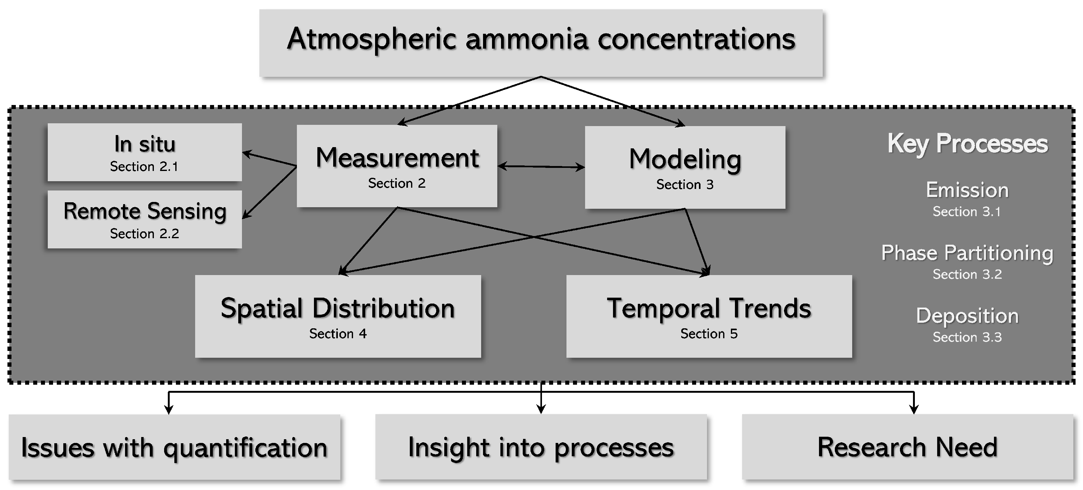
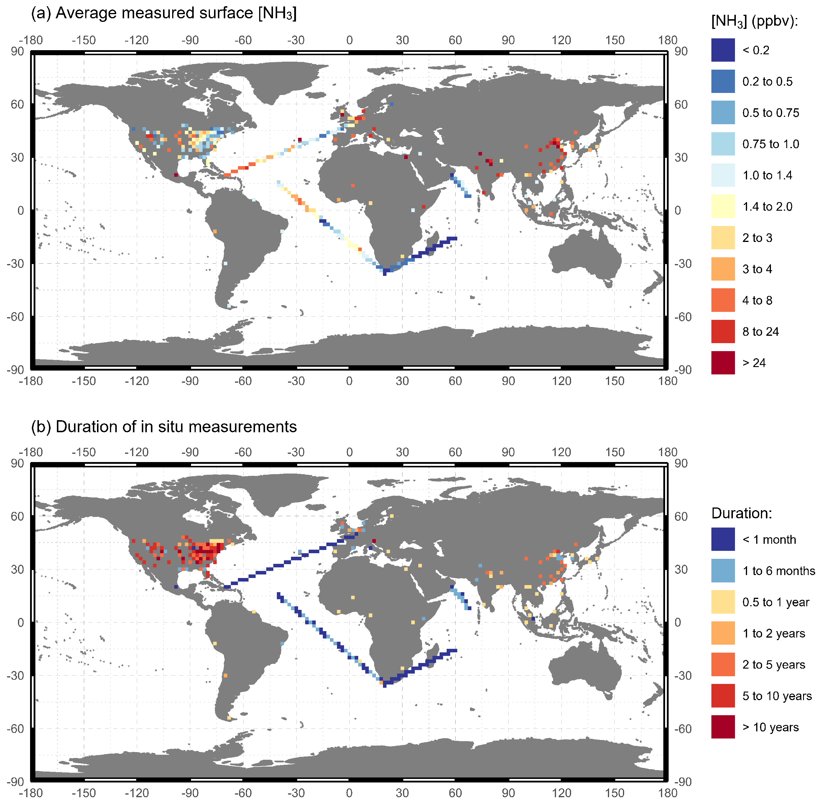
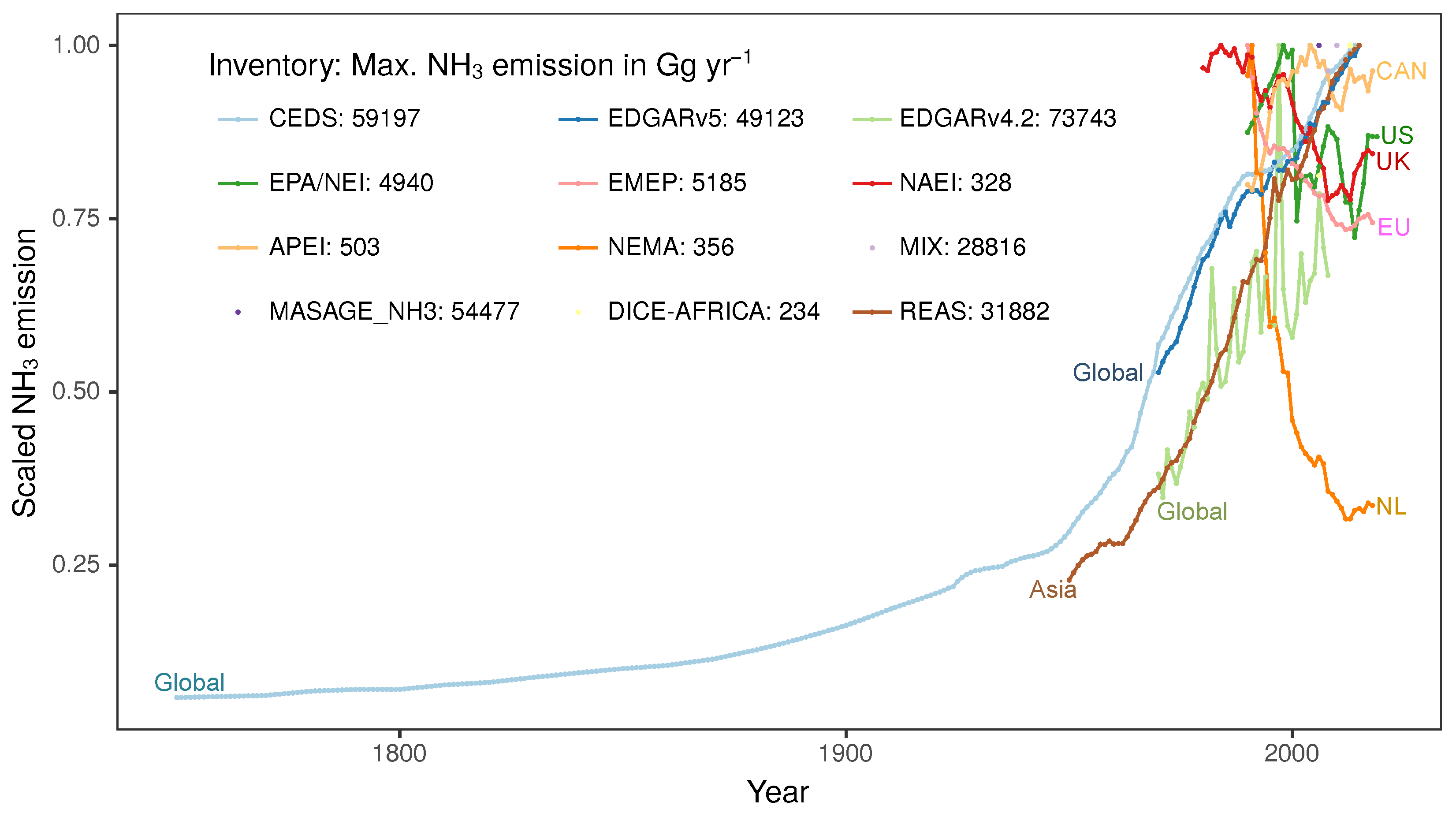
Table 1.
Details of long-term [NH3] measurement networks and their data access links.
| Network | Location | Start Year | Sites | Data Access |
|---|---|---|---|---|
| AMoN | US | 2007 | 123 | http://nadp.slh.wisc.edu/data/AMoN/ |
| AMoN-China | China | 2015 | 53 | https://doi.org/10.1021/acs.est.7b05235 |
| LML | Netherlands | 1993 | 8 | https://www.luchtmeetnet.nl/meetpunten?component=NH3 |
| MAN | Netherlands | 2005 | 300+ | https://man.rivm.nl/ |
| NAMN | UK | 1996 | 85 | https://uk-air.defra.gov.uk/networks/network-info?view=nh3 |
| NAPS | Canada | 2004 | 7 | http://maps-cartes.ec.gc.ca/rnspa-naps/data.aspx * |
* At the time of this review, this link did not contain the [NH3] data, which should be procurable from Yao and Zhang [61].
Table 2.
Some satellite remote sensing studies of atmospheric NH3 and instrumentation details.
| Reference | Region | Instrument | Period | Typical Concentration |
|---|---|---|---|---|
| [84] | Beijing | TES | 10 Jul 2007 | 5 to 25 ppbv |
| [86] | Global | IASI | 2008 | |
| [93] | Mediterranean basin | IASI | 25 Aug 2007 | 5.7 ± 0.1 × 10¹⁶ |
| [94] | Global | IASI | 2006 to 2009 (Various) | |
| [95] | California | IASI | 2008 | 3 to 10 ppbv |
| [87] | North Carolina | TES | 2002 | 1 to 6 ppbv |
| [96] | Global | IASI | Apr 2009 to Mar 2010 | |
| [97] | Central Russia | IASI | Jul and Sept 2010 | < 8 × 10¹⁷ |
| [92] | US | TES | Apr, Jul, and Oct 2006 to 2009 | |
| [98] | Global | IASI | 1 Nov 2007 to 31 Oct 2012 | < 1017 |
| [99] | California | TES | 16 Jan to 6 Feb 2013 | < 7 × 10¹⁶ |
| [100] | Global | TES | 2007 | |
| [101] | Canadian Oil Sands | TES | August to Sept 2013 | |
| [88] | Central US | CrIS | Jul 2005 | |
| [102] | Global | IASI | 2008 to 2013 | |
| [103] | FTIR Stations | IASI | 2008 to 2014 | |
| [104] | Global | MIPAS | 2003 to 2011 | |
| [89] | Global | AIRS | Sept 2002 to Aug 2015 | |
| [105] | Regional | AIRS | 2002 to 2016 | |
| [106] | California | TES | 7 May to 3 Jun 2010 | 21 ± 17 ppbv |
| [107] | North Africa | IASI | 7 May to 3 Jun 2010 | ≈ 1016 |
| [108] | Global | IASI | 2008 to 2017 | |
| [109] | Canada | IASI & CrIS | May 2016 | |
| [110] | Tanzania | IASI | 2008 to 2017 | < 4 × 10¹⁶ |
| [111] | Global | IASI | 2008 to 2017 | |
| [112] | Global | CrIS | 2013 to 2017 | 2 to 10 ppbv |
| [90] | Global | TANSO-FTS | 2009 to 2014 | ≈ 1016 |
| Instrument | Satellite | Agency | Period | Overpass | Field-of-View | Data Access |
|---|---|---|---|---|---|---|
| AIRS | Aqua | NASA | 2002–2016 | 13:30 | 13.5 km | https://dx.doi.org/10.5067/06YIT7GX74FN |
| CrIS | Suomi-NPP | NOAA | 2012–2017 | 13:30 | 14 km | https://hpfx.collab.science.gc.ca/~mas001/satellite_ext/cris/snpp/nh3/v1_5/ |
| IASI | MetOp-A/B/C | ESA | 2006–2020 | 09:30 | 12–39 km | https://iasi.aeris-data.fr/nh3/ |
| MIPAS | Envisat | ESA | 2002–2012 | N/A * | 420 km | http://share.lsdf.kit.edu/imk/asf/sat/mipas-export/ |
| TANSO-FTS | GOSAT | JAXA | 2009–2020 | 13:00 | 10.5 km | https://doi.org/10.5194/amt-13-309-2020 |
| TES | Aura | NASA | 2004-2018 | 13:30 | 5–8 km | https://dx.doi.org/10.5067/AURA/TES/TL2NH3N.008 |
Abbreviations: FTIR: Fourier-Transform InfraRed spectroscopy, AIRS: Atmospheric Infrared Sounder onboard NASA’s (National Aeronautics and Space Administration, US) Aqua satellite, CrIS: Cross-track Infrared Sounder onboard NOAA’s (National Oceanic and Atmospheric Administration, US) Suomi NPP satellite, IASI: Infrared Atmospheric Sounding Interferometer onboard the ESA’s (European Space Agency) MetOp satellites, MIPAS: Michelson Interferometer for Passive Atmospheric Sounding onboard ESA’s Envisat satellite, TANSO-FTS: Thermal And Near infrared Sensor for carbon Observations—Fourier Transform Spectrometer onboard JAXA’s (Japan Aerospace eXploration Agency) GOSAT-1, TES: Tropospheric Emission Spectrometer onboard NASA’s Aura satellite. Overpass refers to the daytime (when thermal contrast is optimal for NH3 retrieval) crossing of the equator. * Overpass not defined for MIPAS as it makes edge of the atmosphere (limb) NH3 retrievals.
Table 3.
Some modeling studies of atmospheric [NH3] using Eulerian chemical transport models.
| CTM | Equilibrium Model | Reference | Region | Period |
|---|---|---|---|---|
| CHIMERE | ISORROPIA | De Meij et al. [122] | Northern Italy | 2005 |
| CMAQ | MARS-A | Gilliland et al. [150] | Eastern US | 2001 |
| CMAQ | MARS-A | Gilliland et al. [126] | US | 2001 |
| DAMOS | Frohn [151] | Brandt et al. [120] | Europe, North America | |
| DAMOS | Frohn [151] | Geels et al. [121] | Denmark | 2007 |
| EMEP | EQSAM | Fagerli and Aas [116] | Europe | 1990–2003 |
| EMEP | EQSAM | Horvath et al. [117] | Hungary | 1990 and 1995–2004 |
| GEOS-Chem | ISORROPIA II | Heald et al. [91] | US | May 2009 to April 2010 |
| ISORROPIA II | Walker et al. [152] | California | 2009 | |
| RPMARES | Zhang et al. [153] | US | 2006 to 2008 | |
| ISORROPIA II | Schiferl et al. [34] | California | May and Jun 2010 | |
| ISORROPIA II | Paulot et al. [154] | Global oceanic | 1995–2004 | |
| RPMARES | Luo et al. [100] | Global | 2007 | |
| MARS-A | Zhu et al. [155] | Global and US | 2008 | |
| ISORROPIA II | Schiferl et al. [156] | US | 2008–2012 | |
| ISORROPIA II | Yu et al. [157] | US | 2001–2016 | |
| ISORROPIA II | Nair et al. [158] | US | 2001–2017 | |
| GEOS-Chem (adjoint) | ISORROPIA/MARS-A | Zhu et al. [92] | US | Apr, Jul, and Oct 2006–2009 |
| RPMARES | Paulot et al. [159] | US, E.U., China | 2005–2008 | |
| LOTOS-EUROS | Modified* CBM-IV | van Damme et al. [160] | Europe | 2008–2011 |
| MATCH | Langner et al. [123] | Baltic Sea Basin | 1996–2001 | |
| PMCAMx | ISORROPIA | Pinder et al. [130] | US | Jul and Oct 2001, Jan and Apr 2002 |
| Murphy and Pandis [127] | Eastern US | Jul 2001 | ||
| Tsimpidi et al. [128] | Mexico City | Apr 2003 | ||
| Karydis et al. [129] | Mexico City | Apr 2003 | ||
| Fountoukis et al. [131] | Europe | May 2008 | ||
| TM5 | EQSAM | de Meij et al. [115] | Europe | 2000 |
See Table S2 for details of Equilibrium Models. Abbreviations: CTM: Chemical Transport Model, CHIMERE:, CMAQ: Community Multiscale Air Quality, DAMOS: Danish Ammonia MOdeling System, EMEP: European Monitoring and Evaluation Programme, GEOS-Chem: Goddard Earth Observing System - Chemistry, LOTOS-EUROS: LOngTerm Ozone Simulation - EURopean Operational Smog, MATCH: Multi-scale Atmospheric Transport and Chemistry, PMCAMx:, TM5: Tracer Model 5. * Modification of the Carbon Bond Mechanism IV reaction mechanism with a scheme for NH4NO3 and (NH4)2SO4 by Zlatev [161].
Table 4.
Some modeling studies of atmospheric [NH3] using Lagrangian chemical transport models.
| CTM | Equilibrium Model | Reference | Region | Period |
|---|---|---|---|---|
| ACDEP | Modified* CBM-IV | Hertel et al. [135] | Denmark | 1990 |
| Hertel et al. [119] | Baltic Sea | 1999 | ||
| Gyldenkaerne et al. [136] | Northwestern Europe | 1999–2001 | ||
| de Leeuw et al. [137] | North Sea | 1999 | ||
| Skjøth et al. [138] | Denmark | 1998 and 1998 | ||
| Skjøth et al. [139] | Denmark | 1999 to 2001 | ||
| Skjøth et al. [140] | Europe | 2007 | ||
| AURAMS | Makar et al. [162] | Makar et al. [145] | North America | 2002 |
| FRAME | Barrett et al. [163] | Fournier et al. [164] | British Isles | 1996 |
| Fournier et al. [165] | British Isles | 1996 | ||
| Fournier et al. [166] | UK | 1996 | ||
| Dore et al. [167] | UK | 2002 | ||
| Sutton et al. [168] | UK | 2002–2004 | ||
| Tang et al. [169] | UK | 2012 | ||
| Vieno [170] | UK | 1999 | ||
| Sutton et al. [171] | UK | Sep 1996 to Nov 2000 | ||
| Sutton et al. [172] | UK | 1996 | ||
| Hellsten et al. [173] | UK | 2000 | ||
| Singles et al. [141] | Great Britain | 1987 to 1990 | ||
| Hallsworth et al. [174] | UK | 2002–2004 | ||
| Kryza et al. [142] | Poland | 2002–2005 | ||
| Zhang et al. [143] | North China Plain | 2008 | ||
| NAME | Meng and Seinfeld [175] | Redington and Derwent [144] | UK | 1996 |
| OPS | van Pul et al. [176] | Netherlands | Sep 2000 to 2001 | |
| van Jaarsveld [177] | Netherlands | Jan 1998 to Dec 2000 | ||
| van Pul et al. [146] | Eastern Netherlands | 2002–2003 | ||
| Stolk et al. [147] | Netherlands | 2005–2007 | ||
| van Pul et al. [146] | Netherlands | Jul 2002–Aug 2003 | ||
| Kruit et al. [148] | Netherlands | 1990–2014 | ||
| van der Swaluw et al. [178] | Netherlands | 1998–2002 | ||
| STILT-Chem | Wen et al. [149] | Wen et al. [149] | Canada | Jun to Nov 2006 |
| TERN | ApSimon et al. [132] | UK | 1983 | |
| TREND | Asman and van Jaarsveld [133] | Europe | 1990 | |
| Asman [134] | Denmark | 1996 |
Abbreviations: CTM: Chemical Transport Model, ACDEP: Atmospheric Chemistry and DEPosition, AURAMS: A Unified Regional Air quality Modeling System, FRAME: Fine Resolution AMmonia Exchange, NAME: Nuclear Accident ModEl, OPS: Operational Priority Substances, STILT-Chem: Stochastic Time-Inverted Lagrangian Transport and Chemistry, TERN: Transport over Europe of Reduced Nitrogen. * Modification of the Carbon Bond Mechanism IV reaction mechanism with a scheme for NH4NO3 and (NH4)2SO4 by Zlatev [161].
Table 5.
Global and regional ammonia emission inventories.
Abbreviations are noted in-text. * The original dataset at https://fpaulot.bitbucket.org/MASAGE/ was unavailable at the time of publication of this review article.
© 2020 by the authors. Licensee MDPI, Basel, Switzerland. This article is an open access article distributed under the terms and conditions of the Creative Commons Attribution (CC BY) license (http://creativecommons.org/licenses/by/4.0/).
Share and Cite
MDPI and ACS Style
Nair, A.A.; Yu, F. Quantification of Atmospheric Ammonia Concentrations: A Review of Its Measurement and Modeling. Atmosphere 2020, 11, 1092. https://doi.org/10.3390/atmos11101092
AMA Style
Nair AA, Yu F. Quantification of Atmospheric Ammonia Concentrations: A Review of Its Measurement and Modeling. Atmosphere. 2020; 11(10):1092. https://doi.org/10.3390/atmos11101092
Chicago/Turabian StyleNair, Arshad Arjunan, and Fangqun Yu. 2020. "Quantification of Atmospheric Ammonia Concentrations: A Review of Its Measurement and Modeling" Atmosphere 11, no. 10: 1092. https://doi.org/10.3390/atmos11101092
Note that from the first issue of 2016, this journal uses article numbers instead of page numbers. See further details here.