A Constructive Approach to Freyd Categories

Abstract

We discuss Peter Freyd’s universal way of equipping an additive category $\mathbf {P}$ with cokernels from a constructive point of view. The so-called Freyd category $\mathcal {A}(\mathbf {P})$ is abelian if and only if $\mathbf {P}$ has weak kernels. Moreover, $\mathcal {A}(\mathbf {P})$ has decidable equality for morphisms if and only if we have an algorithm for solving linear systems $X \cdot \alpha = \beta$ for morphisms $\alpha$ and $\beta$ in $\mathbf {P}$. We give an example of an additive category with weak kernels and decidable equality for morphisms in which the question whether such a linear system admits a solution is computationally undecidable. Furthermore, we discuss an additional computational structure for $\mathbf {P}$ that helps solving linear systems in $\mathbf {P}$ and even in the iterated Freyd category construction $\mathcal {A}( \mathcal {A}(\mathbf {P})^{\mathrm {op}} )$, which can be identified with the category of finitely presented covariant functors on $\mathcal {A}(\mathbf {P})$. The upshot of this paper is a constructive approach to finitely presented functors that subsumes and enhances the standard approach to finitely presented modules in computer algebra.

1 Introduction

With this paper, we hope to convince the reader that important parts of category theory such as the theory of Freyd categories are inherently algorithmic. To an additive category $\mathbf {P}$, Peter Freyd associated the so-called Freyd category $\mathcal {A}( \mathbf {P})$ [7, 13] that equips $\mathbf {P}$ with cokernels in a universal way. If we think of objects and morphisms in Freyd categories as data types, then theorems like the existence of kernels in $\mathcal {A}( \mathbf {P})$ (assuming $\mathbf {P}$ has weak kernels) can actually be proven by providing explicit constructions. Such constructions can in turn be directly implemented in computer algebra projects like Cap (Categories, Algorithms, Programming) [18, 19, 27] for performing effective computations. In this paper we provide various important constructions for Freyd categories.

Freyd categories have already played an important hidden role in computer algebra systems. A common data structure for finitely presented (left) modules over a ring R in computer algebra systems like Singular [12], Macaulay2 [16], or in a software project like homalg [20] written in GAP [14] is given by matrices over R, where an $(m \times n)$-matrix M is interpreted as the cokernel of its induced map between free row modules $R^{1 \times m} {\mathop {\longrightarrow }\limits ^{M}} R^{1 \times n}$. Performing operations like taking kernels in terms of this data structure can be seen as a special instance of performing those operations within a Freyd category, namely $\mathcal {A}( \mathrm {Rows}_R)$, the Freyd category associated to the additive category of row modules. We make this hidden role played by Freyd categories explicit and push it forward to reach new applications for computer algebra like the following computations with finitely presented functors, i.e., functors that are given as a cokernel of a natural transformation between representable functors:

• Determination of sets of natural transformations between two finitely presented functors like ${{\,\mathrm{\mathrm {Tor}}\,}}_1(M,-)$ and ${{\,\mathrm{\mathrm {Ext}}\,}}^i(A,-)$, where M and A are suitable R-modules (see Sect. 7.2).

• Construction of injective resolutions of finitely presented functors (Sect. 7.4).

• Deciding whether a given finitely presented functor is left exact (Sect. 7.3) or right exact (Sect. 7.5).

This paper is organized as follows. In Sect. 2 we briefly explain important aspects of Bishop’s constructive mathematics and why we chose it for the presentation of all algorithmic aspects of this paper. In Sect. 3 we give a constructive proof of the main theorem by Freyd [13] in a way such that a direct computer implementation becomes possible:

Given an additive category $\mathbf {P}$, then the category $\mathcal {A}( \mathbf {P})$ is abelian if and only if the category $\mathbf {P}$ has weak kernels.

To this end, we provide explicit constructions for sufficiently many operations in $\mathcal {A}( \mathbf {P})$ like taking (co)kernels and computing lifts/colifts along monomorphisms/epimorphisms. Moreover, decidability of equality for morphisms in $\mathcal {A}( \mathbf {P})$ is equivalent to the existence of an algorithm for solving linear systems $X \cdot \alpha = \beta$ for morphisms $\alpha$ and $\beta$ in $\mathbf {P}$.

In Sect. 4 we give several interpretations of Freyd categories. The Freyd category $\mathcal {A}( \mathrm {Rows}_R )$ provides a model for the category of finitely presented (left) modules over R (see Example 4.2) and a similar result holds for finitely presented graded modules (see Example 4.7). Moreover, we characterize so-called (left) computable rings, introduced by Barakat and Lange-Hegermann in [2], as those rings R for which $\mathcal {A}( \mathrm {Rows}_R )$ is abelian with decidable equality for morphisms.

Propositions that classically can be taken for granted have to be explicitly realized by algorithms in our constructive setup. In Sect. 5 and also in the end of Sect. 6 we provide examples of rings and categories with a curious behavior from a computational point of view:

• A ring with decidable equality, but the existence of a particular solution of left- and right-sided linear systems is computationally undecidable (Sect. 5.1).

• A ring P with decidable equality such that we can find particular solutions of left-sided linear systems, but the existence of a particular solution of right-sided linear systems is computationally undecidable (Sect. 5.2). It follows that $\mathcal {A}( \mathrm {Rows}_P )^{\mathrm {op}}$ has weak kernels and decidable equality for morphisms, but the problem whether a given linear system $X \cdot \alpha = \beta$ in $\mathcal {A}( \mathrm {Rows}_P )^{\mathrm {op}}$ admits a solution is computationally undecidable. Moreover, the iterated Freyd category $\mathcal {A}(\mathcal {A}( \mathrm {Rows}_P )^{\mathrm {op}})$ is abelian but its equality for morphisms is computationally undecidable (see Sect. 5.3).

• A commutative ring R that is not coherent (it has a finitely generated ideal that is not finitely presented), but we can find particular solutions of linear systems over R and the iterated Freyd category $\mathcal {A}(\mathcal {A}( \mathrm {Rows}_R )^{\mathrm {op}})$ is abelian with decidable linear systems in the sense of Definition 6.1 (see Theorem 6.18).

In Sect. 6 we study additive categories $\mathbf {P}$ equipped with homomorphism structures, where a homomorphism structure is a powerful tool that allows us to solve linear systems in $\mathbf {P}$. We describe our solving strategy in Theorem 6.10. This tool is also used in the determination of sets of natural transformations between finitely presented functors, with which we finally deal in the last Sect. 7.

The algorithms described in this paper are implemented in a GAP package [9] as a part of the Cap project [19]. Cap is a software project written in GAP and supports the programmer in the implementation of category theory based constructions. The algorithmic ideas in this paper were used in [8] in the context of sheaf cohomology computations over toric varieties.

Notation

We write morphisms between direct sums $A \oplus B \rightarrow C \oplus D$ in additive categories as matrices using the row convention $\begin{pmatrix} \gamma _{AC} &{} \gamma _{AD} \\ \gamma _{BC} &{} \gamma _{BD} \end{pmatrix}$ for morphisms $\gamma _{AC}: A \rightarrow C$, $\gamma _{AD}: A \rightarrow D$, $\gamma _{BC}: B \rightarrow C$, $\gamma _{BD}: B \rightarrow D$. We prefer writing $\alpha \cdot \beta : A \rightarrow C$ to $\beta \circ \alpha$ for the composition of morphisms $\alpha : A \rightarrow B$ and $\beta : B \rightarrow C$, since this matches the row convention in a way that composition of morphisms is simply given by matrix multiplication.

2 Constructive Category Theory

This paper aims at appealing both to practitioners of computer algebra and pure mathematicians with a background in abelian categories. In order to achieve this goal, the author had to decide on a language that

• on the one hand reveals the algorithmic nature of the presented constructions and gives a clear impression of how to implement them,

• on the other hand follows the aesthetics of pure mathematics by presenting theorems in an abstract and natural way.

The author felt that the usage of pseudocode certainly reveals the algorithmic nature of Freyd categories, but also distracts from the intrinsic beauty of the theory. In the end, the author chose the language of constructive mathematics as it is used by Erret Bishop and Fred Richman (see, e.g., [24]). The author did that for the following reasons: the language of Bishop’s constructive mathematics

• 1. reveals the algorithmic content of the theory of Freyd categories,

• 2. is perfectly suited for describing generic algorithms, i.e., constructions not depending on particular choices of data structures,

• 3. allows to express our algorithmic ideas without choosing some particular model of computation (like Turing machines),

• 4. all results stated in Bishop’s constructive mathematics are also valid classically,

• 5. does not differ very much from the classical language in our particular setup.

Before we elaborate on these points, here is a word of warning due to [25]: Bishop’s constructive mathematics cannot be directly interpreted within a topos in the sense that propositions about sets in Bishop’s constructive mathematics translate to propositions in the internal logic of an arbitrary topos. It is actually unclear how such a translation would look like, and even if there were such a translation, it could definitely not be valid in all toposes, since for example, the principle of countable choice is valid for Bishop. In particular, we do not claim in this paper that our results are valid or even interpretable in all toposes.

Now, we will elaborate more on Bishop’s constructive mathematics and how it serves our purpose stated in the beginning of this section. In Bishop’s constructive mathematics the notions of data types¹ and in particular of algorithms (or operations) are taken as primitives, i.e., notions that are not defined by other means. This idea is convincingly demonstrated in [24, Chapter I.1]:

Any attempt to define what an algorithm is ultimately involves an appeal to the notion of existence–for example, we might demand that there exist a step at which a certain computer program produces an output. If the term “exist” is used here in the classical sense, then we have failed to capture the constructive notion of an algorithm; if it is used in the constructive sense, then the definition is circular.

The notion of equality in Bishop’s constructive mathematics is conventional. This means that we need to explicitly define it as an equivalence relation on a given data type. In this way, a set can be defined as a data type together with a notion of equality. A function from a set A to a set B is an algorithm between the underlying data types of A and B that respects the notion of equality: equal input yields equal output.

Every proposition in Bishop’s constructive mathematics must have an algorithmic interpretation. As an example, we take a look at the property decidable equality, where we interpret the property that for all objects A, B in a category $\mathbf {A}$, we have

$$\begin{aligned} \forall \alpha , \beta \in {{\,\mathrm{\mathrm {Hom}}\,}}_{\mathbf {A}}(A,B): (\alpha = \beta ) \vee (\alpha \ne \beta ) \end{aligned}$$

as follows: we are given an algorithm that decides equality of a given pair of morphisms, i.e., that outputs a witness of $(\alpha = \beta )$ or $(\alpha \ne \beta )$. Note that a witness of equality can be understood as a term of the data type $(\alpha = \beta )$. For a concrete example of how such a witness between two morphisms being equal can look like, we refer to the equality witnesses in Definition 3.1. We will see throughout this paper that the idea of working explicitly with such witnesses comes in very handy for our purpose of an algorithmic description of Freyd categories.

Since propositions in Bishop’s constructive mathematics can be regarded as data types, and since data types do not carry an intrinsic notion of equality, the question of how to compare two terms of a proposition P, in particular for a proposition given by an equality type like $(\alpha = \beta )$, is again conventional. In this paper, we will not need to work with such “equalities between equalities”, even though the witnesses that we will meet may look “quite different from each other”. A theory that automatically provides a notion of equality for each type, and in particular for each equality type, is given by homotopy type theory [30]. Note that the fact that we do not need to define equality between terms of a data type in Bishop’s constructive mathematics is particularly handy in category theory, where building too much upon the notion of equality between objects of a category usually leads to breaking the principle of equivalence [26]. Thus, for us, the objects in a category will simply be a data type. Note that in homotopy type theory, equality of objects is beautifully dealt with by identifying the equality type of objects with the type encoding “being isomorphic” [30, Chapter on category theory].

To give another example for the interpretation of a proposition in Bishop’s constructive mathematics, we interpret for a given additive category $\mathbf {A}$ the following property:

$\mathbf {A}$ has kernels.

We deliberately provide a very verbose interpretation for the sake of clarity:

• We have an algorithm with the following specification:

  • It takes as input $A,B \in \mathrm {Obj}_{\mathbf {A}}$, $\alpha \in {{\,\mathrm{\mathrm {Hom}}\,}}_{\mathbf {A}}(A,B)$.

  • It outputs an object ${{\,\mathrm{\mathrm {ker}}\,}}( \alpha ) \in \mathrm {Obj}_{\mathbf {A}}$, a morphism

    $$\begin{aligned}\mathrm {KernelEmbedding}( \alpha ) \in {{\,\mathrm{\mathrm {Hom}}\,}}_{\mathbf {A}}({{\,\mathrm{\mathrm {ker}}\,}}( \alpha ), A),\end{aligned}$$

    and a witness of

    $$\begin{aligned} \mathrm {KernelEmbedding}( \alpha ) \cdot \alpha = 0.\end{aligned}$$

• Furthermore, we have an algorithm with the following specification:

  • It takes as input $A,B,T \in \mathrm {Obj}_{\mathbf {A}}$, $\alpha \in {{\,\mathrm{\mathrm {Hom}}\,}}_{\mathbf {C}}(A,B)$, $\tau \in {{\,\mathrm{\mathrm {Hom}}\,}}_{\mathbf {A}}(T,A)$, and a witness of $\tau \cdot \alpha = 0$.

  • It outputs a morphism $u \in {{\,\mathrm{\mathrm {Hom}}\,}}_{\mathbf {A}}(T,{{\,\mathrm{\mathrm {ker}}\,}}( \alpha ))$, a witness of

    $$\begin{aligned} u \cdot \mathrm {KernelEmbedding}( \alpha ) = \tau ,\end{aligned}$$

    and a witness of u being uniquely determined up to $=$ by this property. Note that a witness of u being uniquely determined in this context consists of an algorithm with the following specification:

    • It takes as input a morphism $v \in {{\,\mathrm{\mathrm {Hom}}\,}}_{\mathbf {A}}(T,{{\,\mathrm{\mathrm {ker}}\,}}( \alpha ))$ and a witness for $v \cdot \mathrm {KernelEmbedding}( \alpha ) = \tau$.

    • It outputs a witness of $u = v$.

Stating a property in Bishop’s constructive mathematics usually is not done in such a verbose way, but uses common expressions like “P holds” for a property P instead of “we have a witness of P”. We will also use such abbreviations, in order to facilitate a classical reading. In the Appendix A we listed a constructive interpretation of various kinds of categories, e.g., additive or abelian categories (cf. the corresponding list in [3, Appendix B] and note the difference in our treatment of equalities for morphisms explained in Remark A.2).

Remark 2.1

(Bishop’s constructive mathematics for practitioners of computer algebra) There are at least two major concerns which a practitioner of computer algebra might have when looking at Bishop’s constructive mathematics: the verbosity w.r.t. witnesses of the input/output of algorithms and the question of their efficiency.

Indeed, in standard computer algebra systems like GAP [14], properties of mathematical objects are usually regarded as a mere boolean value: $\mathtt {true}$ or $\mathtt {false}$. For example, an algorithm that expects a monomorphism as an input in such a system is given by an operation that takes as input a homomorphism for which the property of being mono is set to $\mathtt {true}$, it does not expect a witness for being mono as an additional argument. In practice, this is a good choice since it does not burden the user who wants to perform some quick computations to provide such a verbose input.

We argue that the language of Bishop’s constructive mathematics nevertheless is useful for computer algebra, and that the verbosity of the input/output can be understood as a theoretical asset rather than an obstacle:

• 1. An algorithm implemented in a standard computer algebra system which relies on the fact that the input is a monomorphism but which simply gets a homomorphism as an input often implicitly builds a witness of being monomorphism during the computation. For example, in Construction 3.14, we rely on having a witness of being a monomorphism², and in a standard computer algebra system, this algorithm would be implemented by first calling an oracle that actually provides such a witness. Thus, using the language of Bishop’s constructive mathematics, programmers who use standard computer algebra systems may benefit by getting a very clear idea about what oracles have to exist in order to make their implementations work.

• 2. The fact that the output of an algorithm in Bishop’s constructive mathematics needs to be verbose actually complies with the paradigm that no already computed knowledge should be lost. Often, algorithms in standard computer algebra systems produce witnesses within a computation, but cut the output to a simple $\mathtt {true}$ or $\mathtt {false}$. If we retain those witnesses and pass them to other algorithms which need them as input, we may save costly calls of oracles. An example of a computer algebra problem³ where this philosophy was successfully applied can be found in [28].

• 3. The verbosity can also be seen as a way to analyze under which conditions an algorithm can theoretically be performed, even in contexts where witnesses are usually not available.

The issue of efficiency of algorithms in Bishop’s constructive mathematics can be approached pragmatically: the algorithms suggested in Sect. 3 translate in the case of finitely presented modules over a computable ring R to implementations that are actually used in computer algebra, e.g., within homalg [20]. Thus, Bishop’s constructive mathematics does not lead to slow algorithms per se, it is rather the case that the practitioner of computer algebra who needs a fast algorithm will certainly not be satisfied with just any algorithm that does the job. The computer algebraist will keep looking for “the most efficient” method. And as we argued before, the verbosity of Bishop’s constructive mathematics can actually be an asset in the pursuit of that goal.

In his review of Mines, Richman, and Ruitenburg’s book on constructive algebra [24] Beeson argues for more interaction between computer algebra and constructive mathematics [6]:

The followers of Bishop ought to read the literature in symbolic computations. The algorithmic algebraists could benefit considerably from reading both Bishop and the volume under review.

The author believes that such an interaction can indeed be very fruitful, and hopes that this paper serves as an example of such an interaction.

Remark 2.2

(Bishop’s constructive mathematics for classical mathematicians) This paper may very well be read classically⁴. The sets of Bishop’s constructive mathematics may be interpreted as classical sets in which the notion of equality is given by the provided equivalence relation (i.e., the quotient set of the more setoid-like Bishop set). In this way, the notion of a function can also be translated by a classical function (see [25]). We hope that in this way, we achieve our goal that our paper also appeals to pure mathematicians with a background in abelian categories.

Remark 2.3

One goal of this paper is to describe Freyd categories within Bishop’s constructive mathematics (Sect. 3). However, it is not our goal to do the same for categories that classically turn out to be equivalent to Freyd categories, like the category of finitely presented functors. Thus, we allow ourselves to work classically whenever we interpret Freyd categories in terms of other categories (this happens in Sect. 4 and in Sect. 7). The reason for this is pragmatic: we want to demonstrate the usefulness of having Freyd categories computationally available, and we believe that this can be done by interpreting Freyd categories in terms of other categories that classical mathematicians care about.

3 Constructive Freyd Categories

There are several ways to think about Freyd categories. In Definition 3.1, we will introduce Freyd categories within Bishop’s constructive mathematics and give names to usually nameless entities, like witnesses. Peter Freyd’s original definition [13, Preproof of Theorem 1.4] is exactly ours if we apply a classical reading (see Remark 2.2).

Let $\mathbf {P}$ be an additive category. Morally, Freyd categories provide a universal way to add cokernels to $\mathbf {P}$. This can for example⁵ be made precise by saying that the inclusion of additive categories with cokernels and cokernel preserving functors into the (big) category of all additive categories has a left adjoint, given by the Freyd category construction.

A quick way to state their definition is possible if $\mathbf {P}$ is idempotent complete. Then, the Freyd category of $\mathbf {P}$ is the quotient of the category of arrows of $\mathbf {P}$ by all split epimorphisms [7, Definition 3.1]. Since we do not assume $\mathbf {P}$ to be idempotent complete, we prefer to work with Freyd’s original definition.

Definition 3.1

Let $\mathbf {P}$ be an additive category. The Freyd category $\mathcal {A}(\mathbf {P})$ is given by the following data:

• 1. An object in $\mathcal {A}(\mathbf {P})$ is simply a morphism in $\mathbf {P}$. We will write $(A {\mathop {\longleftarrow }\limits ^{\rho _A}} R_A)$ for such an object, even though $R_A$ and $\rho _A$ do not formally depend⁶ on A.

• 2. A morphism in $\mathcal {A}(\mathbf {P})$ from $(A {\mathop {\longleftarrow }\limits ^{\rho _A}} R_A)$ to $(B {\mathop {\longleftarrow }\limits ^{\rho _B}} R_B)$ is given by a morphism $A {\mathop {\longrightarrow }\limits ^{\alpha }} B$ in $\mathbf {P}$ such that there exists another morphism $R_A {\mathop {\longrightarrow }\limits ^{\rho _{\alpha }}} R_B$ rendering the diagram

  

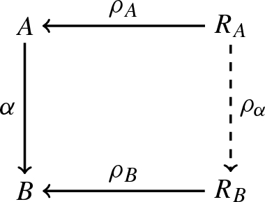
  commutative. We call $\alpha$ the morphism datum and any such $\rho _{\alpha }$ a morphism witness. We often write $\{\alpha , \rho _{\alpha }\}$ for a morphism in $\mathcal {A}(\mathbf {P})$ to highlight a particular choice of a morphism witness $\rho _{\alpha }$ for a morphism datum $\alpha$. We define two morphisms $A {\mathop {\longrightarrow }\limits ^{\alpha }} B$, $A {\mathop {\longrightarrow }\limits ^{\alpha '}} B$ from $(A {\mathop {\longleftarrow }\limits ^{\rho _A}} R_A)$ to $(B {\mathop {\longleftarrow }\limits ^{\rho _B}} R_B)$ to be equal (in $\mathcal {A}(\mathbf {P})$) if there exists a lift $\lambda$ as in the following diagram:

  

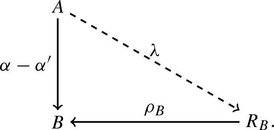
  We call any such morphism $\lambda$ a witness for $\alpha$ and $\alpha '$ being equal.

• 3. Composition and identities are directly inherited from $\mathbf {P}$.

Remark 3.2

Being equal in $\mathcal {A}( \mathbf {P})$ clearly defines an equivalence relation (transitivity corresponds to addition of witnesses) that is compatible with composition. Furthermore, $\mathcal {A}( \mathbf {P})$ inherits the structure of an additive category from the category of arrows of $\mathbf {P}$.

Remark 3.3

Since we are interested in a constructive approach to Freyd categories, we say a few words about witnesses. Classically, morphisms in the Freyd category are the equivalence classes of “being equal in $\mathcal {A}( \mathbf {P})$”. For us, however, it is more convenient to use the language of morphism data and witnesses since these are the actual entities for which we define our algorithms (see Constructions 3.6, 3.11, 3.14, 3.15). In particular, we avoid unnecessary picking of representatives in the beginning of all these constructions.

Stating the main theorem for $\mathcal {A}(\mathbf {P})$ requires another definition.

Definition 3.4

Let $\mathbf {P}$ be an additive category. For a morphism $\alpha : A \rightarrow B$ in $\mathbf {P}$, a weak kernel consists the following data:

• (1) An object $K \in \mathbf {P}$.

• (2) A morphism $\kappa : K \rightarrow A$ such that $\kappa \cdot \alpha = 0$.

• (3) An operation that constructs for $T \in \mathbf {P}$ and any test morphism $\tau : T \rightarrow A$ such that $\tau \cdot \alpha = 0$ a morphism $u(\tau ): T \rightarrow K$ with $u(\tau ) \cdot \kappa = \tau$.

  

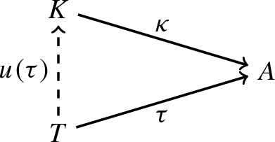
Note that the morphism $u(\tau )$ does not have to be unique with this property, so we really weaken the usual definition of a kernel. Furthermore, we say $\mathbf {P}$ has weak kernels if it comes equipped with an operation constructing the triple $(K,\kappa ,u)$ for given $\alpha$.

The following main theorem about $\mathcal {A}( \mathbf {P})$ is due to Freyd [13].

Theorem 3.5

Let $\mathbf {P}$ be an additive category. Then $\mathcal {A}(\mathbf {P})$ is an abelian category if and only if $\mathbf {P}$ has weak kernels.

Freyd gives two proofs of his theorem: a non-elementary one using functor categories [13, Proposition 1.4] and a more elementary one using an auxiliary theorem for recognizing abelian categories via the existence of factorizations of morphisms into cokernel projections and kernel embeddings [13, Section 3]. Our goal is to render Theorem 3.5 constructive in a way such that a direct computer implementation becomes possible. To this end, we will state and prove the explicit construction steps for (co)kernels (and their universal properties) in $\mathcal {A}(\mathbf {P})$, as well as for lifts along monomorphisms and colifts along epimorphisms. Our explicitness reveals what is otherwise hidden in propositions, namely the important role of witnesses for the construction of morphism data.

3.1 Cokernels in Freyd Categories

We start with the construction of cokernels.

Construction 3.6

(Cokernels) Given a morphism

$$\begin{aligned} \{\alpha , \rho _{\alpha }\}: (A {\mathop {\longleftarrow }\limits ^{\rho _A}} R_A) \longrightarrow (B {\mathop {\longleftarrow }\limits ^{\rho _B}} R_B) \end{aligned}$$

in $\mathcal {A}(\mathbf {P})$, the following diagram shows us how to construct its cokernel projection along with the universal property:

How to read this diagram: the solid arrow pointing up right is the cokernel projection, the solid arrow pointing down right is a test morphism for the universal property of the cokernel, and the dashed arrow pointing straight down is the morphism induced by the universal property. The dotted arrow labeled with $\sigma$ is a witness for the composition $\{\alpha , \rho _\alpha \} \cdot \{\tau ,\rho _{\tau }\}$ being zero, i.e., it denotes a morphism $\sigma : A \rightarrow R_T$ such that $\sigma \cdot \rho _T = \alpha \cdot \tau$. We see that $\sigma$ is used in the construction of the morphism witness for the induced morphism, but not in any morphism data. We also see that no morphism witness is used for the construction of any morphism data.

Correctness of the construction

It is an easy calculation that all morphisms are well-defined. A witness for the composition $\{\alpha , \rho _\alpha \} \cdot \{\mathrm {id}_B, \begin{pmatrix}\mathrm {id}_{R_B}&0\end{pmatrix}\}$ being zero is given by the natural inclusion $A \hookrightarrow R_B \oplus A$. The commutativity of the triangle even holds strictly in the category of arrows of $\mathbf {P}$. For the uniqueness of the induced morphism, it suffices to see that our construction of the cokernel projection is an epimorphism, which follows from the next Lemma 3.7. $\square$

Lemma 3.7

Every morphism in $\mathcal {A}(\mathbf {P})$ of the form

$$\begin{aligned} \{\mathrm {id}_A, \rho \}: (A {\mathop {\longleftarrow }\limits ^{\rho _1}} R_1) \longrightarrow (A {\mathop {\longleftarrow }\limits ^{\rho _2}} R_2) \end{aligned}$$

is an epimorphism.

Proof

See also [13, first part of the proof of Lemma 3.2.1]. Given a test morphism for $\{\mathrm {id}_A, \rho \}$ being an epimorphism, i.e., a morphism

$$\begin{aligned} \{\beta , \rho _{\beta }\}: (A {\mathop {\longleftarrow }\limits ^{\rho _2}} R_2) \longrightarrow (B {\mathop {\longleftarrow }\limits ^{\rho _B}} R_B) \end{aligned}$$

such that $\{\mathrm {id}_A, \rho \} \cdot \{\beta , \rho _{\beta }\} = 0$, we can take any witness $\sigma : A \rightarrow R_B$ for this composition being zero as a witness for $\{\beta , \rho _{\beta }\}$ being zero. $\square$

Remark 3.8

Given two morphisms $\{\alpha , \rho _\alpha \}$ and $\{\beta , \rho _\beta \}$ which are equal in $\mathcal {A}(\mathbf {P})$ but for which $\alpha \ne \beta$ in $\mathbf {P}$, the constructed cokernel objects of Construction 3.6 may look quite different from each other. This is no problem since, as we explained in Sect. 2, equality is a conventional notion in Bishop’s constructive mathematics, and we do not impose a notion of equality on the data type of objects.

3.2 Kernels in Freyd Categories

For the construction of kernels in $\mathcal {A}(\mathbf {P})$, we first introduce weak pullbacks in $\mathbf {P}$ (mainly for introducing our notation).

Definition 3.9

Let $\mathbf {P}$ be an additive category. For a given cospan $A {\mathop {\longrightarrow }\limits ^{\alpha }} B {\mathop {\longleftarrow }\limits ^{\gamma }} C$ in $\mathbf {P}$, a weak pullback consists the following data:

• 1. An object $A \times _B C \in \mathbf {P}$.

• 2. Morphisms $\begin{bmatrix}1\\ 0\end{bmatrix} : A \times _B C \rightarrow A$ and $\begin{bmatrix}0\\ 1\end{bmatrix} : A \times _B C \rightarrow C$ such that $\begin{bmatrix}1\\ 0\end{bmatrix} \cdot \alpha = \begin{bmatrix}0\\ 1\end{bmatrix} \cdot \gamma$.

• 3. An operation that constructs for $T \in \mathbf {P}$ and morphisms $p: T \rightarrow A$, $q: T \rightarrow C$ such that $p \cdot \alpha = q \cdot \gamma$ a morphism $\begin{bmatrix}{p}&{q} \end{bmatrix} : T \rightarrow A \times _B C$ satisfying

  $$\begin{aligned} \begin{array}{ccccc} p = \begin{bmatrix}{p} &{} {q} \end{bmatrix} \cdot \begin{bmatrix}1\\ 0\end{bmatrix}&\,&\text { and }&\,&q = \begin{bmatrix}{p} &{} {q} \end{bmatrix} \cdot \begin{bmatrix}0\\ 1\end{bmatrix} . \end{array} \end{aligned}$$

Note that the morphism $\begin{bmatrix}{p}&{q} \end{bmatrix}$ does not have to be unique with this property, so we really weaken the usual definition of a pullback. Also note that we use square matrices for weak pullback morphisms (in contrast to round matrices for direct sum morphisms).

Remark 3.10

If $\mathbf {P}$ has weak kernels, then it also has weak pullbacks, since we can compute weak pullbacks from weak kernels and direct sums in the same way as we can compute pullbacks from kernels and direct sums.

Construction 3.11

(Kernels) Given a morphism

$$\begin{aligned} \{\alpha , \rho _{\alpha }\}: (A {\mathop {\longleftarrow }\limits ^{\rho _A}} R_A) \longrightarrow (B {\mathop {\longleftarrow }\limits ^{\rho _B}} R_B) \end{aligned}$$

in $\mathcal {A}(\mathbf {P})$, the following diagram shows us how to construct its kernel embedding along with the universal property:

How to read this diagram: the occurring weak pullbacks are defined by

The solid arrow pointing down right is the kernel embedding, the solid arrow pointing up right is a test morphism for the universal property of the kernel, and the dashed arrow pointing straight up is the morphism induced by the universal property. The dotted arrow depicts $\sigma : T \rightarrow R_B$, a witness for the composition $\{\tau ,\rho _{\tau }\} \cdot \{\alpha , \rho _\alpha \}$ being zero. We see that no morphism witness is used for the construction of any morphism data. But now, in contrast to the cokernel construction, the witness $\sigma$ is used in the construction of the morphism datum of the induced morphism.

Correctness of the construction

It is easy to see that all morphisms are well-defined. A witness for the composition $\left\{ \begin{bmatrix}0\\ 1\end{bmatrix} , \begin{bmatrix}0\\ 1\end{bmatrix} \right\} \cdot \{\alpha , \rho _\alpha \}$ being zero is given by the projection $\begin{bmatrix}1\\ 0\end{bmatrix} : R_B\times _B A \rightarrow R_B$. The commutativity of the triangle even holds strictly in the category of arrows of $\mathbf {P}$. For the uniqueness of the induced morphism, it suffices to see that our construction of the kernel embedding is a monomorphism, which follows from the next Lemma 3.12. $\square$

Lemma 3.12

Given a cospan $A {\mathop {\longrightarrow }\limits ^{\alpha }} B {\mathop {\longleftarrow }\limits ^{\gamma }} C$ in $\mathbf {P}$, the morphism in $\mathcal {A}(\mathbf {P})$ defined by

$$\begin{aligned} \left\{ \alpha , \begin{bmatrix}0\\ 1\end{bmatrix} \right\} : (A {\mathop {\longleftarrow }\limits ^{ \begin{bmatrix}1\\ 0\end{bmatrix} }} A\times _B C) \longrightarrow (B {\mathop {\longleftarrow }\limits ^{\gamma }} C) \end{aligned}$$

is a monomorphism.

Proof

See also [13, first part of proof of Lemma 3.2.2]. Given a test morphism for $\left\{ \alpha , \begin{bmatrix}0\\ 1\end{bmatrix} \right\}$ being a monomorphism, i.e., a morphism

$$\begin{aligned} \{\delta , \rho _{\delta }\}: (D {\mathop {\longleftarrow }\limits ^{\rho _D}} R_D) \longrightarrow (A {\mathop {\longleftarrow }\limits ^{ \begin{bmatrix}1\\ 0\end{bmatrix} }} A\times _B C) \end{aligned}$$

such that $\{\delta , \rho _{\delta }\} \cdot \left\{ \alpha , \begin{bmatrix}0\\ 1\end{bmatrix} \right\} = 0$, take a witness $\sigma : D \rightarrow C$ for this composition being zero. Then $\begin{bmatrix}{\delta }&{\sigma } \end{bmatrix} : D \rightarrow A \times _B C$ is a witness for $\{\delta , \rho _{\delta }\}$ being zero. $\square$

3.3 Lift Along Monomorphisms in Freyd Categories

One axiom of abelian categories states that every monomorphism is the kernel of its cokernel. When we rephrase this axiom constructively, we see that we have to be able to construct lifts along monomorphisms (see Definition A.8).

Remark 3.13

We remind the reader that the witnesses which occur in the beginning of the following construction are actually part of the input of the described algorithm. This is due to the untruncated propositions as type logic underlying Bishop’s constructive mathematics, see Sect. 2.

Construction 3.14

(Lifts along monomorphisms) The kernel embedding of a given monomorphism

$$\begin{aligned} \{\alpha , \rho _{\alpha }\}: (A {\mathop {\longleftarrow }\limits ^{\rho _A}} R_A) \longrightarrow (B {\mathop {\longleftarrow }\limits ^{\rho _B}} R_B) \end{aligned}$$

in $\mathcal {A}(\mathbf {P})$ is zero. A witness of this fact is given by a morphism $\sigma : R_B \times _B A \rightarrow R_A$ such that

$$\begin{aligned} \begin{bmatrix}0\\ 1\end{bmatrix} = \sigma \cdot \rho _A \end{aligned}$$

(3.1)

(see Construction 3.11). Now, the following diagram shows us how to construct a lift along $\{\alpha , \rho _{\alpha }\}$ for a given test morphism:

How to read this diagram: the solid horizontal arrow is the cokernel projection of our monomorphism $\{\alpha , \rho _{\alpha }\}$ (see Construction 3.6). The dotted arrow is a witness for the composition of the test morphism $\{\tau , \rho _{\tau }\}$ with the cokernel projection being zero. The upwards pointing dashed arrow is the desired lift, whose morphism witness involves the weak pullback induced morphism given by the diagram

Correctness of the construction

$\begin{pmatrix}{\tau _{R_B}}&{\tau _A} \end{pmatrix}$ being a witness gives the equation

$$\begin{aligned} \tau _{R_B} \cdot \rho _B + \tau _A \cdot \alpha = \tau \end{aligned}$$

(3.2)

from which we can already see that if the constructed lift is well-defined as a morphism in $\mathcal {A}(\mathbf {P})$, then it really is a lift along our monomorphism. So we have to check that the morphism witness of our lift is correct. Multiplying (3.2) with $\rho _T$ from the left yields

$$\begin{aligned} \rho _T \cdot \tau _{R_B} \cdot \rho _B + \rho _T \cdot \tau _A \cdot \alpha = \rho _T \cdot \tau = \rho _{\tau } \cdot \rho _B \end{aligned}$$

(3.3)

and thus

$$\begin{aligned} (\rho _{\tau } - \rho _T \cdot \tau _{R_B}) \cdot \rho _B = (\rho _T \cdot \tau _A) \cdot \alpha \end{aligned}$$

(3.4)

which proves that the weak pullback induced morphism $\begin{bmatrix}{\rho _{\tau }-\rho _T \cdot \tau _{R_B}}&{\rho _T \cdot \tau _A} \end{bmatrix}$ is well-defined. Last, we compute

$$\begin{aligned} \rho _T \cdot \tau _A =&\begin{bmatrix}{\rho _{\tau }-\rho _T \cdot \tau _{R_B}}&{\rho _T \cdot \tau _A} \end{bmatrix} \cdot \begin{bmatrix}0\\ 1\end{bmatrix} \\&{\mathop {=}\limits ^{(3.1)}} \begin{bmatrix}{\rho _{\tau }-\rho _T \cdot \tau _{R_B}}&{\rho _T \cdot \tau _A} \end{bmatrix} \cdot \sigma \cdot \rho _A \end{aligned}$$

which shows that the morphism witness is correct. $\square$

3.4 Colifts Along Epimorphisms in Freyd Categories

Dually, we have to be able to construct colifts along epimorphisms in $\mathcal {A}(\mathbf {P})$ (see Definition A.8).

Construction 3.15

(Colifts along epimorphisms) The cokernel projection of a given epimorphism

$$\begin{aligned} \{\alpha , \rho _{\alpha }\}: (A {\mathop {\longleftarrow }\limits ^{\rho _A}} R_A) \longrightarrow (B {\mathop {\longleftarrow }\limits ^{\rho _B}} R_B) \end{aligned}$$

in $\mathcal {A}(\mathbf {P})$ is zero. A witness of this fact is given by a morphism $\begin{pmatrix}{\sigma _{R_B}}&{\sigma _A} \end{pmatrix} : B \rightarrow R_B \oplus A$ such that

$$\begin{aligned} \sigma _{R_B} \cdot \rho _B + \sigma _A \cdot \alpha = \mathrm {id}_B \end{aligned}$$

(3.5)

(see Construction 3.6). Now, the following diagram shows us how to construct a colift along $\{\alpha , \rho _{\alpha }\}$ for a given test morphism:

How to read this diagram: the solid horizontal arrow is the kernel embedding of our epimorphism $\{\alpha , \rho _{\alpha }\}$ (see Construction 3.11), where we set $R_K :=(R_B \times _B A) \times _A R_A$. The dotted arrow is a witness for the composition of the kernel embedding with the test morphism $\{\tau , \rho _{\tau }\}$ being zero. The downwards pointing dashed arrow is the desired colift, whose morphism witness involves the weak pullback induced morphism given by the diagram

Correctness of the construction

Multiplying (3.5) with $\rho _B$ from the left yields

$$\begin{aligned} \rho _B \cdot \sigma _{R_B} \cdot \rho _B + \rho _B \cdot \sigma _A \cdot \alpha = \rho _B \end{aligned}$$

(3.6)

and thus

$$\begin{aligned} (\rho _B \cdot \sigma _A) \cdot \alpha = ( \mathrm {id}_{R_B} - \rho _B \cdot \sigma _{R_B} ) \cdot \rho _B \end{aligned}$$

(3.7)

which shows that $\begin{bmatrix}{\mathrm {id}_{R_B} - \rho _B\cdot \sigma _{R_B}}&{\rho _B \cdot \sigma _A} \end{bmatrix}$ is well-defined. Well-definedness of the constructed colift as a morphism in $\mathcal {A}(\mathbf {P})$ follows from the commutativity of the two inner squares in the diagram

It remains to show that the constructed colift really yields a colift for the given test morphism. To this end, we multiply (3.5) with $\alpha$ from the left

$$\begin{aligned} \alpha \cdot \sigma _{R_B} \cdot \rho _B + \alpha \cdot \sigma _A \cdot \alpha = \alpha \end{aligned}$$

(3.8)

and obtain

$$\begin{aligned} (\alpha \cdot \sigma _{R_B}) \cdot \rho _B = ( \mathrm {id}_A - \alpha \cdot \sigma _A) \cdot \alpha \end{aligned}$$

(3.9)

which shows that $\begin{bmatrix}{\alpha \cdot \sigma _{R_B}}&{\mathrm {id}_A - \alpha \cdot \sigma _A} \end{bmatrix} : A \rightarrow R_B \times _B A$ is well-defined. Last, we compute

$$\begin{aligned} \begin{bmatrix}{\alpha \cdot \sigma _{R_B}}&{\mathrm {id}_A - \alpha \cdot \sigma _A} \end{bmatrix} \cdot \sigma \cdot \rho _{T}&= \begin{bmatrix}{\alpha \cdot \sigma _{R_B}}&{\mathrm {id}_A - \alpha \cdot \sigma _A} \end{bmatrix} \cdot \begin{bmatrix}0\\ 1\end{bmatrix} \cdot \tau \\&=(\mathrm {id}_A - \alpha \cdot \sigma _A)\cdot \tau \\&={\tau - \alpha \cdot \sigma _A}\cdot \tau \\ \end{aligned}$$

and see that we have found a witness for $\tau$ and $\alpha \cdot (\sigma _A\cdot \tau )$ being equal in $\mathcal {A}(\mathbf {P})$. $\square$

3.5 A Constructive Proof of the Main Theorem

Proof of Theorem 3.5

Construction 3.6 shows that $\mathcal {A}( \mathbf {P})$ always has cokernels. Moreover, if $\mathbf {P}$ has weak kernels, then Constructions 3.11, 3.14, 3.15 show that $\mathcal {A}(\mathbf {P})$ is abelian. For the other direction, we construct weak kernels in $\mathbf {P}$ using the operation for kernels in $\mathcal {A}(\mathbf {P})$: given a morphism $A {\mathop {\longrightarrow }\limits ^{\alpha }} B \in \mathbf {P}$, we compute a kernel embedding

$$\begin{aligned}\{\kappa , \rho _{\kappa }\}: (K {\mathop {\longleftarrow }\limits ^{\rho _K}} R_K) \longrightarrow (A \longleftarrow 0)\end{aligned}$$

of $\{\alpha ,0\}:(A \longleftarrow 0) \longrightarrow (B \longleftarrow 0)$. Then $\kappa \cdot \alpha = 0 \in \mathbf {P}$ since any witness for $\{\kappa , \rho _{\kappa }\}\cdot \{\alpha ,0\}$ being zero in $\mathcal {A}(\mathbf {P})$ factors over 0. Thus, $\kappa : K \rightarrow A$ is a candidate for a weak kernel embedding of $\alpha$ in $\mathbf {P}$. Let $T {\mathop {\longrightarrow }\limits ^{\tau }} A \in \mathbf {P}$ such that $\tau \cdot \alpha = 0 \in \mathbf {P}$. We use the universal property of the kernel in $\mathcal {A}(\mathbf {P})$ to compute the dashed arrow in the following commutative diagram:

Again, from $\{u, \rho _u\} \cdot \{\kappa , \rho _{\kappa }\} = \{\tau ,0\} \in \mathcal {A}(\mathbf {P})$ we can deduce $u \cdot \kappa = \tau \in \mathbf {P}$, thus, we really have constructed a weak kernel of $\alpha$. $\square$

Remark 3.16

For an actual computer implementation of an abelian category $\mathbf {A}$, it is a useful feature to have decidable equality of morphisms (see, e.g., Remark 7.5 for an application in the context of Freyd categories). We call categories with decidable equality of morphisms computable.

In the case of Freyd categories, $\mathcal {A}( \mathbf {P})$ is computable if and only if $\mathbf {P}$ has decidable lifts.

Definition 3.17

A category $\mathbf {A}$ has decidable lifts if we have an algorithm that computes for a given cospan $A {\mathop {\longrightarrow }\limits ^{\alpha }} B {\mathop {\longleftarrow }\limits ^{\gamma }} C$ in $\mathbf {A}$ a morphism $\lambda : A \rightarrow C$ satisfying $\lambda \cdot \gamma = \alpha$ (called a lift of $\alpha$ along $\gamma$) or disproves⁷ its existence. Dually, we say $\mathbf {A}$ has decidable colifts if we have an algorithm that computes for a given span $A {\mathop {\longleftarrow }\limits ^{\alpha }} B {\mathop {\longrightarrow }\limits ^{\gamma }} C$ in $\mathbf {A}$ a morphism $\lambda : C \rightarrow A$ satisfying $\gamma \cdot \lambda = \alpha$ (called a colift of $\alpha$ along $\gamma$) or disproves its existence.

Corollary 3.18

Let $\mathbf {P}$ be an additive category. Then $\mathcal {A}(\mathbf {P})$ is a computable abelian category if and only if $\mathbf {P}$ has weak kernels and decidable lifts.

Remark 3.19

Note that if $\mathbf {P}$ has weak kernels, then, by our constructive interpretation, we already have an algorithm for lifting some cospans, namely those representing a test situation for the weak kernel (see Definition 3). But it is impossible to derive from such an algorithm one for general lifts: we will see an example of a computable additive category $\mathbf {P}$ with weak kernels but with a computationally undecidable lifting problem in Sect. 5.3.

3.6 The Induced Functor

In this subsection we single out the most important constructive aspect of the idea that the Freyd category is a universal way to add cokernels to $\mathbf {P}$.

Construction 3.20

Let $\mathbf {P}$ be an additive category. Given the data:

• (1) An additive category $\mathbf {T}$.

• (2) A functor $F: \mathbf {P}\rightarrow \mathbf {T}$.

• (3) An operation that constructs for given $A {\mathop {\longrightarrow }\limits ^{\alpha }} B$ in $\mathbf {P}$ a cokernel object ${{\,\mathrm{\mathrm {coker}}\,}}( F( \alpha ) )$ (along with its cokernel projection and universal property) of $F(A) {\mathop {\longrightarrow }\limits ^{F(\alpha )}} F(B)$.

Then we can construct an induced functor $U: \mathcal {A}( \mathbf {P}) \rightarrow \mathbf {T}$ as follows.

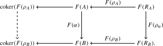
• An object $(A {\mathop {\longleftarrow }\limits ^{\rho _A}} R_A)$ in $\mathcal {A}(\mathbf {P})$ is mapped to ${{\,\mathrm{\mathrm {coker}}\,}}( F( \rho _A ) )$.

• Given a morphism

  $$\begin{aligned} \{\alpha , \rho _{\alpha }\}: (A {\mathop {\longleftarrow }\limits ^{\rho _A}} R_A) \longrightarrow (B {\mathop {\longleftarrow }\limits ^{\rho _B}} R_B) \in \mathcal {A}( \mathbf {P}), \end{aligned}$$

  we map it to the morphism induced by the universal property of the cokernels:

  

Correctness of the construction

The morphism induced by the universal property of the cokernel is independent of the morphism witness. Now, correctness follows from the functoriality of the cokernel. $\square$

Remark 3.21

If we have two operations ${{\,\mathrm{\mathrm {coker}}\,}}$, ${{\,\mathrm{\mathrm {coker}}\,}}'$ as instances of Construction 3.20.(3), then the corresponding induced functors U, $U'$ are naturally isomorphic.

4 Interpretations of Freyd Categories

In this subsection we want to give several classical interpretations of $\mathcal {A}( \mathbf {P})$ for specific inputs $\mathbf {P}$ that are all of the same spirit: the objects in $\mathcal {A}( \mathbf {P})$ represent finitely presented objects in some abelian category $\mathbf {A}$. The first theorem in this section is the main tool for giving these interpretations, and we will prove it classically (see Remark 2.3).

Theorem 4.1

(Stated and proven in classical mathematics) Let $\mathbf {P}$ be an additive category, $\mathbf {A}$ an abelian category, and $F: \mathbf {P}\rightarrow \mathbf {A}$ a full and faithful functor such that F(P) is a projective object for all $P \in \mathbf {P}$. Then the induced functor

$$\begin{aligned} U: \mathcal {A}( \mathbf {P}) \rightarrow \mathbf {A}\end{aligned}$$

is an equivalence between $\mathcal {A}( \mathbf {P})$ and the full subcategory $\mathbf {B}$ of $\mathbf {A}$ generated by those objects A for which there exist $P_A,Q_A \in \mathbf {P}$ and an exact sequence

$$\begin{aligned} 0 \longleftarrow A {\mathop {\longleftarrow }\limits ^{\epsilon _A}} F(P_A) {\mathop {\longleftarrow }\limits ^{\delta _A}} F(Q_A). \end{aligned}$$

Proof

We define an inverse functor $V: \mathbf {B}\rightarrow \mathcal {A}( \mathbf {P})$ as follows. We have an operation on objects sending $A \in \mathbf {B}$ to $(P_A {\mathop {\longleftarrow }\limits ^{d_A}} Q_A) \in \mathcal {A}( \mathbf {P})$, where $d_A$ is the preimage of $\delta _A$.

Let $B \in \mathbf {B}$ with $P_B, Q_B \in \mathbf {P}$ and $0 \longleftarrow B {\mathop {\longleftarrow }\limits ^{\epsilon _B}} F(P_B) {\mathop {\longleftarrow }\limits ^{\delta _B}} F(Q_B)$ exact. Using all of our assumptions on F, we can conclude: for $\alpha : A \rightarrow B \in \mathbf {B}$, there exists a morphism $p:P_A \rightarrow P_B$ such that

commutes for some morphism $q: Q_A \rightarrow Q_B$. Given another morphism $p': P_A \rightarrow P_B$ with this property, we have $(F(p) - F(p')) \cdot \epsilon _B = 0$. Again using all of our assumptions on F, we can conclude the existence of $\lambda : P_A \rightarrow Q_B$ such that $\lambda \cdot d_B = p - p'$, which proves that p and $p'$ are equal as morphisms from $(P_A {\mathop {\longleftarrow }\limits ^{d_A}} Q_A)$ to $(P_B {\mathop {\longleftarrow }\limits ^{d_B}} Q_B)$ in $\mathcal {A}( \mathbf {P})$. Thus, using the axiom of unique choice, $\alpha \mapsto p$ defines a well-defined action of V on morphisms. Furthermore, U and V are readily seen to be mutual inverses. $\square$

4.1 Finitely Presented Modules

Example 4.2

(Classical interpretation as finitely presented modules) Let R be a ring. We denote the abelian category of left R-modules by $R\text {-}\mathrm {Mod}$. We define $\mathrm {Rows}_R$ to be the full subcategory of $R\text {-}\mathrm {Mod}$ generated by all row modules $R^{1 \times n}$ for $n \in \mathbb {N}_0$ considered as free left modules. Morphisms ${{\,\mathrm{\mathrm {Hom}}\,}}_{\mathrm {Rows}_R}( R^{1 \times m}, R^{1 \times n} )$ can be naturally identified with matrices $R^{m \times n}$ for $m,n \in \mathbb {N}_0$. Then $\mathrm {Rows}_R \subseteq R\text {-}\mathrm {Mod}$ is a full and faithful embedding of projective objects. From Theorem 4.1 we conclude

$$\begin{aligned} \mathcal {A}( \mathrm {Rows}_R ) \simeq R\text {-}\mathrm {fpmod}, \end{aligned}$$

where $R\text {-}\mathrm {fpmod}$ is the category of finitely presented left R-modules.

The whole example also works for right modules by considering the full subcategory $\mathrm {Cols}_R \subseteq \mathrm {Mod}\text {-}R$ of right column modules instead. Note that if $M \in R^{n \times m}$ represents a morphism from $R^{m \times 1}$ to $R^{n \times 1}$ in $\mathrm {Cols}_R$, reinterpreting it as a morphism from $R^{1 \times n}$ to $R^{1 \times m}$ in $\mathrm {Rows}_R$ yields an equivalence $\mathrm {Cols}_R \simeq \mathrm {Rows}_R^{\mathrm {op}}$. Furthermore, $\mathrm {Rows}_R^{\mathrm {op}} \simeq \mathrm {Rows}_{R^{\mathrm {op}}}$. We conclude:

$$\begin{aligned} \mathcal {A}( \mathrm {Cols}_R ) \simeq \mathcal {A}( \mathrm {Rows}_R^{\mathrm {op}} ) \simeq \mathcal {A}( \mathrm {Rows}_{R^{\mathrm {op}}} ) \simeq \mathrm {fpmod}\text {-}R, \end{aligned}$$

where $\mathrm {fpmod}\text {-}R$ denotes the category of finitely presented right R-modules.

In [2] computable rings are introduced. We give a definition and a characterization of such rings using Freyd categories.

Definition 4.3

A ring R that

• (1) is left coherent, i.e., for a given matrix A with coefficients in R we can compute a matrix L such that $LA = 0$ and for all matrices T such that $TA = 0$, there exists a matrix U such that $UL = T$ (that means L generates the row syzygies),

• (2) has decidable lifts, i.e., there is an algorithm to decide solvability and to construct a particular solution of a linear system $XA = B$ for given matrices A, B with coefficients in R,

is called left computable. A ring R is right computable if $R^{\mathrm {op}}$ is left computable. If R is left and right computable, we simply call it computable.

Remark 4.4

Be aware of the existential quantifiers in Definition 4.3.(1). By our constructive interpretation we regard left coherent rings as being equipped with an algorithm for computing L (for given A) as well as U (for given A and T).

Remark 4.5

A left computable ring R has decidable equality, since $a = b$ if and only if $x\cdot 0 = (a-b)$ is solvable for $a,b \in R$ (and similar for right computable rings).

Theorem 4.6

Let R be a ring.

• (1) R is left coherent if and only if $\mathcal {A}( \mathrm {Rows}_R )$ is abelian.

• (2) R is left computable if and only if $\mathcal {A}( \mathrm {Rows}_R )$ is computable abelian.

Proof

R being left coherent is equivalent to $\mathrm {Rows}_R$ having weak kernels. So, the first claim follows from Theorem 3.5. R having decidable lifts is equivalent to $\mathrm {Rows}_R$ having decidable lifts, and the second claim follows from Corollary 3.18. $\square$

4.2 Finitely Presented Graded Modules

Example 4.7

(Classical interpretation as finitely presented graded modules) Let G be a group and S a G-graded ring, i.e., a ring with a direct sum decomposition $S = \bigoplus _{d \in G} S_d$ into abelian groups such that $S_{d} \cdot S_{e} \subseteq S_{d\cdot e}$ for all $d,e \in G$, and such that the multiplicative unit $1 \in S$ lies in $S_{e_G}$ with $e_G$ the neutral element of G. A graded left (resp. right) module is given by a left (resp. right) S-module M equipped with a direct sum decomposition $M = \bigoplus _{d \in G} M_d$ into abelian groups such that $S_d \cdot M_e \subseteq M_{d \cdot e}$ (resp. $M_e \cdot S_d \subseteq M_{e \cdot d})$ for all $d,e \in G$. Graded left (resp. right) S-module homomorphisms are given by left (resp. right) S-module homomorphisms respecting the grading. We denote the corresponding abelian category by $S\text {-}\mathrm {grMod}$ (resp. $\mathrm {grMod}\text {-}S$).

For a graded left (resp. right) module M and given $e \in G$, we denote by M(e) the e-th shift of M, i.e., the graded left module with $M(e)_d :=M_{d\cdot e}$ (resp. the graded right module with $M(e)_d :=M_{e\cdot d}$). The full subcategory generated by graded left (resp. right) modules of the form $S(e_1) \oplus \dots \oplus S(e_r)$ for $e_1, \dots , e_r \in G$, $r \in \mathbb {N}_0$ is denoted by $\mathrm {grRows}_S$ (resp. $\mathrm {grCols}_S$). Morphisms in $\mathrm {grRows}_S$ (resp. $\mathrm {grCols}_S$) from $S(d_1) \oplus \dots \oplus S(d_r)$ to $S(e_1) \oplus \dots \oplus S(e_s)$ for $d_1, \dots , d_r, e_1, \dots , e_s \in G$, $r,s \in \mathbb {N}_0$ can be naturally identified with matrices $H \in S^{r \times s}$ (resp. $H \in S^{s \times r}$) with homogeneous entries $H_{ij} \in S_{d_i^{-1} \cdot e_j}$ (resp. $H_{ji} \in S_{e_j \cdot d_i^{-1}}$) for $i=1, \dots ,r$, $j = 1,\dots , s$. Since $\mathrm {grRows}_S \subseteq S\text {-}\mathrm {grMod}$ (resp. $\mathrm {grCols}_S \subseteq \mathrm {grMod}\text {-}S$) are full and faithful embeddings of projective objects, we conclude (using Theorem 4.1)

$$\begin{aligned} \mathcal {A}(\mathrm {grRows}_S) \simeq S\text {-}\mathrm {fpgrmod}\text {~(resp.} ~ \mathcal {A}(\mathrm {grCols}_S) \simeq \mathrm {fpgrmod}\text {-}S) \end{aligned}$$

where $S\text {-}\mathrm {fpgrmod}$ (resp. $\mathrm {fpgrmod}\text {-}$ S) is the category of finitely presented graded left (resp. right) S-modules.

For an implementation of $\mathcal {A}(\mathrm {grRows}_S)$ as a computable abelian category, we need weak kernels and decidable lifts in $\mathrm {grRows}_S$ (Corollary 3.18). These requirements for $\mathrm {grRows}_S$ concisely encode the following specifications needed in an actual implementation: we need data structures for elements in G, a constructor for the neutral element $e_G \in G$, algorithms for multiplication, inversion, and equality in G. Furthermore, we need data structures for elements in $S_d$ ($d \in G$), constructors for $1 \in S_{e_G}$ and $0 \in S_d$ ($d \in G$), algorithms $S_d \times S_{d'} \rightarrow S_{dd'}$ for multiplication ($d,d' \in G$), algorithms $S_d \times S_{d} \rightarrow S_{d}$ for addition and subtraction ($d \in G$), and an algorithm for equality in $S_d$ $(d \in G)$. Furthermore, for weak kernels and decidable lifts in $\mathrm {grRows}_S$, we need an algorithm for computing homogeneous row syzygies of a matrix with homogeneous entries, and an algorithm for deciding the existence and in the affirmative case computing a solution of a linear system $X A = B$, where A, B and the solution X are matrices with homogeneous entries.

4.3 Finitely Presented Functors

We give a general interpretation of the Freyd category in terms of finitely presented functors (cf. [7, Corollary 3.9]).

Example 4.8

(Classical interpretation as finitely presented functors) Given an additive category $\mathbf {P}$, let

be the Yoneda embedding. Here, ${{\,\mathrm{\mathrm {Hom}}\,}}( \mathbf {P}^{\mathrm {op}}, \mathbf {Ab})$ denotes the abelian category of additive contravariant functors from $\mathbf {P}$ to the category of abelian groups $\mathbf {Ab}$, and $(-,P)$ denotes the contravariant ${{\,\mathrm{\mathrm {Hom}}\,}}$ functor. By Yoneda’s Lemma, is full and faithful. Again following from Yoneda’s Lemma, $(-,P)$ is a projective object. We conclude (using Theorem 4.1)

$$\begin{aligned} \mathcal {A}(\mathbf {P}) \simeq \mathrm {fp}( \mathbf {P}^{\mathrm {op}}, \mathbf {Ab}), \end{aligned}$$

where $\mathrm {fp}( \mathbf {P}^{\mathrm {op}}, \mathbf {Ab})$ is the category of contravariant finitely presented functors, i.e., the objects are functors $F: \mathbf {P}^{\mathrm {op}} \rightarrow \mathbf {Ab}$ for which there exists $A,B \in \mathbf {P}$ and an exact sequence of functors

and morphisms are given by natural transformations. Similarly, we get

$$\begin{aligned} \mathcal {A}(\mathbf {P}^{\mathrm {op}}) \simeq \mathrm {fp}( \mathbf {P}, \mathbf {Ab}), \end{aligned}$$

where $\mathrm {fp}( \mathbf {P}, \mathbf {Ab})$ is the category of covariant finitely presented functors, i.e., the full subcategory of the category of functors $F: \mathbf {P}\rightarrow \mathbf {Ab}$ for which there exists $A,B \in \mathbf {P}$ and an exact sequence of functors

We will study finitely presented functors in the case $\mathbf {P}$ abelian in Sect. 7.

5 Computationally Undecidable Lifting and Colifting Problems

In this section we provide several examples concerning computationally undecidable problems.

• 1. We give an example of a ring R with decidable equality⁸ whose lifting and colifting problems are computationally undecidable.

• 2. From such an R, we build a ring P with decidable equality whose colifting problem is still computationally undecidable, but now, P has decidable lifts.

• 3. We use P for the construction of an additive category $\mathbf {P}$ with decidable equality, having weak kernels, but whose lifting problem is computationally undecidable.

But first, we will explain what we mean by computationally undecidable problems.

Definition 5.1

Let $\mathbf {P}$ be an additive category. We say the lifting problem for $\mathbf {P}$ is computationally undecidable if $\mathbf {P}$ having decidable lifts would imply the decidability of a problem that is known to be undecidable by Turing machines. We proceed analogously for colifts.

Definition 5.2

Let R be a ring. We say the lifting problem for R is computationally undecidable if the lifting problem for $\mathrm {Rows}_R$ is computationally undecidable. We can rephrase this condition in terms of equations for R: having an algorithm for deciding and finding particular solutions of left-sided equations $XA = B$ for matrices A,B over R would imply the decidability of a problem that is known to be undecidable by Turing machines. We proceed analogously for colifts.

5.1 A Ring with Decidable Equality and Computationally Undecidable Lifting and Colifting Problem

We describe the famous word problem for finitely presented groups: given a finite set $\mathcal {X}$, let $\mathrm {Fr}(\mathcal {X})$ denote the free group over $\mathcal {X}$. Let furthermore $\mathcal {R}\subseteq \mathrm {Fr}(\mathcal {X})$ be a finite subset and N the normal subgroup generated by $\mathcal {R}$. The word problem for $H :=\mathrm {Fr}(\mathcal {X})/N$ (more precisely for $\mathcal {X}$ and $\mathcal {R}$) is the algorithmic problem of deciding if a given $w \in \mathrm {Fr}(\mathcal {X})$ represents the identity element in H, i.e., whether there is an algorithm rendering the (classically trivial⁹) proposition

$$\begin{aligned} \forall w \in \mathrm {Fr}(\mathcal {X}): (w \in N) \vee (w \not \in N) \end{aligned}$$

constructive. There are known concrete instances for $\mathcal {X}$ and $\mathcal {R}$ for which the word problem is undecidable [10] when we use Turing machines as a model of computation. Let $\mathcal {X},\mathcal {R}$ be such an instance.

Let $G :=\mathrm {Fr}(\mathcal {X}) \times \mathrm {Fr}(\mathcal {X})$ and let $M \subseteq G$ denote the equivalence relation induced on $\mathrm {Fr}(\mathcal {X})$ by N, i.e., the set of all pairs $(w_1, w_2)$ such that $w_1$ and $w_2$ represent the same element in H. Then M is the so-called Mihailova subgroup of G (introduced in [23]), and deciding whether $w \in \mathrm {Fr}(\mathcal {X})$ represents the identity in H is equivalent to deciding $(w,1) \in M$. It is easy to see that M is finitely generated as a subgroup by the finite set

$$\begin{aligned} M' :=\{ (x,x) \mid x \in \mathcal {X}\} \cup \{ (1,r) \mid r \in \mathcal {R}\}. \end{aligned}$$

We set $R :=k[G]$, i.e., R is the group ring of G with coefficients in a field with decidable equality¹⁰k. Then R is a k-algebra with decidable equality since the word problem in G is decidable. Furthermore, we claim that the lifting and colifting problems for R are computationally undecidable. This follows from the following lemma.

Lemma 5.3

Let k be a field, G be a group, and $M \subseteq G$ be a subgroup. We define the right ideal

$$\begin{aligned} I :=\langle 1 - m \mid m \in M \rangle _{k[G]} \end{aligned}$$

of the group ring k[G]. Given $g \in G$, we have

$$\begin{aligned} g \in M ~\Longleftrightarrow ~ (1 - g) \in I. \end{aligned}$$

Furthermore, if M is generated by the subset $M' \subseteq M$, then for the right ideal

$$\begin{aligned} I_{M'} :=\langle 1 - m' \mid m' \in M' \rangle _{k[G]}, \end{aligned}$$

we have

$$\begin{aligned} I = I_{M'}. \end{aligned}$$

Proof

Let $\epsilon : G \rightarrow M\backslash G$ be the canonical G-equivariant map from G into the set of right cosets of M in G. Then $\epsilon$ induces a map of right k[G]-modules

$$\begin{aligned} k[\epsilon ]: k[G] \rightarrow k[M\backslash G] \end{aligned}$$

with $I \subseteq {{\,\mathrm{\mathrm {ker}}\,}}(k[\epsilon ])$. If $(1-g) \in I$, then $k[\epsilon ](1-g) = 0 = M - Mg$, which gives $M = Mg$ and thus $g \in M$.

For the second claim, let $m_1,m_2 \in M$ such that $(1-m_1), (1-m_2) \in I_{M'}$. Then

$$\begin{aligned} (1 - m_1)(-m_1^{-1}) = 1 - m_1^{-1}\in I_{M'} \end{aligned}$$

and

$$\begin{aligned} (1-m_1)m_2 + (1-m_2) = 1 - m_1 m_2 \in I_{M'}. \end{aligned}$$

$\square$

Remark 5.4

The choice of formulating Lemma 5.3 in terms of right ideals was arbitrary. It is also valid with an analogous proof in terms of left ideals.

Corollary 5.5

The lifting and colifting problems are computationally undecidable for $k[\mathrm {Fr}(\mathcal {X}) \times \mathrm {Fr}(\mathcal {X})]$.

Proof

For $g \in \mathrm {Fr}(\mathcal {X}) \times \mathrm {Fr}(\mathcal {X})$ and $M'$ the finite generating set of the Mihailova subgroup, deciding whether $1-g$ lies in the finitely generated right ideal $I_{M'}$ is equivalent to deciding whether there exists a colift of the diagram

Analogously, checking whether an element lies in a finitely generated left ideal can be formulated in terms of a lifting problem. $\square$

5.2 A Ring with Decidable Equality, Decidable Lifts, and a Computationally Undecidable Colifting Problem

For simplifying our exposition, we axiomatize those properties of the ring R of the previous subsection that are needed for our construction in this subsection: let R be a k-algebra with decidable equality such that

• 1. R has an enumerable k-basis $v_1, v_2, v_3, \dots$,

• 2. the colifting problem for R is computationally undecidable.

The group ring $k[\mathrm {Fr}(\mathcal {X}) \times \mathrm {Fr}(\mathcal {X})]$ satisfies these requirements since

• 1. the elements of $\mathrm {Fr}(\mathcal {X}) \times \mathrm {Fr}(\mathcal {X})$ form a k-basis that can be enumerated,

• 2. the colifting problem for $k[\mathrm {Fr}(\mathcal {X}) \times \mathrm {Fr}(\mathcal {X})]$ is computationally undecidable due to Corollary 5.5.

Goal of this subsection the creation of a ring P with decidable equality, decidable lifts, and a computationally undecidable colifting problem.

The main idea: we create P from R by “adding” operators that help solving left-sided equations

$$\begin{aligned} X \cdot A = B \end{aligned}$$

(5.1)

for matrices A, B over R, but that are of no use for right-sided equations $A \cdot X = B$.

Helpful operators: as a k-vector space, we have $R = R^i \oplus \overline{R^i}$, where we set for $i \in \mathbb {N}$

• $R^i :=\langle v_1, \dots , v_i \rangle _k$,

• $\overline{R^i} :=\langle v_j \mid j > i \rangle _k$.

Given matrices A, B over R, there exists a $d \in \mathbb {N}$ such that all entries of A, B lie in $R^d$. If $(x_{mn})_{mn}$ is a solution over R for the left-sided Eq. (5.1), then each entry $x_{mn}$ could be replaced by a k-linear operator $\omega _{mn}$ in

$$\begin{aligned} \varOmega ^d :={{\,\mathrm{\mathrm {End}}\,}}_k( R^d ) \simeq k^{d \times d}, \end{aligned}$$

where $\omega _{mn}$ acts like $x_{mn}$ on $R^d$ and projects the result back into $R^d$. The crucial observation is the following: replacing the matrix $(x_{mn})_{mn}$ by $( \omega _{mn} )_{mn}$ still gives a solution for the left-sided Eq. (5.1).

Now, finding a solution of (5.1) with entries in $\varOmega ^d$ (where A and B are still defined over R) can be done by making an ansatz and using linear algebra. If no solution with entries in $\varOmega ^d$ exists, then there is also no solution with entries in R. This motivates to “add” the operator spaces $\varOmega ^i$ for all $i \in \mathbb {N}$ to R, but in an “unbalanced way”, i.e., the $\varOmega ^i$ must not be helpful for solving right-sided equations.

The details: we extend the action of an operator $\omega \in \varOmega ^i$ from $R^i$ to R by setting $\omega ( \overline{R^i} ) = 0$.

Construction 5.6

We construct a category $\mathbf {C}$ enriched over k as follows:

• 1. $\mathbf {C}$ consists of three objects that we denote by $z_1, z_2, z_3$.

• 2. The homomorphism k-vector spaces in $\mathbf {C}$ are determined by the following diagram:

  

  This means, ${{\,\mathrm{\mathrm {Hom}}\,}}_{\mathbf {C}}(z_1, z_2) = R \oplus \left( \bigoplus _{i \in \mathbb {N}} \varOmega ^i\right)$, ${{\,\mathrm{\mathrm {Hom}}\,}}_{\mathbf {C}}(z_2, z_3) = R$, ${{\,\mathrm{\mathrm {Hom}}\,}}(z_j, z_j) = k$ for $j = 1,2,3$, and ${{\,\mathrm{\mathrm {Hom}}\,}}_{\mathbf {C}}(z_1,z_3) = R$. The other ${{\,\mathrm{\mathrm {Hom}}\,}}$-sets are given by 0. Composition of two consecutive arrows $z_1 \rightarrow z_2$ and $z_2 \rightarrow z_3$ is induced by the operations of R and $\varOmega ^i$ on R.

Next, let P denote the path algebra of $\mathbf {C}$, i.e., its underlying vector space is

$$\begin{aligned} P = \bigoplus _{i=1}^3{{\,\mathrm{\mathrm {Hom}}\,}}_{\mathbf {C}}(z_i,z_i) \oplus {{\,\mathrm{\mathrm {Hom}}\,}}_{\mathbf {C}}(z_1,z_2) \oplus {{\,\mathrm{\mathrm {Hom}}\,}}_{\mathbf {C}}(z_2,z_3) \oplus {{\,\mathrm{\mathrm {Hom}}\,}}_{\mathbf {C}}(z_1,z_3) \end{aligned}$$

(5.2)

with multiplication given by composition in $\mathbf {C}$ and setting the multiplication of two non-composable morphisms to 0. Then P has decidable equality.

Given an element $x \in P$, we will write

$$\begin{aligned} x = x^{(1,1)} + x^{(2,2)} + x^{(3,3)} + x^{(1,2)} + x^{(2,3)} + x^{(1,3)} \end{aligned}$$

for its decomposition w.r.t. the direct sum decomposition (5.2).

Lemma 5.7

The colifting problem is computationally undecidable for P.

Proof

We reduce the computationally undecidable colifting problem of R to the colifting problem of P. Given matrices A, B over R, we interpret the entries of A as elements in ${{\,\mathrm{\mathrm {Hom}}\,}}_{\mathbf {C}}( z_1, z_2 )$ and the entries in B as elements in ${{\,\mathrm{\mathrm {Hom}}\,}}_{\mathbf {C}}(z_1,z_3)$. Then $A \cdot X = B$ has a solution over R if and only if it has a solution over P, since a solution over R can be interpreted as a solution with entries in ${{\,\mathrm{\mathrm {Hom}}\,}}_{\mathbf {C}}(z_2,z_3) \subseteq P$, and a solution $X = (x_{mn})_{mn}$ over P gives rise to a solution $(x_{mn}^{(2,3)})_{mn}$ with entries in ${{\,\mathrm{\mathrm {Hom}}\,}}_{\mathbf {C}}(z_2,z_3) = R$. $\square$

For the proof of the next lemma, we introduce the following spaces for all $i \in \mathbb {N}$:

• ${{\,\mathrm{\mathrm {Hom}}\,}}_{\mathbf {C}}^i(z_1,z_2) :=R^i \oplus (\bigoplus _{j \le i} \varOmega ^j) \subseteq {{\,\mathrm{\mathrm {Hom}}\,}}_{\mathbf {C}}(z_1,z_2)$

• $\overline{{{\,\mathrm{\mathrm {Hom}}\,}}_{\mathbf {C}}^i}(z_1,z_2) :=\overline{R^i} \oplus (\bigoplus _{j > i} \varOmega ^j) \subseteq {{\,\mathrm{\mathrm {Hom}}\,}}_{\mathbf {C}}(z_1,z_2)$

• ${{\,\mathrm{\mathrm {Hom}}\,}}_{\mathbf {C}}^i(z_m,z_n) :=R^i \subseteq {{\,\mathrm{\mathrm {Hom}}\,}}_{\mathbf {C}}(z_m,z_n)$ for $(m,n) \in \{(1,3),(2,3)\}$

• $\overline{{{\,\mathrm{\mathrm {Hom}}\,}}_{\mathbf {C}}^i}(z_m,z_n) :=\overline{R^i} \subseteq {{\,\mathrm{\mathrm {Hom}}\,}}_{\mathbf {C}}(z_m,z_n)$ for $(m,n) \in \{(1,3),(2,3)\}$

• $P^i :=\bigoplus _{i=1}^3{{\,\mathrm{\mathrm {Hom}}\,}}_{\mathbf {C}}(z_i,z_i) \oplus {{\,\mathrm{\mathrm {Hom}}\,}}_{\mathbf {C}}^i(z_1,z_2) \oplus {{\,\mathrm{\mathrm {Hom}}\,}}_{\mathbf {C}}^i(z_2,z_3) \oplus {{\,\mathrm{\mathrm {Hom}}\,}}_{\mathbf {C}}^i(z_1,z_3)$

• $\overline{P^i} :=\overline{{{\,\mathrm{\mathrm {Hom}}\,}}_{\mathbf {C}}^i}(z_1,z_2) \oplus \overline{{{\,\mathrm{\mathrm {Hom}}\,}}_{\mathbf {C}}^i}(z_2,z_3) \oplus \overline{{{\,\mathrm{\mathrm {Hom}}\,}}_{\mathbf {C}}^i}(z_1,z_3)$

Given an element $x \in P$, we will write

$$\begin{aligned} x = x^i + \overline{x^i} \end{aligned}$$

for its decomposition in $P^i \oplus \overline{P^i}$.

Theorem 5.8

P has decidable lifts.

Proof

Given matrices A, B over P, we need to decide whether there exists a matrix X over P such that $X \cdot A = B$, and in the affirmative case construct such a matrix. There exist $d, d' \in \mathbb {N}$ such that all entries of A and B lie in $P^d$ and such that such that $R^d \cdot R^d \subseteq R^{d'}$ (which is actually equivalent to $P^d \cdot P^d \subseteq P^{d'}$). Our main claim is the following:

Once we know that our main claim is true, $X \cdot A = B$ can simply be solved by making an ansatz with all entries of X lying in $P^{d'}$. This ansatz yields a linear system over k and can be dealt with since k is a field with decidable equality.

The “only if” direction of our main claim is the hard part, so let us assume that we are given a solution X over P. We define an operator $\sigma : P \rightarrow P^{d'}$ with the idea that entrywise applied to X it will also yield a solution:

$$\begin{aligned} \sigma (x) :=x^d + \tau ( \overline{x^d} ), \end{aligned}$$

where we define

$$\begin{aligned} \tau : \overline{P^d}&\rightarrow P^{d'}: \\ \overline{{{\,\mathrm{\mathrm {Hom}}\,}}_{\mathbf {C}}^d(z_1,z_2)} \ni p&\mapsto \left( \tau (p):R^{d'} \rightarrow R^{d'}: y \mapsto (p \cdot y)^{d'}\right) \\ \overline{{{\,\mathrm{\mathrm {Hom}}\,}}_{\mathbf {C}}^d(z_2,z_3)} \ni q&\mapsto 0 \\ \overline{{{\,\mathrm{\mathrm {Hom}}\,}}_{\mathbf {C}}^d(z_1,z_3)} \ni r&\mapsto r^{d'} \end{aligned}$$

Here, $\tau (p)$ denotes the operator in $\varOmega ^{d'} \subseteq {{\,\mathrm{\mathrm {Hom}}\,}}_{\mathbf {C}}(z_1,z_2)$ that maps $y \in R^{d'} \subseteq {{\,\mathrm{\mathrm {Hom}}\,}}_{\mathbf {C}}(z_2,z_3)$ to $(p \cdot y)^{d'} \in R^{d'} \subseteq {{\,\mathrm{\mathrm {Hom}}\,}}_{\mathbf {C}}(z_1,z_3)$.

We show that $\sigma$ entrywise applied to X yields a solution: given $x_1, \dots , x_n \in P$ and $a_1, \dots , a_n \in P^d$ for $n \in \mathbb {N}_0$ such that $\sum _{i=1}^nx_i \cdot a_i \in P^d$, we claim that

$$\begin{aligned} \sum _{i=1}^nx_i \cdot a_i = \sum _{i=1}^n \sigma (x_i) \cdot a_i. \end{aligned}$$

For this, it suffices to show that

$$\begin{aligned} \sum _{i=1}^n \overline{x_i^d} \cdot a_i = \sum _{i=1}^n \tau (\overline{x_i^d}) \cdot a_i. \end{aligned}$$

(5.3)

Due to our choice of $d'$, the term $\sum _{i=1}^n \overline{x_i^d} \cdot a_i = \sum _{i=1}^n x_i \cdot a_i - \sum _{i=1}^n x_i^d \cdot a_i$ lies in

$$\begin{aligned} P^d \cdot P^d \subseteq \bigoplus _{i=1}^3{{\,\mathrm{\mathrm {Hom}}\,}}_{\mathbf {C}}(z_i,z_i) \oplus {{\,\mathrm{\mathrm {Hom}}\,}}_{\mathbf {C}}^d(z_1,z_2) \oplus {{\,\mathrm{\mathrm {Hom}}\,}}_{\mathbf {C}}^d(z_2,z_3) \oplus {{\,\mathrm{\mathrm {Hom}}\,}}_{\mathbf {C}}^{d'}(z_1,z_3). \end{aligned}$$

(5.4)

Now, to simplify our notation, we write

$$\begin{aligned} \overline{x_i^d} = p_i + q_i + r_i \in \overline{{{\,\mathrm{\mathrm {Hom}}\,}}_{\mathbf {C}}^d}(z_1,z_2) \oplus \overline{{{\,\mathrm{\mathrm {Hom}}\,}}_{\mathbf {C}}^d}(z_2,z_3) \oplus \overline{{{\,\mathrm{\mathrm {Hom}}\,}}_{\mathbf {C}}^d}(z_1,z_3) \end{aligned}$$

for the decomposition of $\overline{x_i^d}$ w.r.t. the above direct sum. Rewriting the claim 5.3 gives

$$\begin{aligned} \sum _{i=1}^n (p_i + q_i + r_i) \cdot a_i = \sum _{i=1}^n (\tau (p_i) + r_i^{d'} ) \cdot a_i. \end{aligned}$$

(5.5)

We have

$$\begin{aligned} \sum _{i=1}^n q_i \cdot a_i = 0, \end{aligned}$$

since

$$\begin{aligned} \sum _{i=1}^n q_i \cdot a_i = \sum _{i=1}^n q_i \cdot a_i^{(3,3)} \end{aligned}$$

both lies in $\overline{{{\,\mathrm{\mathrm {Hom}}\,}}_{\mathbf {C}}(z_2,z_3)^d}$ (since the $a_i^{(3,3)}$ act like scalars) and ${{\,\mathrm{\mathrm {Hom}}\,}}_{\mathbf {C}}(z_2,z_3)^d$ [due to (5.4)]. Thus, the claim (5.5) simplifies to

$$\begin{aligned} \sum _{i=1}^n (p_i + r_i) \cdot a_i = \sum _{i=1}^n (\tau (p_i) + r_i^{d'} ) \cdot a_i, \end{aligned}$$

which is equivalent to

$$\begin{aligned} \sum _{i=1}^n (p_i + r_i) \cdot (a_i^{(2,2)} + a_i^{(2,3)} + a_i^{(3,3)}) = \sum _{i=1}^n (\tau (p_i) + r_i^{d'} ) \cdot (a_i^{(2,2)} + a_i^{(2,3)} + a_i^{(3,3)}), \end{aligned}$$

which in turn is equivalent to the two equations

$$\begin{aligned} \sum _{i=1}^n p_i\cdot a_i^{(2,2)} = \sum _{i=1}^n \tau (p_i)\cdot a_i^{(2,2)} \end{aligned}$$

(5.6)

and

$$\begin{aligned} \sum _{i=1}^n p_i\cdot a_i^{(2,3)} + r_i\cdot a_i^{(3,3)} = \sum _{i=1}^n \tau (p_i)\cdot a_i^{(2,3)} + r_i^{d'}\cdot a_i^{(3,3)}. \end{aligned}$$

(5.7)

First, we deal with (5.6):

$$\begin{aligned} \sum _{i=1}^n p_i\cdot a_i^{(2,2)} = 0 \end{aligned}$$

since this term both lies in $\overline{{{\,\mathrm{\mathrm {Hom}}\,}}_{\mathbf {C}}(z_1,z_2)^d}$ (since the $a_i^{(2,2)}$ act like scalars) and ${{\,\mathrm{\mathrm {Hom}}\,}}_{\mathbf {C}}(z_1,z_2)^d$ [due to (5.4)]. Because $\tau$ is a linear map, we also have

$$\begin{aligned} \sum _{i=1}^n \tau (p_i)\cdot a_i^{(2,2)} = 0. \end{aligned}$$

Finally, we deal with (5.7):

$$\begin{aligned} \sum _{i=1}^n p_i\cdot a_i^{(2,3)} + r_i\cdot a_i^{(3,3)}&= \left( \sum _{i=1}^n p_i\cdot a_i^{(2,3)} + r_i\cdot a_i^{(3,3)}\right) ^{d'}&\text {(due to }(5.4)\mathrm{)} \\&= \sum _{i=1}^n (p_i\cdot a_i^{(2,3)})^{d'} + r_i^{d'}\cdot a_i^{(3,3)}&\text {(linearity)} \\&= \sum _{i=1}^n \tau (p_i)\cdot a_i^{(2,3)} + r_i^{d'}\cdot a_i^{(3,3)}&\text {(definition of } \tau ). \end{aligned}$$

$\square$

5.3 An Additive Category with Decidable Equality, Having Kernels, and a Computationally Undecidable Lifting Problem

Let P be the ring constructed in Sect. 5.2. It has decidable lifts but a computationally undecidable colifting problem. Set $\mathbf {P}:=\mathcal {A}( \mathrm {Rows}_{P} )^{\mathrm {op}}$. Then $\mathbf {P}$ is additive with decidable equality, since P has decidable lifts. Furthermore it has weak kernels (even kernels), since $\mathcal {A}( \mathrm {Rows}_{P} )$ has cokernels by Construction 3.6.

However, the lifting problem for $\mathbf {P}$ is computationally undecidable: an algorithm for deciding lifts in $\mathbf {P}= \mathcal {A}( \mathrm {Rows}_{P} )^{\mathrm {op}}$, i.e., colifts in $\mathcal {A}( \mathrm {Rows}_{P} )$, immediately gives an algorithm for deciding colifts in $\mathrm {Rows}_{P}$ (because $\mathrm {Rows}_{P} \subseteq \mathcal {A}( \mathrm {Rows}_{P} )$ is a full embedding). But the colifting problem is computationally undecidable for P by Lemma 5.7. We have proven the main theorem of this section:

Theorem 5.9

The category $\mathcal {A}(\mathrm {Rows}_{P})^{\mathrm {op}}$ is additive with decidable equality, has kernels, but its lifting problem is computationally undecidable.

Remark 5.10

Theorem 5.9 shows that even if we have an additive category with decidable equality and weak kernels (this includes having an algorithm for lifting those cospans representing a test situation for the weak kernel), we cannot expect to derive an algorithm for solving the lifting problem from these data.

Remark 5.11

$\mathcal {A}(\mathcal {A}(\mathrm {Rows}_{P})^{\mathrm {op}})$ is abelian by Theorem 3.5. However, $\mathcal {A}(\mathcal {A}(\mathrm {Rows}_{P})^{\mathrm {op}})$ being computable abelian implies P having decidable colifts, which is a computationally undecidable problem. This behavior is not uncommon in our constructive setup. Another example of such an abelian category is the category of unbounded chain complexes of finite dimensional k-vector spaces for a field k with decidable equality.

6 Lifts and Homomorphism Structures

We are going to address the problem of computing lifts in the Freyd category $\mathcal {A}(\mathbf {P})$ for an additive category $\mathbf {P}$. To this end, we take a look at the following diagram:

The solid arrows represent given morphisms in $\mathcal {A}(\mathbf {P})$, the dashed morphism $\{X,Y\}$ in $\mathcal {A}(\mathbf {P})$ is the lift which we want to compute (with unknowns X, Y), i.e., it has to satisfy

$$\begin{aligned} \rho _A \cdot X = Y \cdot \rho _C \end{aligned}$$

(6.1)

for being well-defined and

$$\begin{aligned} X \cdot \gamma - \alpha = Z \cdot \rho _B \end{aligned}$$

(6.2)

for being a lift, where the unknown Z is a witness for $\alpha$ and $X \cdot \gamma$ being equal. Thus, computing a lift in $\mathcal {A}(\mathbf {P})$ means finding morphisms X, Y, Z in $\mathbf {P}$ satisfying Eqs. (6.1) and (6.2).

6.1 Linear Systems in Additive Categories

In order to develop a strategy for solving Eqs. (6.1) and (6.2), we discuss arbitrary linear systems in $\mathbf {P}$.

Definition 6.1

Let $\mathbf {P}$ be an additive category. A linear system in $\mathbf {P}$ with $m \in \mathbb {N}$ equations in $n \in \mathbb {N}$ indeterminates is defined by the following data:

• 1. Objects $(A_i)_i, (D_i)_i$ and $(B_j)_j, (C_j)_j$ in $\mathbf {P}$ for $i = 1, \dots , m$, $j = 1, \dots , n$.

• 2. Morphisms $(\alpha _{ij}: A_i \rightarrow B_j)_{ij}$ and $(\beta _{ij}: C_j \rightarrow D_i)_{ij}$ in $\mathbf {P}$ for $i = 1, \dots , m$, $j = 1, \dots , n$.

• 3. Morphisms $(\gamma _i: A_i \rightarrow D_i)_i$ in $\mathbf {P}$ for $i = 1, \dots , m$.

A solution is given by morphisms $(X_j: B_j \rightarrow C_j)_{j=1,\dots ,n}$ such that the equations

$$\begin{aligned} \begin{array}{ccccccccc} \alpha _{11} \cdot X_1 \cdot \beta _{11} &{}+&{} \alpha _{12} \cdot X_2 \cdot \beta _{12} &{}+&{} \dots &{}+&{} \alpha _{1n} \cdot X_n \cdot \beta _{1n} &{}=&{} \gamma _1 \\ \vdots &{} &{} \vdots &{} &{} \vdots &{} &{} \vdots &{} &{}\vdots \\ \alpha _{m1} \cdot X_1 \cdot \beta _{m1} &{}+&{} \alpha _{m2} \cdot X_2 \cdot \beta _{m2} &{}+&{} \dots &{}+&{} \alpha _{mn} \cdot X_n \cdot \beta _{mn} &{}=&{} \gamma _m \\ \end{array} \end{aligned}$$

hold. We say $\mathbf {P}$ has decidable linear systems if we have an algorithm that constructs for a given linear system a solution or disproves its existence.

Definition 6.2

Let $\mathbf {P}$ be an additive category. The set of iterated Freyd categories of $\mathbf {P}$ is defined inductively:

• 1. $\mathbf {P}$ is an iterated Freyd category of $\mathbf {P}$.

• 2. If $\mathbf {X}$ is an iterated Freyd category of $\mathbf {P}$, then so are $\mathbf {X}^{\mathrm {op}}$ and $\mathcal {A}( \mathbf {X})$.

Important examples of iterated Freyd categories are $\mathcal {A}( \mathcal {A}( \mathbf {P}) )$ and $\mathcal {A}( \mathcal {A}( \mathbf {P})^{\mathrm {op}} )$ (see Example 4.8). The next theorem is a generalization of the discussion in the beginning of this section.

Theorem 6.3

Let $\mathbf {P}$ be an additive category. Any linear system in an iterated Freyd category $\mathbf {X}$ of $\mathbf {P}$ gives rise to a linear system in $\mathbf {P}$ such that the former has a solution if and only if the latter has a solution.

Proof by induction

The case $\mathbf {X}= \mathbf {P}$ is trivial. Furthermore, any linear system in $\mathbf {X}^{\mathrm {op}}$ trivially gives rise to an equivalent linear system in $\mathbf {X}$. So, let

$$\begin{aligned} \begin{array}{ccc} \sum _{j=1}^n \{\alpha _{1j}, \rho _{\alpha _{1j}} \} \cdot X_j \cdot \{ \beta _{1j}, \rho _{\beta _{1j}} \} &{}=&{} \{\gamma _1, \rho _{\gamma _1} \} \\ \vdots &{} &{}\vdots \\ \sum _{j=1}^n \{\alpha _{mj}, \rho _{\alpha _{mj}} \} \cdot X_j \cdot \{\beta _{mj}, \rho _{\beta _{mj}}\} &{}=&{} \{\gamma _m, \rho _{\gamma _m} \}\\ \end{array} \end{aligned}$$

be a linear system in $\mathcal {A}( \mathbf {X})$, where the corresponding sources and ranges are denoted by

• $\{\alpha _{ij}, \rho _{\alpha _{ij}}\}: (A_i {\mathop {\longleftarrow }\limits ^{\rho _{A_i}}} R_{A_i}) \longrightarrow (B_j {\mathop {\longleftarrow }\limits ^{\rho _{B_j}}} R_{B_j})$,

• $\{\beta _{ij}, \rho _{\beta _{ij}}\}: (C_j {\mathop {\longleftarrow }\limits ^{\rho _{C_j}}} R_{C_j}) \longrightarrow (D_i {\mathop {\longleftarrow }\limits ^{\rho _{D_i}}} R_{D_i})$,

• $\{\gamma _{i}, \rho _{\gamma _{i}}\}: (A_i {\mathop {\longleftarrow }\limits ^{\rho _{A_i}}} R_{A_i}) \longrightarrow (D_i {\mathop {\longleftarrow }\limits ^{\rho _{D_i}}} R_{D_i})$.

To define an equivalent linear system in $\mathbf {X}$, we introduce variables $(X_j^1)_j$, $(X_j^2)_j$, and the set of linear equations

$$\begin{aligned} X_j^2 \cdot \rho _{C_j} = \rho _{B_j} \cdot X_j^1 \end{aligned}$$

encoding well-definedness of $\{X_j^1, X_j^2\}: (B_j {\mathop {\longleftarrow }\limits ^{\rho _{B_j}}} R_{B_j}) \longrightarrow (C_j {\mathop {\longleftarrow }\limits ^{\rho _{C_j}}} R_{C_j})$. Furthermore, for each original equation, we need a “witness-variable” $(Z_i: A_i \rightarrow R_{D_i})_i$. Now, we can simply encode the original equations by the following linear equations in $\mathbf {X}$:

$$\begin{aligned} \begin{array}{ccc} \sum _{j=1}^n \alpha _{1j} \cdot X_j^1 \cdot \beta _{1j} &{}=&{} \gamma _1 + Z_1 \cdot \rho _{D_1} \\ \vdots &{} &{}\vdots \\ \sum _{j=1}^n \alpha _{mj} \cdot X_j^1 \cdot \beta _{mj} &{}=&{} \gamma _m + Z_m \cdot \rho _{D_m}. \end{array} \end{aligned}$$

$\square$

Key observation: finding a solution of a linear system in $\mathbf {P}$ is equivalent to finding a lift of the following diagram of abelian groups:

The data needed to form this diagram are

• 1. the abelian group $\mathbb {Z}$,

• 2. the ${{\,\mathrm{\mathrm {Hom}}\,}}$-functor of $\mathbf {P}$ mapping to the category of abelian groups,

• 3. the translation of elements in ${{\,\mathrm{\mathrm {Hom}}\,}}_{\mathbf {P}}(A,B)$ to morphisms $\mathbb {Z}\rightarrow {{\,\mathrm{\mathrm {Hom}}\,}}_{\mathbf {P}}(A,B)$.

We abstract these data in the following definition¹¹.

Definition 6.4

Let $\mathbf {P}$, $\mathbf {B}$ be additive categories. A $\mathbf {B}$-homomorphism structure for $\mathbf {P}$ consists of the following data:

• 1. A distinguished object $1 \in \mathbf {B}$.

• 2. A bilinear functor $H: \mathbf {P}^{\mathrm {op}} \times \mathbf {P}\rightarrow \mathbf {B}$, i.e., a functor which is additive in each component.

• 3. An isomorphism $\nu : {{\,\mathrm{\mathrm {Hom}}\,}}_{\mathbf {P}}( P, Q ) \xrightarrow {\sim } {{\,\mathrm{\mathrm {Hom}}\,}}_{\mathbf {B}}( 1, H( P, Q ) )$ natural in $P,Q \in \mathbf {P}$, i.e, $\nu ( \alpha \cdot X \cdot \beta ) = \nu ( X ) \cdot H(\alpha , \beta )$ for all composable triples of morphisms $\alpha , X, \beta$.

Remark 6.5

The definition of a homomorphism structure is related to enriched category theory in the following way: whenever we have a category $\mathbf {P}$ enriched over a locally small symmetric monoidal closed category $\mathbf {B}$, let $H(P,Q) \in \mathbf {B}$ denote the hom object of $P, Q \in \mathbf {P}$. Let $\mathbf {P}_0$ denote the underlying category of $\mathbf {P}$, i.e., the category whose objects are the objects of $\mathbf {P}$, and ${{\,\mathrm{\mathrm {Hom}}\,}}_{\mathbf {P}_0}( P, Q ) = {{\,\mathrm{\mathrm {Hom}}\,}}_{\mathbf {B}}( 1, H( P, Q ) )$, where 1 denotes the tensor unit of $\mathbf {B}$. Then the family of hom objects gives rise to a functor $H: \mathbf {P}_0^{\mathrm {op}} \times \mathbf {P}_0 \rightarrow \mathbf {B}$ such that ${{\,\mathrm{\mathrm {Hom}}\,}}_{\mathbf {P}_0}( P, Q ) \xrightarrow {\sim } {{\,\mathrm{\mathrm {Hom}}\,}}_{\mathbf {B}}( 1, H( P, Q ) )$ natural in P, Q (see [21, Section 1.6]).

Example 6.6

We use the notation of Example 4.2. Let R be a commutative ring. The functor

$$\begin{aligned} H: \mathrm {Rows}_R^{\mathrm {op}} \times \mathrm {Rows}_R&\longrightarrow \mathrm {Rows}_{R}: \\ (R^{1 \times a} {\mathop {\longleftarrow }\limits ^{A}} R^{1 \times a'}, R^{1 \times b} {\mathop {\longrightarrow }\limits ^{B}} R^{1 \times b'})&\longmapsto \big (A_{ij}B_{kl}\big )_{ijkl}: \bigoplus _{j=1}^{a}\bigoplus _{k=1}^{b}{R^{1 \times 1}} \longrightarrow \bigoplus _{i=1}^{a'}\bigoplus _{l=1}^{b'}{R^{1 \times 1}} \end{aligned}$$

defines a $\mathrm {Rows}_R$-homomorphism structure for $\mathrm {Rows}_R$ with distinguished object $R^{1 \times 1}$ and the natural isomorphism of R-modules

$$\begin{aligned}{{\,\mathrm{\mathrm {Hom}}\,}}_{\mathrm {Rows}_R}( R^{1 \times a}, R^{1 \times b} ) \simeq _R {{\,\mathrm{\mathrm {Hom}}\,}}_{\mathrm {Rows}_R}( R^{1 \times 1}, \bigoplus _{j=1}^{a}\bigoplus _{k=1}^{b}{R^{1 \times 1}} ).\end{aligned}$$

Note that H can be interpreted as the restriction of the ${{\,\mathrm{\mathrm {Hom}}\,}}$-functor of $R\text {-}\mathrm {Mod}$ to row modules.

The previous example only worked due to the commutativity of the ring in question. In the next example we show what we can do in the non-commutative case provided that the center of the ring is “big enough”.

Example 6.7

We use the notation of Example 4.2. Let R be a ring and $C \subseteq R$ its center. Assume that R is finitely presented as a C-module, i.e., there exists an exact sequence of C-modules

for $a,b \in \mathbb {N}$, where ${_{C}R}$ denotes R regarded as a C-module. In this case the ${{\,\mathrm{\mathrm {Hom}}\,}}$-functor for $\mathrm {Rows}_R$ can be seen as a functor mapping to $C\text {-}\mathrm {fpmod}$:

$$\begin{aligned} \mathrm {Rows}_R^{\mathrm {op}} \times \mathrm {Rows}_R&\longrightarrow C\text {-}\mathrm {fpmod}: \\ (R^{1 \times c}, R^{1 \times d})&\longmapsto {{\,\mathrm{\mathrm {Hom}}\,}}_R( R^{1 \times c}, R^{1 \times d}) \simeq {_{C}R}^{1 \times cd} \end{aligned}$$

This gives rise to a $C\text {-}\mathrm {fpmod}$-homomorphism structure for $\mathrm {Rows}_R$ with distinguished object $C^{1 \times 1} \in C\text {-}\mathrm {fpmod}$ and natural isomorphism

$$\begin{aligned}{{\,\mathrm{\mathrm {Hom}}\,}}_{\mathrm {Rows}_R}( R^{1 \times c}, R^{1 \times d}) \simeq _C {{\,\mathrm{\mathrm {Hom}}\,}}_{C\text {-}\mathrm {fpmod}}\left( C^{1\times 1}, {_{C}R}^{1 \times cd} \right) \end{aligned}$$

induced by the natural bijection between elements in R and C-module homomorphisms from C to ${_{C}R}$. This homomorphism structure transfers to a $\mathcal {A}( \mathrm {Rows}_C )$-homomorphism structure via the equivalence $C\text {-}\mathrm {fpmod}\simeq \mathcal {A}( \mathrm {Rows}_C )$ (see Example 4.2).

Example 6.8

If $\mathbf {P}$ is an additive closed symmetric monoidal category, then its tensor unit $1 \in \mathbf {P}$ and the internal ${{\,\mathrm{\mathrm {Hom}}\,}}$-functor define a $\mathbf {P}$-homomorphism structure for $\mathbf {P}$.

Example 6.9

If $(1,H: \mathbf {P}^{\mathrm {op}} \times \mathbf {P}\rightarrow \mathbf {B},\nu )$ is a $\mathbf {B}$-homomorphism structure for $\mathbf {P}$, then swapping components $G: \mathbf {P}\times \mathbf {P}^{\mathrm {op}} \xrightarrow {\sim } \mathbf {P}^{\mathrm {op}} \times \mathbf {P}{\mathop {\longrightarrow }\limits ^{H}} \mathbf {B}$ defines a $\mathbf {B}$-homomorphism structure for $\mathbf {P}^{\mathrm {op}}$ with distinguished object 1.

The following theorem is an abstraction of a computational trick presented in [31] (see also [5]).

Theorem 6.10

We use the notation of Definition 6.1. Let $\mathbf {P}$ be an additive category equipped with a $\mathbf {B}$-homomorphism structure $(1, H, \nu )$. Given a linear system in $\mathbf {P}$, then $(X_j)_j$ is a solution if and only if it gives rise to a lift of the following diagram in $\mathbf {B}$:

Proof

We compute

$$\begin{aligned} ( \nu (X_j) )_j \cdot ( H( \alpha _{ij}, \beta _{ij} ) )_{ji}&= ( \sum _j \nu (X_j) \cdot H( \alpha _{ij}, \beta _{ij} ) )_i&\text {matrix multiplication} \\&= ( \sum _j \nu ( \alpha _{ij} \cdot X_j \cdot \beta _{ij} ) )_i&\text {naturality of } \nu \\&= ( \nu ( \sum _j \alpha _{ij} \cdot X_j \cdot \beta _{ij} ) )_i&\text {linearity of } \nu \end{aligned}$$

Since $\nu$ is an isomorphism, the last term equals $(\nu (\gamma _i))_i$ if and only if $(X_j)_j$ is a solution. $\square$

Corollary 6.11

Let $\mathbf {P}$ be an additive category equipped with a $\mathbf {B}$-homomorphism structure $(1, H, \nu )$. If $\mathbf {B}$ has decidable lifts, then $\mathbf {P}$ has decidable linear systems. In particular, if $\mathbf {B}$ has decidable lifts, then any iterated Freyd category of $\mathbf {P}$ has decidable linear systems.

Proof

We use Theorems 6.3 and 6.10. $\square$

Example 6.12

Let R be a commutative ring. Then $\mathrm {Rows}_R$ has a $\mathrm {Rows}_R$-homomorphism structure (Example 6.6). If R has decidable lifts, then $\mathcal {A}( \mathrm {Rows}_R )$ and all the other iterated Freyd categories of $\mathrm {Rows}_R$ have decidable linear systems (in particular lifts and colifts) (Corollary 6.11).

Using the previous example, we can deal with more general rings:

Example 6.13

Let R be a ring that is finitely presented as a module over its center. Then $\mathrm {Rows}_R$ has an $\mathcal {A}( \mathrm {Rows}_C )$-homomorphism structure (Example 6.7). If C has decidable lifts, then so does $\mathcal {A}( \mathrm {Rows}_C )$ (Example 6.12). It follows that $\mathcal {A}( \mathrm {Rows}_R )$ and all the other iterated Freyd categories of $\mathrm {Rows}_R$ have decidable linear systems (in particular lifts and colifts) (Corollary 6.11).

6.2 Homomorphism Structures in Freyd Categories

We show that certain $\mathbf {B}$-homomorphism structures for $\mathbf {P}$ induce $\mathbf {B}$-homomorphism structures for $\mathcal {A}(\mathbf {P})$. We will use such an induced homomorphism structure in Sect. 7.2 to compute the sets of natural transformations between finitely presented functors.

Construction 6.14

Let $\mathbf {P}$ be an additive category, $\mathbf {B}$ an abelian category. Furthermore, let $H: \mathbf {P}^{\mathrm {op}} \times \mathbf {P}\rightarrow \mathbf {B}$ be a bilinear functor. We want to construct from these data a bilinear functor

$$\begin{aligned} H^{\mathcal {A}}: \mathcal {A}(\mathbf {P})^{\mathrm {op}} \times \mathcal {A}( \mathbf {P}) \longrightarrow \mathbf {B}\end{aligned}$$

extending H (where we think of $\mathbf {P}$ as a full subcategory of $\mathcal {A}( \mathbf {P})$). Given morphisms

$$\begin{aligned}\{\alpha , \rho _{\alpha }\}: (A' {\mathop {\longleftarrow }\limits ^{\rho _{A'}}} R_{A'}) \longrightarrow (A {\mathop {\longleftarrow }\limits ^{\rho _A}} R_A)\end{aligned}$$

and

$$\begin{aligned}\{\beta , \rho _{\beta }\}: (B {\mathop {\longleftarrow }\limits ^{\rho _B}} R_B) \longrightarrow (B' {\mathop {\longleftarrow }\limits ^{\rho _{B'}}} R_{B'})\end{aligned}$$

in $\mathcal {A}(\mathbf {P})$, we set $H^{\mathcal {A}}( \{\alpha , \rho _{\alpha }\}, \{\beta , \rho _{\beta }\} )$ as the morphism between the kernels in the diagram

where we overline a morphism to address its induced morphism on quotient objects.

Correctness of the construction

To see that all four overlined morphisms in the right square are well-defined, let us take a look at $H(\rho _A,B)$. It induces a well-defined morphism on the quotient objects in question if ${{\,\mathrm{\mathrm {im}}\,}}( H(A,\rho _B) \cdot H(\rho _A,B) ) \subseteq {{\,\mathrm{\mathrm {im}}\,}}( H(R_A, \rho _B) )$. But this is true since the interchange law for H, i.e., its functoriality as a bifunctor, implies

$$\begin{aligned} H(A,\rho _B) \cdot H(\rho _A,B) = H( \rho _A, R_B ) \cdot H(R_A, \rho _B). \end{aligned}$$

We can deal similarly with the remaining three overlined morphisms.

Clearly, the right square commutes. Furthermore, since $H^{\mathcal {A}}( \{\alpha , \rho _{\alpha }\}, \{\beta , \rho _{\beta }\} )$ is constructed as a morphism between kernels from the right square, it is independent of the morphism $\overline{H(\rho _\alpha , \beta )}$ and thus of the chosen morphism witnesses $\rho _{\alpha }, \rho _{\beta }$.

Now, let $\sigma _A: A' \rightarrow R_A$ and $\sigma _B: B \rightarrow R_{B'}$ be arbitrary morphisms. Then

$$\begin{aligned}\{\alpha , \rho _{\alpha }\} = \{\alpha + \sigma _A \cdot \rho _A, \rho _{\alpha } + \rho _{A'} \cdot \sigma _A \}\end{aligned}$$

and

$$\begin{aligned}\{\beta , \rho _{\beta }\} = \{\beta + \sigma _B \cdot \rho _{B'}, \rho _{\beta } + \rho _{B} \cdot \sigma _B \}.\end{aligned}$$

We have to prove that our construction is independent of this choice of representatives. To this end, we compute

$$\begin{aligned}&\overline{H(\alpha + \sigma _A \cdot \rho _A, \beta + \sigma _B \cdot \rho _{B'})} \\&\quad = \overline{H(\alpha , \beta )} + \overline{H(\sigma _A \cdot \rho _A, \beta )} + \underbrace{\overline{H(\alpha ,\sigma _B \cdot \rho _{B'})}}_{= 0} + \underbrace{\overline{H(\sigma _A \cdot \rho _A, \sigma _B \cdot \rho _{B'})}}_{= 0} \end{aligned}$$

in $\frac{H(A',B')}{{{\,\mathrm{\mathrm {im}}\,}}(H(A',\rho _{B'}))}$, where the last two summands are zero because the images of $H(\alpha ,\sigma _B \cdot \rho _{B'})$ and $H(\sigma _A \cdot \rho _A, \sigma _B \cdot \rho _{B'})$ lie in ${{\,\mathrm{\mathrm {im}}\,}}(H(A',\rho _{B'}))$. And since $\overline{H(\sigma _A \cdot \rho _A, \beta )} = \overline{H(\rho _A , B )} \cdot \overline{H( \sigma _A, \beta )}$, i.e., it factors over $\overline{H(\rho _A , B )}$, this summand does not contribute to the morphism between the kernels. It follows that our construction is well-defined, and its functoriality and bilinearity are easy to see. $\square$

Theorem 6.15

Let $\mathbf {P}$ be an additive category equipped with a $\mathbf {B}$-homomorphism structure $(1, H, \nu )$. If $\mathbf {B}$ is abelian and if $1 \in \mathbf {B}$ is a projective object, then the functor $H^{\mathcal {A}}$ of Construction 6.14 fits into a $\mathbf {B}$-homomorphism structure $(1, H^{\mathcal {A}}, \nu ^{\mathcal {A}})$ for $\mathcal {A}(\mathbf {P})$.

Proof

We use the notation of Construction 6.14. Since 1 is projective, ${{\,\mathrm{\mathrm {Hom}}\,}}_{\mathbf {B}}(1,-)$ is exact and thus commutes with all abelian constructions. From this, it follows that there is a natural isomorphism between ${{\,\mathrm{\mathrm {Hom}}\,}}_{\mathbf {B}}\big (1, {{\,\mathrm{\mathrm {ker}}\,}}( \overline{H(\rho _A,B)} ) \big )$ and the kernel of the morphism between abelian groups

which readily identifies with ${{\,\mathrm{\mathrm {Hom}}\,}}_{\mathcal {A}(\mathbf {P})}( (A {\mathop {\longleftarrow }\limits ^{\rho _A}} R_A), (B {\mathop {\longleftarrow }\limits ^{\rho _B}} R_B))$. $\square$

Corollary 6.16

Let $\mathbf {P}$ be an additive category equipped with a $\mathbf {B}$-homomorphism structure $(1, H, \nu )$. If $\mathbf {B}$ is abelian and if $1 \in \mathbf {B}$ is a projective object, then all iterated Freyd categories $\mathbf {X}$ of $\mathbf {P}$ can be equipped with a $\mathbf {B}$-homomorphism structure.

Proof by induction

The case $\mathbf {X}= \mathbf {P}$ is trivial. The case $\mathbf {X}^{\mathrm {op}}$ follows from Example 6.9. The case $\mathcal {A}( \mathbf {X})$ is Theorem 6.15. $\square$

We summarize the computationally best case for rings.

Corollary 6.17

Let R be a left coherent ring that is finitely presented as a module over its center C. If C is computable, then all iterated Freyd categories of $\mathcal {A}( \mathrm {Rows}_R )$ are computable abelian, have decidable linear systems (in particular lifts and colifts), and have an $\mathcal {A}( \mathrm {Rows}_C )$-homomorphism structure.

Proof

Use Corollary 6.11, Corollary 6.16, and Theorem 4.6. Also note that the assumptions imply that R is in fact a left computable ring. $\square$

We close this section with an example of a ring that does not meet the assumptions of Corollary 6.17.

Theorem 6.18

Let k be a field with decidable equality and set

$$\begin{aligned} R :=k[ z, x_i \mid i \in \mathbb {N}] / \langle zx_i \mid i \in \mathbb {N}\rangle . \end{aligned}$$

Then R has decidable lifts, is not left coherent, but $\mathcal {A}( \mathcal {A}( \mathrm {Rows}_R )^{\mathrm {op}} )$ is a computable abelian category that has decidable linear systems.

Proof

R is not left coherent since the kernel (in $R\text {-}\mathrm {Mod}$) of $R^{1 \times 1 } {\mathop {\longrightarrow }\limits ^{(z)}} R^{1 \times 1}$ is given by $\langle x_i \mid i \in \mathbb {N}\rangle \le R^{1 \times 1}$ and a simple degree argument shows that it cannot be generated by finitely many elements. Next, we show that $\mathrm {Rows}_R$ has decidable lifts. For any finite subset $M \subseteq \{x_i \mid i \in \mathbb {N}\}$ of variables, define $R_M :=k[z,m \mid m \in M]/ \langle zm \mid m \in M \rangle$. The following ring homomorphisms

give rise to the functor $- \otimes _{R_M} R: \mathrm {Rows}_{R_M} \rightarrow \mathrm {Rows}_{R}$ that interprets entries in $R_M$ as entries in R, and to the functor $- \otimes _{R} R_M: \mathrm {Rows}_{R} \rightarrow \mathrm {Rows}_{R_M}$ that replaces every $x_i \not \in M$ with 0.

Let $R^{1 \times a} {\mathop {\longrightarrow }\limits ^{A}} R^{1 \times b} {\mathop {\longleftarrow }\limits ^{C}} R^{1 \times c}$ be a cospan for $a,b,c \in \mathbb {N}_0$. We define a particular finite subset M by taking all variables $x_i$ that occur in the representatives of the entries in A and C. Due to this choice, we have $(A \otimes _{R} R_M) \otimes _{R_M} R = A$ and $(C \otimes _{R} R_M) \otimes _{R_M} R = C$. It follows that any lift L of $(A \otimes _{R} R_M)$ along $(C \otimes _{R} R_M)$ yields a lift $L \otimes _{R_M} R$ of A along C. Conversely, any lift $L'$ of A along C yields a lift $L' \otimes _{R} R_M$ of $A\otimes _{R} R_M$ along $C\otimes _{R} R_M$. Since $R_M$ is a computable ring (by means of Gröbner bases [17]), $\mathrm {Rows}_R$ has decidable lifts.

It follows from Example 6.12 that $\mathcal {A}( \mathrm {Rows}_R )^{\mathrm {op}}$ and $\mathcal {A}( \mathcal {A}( \mathrm {Rows}_R )^{\mathrm {op}} )$ have decidable linear systems. Furthermore, $\mathcal {A}( \mathrm {Rows}_R )^{\mathrm {op}}$ has kernels since $\mathcal {A}( \mathrm {Rows}_R )$ has cokernels (by Construction 3.6). Now, it follows from Corollary 3.18 that $\mathcal {A}( \mathcal {A}( \mathrm {Rows}_R )^{\mathrm {op}} )$ is a computable abelian category. $\square$

7 Applications to Finitely Presented Functors

For an additive category $\mathbf {A}$ we have the classical interpretations

$$\begin{aligned} \mathcal {A}( \mathbf {A}) \simeq \mathrm {fp}( \mathbf {A}^{\mathrm {op}}, \mathbf {Ab}) \quad \text {and} \quad \mathcal {A}( \mathbf {A}^{\mathrm {op}} ) \simeq \mathrm {fp}( \mathbf {A}, \mathbf {Ab}) \end{aligned}$$

(7.1)

of the Freyd categories as categories of finitely presented (contravariant) functors (see Example 4.8). The categories $\mathrm {fp}( \mathbf {A}^{\mathrm {op}}, \mathbf {Ab})$ and $\mathrm {fp}( \mathbf {A}, \mathbf {Ab})$ in the case $\mathbf {A}$ abelian were extensively studied by Auslander in [1]. The goal of this section is to benefit from our constructive approach to Freyd categories for the study of finitely presented functors via the equivalences (7.1): we describe constructions on the level of Freyd categories and interpret them in terms of (classical) notions and constructions of finitely presented functors.

7.1 Ext and Tor

Example 7.1

Let $\mathbf {A}$ be an abelian category with enough projectives. Then for all $A \in \mathbf {A}$ and $i \ge 0$, the functors ${{\,\mathrm{\mathrm {Ext}}\,}}^i(A,-)$ are finitely presented [1]. We describe a way to construct them as objects in $\mathcal {A}(\mathbf {A}^{\mathrm {op}})$. To any chain complex

in $\mathbf {A}$, we can associate the objects $({{\,\mathrm{\mathrm {ker}}\,}}(d^A_{i}) \hookrightarrow A_i) \in \mathcal {A}(\mathbf {A}^{\mathrm {op}})$ and this association is easily seen to define contravariant functors $\ker _i$ from the category of chain complexes modulo homotopy $K_{\bullet }(\mathbf {A})$ to $\mathcal {A}(\mathbf {A}^{\mathrm {op}})$. Now, let ${{\,\mathrm{\mathrm {ProjRes}}\,}}: \mathbf {A}\rightarrow K_{\bullet }(\mathbf {A})$ denote the functor sending an object $A\in \mathbf {A}$ to its projective resolution $({P(A)}_{\bullet },d^{P(A)}_{\bullet })$ (which is uniquely determined up to homotopy equivalence). Then the functor

$$\begin{aligned} \mathbf {A}^{\mathrm {op}} \longrightarrow \mathrm {fp}( \mathbf {A}, \mathbf {Ab}): A \mapsto {{\,\mathrm{\mathrm {Ext}}\,}}^i(A,-) \end{aligned}$$

corresponds to

$$\begin{aligned} \ker _i \circ {{\,\mathrm{\mathrm {ProjRes}}\,}}^{\mathrm {op}}: \mathbf {A}^{\mathrm {op}} \longrightarrow \mathcal {A}( \mathbf {A}^{\mathrm {op}} ): A \mapsto (\varOmega ^i A \hookrightarrow {P(A)}_{i-1}) \end{aligned}$$

via the equivalence (7.1), where $\varOmega ^i A :={{\,\mathrm{\mathrm {ker}}\,}}( d^{P(A)}_{i-1} )$ denotes the i-th syzygy object. Note that this correspondence is simply given by the description of ${{\,\mathrm{\mathrm {Ext}}\,}}^i$ in terms of an i-th right satellite:

$$\begin{aligned} {{\,\mathrm{\mathrm {Ext}}\,}}^i(A,-)(B)&\simeq S^i(-,B)(A) \\&\simeq {{\,\mathrm{\mathrm {coker}}\,}}\left( (\varOmega ^i A, B ) \longleftarrow ( {P(A)}_{i-1}, B ) \right) \end{aligned}$$

natural in $A,B \in \mathbf {A}$ (see [11, Chapter 3] for an explanation of satellites).

Example 7.2

Let R be a ring and M be a right R-module. Then it is shown in [1, Lemma 6.1] that the functor $(M \otimes _R -): R\text {-}\mathrm {Mod}\rightarrow \mathbf {Ab}$ is finitely presented if and only if M is a finitely presented module. Concretely, if $0 \longleftarrow M \longleftarrow P_0 \longleftarrow P_1$ is a presentation with $P_0, P_1$ finitely presented projective modules, then right exactness of the tensor product implies exactness of the rows in

where $(-)^{\vee }$ denotes the dualization ${{\,\mathrm{\mathrm {Hom}}\,}}_R(-,R)$. Thus, $(M \otimes _R -)$ corresponds via (7.1) to

$$\begin{aligned}(P_0^{\vee } \longrightarrow P_1^{\vee }) \in \mathcal {A}( R\text {-}\mathrm {Mod}^{\mathrm {op}} ).\end{aligned}$$

Next, we discuss the ${{\,\mathrm{\mathrm {Tor}}\,}}$ functors. We set $\mathrm {Tr}(M) :={{\,\mathrm{\mathrm {coker}}\,}}( P_0^{\vee } \longrightarrow P_1^{\vee } )$. Then there is an exact sequence of the form

$$\begin{aligned} 0 \longleftarrow {{\,\mathrm{\mathrm {Tor}}\,}}_1(M,-) \longleftarrow (\mathrm {Tr}(M),-) \longleftarrow (\mathrm {Tr}(M)^{\vee }\otimes _R -) \end{aligned}$$

(7.2)

due to [1, Proposition 6.3] and [1, Proposition 7.1]. Let us translate this sequence to $\mathcal {A}( R\text {-}\mathrm {Mod}^{\mathrm {op}} )$ in the case where $\mathrm {Tr}(M)^{\vee }$ is finitely presented (e.g., when R is right coherent). Let

$$\begin{aligned} 0 \longleftarrow \mathrm {Tr}(M)^{\vee } {\mathop {\longleftarrow }\limits ^{\varepsilon }} Q_0 {\mathop {\longleftarrow }\limits ^{q}} Q_1 \end{aligned}$$

be a presentation with $Q_0, Q_1$ finitely presented projective right modules. Then a short computation shows that the following diagram

commutes, where

$$\begin{aligned} \psi :=\left( \mathrm {Tr}(M) \longrightarrow (\mathrm {Tr}(M)^{\vee })^{\vee } {\mathop {\longrightarrow }\limits ^{\varepsilon ^{\vee }}} Q_0^{\vee } \right) . \end{aligned}$$

It follows that the natural transformation $(\mathrm {Tr}(M),-) \longleftarrow (\mathrm {Tr}(M)^{\vee }\otimes _R -)$ is induced by the universal property of the cokernel of $(Q_0^{\vee },-) \longleftarrow (Q_1^{\vee },-)$. But the computation of such a morphism is a task that we can easily translate to $\mathcal {A}( R\text {-}\mathrm {Mod}^{\mathrm {op}} )$ using the methods of Sect. 3. We end up with the following translation:

Note that since we work with $\mathcal {A}(\mathbf {P})$ for $\mathbf {P}= R\text {-}\mathrm {Mod}^{\mathrm {op}}$, the arrows in the second sequence point to the right.

For higher ${{\,\mathrm{\mathrm {Tor}}\,}}$s, we can use the isomorphism ${{\,\mathrm{\mathrm {Tor}}\,}}_i(M,-) \simeq {{\,\mathrm{\mathrm {Tor}}\,}}_{1}( \varOmega ^{i-1}M,-)$ for $i \ge 1$ whenever $\varOmega ^{i-1}M$ is a finitely presented left module and $\mathrm {Tr}(\varOmega ^{i-1}M)^{\vee }$ is a finitely presented right module (for example in the case where R is both left and right coherent).

Alternatively, we can represent ${{\,\mathrm{\mathrm {Tor}}\,}}_i(M,-)$ as a finitely presented functor in terms of left satellites: for $N \in R\text {-}\mathrm {Mod}$, we have

$$\begin{aligned} {{\,\mathrm{\mathrm {Tor}}\,}}_i( M, - )(N)&\simeq S_i( - \otimes N)(M) \\&\simeq {{\,\mathrm{\mathrm {ker}}\,}}( \varOmega ^i M \otimes N \longrightarrow P_{i-1} \otimes N ), \end{aligned}$$

where $\varOmega ^i M \hookrightarrow P_{i-1}$ denotes the embedding of the i-th syzygy object in the $(i-1)$-th object of a projective resolution of M. If $\varOmega ^i M$ and $P_{i-1}$ are finitely presented as modules, then so is

$$\begin{aligned} {{\,\mathrm{\mathrm {Tor}}\,}}_i(M,-) \simeq {{\,\mathrm{\mathrm {ker}}\,}}\left( (\varOmega ^i M \otimes -) \longrightarrow (P_{i-1} \otimes -) \right) \end{aligned}$$

as a functor (see also [29, Theorem 10.2.35]).

Remark 7.3

Let R be a ring. Then $\mathrm {fp}( R\text {-}\mathrm {fpmod}, \mathbf {Ab})$ can be seen as a full and exact subcategory of $\mathrm {fp}( R\text {-}\mathrm {Mod}, \mathbf {Ab})$ by mapping a finitely presented functor on $R\text {-}\mathrm {fpmod}$ to its colimit extension (see, e.g., the discussion in [22, Section 4]). Thus, if we use our model $R\text {-}\mathrm {fpmod}\simeq \mathcal {A}( \mathrm {Rows}_R )$ described in Example 4.2, then

$$\begin{aligned}\mathcal {A}( \mathcal {A}( \mathrm {Rows}_R )^{\mathrm {op}}) \simeq \mathrm {fp}( R\text {-}\mathrm {fpmod}, \mathbf {Ab}) \subseteq \mathrm {fp}( R\text {-}\mathrm {Mod}, \mathbf {Ab}) \end{aligned}$$

gives a model for explicit computations with those finitely presented functors on $R\text {-}\mathrm {Mod}$ that commute with filtered colimits.

7.2 Computing Sets of Natural Transformations

If R is a left coherent ring that is finitely presented as a module over its computable center C, then due to Corollary 6.17, $\mathcal {A}( \mathcal {A}( \mathrm {Rows}_R )^{\mathrm {op}} ) \simeq \mathrm {fp}( R\text {-}\mathrm {fpmod}, \mathbf {Ab})$ has an $\mathcal {A}( \mathrm {Rows}_C ) \simeq C\text {-}\mathrm {fpmod}$-homomorphism structure H. This enables us to explicitly compute sets of natural transformations. For example, let A be a finitely presented left module and let M be a finitely presented right module such that $\mathrm {Tr}(M)^{\vee }$ is also finitely presented (where we use the notation of Example 7.1 and Example 7.2). Then we may determine for $i \ge 0$ (in a possibly new way)

$$\begin{aligned}{{\,\mathrm{\mathrm {Hom}}\,}}_{\mathrm {fp}( R\text {-}\mathrm {fpmod}, \mathbf {Ab})}\big ( {{\,\mathrm{\mathrm {Tor}}\,}}_1(M,-), {{\,\mathrm{\mathrm {Ext}}\,}}^i(A,-) \big )\end{aligned}$$

by computing

$$\begin{aligned} H\big ( (\mathrm {Tr}(M) {\mathop {\longrightarrow }\limits ^{\psi }} Q_0^{\vee }), (\varOmega ^i A \hookrightarrow P_{i-1}) \big ) \end{aligned}$$

as an object $(C^{1 \times m} \longleftarrow C^{1 \times n})$ in $\mathcal {A}( \mathrm {Rows}_C )$, where $m,n \in \mathbb {N}_0$. This tells us that as a C-module, ${{\,\mathrm{\mathrm {Hom}}\,}}_{\mathrm {fp}( R\text {-}\mathrm {fpmod}, \mathbf {Ab})}( {{\,\mathrm{\mathrm {Tor}}\,}}_1(M,-), {{\,\mathrm{\mathrm {Ext}}\,}}^i(A,-) )$ can be presented by m generators and n relations. Using the definition of an $\mathcal {A}( \mathrm {Rows}_C )$-homomorphism structure, we can explicitly determine the m morphisms in $\mathcal {A}( \mathcal {A}( \mathrm {Rows}_R )^{\mathrm {op}} )$ that correspond to our generators.

Thus, we have realized the idea of ${{\,\mathrm{\mathrm {Hom}}\,}}$-computability for $\mathcal {A}( \mathcal {A}( \mathrm {Rows}_R )^{\mathrm {op}} )$ in the sense of finding a way to “oversee” a ${{\,\mathrm{\mathrm {Hom}}\,}}$-group in that category. All we needed for the realization of that idea was the notion of a homomorphism structure, which is much easier to implement¹² on a computer than the creation of a constructive setup for arbitrary enriched categories as it is suggested in [4, Appendix].

7.3 Deciding Left Exactness

Theorem 7.4

Let $\mathbf {A}$ be an abelian category. An object $(A {\mathop {\longleftarrow }\limits ^{\rho _A}} R_A) \in \mathcal {A}(\mathbf {A})$ corresponds to a left exact functor in $\mathrm {fp}( \mathbf {A}^{\mathrm {op}}, \mathbf {Ab})$ [via (7.1)] if and only if

$$\begin{aligned} \{\varepsilon ,0\}: (A {\mathop {\longleftarrow }\limits ^{\rho _A}} R_A) {\longrightarrow } ({{\,\mathrm{\mathrm {coker}}\,}}{\rho _A} {\longleftarrow } 0) \end{aligned}$$

is an isomorphism in $\mathcal {A}(\mathbf {A})$, where $\varepsilon : A \rightarrow {{\,\mathrm{\mathrm {coker}}\,}}{\rho _A}$ denotes the cokernel projection.

Proof

Let $F :={{\,\mathrm{\mathrm {coker}}\,}}( (-,A) {\mathop {\longleftarrow }\limits ^{(-,\rho _A)}} (-,R_A) )$. In [1, Section 3], it is shown that

$$\begin{aligned} F\longrightarrow (-,{{\,\mathrm{\mathrm {coker}}\,}}{\rho _A}) \end{aligned}$$

is the universal left exact approximation of F, i.e., for any left exact $G: \mathbf {A}^{\mathrm {op}} \rightarrow \mathbf {Ab}$ and natural transformation $F \rightarrow G$, there exists exactly one natural transformation making the diagram

commutative. From this and the fact that any left exact functor is its own universal left exact approximation, the claim follows. $\square$

Remark 7.5

Deciding if a given morphism $\varphi$ in $\mathcal {A}(\mathbf {A})$ is an isomorphism can be done by deciding whether $\mathrm {id}_{{{\,\mathrm{\mathrm {ker}}\,}}( \varphi )} = 0$ and $\mathrm {id}_{{{\,\mathrm{\mathrm {coker}}\,}}( \varphi )} = 0$, which can be constructively realized with the methods provided in Sect. 3 and 6.

7.4 Computing Injective Resolutions

Theorem 7.6

Let $\mathbf {A}$ be an abelian category having enough projectives. Let furthermore $(A {\mathop {\longrightarrow }\limits ^{\rho _A}} R_A) \in \mathcal {A}(\mathbf {A}^{\mathrm {op}})$, $\varepsilon _Q: Q \twoheadrightarrow R_A$ be an epimorphism with Q projective, $\varepsilon _P: P \twoheadrightarrow A \times _{R_A} Q$ be an epimorphism with P projective. Set $\rho _P :=\varepsilon _P \cdot \begin{bmatrix}0\\ 1\end{bmatrix} : P \rightarrow Q$. Then the morphism

$$\begin{aligned} \{ \varepsilon _P \cdot \begin{bmatrix}1\\ 0\end{bmatrix} , \varepsilon _Q \}: (A {\mathop {\longrightarrow }\limits ^{\rho _A}} R_A) \longrightarrow (P {\mathop {\longrightarrow }\limits ^{\rho _P}} Q) \in \mathcal {A}(\mathbf {A}^{\mathrm {op}}) \end{aligned}$$

is a monomorphism with $(P {\mathop {\longrightarrow }\limits ^{\rho _P}} Q)$ an injective object in $\mathcal {A}(\mathbf {A}^{\mathrm {op}})$.

Proof

The construction dual to the one described in our theorem can be found in [15, below Proposition 1.4], where Gentle identifies $\mathrm {fp}( \mathbf {A}^{\mathrm {op}}, \mathbf {Ab})$ with the category of left exact sequences in $\mathbf {A}$ modulo chain homotopy, a category which is readily seen to be equivalent to $\mathcal {A}( \mathbf {A})$. $\square$

Remark 7.7

It might look surprising that we can computationally deal with injective objects in the context of Theorem 7.6. Let $\mathbf {P}$ denote the category of projectives in $\mathbf {A}$. By Theorem 4.1, we have $\mathbf {A}\simeq \mathcal {A}( \mathbf {P})$ since $\mathbf {A}$ is supposed to have enough projectives. Thus, $\mathcal {A}(\mathbf {A}^{\mathrm {op}}) \simeq \mathcal {A}(\mathcal {A}( \mathbf {P})^{\mathrm {op}})$, which is known to be the free abelian category of $\mathbf {P}^{\mathrm {op}}$ [7, Theorem 6.1]. Free abelian categories are known to have both enough projectives and injectives, and since the opposite of the free abelian category of $\mathbf {P}^{\mathrm {op}}$ is given by the free abelian category of $\mathbf {P}$, the notions of projectives and injectives are both amenable to computations.

7.5 Deciding Right Exactness

Theorem 7.8

Let $\mathbf {A}$ be an abelian category having enough projectives. An object $(A {\mathop {\longrightarrow }\limits ^{\rho _A}} R_A) \in \mathcal {A}(\mathbf {A}^{\mathrm {op}})$ corresponds to a right exact functor in $\mathrm {fp}( \mathbf {A}, \mathbf {Ab})$ (via (7.1)) if and only if the monomorphism defined in Theorem 7.6 splits.

Proof

The monomorphism splits if and only if $(A {\mathop {\longrightarrow }\limits ^{\rho _A}} R_A)$ is an injective object, which is the case if and only if it represents a right exact functor [1, Lemma 5.1]. $\square$

Remark 7.9

Deciding if a given monomorphism $\varphi : A \rightarrow B$ splits can be done by deciding whether there exists a colift of the span $A {\mathop {\longleftarrow }\limits ^{\mathrm {id}}} A {\mathop {\longrightarrow }\limits ^{\varphi }} B$. We have also seen (Corollary 6.17) that $\mathcal {A}( \mathcal {A}( \mathrm {Rows}_R )^{\mathrm {op}} )$ has decidable colifts provided that R is a left coherent ring that is finitely presented as a module over its computable center C.

Axioms of Categories

We give complete definitions of various kinds of categories in a constructive context. We also hint at important differences to the corresponding list in [3, Appendix B].

Definition A.1

A category $\mathbf {A}$ consists of the following data:

• 1. A data type $\mathrm {Obj}_{\mathbf {A}}$ (objects).

• 2. Depending on $A,B \in \mathrm {Obj}_{\mathbf {A}}$, a data type ${{\,\mathrm{\mathrm {Hom}}\,}}_{\mathbf {A}}(A,B)$ (morphisms), each equipped with an equivalence relation $=$ (equality).

• 3. An algorithm that computes for given $A,B,C \in \mathrm {Obj}_{\mathbf {A}}$, $\alpha \in {{\,\mathrm{\mathrm {Hom}}\,}}_{\mathbf {A}}(A,B)$, $\beta \in {{\,\mathrm{\mathrm {Hom}}\,}}_{\mathbf {A}}(B,C)$ a morphism $\alpha \cdot \beta \in {{\,\mathrm{\mathrm {Hom}}\,}}_{\mathbf {A}}(A,C)$ (composition). This algorithm is required to preserve the equality equivalence relation. If $D \in \mathrm {Obj}_{\mathbf {A}}$ and $\gamma \in {{\,\mathrm{\mathrm {Hom}}\,}}_{\mathbf {A}}(C,D)$, then

  $$\begin{aligned} (\alpha \cdot \beta )\cdot \gamma = \alpha \cdot ( \beta \cdot \gamma ) \, {~(\mathbf{associativity} )}. \end{aligned}$$

• 4. An algorithm that constructs for given $A \in \mathrm {Obj}_{\mathbf {A}}$ a morphism $\mathrm {id}_A \in {{\,\mathrm{\mathrm {Hom}}\,}}_{\mathbf {A}}(A,A)$ (identities). For $B, C \in \mathrm {Obj}_{\mathbf {A}}$, $\beta \in {{\,\mathrm{\mathrm {Hom}}\,}}_{\mathbf {A}}(B,A)$, $\gamma \in {{\,\mathrm{\mathrm {Hom}}\,}}_{\mathbf {A}}(A,C)$, we have

  $$\begin{aligned} \beta \cdot \mathrm {id}_A = \beta \quad \text {and} \quad \mathrm {id}_A \cdot \gamma = \gamma . \end{aligned}$$

Remark A.2

Note that we treat equality for morphisms as an extra datum and so we think of ${{\,\mathrm{\mathrm {Hom}}\,}}_{\mathbf {A}}(A,B)$ more as a setoid. This point of view is very convenient in our treatment of Freyd categories, since witnesses of two morphisms being equal are actually used in concrete constructions and thus cannot be ignored (see Remark 3.3). Also note that this point is not stressed in the corresponding list of axioms in [3, Appendix B].

Definition A.3

An Ab-category is a category $\mathbf {A}$ for which we have:

• 6. An algorithm that computes for given $A,B \in \mathrm {Obj}_{\mathbf {A}}$, $\alpha , \beta \in {{\,\mathrm{\mathrm {Hom}}\,}}_{\mathbf {A}}(A,B)$ a morphism $\alpha + \beta \in {{\,\mathrm{\mathrm {Hom}}\,}}_{\mathbf {A}}(A,B)$ (addition).

• 7. An algorithm that constructs for given $A,B \in \mathrm {Obj}_{\mathbf {A}}$ a morphism $0 \in {{\,\mathrm{\mathrm {Hom}}\,}}_{\mathbf {A}}(A,B)$ (zero morphisms).

• 8. An algorithm that computes for given $A,B \in \mathrm {Obj}_{\mathbf {A}}$, $\alpha \in {{\,\mathrm{\mathrm {Hom}}\,}}_{\mathbf {A}}(A,B)$ a morphism $-\alpha \in {{\,\mathrm{\mathrm {Hom}}\,}}_{\mathbf {A}}(A,B)$ (additive inverse).

• 9. For $A,B,C \in \mathrm {Obj}_{\mathbf {A}}$, $\alpha , \beta , \gamma \in {{\,\mathrm{\mathrm {Hom}}\,}}_{\mathbf {A}}(A,B)$, $\delta , \epsilon \in {{\,\mathrm{\mathrm {Hom}}\,}}_{\mathbf {A}}(B,C)$, we have

  • (a) $\alpha + \beta = \beta + \alpha$ (commutativity),

  • (b) $(\alpha + \beta ) + \gamma = \alpha + (\beta + \gamma )$ (associativity),

  • (c) $0 + \alpha = \alpha + 0 = \alpha$ (neutral element),

  • (d) $\alpha + (-\alpha ) = (-\alpha ) + \alpha = 0$ (inverse element),

  • (e) $\alpha \cdot (\delta + \epsilon ) = \alpha \cdot \delta + \alpha \cdot \epsilon$ (left distributivity),

  • (f) $(\alpha + \beta ) \cdot \delta = \alpha \cdot \delta + \beta \cdot \delta$ (right distributivity).

Definition A.4

An additive category is an Ab-category $\mathbf {A}$ for which we have:

• 10. An algorithm that computes for a given finite (possibly empty) list of objects $A_1, \dots , A_n$ in $\mathrm {Obj}_{\mathbf {A}}$ (for $n \in \mathbb {N}_0$) an object $\bigoplus _{i=1}^n A_i \in \mathrm {Obj}_{\mathbf {A}}$ (direct sum). If we are additionally given an integer $i \in \{ 1, \dots , n\}$, we furthermore have algorithms for computing morphisms $\pi _i \in {{\,\mathrm{\mathrm {Hom}}\,}}_{\mathbf {A}}(\bigoplus _{i=1}^n A_i, A_i)$ (direct sum projection) and $\iota _i: {{\,\mathrm{\mathrm {Hom}}\,}}_{\mathbf {A}}(A_i, \bigoplus _{i=1}^n A_i)$ (direct sum injection).

• 11. The identities $\sum _{i=1}^n \pi _i \cdot \iota _i = \mathrm {id}_{\bigoplus _{i=1}^n A_i}$, $\iota _i \cdot \pi _i = \mathrm {id}_{A_i}$, and $\iota _i \cdot \pi _j = 0$, hold for all $i,j = 1, \dots , n$, $i \not = j$.

Definition A.5

A preabelian category is an additive category $\mathbf {A}$ for which we have:

• 12. Algorithms that compute for given $A,B \in \mathrm {Obj}_{\mathbf {A}}$, $\alpha \in {{\,\mathrm{\mathrm {Hom}}\,}}_{\mathbf {A}}(A,B)$ an object

  $$\begin{aligned} {{\,\mathrm{\mathrm {ker}}\,}}( \alpha ) \in \mathrm {Obj}_{\mathbf {A}} \quad {(\mathbf{kernel} object )} \end{aligned}$$

  and a morphism

  $$\begin{aligned} \mathrm {KernelEmbedding}( \alpha ) \in {{\,\mathrm{\mathrm {Hom}}\,}}_{\mathbf {A}}({{\,\mathrm{\mathrm {ker}}\,}}( \alpha ), A) \quad {(\mathbf{kernel} embedding )} \end{aligned}$$

  for which $\mathrm {KernelEmbedding}( \alpha ) \cdot \alpha = 0$.

• 13. An algorithm that computes for given $A,B,T \in \mathrm {Obj}_{\mathbf {A}}$, $\alpha \in {{\,\mathrm{\mathrm {Hom}}\,}}_{\mathbf {C}}(A,B)$, $\tau \in {{\,\mathrm{\mathrm {Hom}}\,}}_{\mathbf {A}}(T,A)$ such that $\tau \cdot \alpha = 0$ a morphism $u \in {{\,\mathrm{\mathrm {Hom}}\,}}_{\mathbf {A}}(T,{{\,\mathrm{\mathrm {ker}}\,}}( \alpha ))$ such that

  $$\begin{aligned} u \cdot \mathrm {KernelEmbedding}( \alpha ) = \tau ,\end{aligned}$$

  where u is uniquely determined (up to $=$) by this property (kernel lift).

• 14. Algorithms that compute for given $A,B \in \mathrm {Obj}_{\mathbf {A}}$, $\alpha \in {{\,\mathrm{\mathrm {Hom}}\,}}_{\mathbf {A}}(A,B)$ an object

  $$\begin{aligned} {{\,\mathrm{\mathrm {coker}}\,}}( \alpha ) \in \mathrm {Obj}_{\mathbf {A}} \quad {(\mathbf{cokernel} object )} \end{aligned}$$

  and a morphism

  $$\begin{aligned} \mathrm {CokernelProjection}(\alpha ) \in {{\,\mathrm{\mathrm {Hom}}\,}}_{\mathbf {A}}( B, {{\,\mathrm{\mathrm {coker}}\,}}( \alpha )) \quad {(\mathbf{cokernel} projection )} \end{aligned}$$

  such that $\alpha \cdot \mathrm {CokernelProjection}(\alpha ) = 0$.

• 15. An algorithm that computes for given $A,B,T \in \mathrm {Obj}_{\mathbf {A}}$, $\alpha \in {{\,\mathrm{\mathrm {Hom}}\,}}_{\mathbf {A}}(A,B)$, $\tau \in {{\,\mathrm{\mathrm {Hom}}\,}}_{\mathbf {A}}(B,T)$ such that $\alpha \cdot \tau = 0$ a morphism $u \in {{\,\mathrm{\mathrm {Hom}}\,}}_{\mathbf {A}}({{\,\mathrm{\mathrm {coker}}\,}}( \alpha ), T)$ such that

  $$\begin{aligned} \mathrm {CokernelProjection}( \alpha ) \cdot u = \tau , \end{aligned}$$

  where u is uniquely determined (up to $=$) by this property (cokernel colift).

Remark A.6

Note that for morphisms $\alpha$, $\alpha '$ such that $\alpha = \alpha '$, we do not require some “naive” equality between the terms ${{\,\mathrm{\mathrm {ker}}\,}}( \alpha )$ and ${{\,\mathrm{\mathrm {ker}}\,}}( \alpha ' )$, but the kernel lift gives us a specific isomorphism.

Remark A.7

Being a monomorphism for $\alpha \in {{\,\mathrm{\mathrm {Hom}}\,}}_{\mathbf {A}}(A,B)$ in a preabelian category $\mathbf {A}$ can be characterized by $\mathrm {KernelEmbedding}( \alpha ) = 0$. Dually, being an epimorphism can be characterized by $\mathrm {CokernelProjection}( \alpha ) = 0$.

Definition A.8

An abelian category is a preabelian category $\mathbf {A}$ for which we have:

• 16. An algorithm that computes for a given monomorphism $\alpha \in {{\,\mathrm{\mathrm {Hom}}\,}}_{\mathbf {A}}(A,B)$ and given morphism $\tau \in {{\,\mathrm{\mathrm {Hom}}\,}}_{\mathbf {A}}(T,B)$ such that $\tau \cdot \mathrm {CokernelProjection}( \alpha ) = 0$ the lift along a monomorphism $u \in {{\,\mathrm{\mathrm {Hom}}\,}}_{\mathbf {A}}( T,A )$ (i.e., $u \cdot \alpha = \tau$).

• 17. An algorithm that computes for a given epimorphism $\alpha \in {{\,\mathrm{\mathrm {Hom}}\,}}_{\mathbf {A}}(A,B)$ and given morphism $\tau \in {{\,\mathrm{\mathrm {Hom}}\,}}_{\mathbf {A}}(A,T)$ such that $\mathrm {KernelEmbedding}( \alpha ) \cdot \tau = 0$ the colift along an epimorphism $u \in {{\,\mathrm{\mathrm {Hom}}\,}}_{\mathbf {A}}(B,T)$ (i.e., $\alpha \cdot u = \tau$).

Since we encounter categories with decidable equality for morphisms as well as with computationally undecidable equality for morphisms (see Remark 5.11), we introduce a special definition.

Definition A.9

A category $\mathbf {A}$ is called computable if we have an algorithm that decides for given $A,B \in \mathrm {Obj}_{\mathbf {A}}$, $\alpha , \beta \in {{\,\mathrm{\mathrm {Hom}}\,}}_{\mathbf {A}}(A,B)$ whether $\alpha = \beta$.

Note that in [3, Appendix B] decidable equality for morphisms is always assumed.

References

Auslander, M.: Coherent functors. In: Proceedings of the Conference on Categorical Algebra (La Jolla, CA, 1965), pp. 189–231. Springer, New York (1966)
Barakat, M., Lange-Hegermann, M.: An axiomatic setup for algorithmic homological algebra and an alternative approach to localization. J. Algebra Appl. 10(2), 269–293 (2011). https://doi.org/10.1142/S0219498811004562. (arXiv:1003.1943)
Barakat, M., Lange-Hegermann, M.: Gabriel morphisms and the computability of Serre quotients with applications to coherent sheaves (2014). (arXiv:1409.2028)
Barakat, M., Lange-Hegermann, M.: On the Ext-computability of Serre quotient categories. J. Algebra 420, 333–349 (2014). https://doi.org/10.1016/j.jalgebra.2014.08.004. (arXiv:1212.4068)
Barakat, M., Robertz, D.: \(\mathtt{homalg}\)—a meta-package for homological algebra. J. Algebra Appl. 7(3), 299–317 (2008). https://doi.org/10.1142/S0219498808002813
Beeson, M.J.: Reviews: a course in constructive algebra. Am. Math. Monthly 97(4), 357–362 (1990). https://doi.org/10.2307/2324535
Beligiannis, A.: On the Freyd categories of an additive category. Homol. Homot. Appl. 2, 147–185 (2000)
Bies, M., Mayrhofer, C., Weigand, T.: Gauge backgrounds and zero-mode counting in F-theory. JHEP (2017). https://doi.org/10.1007/JHEP11(2017)081
Bies, M., Posur, S.: Freyd categories (2019). (https://github.com/homalg-project/CAP_project/tree/master/FreydCategoriesForCAP)
Boone, W.W.: The word problemThe word problem. Ann. Math. 2(70), 207–265 (1959). https://doi.org/10.2307/1970103
Cartan, H., Eilenberg, S.: Homological algebra. Princeton Landmarks in Mathematics. Princeton University Press, Princeton, NJ (1999). With an appendix by David A. Buchsbaum, Reprint of the 1956 original
Decker, W., Greuel, G.M., Pfister, G., Schönemann, H.: Singular 4-1-0—a computer algebra system for polynomial computations (2019). http://www.singular.uni-kl.de
Freyd, P.: Representations in abelian categories. In: Proceedings of Conference on Categorical Algebra, (La Jolla, CA, 1965), pp. 95–120. Springer, New York (1966)
The GAP Group: GAP—Groups, Algorithms, and Programming, Version 4.9.1 (2020). (https://www.gap-system.org/Contacts/cite.html)
Gentle, R.: T.T.F. theories for left and right exact sequences. J. Pure Appl. Algebra 75(3), 237–258 (1991). https://doi.org/10.1016/0022-4049(91)90134-N
Grayson, D.R., Stillman, M.E.: Macaulay2, a software system for research in algebraic geometry. https://faculty.math.illinois.edu/Macaulay2/
Greuel, G., Pfister, G.: A Singular Introduction to Commutative Algebra. Springer (2002). With contributions by Olaf Bachmann, Christoph Lossen and Hans Schönemann
Gutsche, S.: Constructive Category Theory and Applications to Algebraic Geometry. Dissertation, University of Siegen (2017). (https://nbn-resolving.org/urn:nbn:de:hbz:467-12411)
Gutsche, S., Skartsæterhagen, Ø., Posur, S.: The \(\mathtt{CAP}\) project—categories, algorithms, programming (2013—2020). (http://homalg-project.github.io/CAP_project)
homalg project authors: The \(\mathtt{homalg}\) project—algorithmic homological algebra (2003–2020). (http://homalg-project.github.io)
Kelly, G.M.: Basic concepts of enriched category theory. Repr. Theory Appl. Categ. (10), vi+137 (2005). Reprint of the 1982 original [Cambridge Univ. Press, Cambridge; MR0651714]
Martsinkovsky, A., Russell, J.: Injective stabilization of additive functors. II. (Co)torsion and the Auslander-Gruson-Jensen functor (2016). (arXiv:1701.00151)
Mihaĭ lova, K.A.K.A.: The occurrence problem for direct products of groups. Dokl. Akad. Nauk SSSR 119, 1103–1105 (1958)
Mines, R., Richman, F., Ruitenburg, W.: A Course in Constructive Algebra. Universitext. Springer, New York (1988). https://doi.org/10.1007/978-1-4419-8640-5
nLab authors: Bishop’s constructive mathematics (2020). (http://ncatlab.org/nlab/show/Bishop%27s%20constructive%20mathematics), http://ncatlab.org/nlab/revision/Bishop%27s%20constructive%20mathematics/10
nLab authors: principle of equivalence (2020). http://ncatlab.org/nlab/show/principle%20of%20equivalence, http://ncatlab.org/nlab/revision/principle%20of%20equivalence/90
Posur, S.: Constructive category theory and applications to equivariant sheaves. Dissertation, University of Siegen (2017). (https://nbn-resolving.org/urn:nbn:de:hbz:467-11798)
Posur, S.: Linear systems over localizations of rings. Arch. Math. (Basel) 111(1), 23–32 (2018). https://doi.org/10.1007/s00013-018-1183-z
Prest, M.: Purity, Spectra and Localisation, Encyclopedia of Mathematics and its Applications, vol. 121. Cambridge University Press, Cambridge (2009). https://doi.org/10.1017/CBO9781139644242
Univalent Foundations Program, T.: Homotopy Type Theory: Univalent Foundations of Mathematics, Institute for Advanced Study (2013). https://homotopytypetheory.org/book
Zerz, E., Lomadze, V.: A constructive solution to interconnection and decomposition problems with multidimensional behaviors. SIAM J. Control Optim. 40(4), 1072–1086 (electronic) (2001/02)
Funding
Open Access funding enabled and organized by Projekt DEAL.
Author information
Authors and Affiliations
Corresponding author
Additional information
Communicated by Martin Escardó.
Publisher's Note
Springer Nature remains neutral with regard to jurisdictional claims in published maps and institutional affiliations.
The author is supported by Deutsche Forschungsgemeinschaft (DFG) Grant SFB-TRR 195: Symbolic Tools in Mathematics and their Application.