


1. Introduction
No matter how a borehole is drilled into cold glacier ice, it immediately begins to close, either creeping shut under the weight of the surrounding ice or freezing shut by giving off latent energy to the surrounding ice. For the mechanical drilling case, the borehole can easily be held open against creep closure with antifreeze in the hole, depressing the freezing point to equalize with the bulk-ice temperature (Zagorodnov and others, Reference Zagorodnov1994). For the thermal drilling case, the hole is normally water-filled following drilling. The short time frame of closure by freezing restricts instrumentation and sample recovery capabilities. Unfortunately though, the options for maintaining a water-filled hole are limited and all options have significant engineering constraints (Talalay, Reference Talalay2020). For example, borehole maintenance by a thermal source is extremely energy intensive (Suto and others, Reference Suto2008), and field experience with antifreeze solutions have resulted in partial refreezing within the borehole itself as ‘slush’ which effectively freezes the hole shut (Zotikov, Reference Zotikov1986). Thus, substantial work has been done to know the timescales for melting and subsequent freezing of water-filled boreholes (Aamot, Reference Aamot1968; Humphrey and Echelmeyer, Reference Humphrey and Echelmeyer1990; Zagorodnov and others, Reference Zagorodnov1994; Ulamec and others, Reference Ulamec, Biele, Funke and Engelhardt2007).
In this study, we explore borehole closure in the presence of a binary antifreeze solution for glacier boreholes drilled with hot-point methods. A hot-point drill is destructive, meaning that no core is preserved; it uses conduction of thermal energy at the drill tip to melt ice in front of the drill (Aamot, Reference Aamot1967; Philberth, Reference Philberth and Splettstoesser1976; Talalay, Reference Talalay2020). While significantly slower than hot-water drilling, we suggest here that this technique provides an opportunity to stabilize the borehole if antifreeze is injected directly behind the down-going drill. Specifically, our motivation is to aid an engineering design of a recoverable hot-point drill which optimizes energy efficiency and minimizes the total amount of antifreeze necessary to maintain a glacier borehole. Thus, the model and ensemble of simulation results presented below provide constraints on when and how much antifreeze is necessary to stabilize a borehole drilled with hot-point as opposed to hot-water methods.
2. The ‘extended’ Stefan problem
Moving phase boundary problems such as the one of borehole closure are typically solved mathematically as a Stefan problem. The classical Stefan problem describes two-phase thermal diffusion and movement of their interlaying phase boundary. The rate at which the phase boundary moves is dependent on thermal diffusion in the surrounding media, either supplying heat for melting or removing heat for freezing. As an extension to the classical Stefan problem, Worster (Reference Worster, Batchelor, Moffat and Worster2000) added a molecular diffusion component for the case of a binary solution (e.g. antifreeze–water mixture in a borehole). Now, the motion of the phase boundary is dictated not only by the temperature gradients on either side, but also by the concentration gradient which more fully addresses the case of slush formation in a glacier borehole filled with antifreeze solution. Much less work has been done for this coupled problem (Huppert and Worster, Reference Huppert and Worster1985; Worster, Reference Worster, Batchelor, Moffat and Worster2000) with most applications to sea-ice formation (Feltham and others, Reference Feltham, Untersteiner, Wettlaufer and Worster2006). For the specific phase-boundary problem of borehole melting/freezing, the Stefan problem is solved in cylindrical coordinates (Humphrey and Echelmeyer, Reference Humphrey and Echelmeyer1990), representing an infinite cylinder with the phase boundary moving only in the radial direction. Zagorodnov and others (Reference Zagorodnov1994) extended the classical borehole thermodynamics problem to include a binary solution, but only treated specific cases for borehole dissolution. Below, we describe the physics for melting/freezing of an infinite cylinder with a binary solution and test several simplified cases.
The model for phase-boundary motion with a binary solution is defined by three coupled partial differential equations. The first two are for thermal diffusion
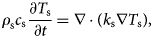
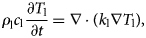
with Eqn (1) for the solid (x s) and Eqn (2) for the liquid (x l). Here, T is temperature, t is time, ρ is density, c is specific heat capacity and k is thermal conductivity. The thermal diffusivity is α = k/ρc. The third governing equation is for molecular diffusion in the solution which is defined by the same fundamental equation as above (i.e. Fickian diffusion)
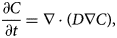
where C is the concentration of solute (in kg m−3) and D is the molecular diffusivity.
The three governing equations above are coupled at the phase boundary. The coupling is described mathematically by the Stefan condition, which dictates wall motion based on the heat flux in both solid and liquid media
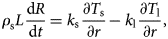
where L is the latent heat of fusion, R is the phase boundary location (i.e. the borehole radius for cylindrical coordinates) and r is the radial coordinate. Heat flows down the temperature gradient, so a negative gradient in the solid (temperature decreasing away from the hole) causes freezing. The act of freezing gives off thermal energy to the ice at the hole wall which will eventually diffuse out into the bulk ice. During active drilling, there is an imposed heat flux (Q) at the phase boundary, so an additional term can be included in Eqn (4). A secondary Stefan condition is added for the molecular diffusion problem

This condition states that the solute flux at the hole wall is dependent on the rate at which the wall moves. Conceptually, Eqn (5) expresses either solute rejection and accumulation in the case of borehole freezing (∂R/∂t is negative) or solute dilution in the case of borehole melting (∂R/∂t is positive). Thus, even when no additional mass of solute is added to the solution, freezing of the hole wall acts as a source term for the solute concentration and melting of the hole wall as a sink term.
To close the model, one additional equation is necessary which describes the concentration-dependent freezing temperature and fixes the thermal boundary condition at the hole wall for both Eqns (1) and (2),
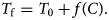
Here, T 0 is the pure liquid freezing temperature and f(C) is a function for freezing-point depression. We assign the freezing-point depression empirically (Supplementary Material S.1).
All model results below are reported in non-dimensional units: r* = r/R 0, R* = R/R 0 where R 0 is the drilled radius (0.04 m in our case), T* = T/T ∞ where T ∞ is the bulk ice temperature (−20 °C in our case), t* = t/t 0 where $t_0 = R_0^2 L/k_{\rm s}\vert {T_\infty } \vert$ . The model domain is 1-dimensional (radial), and the imposed heat flux for melting out the initial hole is constant (Q = 2.5 kW). Adjusting the problem-specific parameters (i.e. R 0, T ∞, and Q) would change the precise timing and magnitude of borehole evolution, but the qualitative conclusions presented below are consistent for any choice of parameters. For cases in which the numerical model can be tested analytically, those tests were done (Supplementary Material S.2).
3 Sequence of borehole stabilization
We use the equations described above to simulate borehole melting/freezing in the presence of an antifreeze solution for an ensemble of injection timings and volumes. Unlike prior studies, we emphasize the hot-point case where downward drilling motion is relatively slow but antifreeze can be injected soon after the drill passes through the borehole. For every simulation, the antifreeze solution is aqueous methanol and is considered ‘well mixed’ immediately after injection. Hence, the solution concentration and temperature are constant throughout the borehole while the solution dissolves the hole wall, reducing the model to Eqns (1) and (4). During this instantaneous-mixing phase, our model matches Humphrey and Echelmeyer (Reference Humphrey and Echelmeyer1990) exactly, including the numerics of the logarithmic transform and non-dimensionalization (Jarvis and Clarke, Reference Jarvis and Clarke1974; Humphrey and Echelmeyer, Reference Humphrey and Echelmeyer1990). The concentration within the hole is updated purely based on volume changes of the hole, and the solution temperature is assumed to match the depressed freezing temperature. The mixing process is exothermic, so thermal energy is added to the solution immediately after antifreeze injection.
We divide the simulation into four stages based on the dominating process for each stage. An example hole radius through time and a representative temperature profile from each stage are shown in Figure 1:
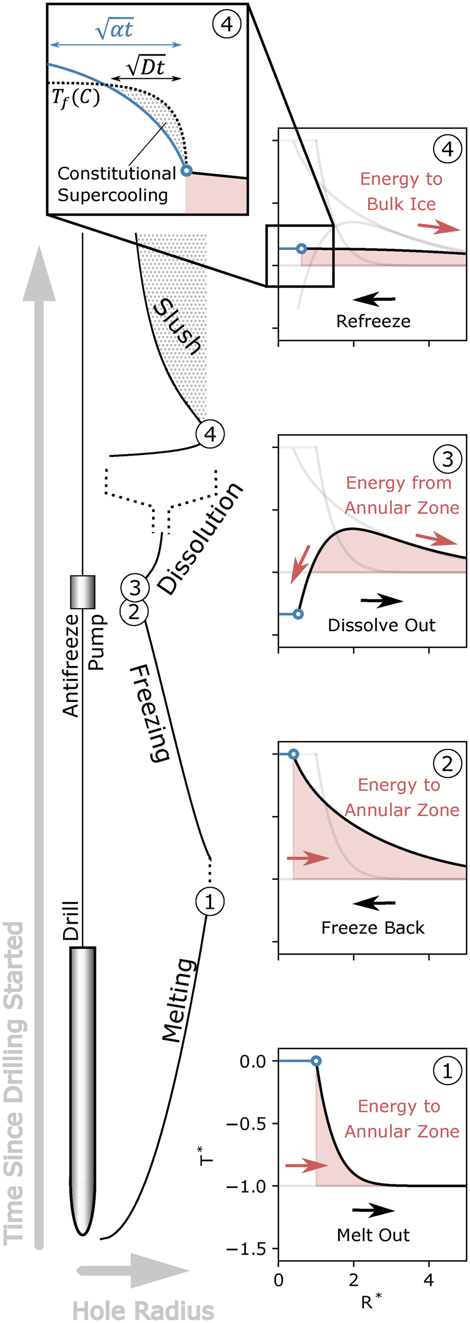
Fig. 1. A time series of borehole melting and refreezing. The labeled black line shows the hole radius through time from when drilling starts (bottom) to where the borehole stabilizes with slush forming in the solution (top). The horizontal scale changes at stage 4 to emphasize peak dissolution and subsequent slush formation (indicated by the expanding dashed lines). Representative temperature profiles are shown for each stage (1–4) with black the temperature in the ice, gray the temperature in a previous stage, blue the temperature in the solution which changes with the solution concentration, and the red area showing the warm thermal annulus in the ice. The inset for stage 4 is a cartoon representation which shows the competition between thermal and molecular diffusion that causes constitutional supercooling (slush) where the solution is colder than the liquidus line.
Stage 1. Melting – The melting stage is defined by a heat flux that follows the borehole wall as it moves outward. In addition to the energy for melting ice and moving the borehole wall outward, there is inevitably some amount of energy that goes toward warming ice in an annular zone outside the hole wall. The amount of warming in this thermal annulus is dependent on the rate of drilling with the fastest drilling being the most efficient to direct its energy toward melting while only minimally warming the ice (in the Supplementary Material S.3, we assess the influence of drilling speed on the two-dimensionality of an advection-diffusion problem for the down going drill).
Stage 2. Freezing – After the drill melts out the hole and the heat flux at the hole wall is removed, the energy in the hole begins to diffuse outward into the bulk ice; that is, the hole begins to freeze shut. During this process, the warm thermal annulus continues to grow as the latent energy within the hole is converted to thermal energy in the encroaching ice. The rate of freezing is rapid at first when the temperature gradient at the hole wall is greatest. Then, freezing slows down as the temperature gradient flattens out but the hole is still a substantial fraction of its original volume. Finally, when the hole approaches closure, the rate of freezing accelerates again because the total hole volume to freeze decreases non-linearly with the decreasing radius (i.e. volume is dependent on the square of the radius).
Stage 3. Dissolution – Antifreeze can be injected into the borehole to stop Stage 2 before the hole freezes shut. In all simulations, the injected antifreeze is at 0 °C, but directly after injection, the solution mixes and cools to the freezing temperature of the newly mixed solution. For some time, the solution is colder than the surrounding ice within the thermal annulus. Therefore, energy from the annulus initially moves back toward the hole center and causes the hole wall to re-melt (or dissolve). The total amount of dissolution depends on the size of the thermal annulus, as well as the total amount and rate of antifreeze injection. We assume that the dissolution process happens quickly after injection (all simulations shown here are on the scale of ~hours) and the hole therefore remains well mixed. If, on the other hand, the effect of molecular diffusion is considered important, the antifreeze solution would be diluted near the hole wall as ice dissolves, and the rate-limiting factor for dissolution would be the molecular diffusion of antifreeze toward the hole wall which is orders of magnitude slower than thermal diffusion for most solutions.
Stage 4. Refreezing (Slush) – Eventually, the dissolution in Stage 3 dissipates all the energy from the thermal annulus. If, at this stage, the solution temperature is colder than the bulk-ice temperature, the hole wall continues to dissolve and refreezing as slush is avoided entirely. If, on the other hand, the thermal annulus was large enough to dissolve the hole and warm the solution above the bulk-ice temperature, the energy that was originally directed toward dissolution moves back into the bulk ice and the hole refreezes. In the case of a well-mixed hole, refreezing happens as in Stage 2, by accretion on the hole wall. However, the timescale for this process (~days) is significantly longer than Stage 3 and unless there is some forced mixing within the hole, a solute gradient will be established. In this case, solute accumulates within a short distance (~millimeters) of the hole wall, with the exact characteristic length scale determined by the molecular diffusivity ($\sqrt {Dt}$ ). As solute accumulates, the solution temperature is depressed to the freezing temperature at the hole wall. Then, thermal and molecular diffusion compete within the hole. Thermal diffusion acts to distribute the latent energy of freezing throughout the solution, while molecular diffusion acts to distribute the accumulated solute that is rejected from the freezing ice lattice. For all cases in which the non-dimensional Lewis number (i.e. thermal over molecular diffusivity, Le = α/D) is greater than 1, the solution cools more quickly than solute moves. Then, slush forms in an area of ‘constitutional supercooling’ where the solution temperature is effectively below the freezing temperature (Fig. 1 stage 4 inset) (Worster, Reference Worster, Batchelor, Moffat and Worster2000). Considering aqueous methanol as the antifreeze agent Le ≫ 1, so we assume that all refreezing is in the form of slush.
To calculate the amount of dissolved and refrozen ice in our simulation results, we first assume that the borehole radius eventually converges to equilibrium, R eq. This radius is dependent on the total mass of injected antifreeze, M, and the bulk-ice temperature, T ∞,
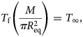
where $C_{{\rm eq}} = M/\pi R_{{\rm eq}}^2$ is the solution concentration at equilibrium volume, $V_{{\rm eq}} = \pi R_{{\rm eq}}^2$
 (per unit depth). Hence, the borehole changes size until the concentration is such that the depressed freezing temperature equals the bulk-ice temperature. The fraction of dissolved ice (Fig. 2a) is the ratio between the maximum dissolved borehole volume (V ④; Figure 1 stage 4) and the volume at injection (V ②; Figure 1 stage 2). It gives a measure of the over-dissolution of the hole before settling to the equilibrium volume. The fraction of refrozen ice (Fig. 2b) is the ratio between the equilibrium volume (V eq) and the maximum dissolved borehole volume (V ④). It gives an indication of the amount of slush formed. In some cases, enough antifreeze is injected that V ④ $ = V_{{\rm eq}}$
 and the refreezing stage is avoided altogether (white space in Fig. 2b).
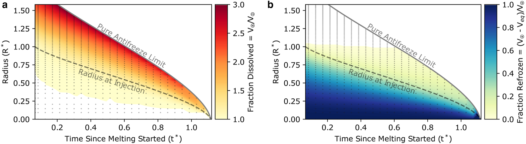
Fig. 2. Fraction dissolved (a) and fraction refrozen (b) results for an ensemble of simulations with variable injection timing and total mass of injected antifreeze. Each of the dots represents the result from one simulation, with its location on the plot being the timing of antifreeze injection and the equilibrium radius (proportional to the total mass of injected antifreeze through Eqn (7)). Fractional volumes shown by the colormaps are calculated after the entire simulation runs as described in the text, and colors are interpolated between individual simulations (i.e. individual dots). The radius at injection (dashed line) provides a reference for the state of the hole before any dissolution or refreezing. The pure antifreeze limit (solid line) is the equilibrium radius when the solution is pure antifreeze at the time of injection.
4. Discussion and conclusions
The cylindrical Stefan model that we use here, originally developed and tested for hot-water drilling methods (Humphrey and Echelmeyer, Reference Humphrey and Echelmeyer1990), reveals possible strategies for minimizing or even entirely avoiding slush formation by targeting a sufficiently large equilibrium radius. In Figure 2, we show that the fraction of the borehole to be refrozen as slush is substantially reduced when the equilibrium radius is greater than that at the time of injection. Moreover, when the equilibrium radius is larger than the melted radius there is no refrozen slush at all because the hole dissolves until the solution temperature equals the bulk-ice temperature and the system is in equilibrium. For hot-water holes, these cases are impractical because the antifreeze cannot be added until the entire hole has been drilled (unless drilling with an antifreeze solution as was one suggestion from Humphrey and Echelmeyer (Reference Humphrey and Echelmeyer1990)). Perhaps more interestingly, refreezing is also substantially decreased with later injection timing. When the hole is allowed to refreeze for some time before injection, some of the energy moves far enough into the bulk ice that the dissolution process does not recapture it, and therefore, the refrozen fraction is smaller.
Aside from timing the injection and providing sufficient antifreeze, one alternative strategy to avoid dissolution and subsequent refreezing is to slow down the rate of antifreeze injection (Humphrey and Echelmeyer, Reference Humphrey and Echelmeyer1990 Fig. 13) (Supplementary Material S.4). When the antifreeze concentration within the borehole slowly increases over time, the thermal annulus around the borehole has time to dissipate into the bulk ice rather than being directed toward dissolving the hole wall. The engineering design for this type of slow injection is somewhat natural for the hot-point drill because the pump is installed behind the drill to inject antifreeze throughout the drilling process. Assuming continuous injection and some vertical mixing, the solution at a given depth sees the moving pump as a sort of Gaussian source. While this approach of delayed injection always reduces the fraction of refrozen ice, perfect timing is impossible for any practical drilling scenario. This should be used as a mitigation technique, as opposed to an assumption of slush elimination, and paired with the cautionary overestimate of required antifreeze.
Refreezing is inevitable for some cases. This is especially true when the desired equilibrium radius is unattainable because the corresponding amount of antifreeze is logistically impractical. In these cases, convection (i.e. solution mixing) within the hole could prevent slush formation. Assuming sufficient mixing, the hole will freeze as accretion at the hole wall instead of slush in the solution. There are several natural sources of convection within the hole such as air bubbles moving upward in the hole as well as thermal convection. These violate the assumption of Fickian diffusion in Eqns (1), (2), and (3) but only act to help mitigate slush formation. In the hot-point drilling case, there are also some convenient options for forced convection, such as to continuously pump solution into the hole, to add some sort of flexible ‘whiskers’ onto the drill cable which will mix the solution as the drill descends, or to move a mass up and down the drilling cable. Each of these comes with its own setbacks and limitations; for example, any time that more features or instruments are added to the hole it increases the likelihood that something will freeze to the borehole wall, obstructing the rest of the drilling process.
The direct utility of the results presented here in terms of engineering design is significantly complicated by the fact that the bulk ice temperature is never known precisely. In areas with simple ice flow and a melted bed, the uncertainty in ice temperature is perhaps small, on the order of a few degrees. Where the bed is frozen, uncertainty in the geothermal flux estimate (e.g. Shapiro and Ritzwoller, Reference Shapiro and Ritzwoller2004) will lead to slightly higher temperature uncertainty. The greatest uncertainty in ice temperature comes in areas with strong heat generation such as an ice-stream shear margin (Jacobson and Raymond, Reference Jacobson and Raymond1998). At any location, we suggest that a sufficiently cautionary design would either include solution mixing during and after the drilling process, or enough antifreeze to stabilize the borehole at a colder temperature than expected. Any surplus antifreeze will only dissolve the hole past its melted radius.
Supplementary material
The supplementary material for this article can be found at https://doi.org/10.1017/aog.2020.70. Model code is available at https://github.com/benhills/CylindricalStefan.
Acknowledgements
We thank three anonymous reviewers for their input which greatly improved the original manuscript. We thank Justin Burnett for many valuable conversations which enabled and enhanced this work. This work was funded by the National Science Foundation Office of Polar Programs grant 1744787 and the National Aeronautics and Space Administration grant NNX17AF68G.


 Open access