the Creative Commons Attribution 4.0 License.
the Creative Commons Attribution 4.0 License.
 | 12 Oct 2020
Assessing soil salinity dynamics using time-lapse electromagnetic conductivity imaging
Maria Catarina Paz
Mohammad Farzamian
Ana Marta Paz
Nádia Luísa Castanheira
Maria Conceição Gonçalves
Fernando Monteiro Santos
Lezíria Grande de Vila Franca de Xira, located in Portugal, is an important agricultural system where soil faces the risk of salinization due to climate change, as the level and salinity of groundwater are likely to increase as a result of the rise of the sea water level and consequently of the estuary. These changes can also affect the salinity of the irrigation water which is collected upstream of the estuary. Soil salinity can be assessed over large areas by the following rationale: (1) use of electromagnetic induction (EMI) to measure the soil apparent electrical conductivity (ECa, mS m−1); (2) inversion of ECa to obtain electromagnetic conductivity imaging (EMCI) which provides the spatial distribution of the soil electrical conductivity (σ, mS m−1); (3) calibration process consisting of a regression between σ and the electrical conductivity of the saturated soil paste extract (ECe, dS m−1), used as a proxy for soil salinity; and (4) conversion of EMCI into salinity cross sections using the obtained calibration equation.
In this study, EMI surveys and soil sampling were carried out between May 2017 and October 2018 at four locations with different salinity levels across the study area of Lezíria de Vila Franca. A previously developed regional calibration was used for predicting ECe from EMCI. Using time-lapse EMCI data, this study aims (1) to evaluate the ability of the regional calibration to predict soil salinity and (2) to perform a preliminary qualitative analysis of soil salinity dynamics in the study area. The validation analysis showed that ECe was predicted with a root mean square error (RMSE) of 3.14 dS m−1 in a range of 52.35 dS m−1, slightly overestimated (−1.23 dS m−1), with a strong Lin's concordance correlation coefficient (CCC) of 0.94 and high linearity between measured and predicted data (R2=0.88). It was also observed that the prediction ability of the regional calibration is more influenced by spatial variability of data than temporal variability of data. Soil salinity cross sections were generated for each date and location of data collection, revealing qualitative salinity fluctuations related to the input of salts and water either through irrigation, precipitation, or level and salinity of groundwater. Time-lapse EMCI is developing into a valid methodology for evaluating the risk of soil salinization, so it can further support the evaluation and adoption of proper agricultural management strategies, especially in irrigated areas, where continuous monitoring of soil salinity dynamics is required.
- Article
(3926 KB) - Full-text XML
- BibTeX
- EndNote


Lezíria Grande de Vila Franca de Xira (hereafter called Lezíria de Vila Franca) is an important agricultural system of alluvial origin located by the estuary of the Tejo River, north-east of Lisbon, Portugal (Fig. 1), where soil faces risk of salinization due to the marine origin of part of the sediments, tidal influence of the estuary, irrigation practices, and projected evolution of future climate with increasing temperature and decreasing precipitation. Traditional soil salinity investigations have been conducted in the study area using the electrical conductivity of a saturated soil paste extract (ECe, dS m−1) as a proxy for soil salinity. However, they were limited to a few boreholes and involved soil sampling, which restricted the analysis to point information, often lacking representativeness at the field scale. In addition, borehole drilling is invasive and not feasible to conduct over large areas, given the large number of boreholes that needs to be made.
Electromagnetic induction (EMI) is widely used as a non-invasive and cost-effective solution to map soil properties over large areas. EMI measures the apparent electrical conductivity of the soil (ECa, mS m−1), which is a function of soil properties such as salinity, texture, cation exchange capacity, water content, and temperature. However, in a saline soil, soil salinity is generally the dominant factor responsible for the spatiotemporal variability of soil ECa when soil is moist. EMI surveys have been successfully used in conjunction with soil sampling to assess soil salinity through location-specific calibration between measured ECa and soil salinity (e.g. Triantafilis et al., 2000, 2001; Corwin and Lesch, 2005; Bouksila et al., 2012; Corwin and Scudiero, 2019; Kaufmann et al., 2019; von Hebel et al., 2019). However, the ability of this method to map soil salinity distribution with depth is limited. This is because EMI measures ECa, a depth-weighted average conductivity measurement, which does not represent the soil electrical conductivity (σ, mS m−1) with depth. More recently, a state-of-the-art approach called electromagnetic conductivity imaging (EMCI) has permitted the generation of σ from the inversion of multi-height and/or multi-sensor ECa data (Monteiro Santos, 2004; Dafflon et al., 2013; von Hebel et al., 2014; Farzamian et al., 2015; Shanahan et al., 2015; Jadoon et al., 2015; Moghadas et al., 2017). When comparing σ with the soil properties sampled in boreholes, such as ECe, soil water content, and pH, a calibration process is developed through a regression between σ and the soil properties. Thus, EMCI can be converted to a cross section of the soil properties which show strong correlation with σ. This methodology has been applied in Lezíria de Vila Franca to study soil salinity risk (Farzamian et al., 2019; Paz et al., 2019b) and salinity and sodicity risk (Paz et al., 2019a). In this later study, the authors performed a principal component analysis of the soil properties in the study area and found that the water content was correlated with σ but with a relatively lower influence when compared to the properties related to salinity and sodicity (ECe, sodium adsorption ratio, and exchangeable sodium percentage).
Because the inversion of ECa is relatively recent since the use of EMI for soil characterization, the lack of validation using an independent dataset still limits the use of this new methodology (Corwin and Scudiero, 2019), making it therefore important to further test its accuracy in salinity monitoring.
When repeated over a period of time at the same place, EMCI becomes time-lapse EMCI and can be used to investigate the dynamics of soil properties such as soil water content (Huang et al., 2017, 2018; Moghadas et al., 2017). Using time-lapse EMCI data, this study aims (1) to evaluate the ability of a previously developed regional calibration to predict soil salinity and (2) to perform a preliminary qualitative analysis of soil salinity dynamics in the study area. For this purpose, EMI measurements and soil sampling were carried out between May 2017 and October 2018 at four locations with different salinity levels across the study area. EMI measurements were performed with a single-coil instrument (EM38), collecting ECa data in the horizontal and vertical orientations and at two heights, and then inverted to obtain EMCI, which provides a vertical distribution of σ. Finally, σ was converted to ECe using the previously developed regional calibration. Soil samples were collected along the EMI transects and used for laboratory determination of ECe. These data were used as an independent dataset to evaluate the ability of the regional calibration to predict soil salinity and to generate soil salinity cross sections for each date of data collection.
2.1 Study area
The study was carried out in Lezíria de Vila Franca, a peninsula of alluvial origin surrounded by the Tejo and Sorraia rivers, and the Tejo estuary, located 10 km north-east of Lisbon, Portugal, as shown in Fig. 1. Soils in this region have fine to very fine texture and are classified as Fluvisols in the northern part and as Solonchaks in the southern part, according to the Harmonized World Soil Database (Fischer et al., 2012). Climate is temperate with hot and dry summers, according to the Köppen classification. Daily measurements of precipitation, mean temperature, and reference evapotranspiration recorded during the study period at the meteorological station represented by the blue circle in Fig. 1b are shown in Fig. 2. Land use in this area (of about 130 km2) is constituted by irrigated annual crops in the northern part and mainly by rainfed pastures in the southern part. Irrigation is ensured by an infrastructure that covers most of the area, collecting surface water at the confluence of the two rivers. The irrigation water has low salinity with electrical conductivity typically below 0.5 dS m−1 and a sodium adsorption ratio below 1 (mmolc L−1)0.5. The area exhibits a north–south soil salinity gradient which influences the distribution of land-use types and which is probably due to the regional distribution of the marine fraction of sediments and to the saline influence of the estuary on groundwater in the southern part.
Four locations were chosen in the study area, as presented in Fig. 1b, with numbers 1 to 4. Locations 1, 2, and 3 are cultivated with annual rotations of irrigated herbaceous crops in spring and annual ryegrass (Lolium multiflorum) in the autumn, with ploughing usually once a year. During the study years (2017 and 2018), the spring crop at location 1 was tomato drip irrigated, and at locations 2 and 3 it was maize irrigated by centre pivots. Location 4 is a rainfed spontaneous pasture that has not been ploughed at least in the last 10 years. During the study period, location 1 was irrigated from 12 April to 23 July 2017 and from 30 May to 23 September 2018; location 2 was irrigated from 17 June to 11 October 2017 and from 24 May to 22 September 2018; and location 3 was irrigated from 17 May to 10 September 2017 and from 6 June to 17 September 2018. Groundwater level is shallow, as expected in an estuarine environment, and has saline characteristics. In the southern part of the study area, closer to the estuary, the depth and salinity of groundwater are influenced by tidal variation.
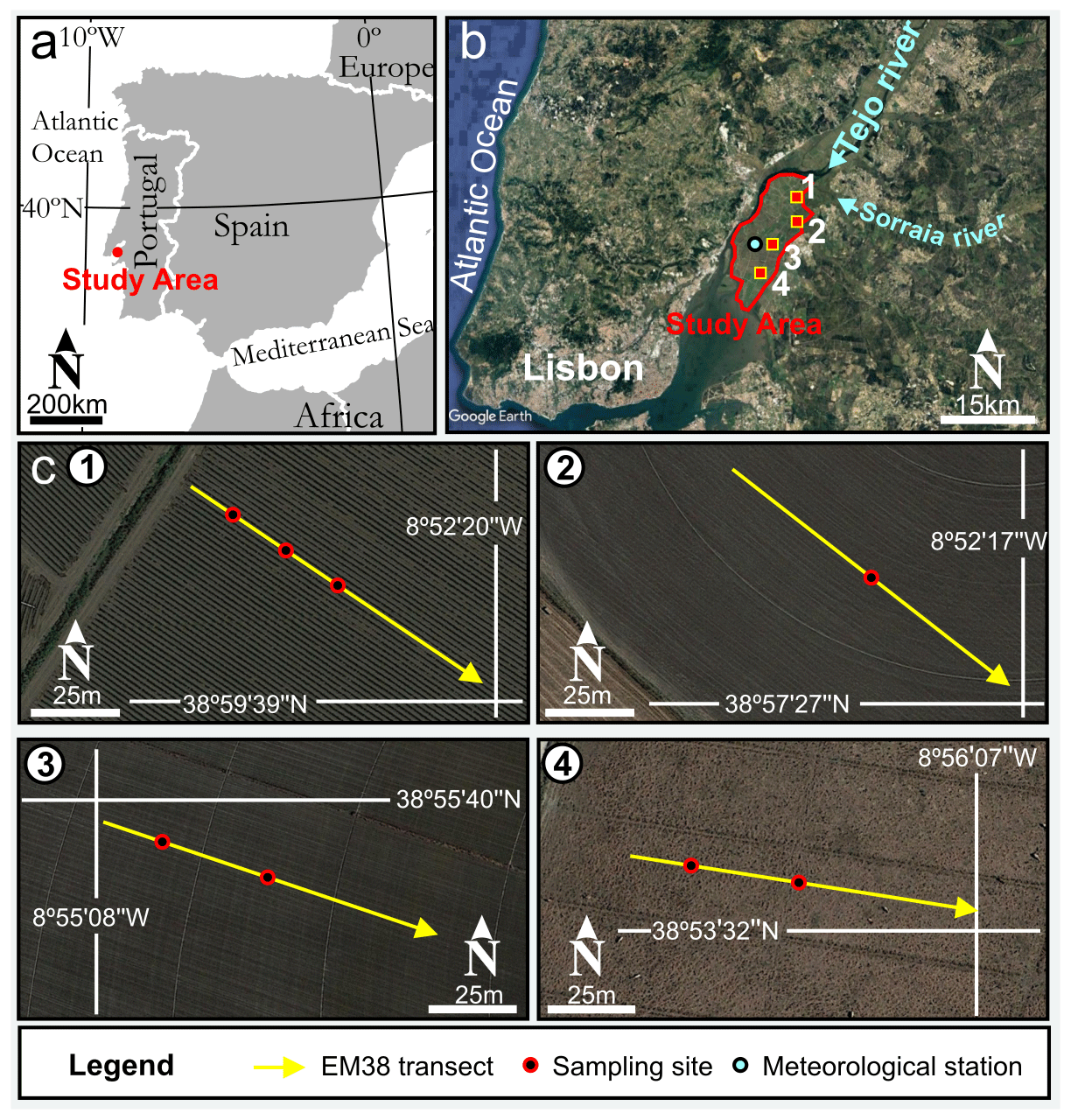
Figure 1(a–b) Location of the study area in Portugal, showing the main geographical features and the four locations; (c) details of the four locations showing the EM38 transects and the soil sampling sites © Google Earth.
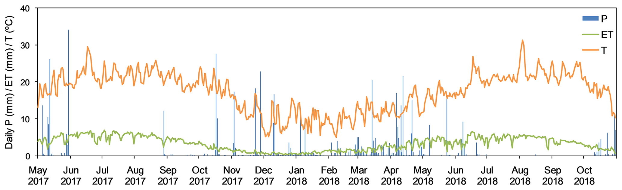
Figure 2Distribution of daily precipitation (P), reference evapotranspiration (ET), and mean temperature (T) recorded at the meteorological station located in the study area during the study period.
2.2 Electromagnetic induction data acquisition and inversion
EMI data were acquired using the EM38 instrument (Geonics Ltd, Mississauga, Canada). Technology of this instrument is based on two coils, one transmitting the electromagnetic signal and the other receiving it, distanced 1 m apart from each other inside the instrument case. The position of these coils can be controlled by placing the instrument in a vertical position relative to the soil surface – horizontal dipole mode (the coils stand in the horizontal position), which provides a maximum depth of investigation of 1.5 m – or in a horizontal position relative to the soil surface – vertical dipole mode (the coils stand in the vertical position), which provides a maximum depth of investigation of 0.75 m. EM38 surveys were done on five dates at locations 1 and 4 and on six dates at locations 2 and 3, during the period of May 2017 to October 2018. Measurements on the first two dates were continuously acquired at each location, along a 100 m transect, using a GPS (Rikaline 6010, with 5 m position accuracy) for registration of the position. Subsequent EMI measurements were acquired at each location, along a 20 m transect. The middle point of each 20 m transect was coincident with the medium point of each previous 100 m transect. Measurements were acquired at positions 1 m apart along the 20 m transects (Fig. 1c), overlapping the medium section of the 100 m transects. ECa was collected at two heights from the soil surface (0.15 and 0.4 m) in the horizontal and vertical dipole orientations, which was ensured by placing the EM38 on a cart built specifically for this purpose. The cart has two shelves to accommodate the instrument, one at 0.15 m from the soil surface and the other at 0.40 m from the soil surface. Inversion of ECa data to obtain σ was carried out using a 1-D laterally constrained inversion algorithm (Monteiro Santos et al., 2011). The ECa responses of the model were calculated through forward modelling based on the full solution of the Maxwell equations (Kaufman and Keller, 1983). The subsurface model used in the inversion process consisted of a set of 1-D models distributed according to the position of the ECa measurements. The subsurface model at each measurement position was constrained by the neighbouring models, allowing the use of the algorithm in regions characterized by high conductivity contrast. An Occam regularization (De Groot-Hedlin and Constable, 1990) based approach was used to invert the ECa data. All ECa data, collected at the four locations, were inverted by applying a five-layer earth initial model with electrical conductivity of 100 mS m−1 and a fixed layer thickness of 0.30 m. To run the algorithm, several parameters were selected, such as the type of inversion algorithm, the number of iterations, and the smoothing factor (λ) that controls the roughness of the model. The optimal inversion parameters for the present conditions were obtained in previous studies for the study area (Farzamian et al., 2019).
Table 1Description and equations of the statistical indicators used to evaluate the prediction ability of the regional calibration in this work.
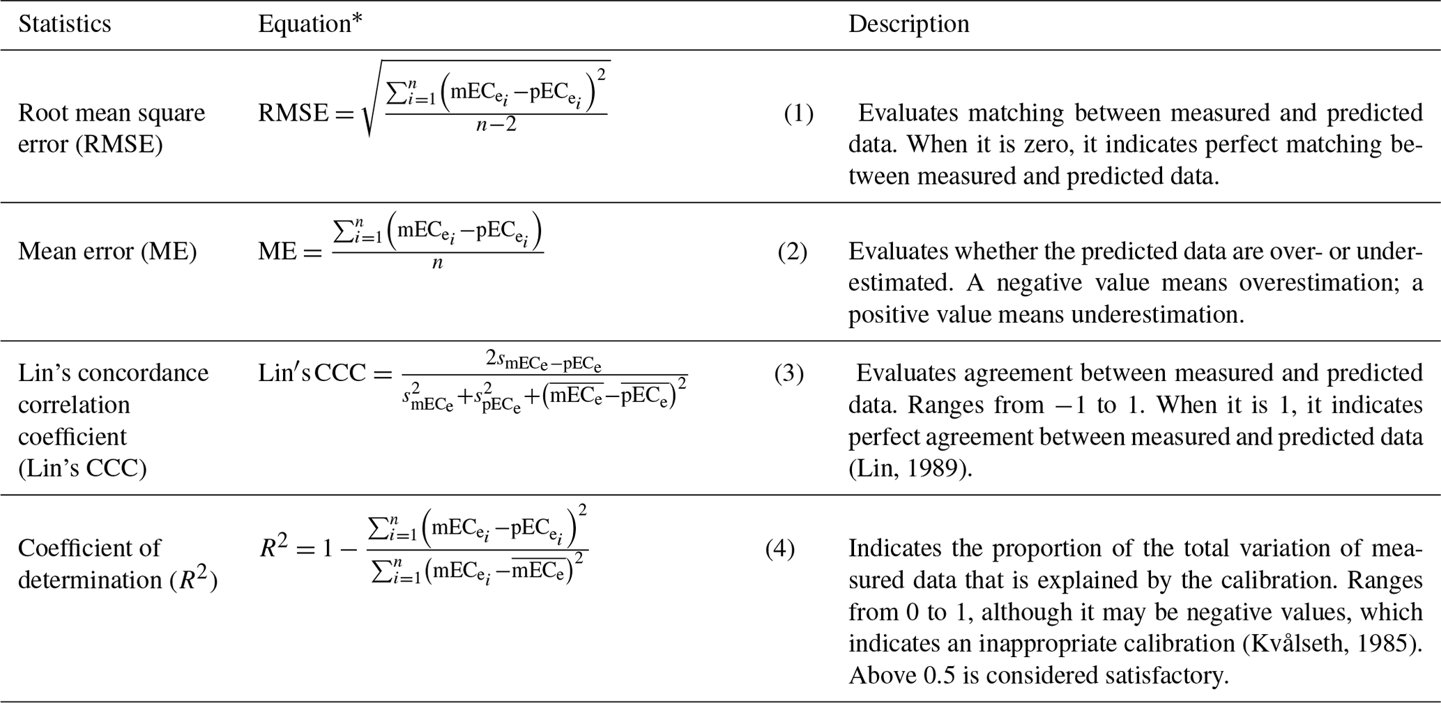
* n is the total number of data; mECe is measured ECe; pECe is predicted ECe; the upper bar represents the mean of the indicated data; s2 is the variance of the indicated data.
2.3 Soil sampling and laboratory analysis
Soil samples were collected at the same time as EMI surveys along the transects, as shown in Fig. 1c. At each sampling site, five soil samples were collected at 0.3 m increments, from a depth of 0.15 to 1.35 m, as a representation of topsoil (0–0.3 m), subsurface (0.3–0.6 m), upper subsoil (0.6–0.9 m), intermediate subsoil (0.9–1.2 m), and lower subsoil (1.2–1.5 m), to monitor water content and ECe. In the laboratory, water content was obtained using the gravimetric method and then converted to volumetric water content (θ – m3 m−3) after bulk density (g m−3) determination from undisturbed 100 cm3 soil samples. ECe was measured with a conductivity meter (WTW 1C20-0211 inoLab) in the extract collected from the soil saturation paste obtained from 300 g of air-dry soil samples, according to the methods described by Richards (1954). In this study, the soil is classified according to its ECe level as non-saline (ECe<2 dS m−1), slightly saline (2–4 dS m−1), moderately saline (4–8 dS m−1), highly saline (8–16 dS m−1), and severely saline (>16 dS m−1), according to the terminology proposed by Barrett-Lennard et al. (2008).
2.4 Prediction of ECe from time-lapse EMCI
A regional calibration to predict ECe from σ was previously developed for the study area, resulting in the linear equation ECe=0.03σ–1.05 (Farzamian et al., 2019). This calibration was termed “regional” because the equation was obtained using all ECe and σ data collected at four locations in the study area. Farzamian et al. (2019) tested the regional and location-specific calibrations, verifying that they have comparable prediction ability. However, the regional calibration can be used at any new location in the study area, within the range of measured ECe, which makes it highly suitable for mapping salinity in the study area. The regional calibration was based on data collected during May and June 2017 and was validated using a leave-one-out cross-validation method with good results (RMSE = 2.54 dS m−1 in the 0–37 dS m−1 range). The detailed calibration and cross-validation procedures are described in Farzamian et al. (2019).
In the present study, the regional calibration was used to predict ECe from time-lapse EMCI (pECe). The predicted ECe and ECe measured from soil samples (mECe), collected at the same time as the EMI surveys, were used as an independent dataset for the validation of the regional calibration. The validation was performed by calculating the root mean square error (RMSE), the coefficient of determination (R2) between the measured and predicted ECe, Lin's concordance correlation coefficient (CCC), and the mean error (ME). Description of these statistical indicators and the equations used to calculate them are shown in Table 1. Calculations were done using global data and also using data discriminated by date of measurement (in this case we considered dates when measurements were done at the four locations – January, June, and October 2018).
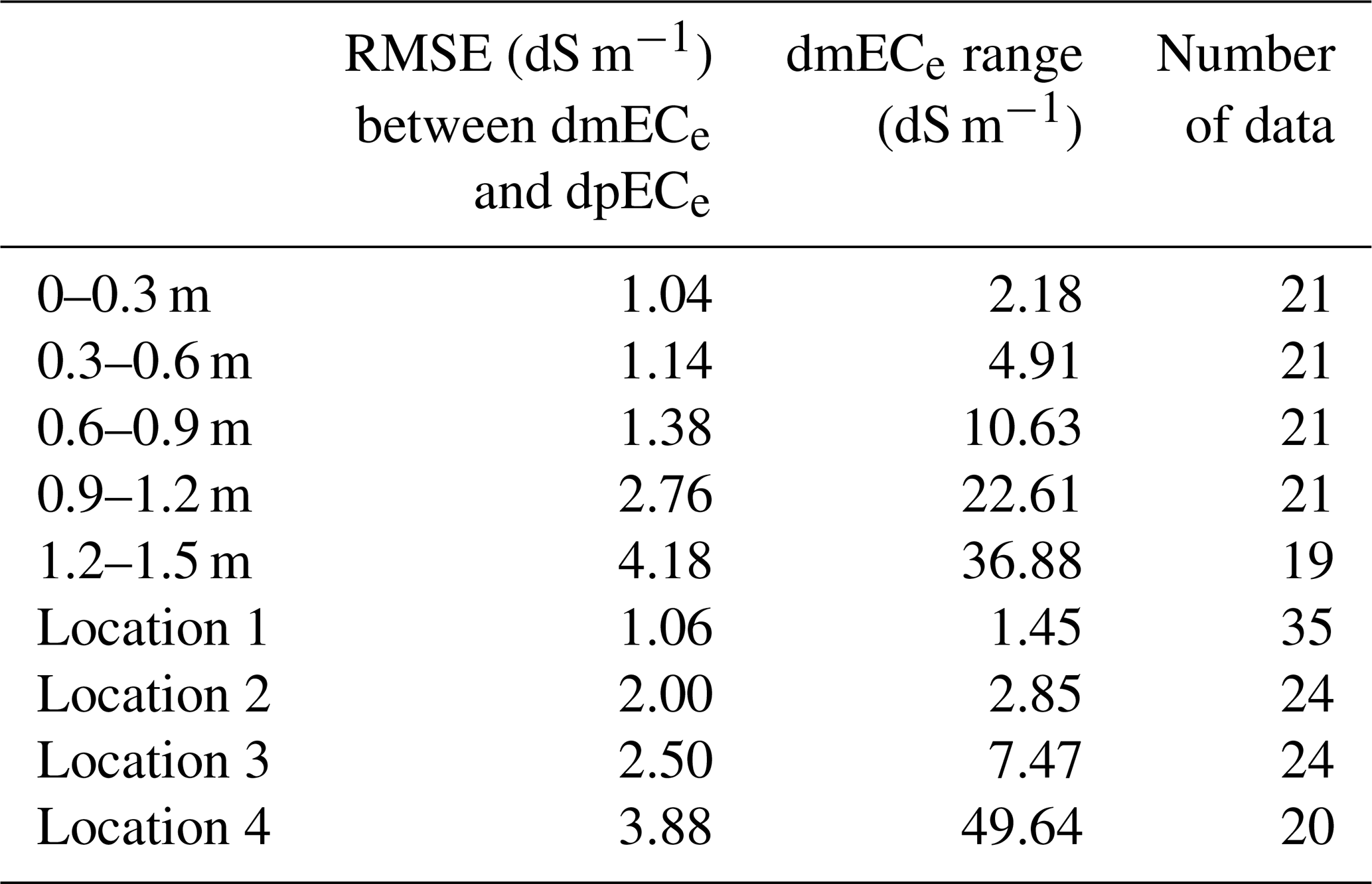
To further explore the spatial and temporal sensitivity of the regional calibration and to investigate whether the regional calibration can be used to assess soil salinity variability at different locations and depths, we calculated the RMSE between the deviations of mECe (dmECe) and the deviations of pECe (dpECe) for each soil depth and location. These deviations were calculated by using the following equations:
in which the means were calculated with the values referent to each date of measurement for each soil depth and location. RMSE was then calculated between dmECe and dpECe according to Eq. (1).
3.1 Temporal variation of measured θ and ECe
Figure 3 shows the variation of θ and ECe with time at the sampling site located in the middle of each transect (Fig. 1c), at locations 1 to 4. At location 1, θ increases with depth and the lower subsoil (1.2–1.5 m) is permanently saturated within the study period. In the more superficial layers until 0.9 m depth, the influence of rainfall, evapotranspiration, and irrigation is noticeable. For instance, in the topsoil, θ peaks in January 2018 and lowers during the dry seasons, because drip irrigation during the dry seasons has a localized effect and there is high water uptake by the crop. At location 2, unlike the other locations, the lower subsoil is unsaturated. The influence of rainfall, evapotranspiration, and irrigation is also noticeable. At locations 3 and 4, θ also increases with depth and the intermediate and lower subsoil layers are permanently saturated.
Regarding ECe, at location 1 the values observed are always below 1 dS m−1, except for the topsoil in September and October 2018, which is probably due to fertigation practices during the irrigation period. At location 2, ECe generally increases with depth. All layers show a peak in June and July 2018, probably due to fertigation practices. At location 3, ECe reaches higher levels than at the previous locations, exceeding 4 dS m−1, which is the generally accepted threshold for the classification of saline soils. Location 4 presents the highest ECe of all locations. At the topsoil the values are below 4 dS m−1 but increase consistently with depth to about 50 dS m−1 in the lower subsoil. The increase in ECe during June 2018 can be due to the influence of saline groundwater.
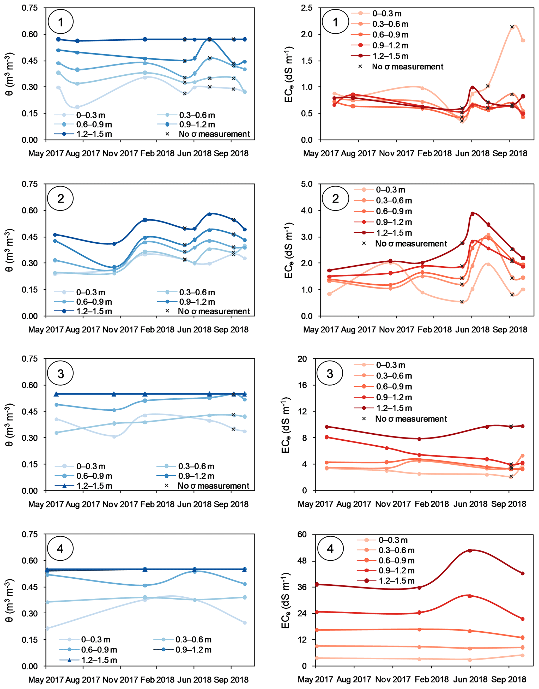
Figure 3Volumetric water content (θ – m3 m−3) and electrical conductivity of the soil saturation extract (ECe – dS m−1) in the topsoil (0–0.3 m), subsurface (0.3–0.6 m), upper subsoil (0.6–0.9 m), intermediate subsoil (0.9–1.2 m), and lower subsoil (1.2–1.5 m), measured in the sampling site located at the middle of each transect, at locations 1 to 4, during the study period. Each circled number refers to each location. Crosses refer to the dates when there were ECe measurements but no σ measurements, due to adverse field conditions.
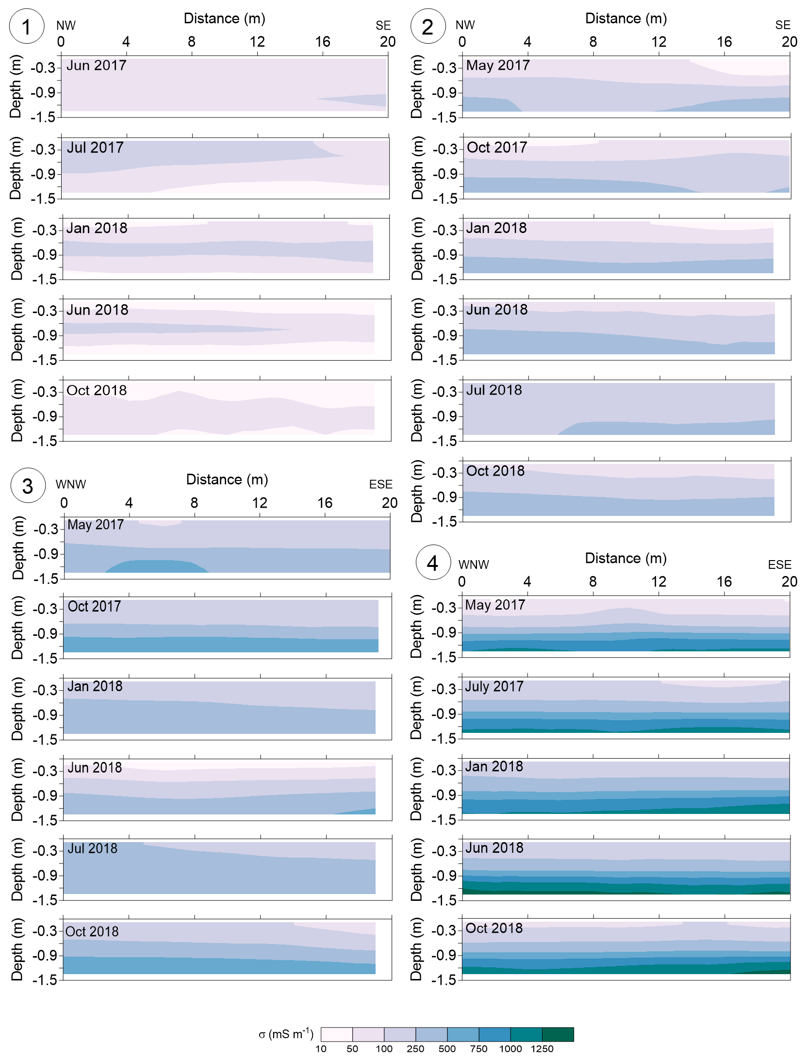
3.2 Time-lapse EMCIs
Figure 4 shows the obtained EMCIs at locations 1 to 4 for each date of the EMI surveys. Globally, σ ranges from 19.44 to 1431.57 mS m−1, with the lowest values at location 1 and the highest at location 4. A general increasing trend of σ is quite evident from the north to the south, accompanying the previously known soil salinity gradient. In addition, σ increases with depth at locations 2, 3, and 4. At location 1, σ ranges spatiotemporally from 19.44 to 128.08 mS m−1. At location 2, σ ranges from 28.02 to 469.39 mS m−1, with the highest values at depth. A similar pattern of σ is evident at locations 3 and 4. However, a greater range of σ is seen at location 3, with values from 36.23 to 706.32 mS m−1. Location 4 exhibits the largest variations of σ, ranging from 48.57 to 1431.57 mS m−1.
3.3 Prediction of ECe using the regional calibration
Figure 5 shows ECe predicted with the regional calibration versus the measured ECe and the 1:1 line, with points identified in terms of date of measurement (Fig. 5a) and depth of measurement (Fig. 5b). Table 2 shows the statistical indicators obtained using global data, i.e. data collected at all locations, from July 2017 to October 2018, and the statistical indicators for each date. The validation of the regional calibration using global data resulted in a RMSE of 3.14 dS m−1 and a R2 of 0.88, which indicates satisfactory prediction ability, given the large range of ECe (52.35 dS m−1). High global Lin's CCC of 0.94 shows agreement between measured and predicted ECe. The ME is −1.23 dS m−1, indicating that the regional calibration generally overestimates ECe. Figure 5a and b show that the points are generally scattered around the 1:1 line, and it is not possible to identify variations depending on the date or depth of the measurement. In order to analyse the prediction ability at each location, Fig. 5c and d display an enlargement of the lower left parts of the previous figures, displaying ECe values below 15 dS m−1. Figure 5c and d show differences in the prediction ability according to the location, namely at locations 2 and 3, where ECe is generally overestimated. At location 2, ECe is more overestimated in deeper soil layers (Fig. 5d), which is likely due to the clay content that consistently increases with depth at this location, while it is rather uniform or declines with depth at the other locations (Farzamian et al., 2019). At location 3, ECe is also overestimated, most likely due to the influence of θ and cation exchange capacity (Paz et al., 2019a), which are higher on average compared to locations 2 and 4. Finally, the ECe ranges of location 4 and of the lower subsoil are similar to the ECe range of global data, showing dominance of location 4 and of lower subsoil data on the calibration. On the other hand, the statistical indicators discriminated by date of measurement (in this case we considered only the dates when measurements were done at the four locations – January, June, and October 2018), shown in Table 2, reveal that the prediction ability does not vary significantly when comparing the statistical indicators of the three dates. These results suggest that spatial variability of data has a much stronger influence on the prediction ability of the regional calibration than temporal variability of data.
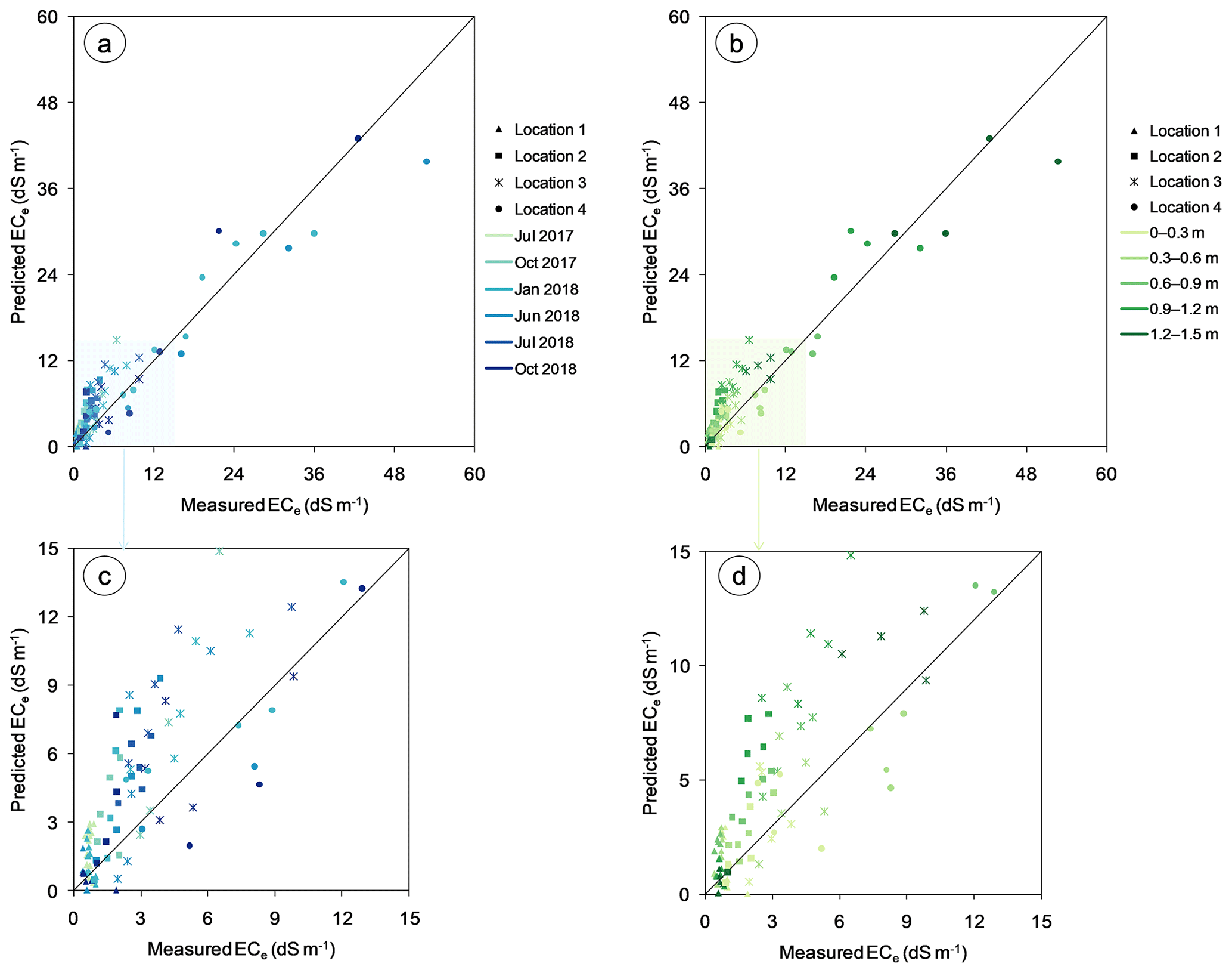
Figure 5Plots of predicted ECe versus measured ECe and the 1:1 line, obtained for locations 1 to 4, identified in terms of date of measurement (a) and depth of measurement (b). Plots (c) and (d) show enlargements of the lower left parts of plots (a) and (b), respectively.
Table 2RMSE, ME, Lin's CCC, R2, minimum, maximum, and range of ECe, and the number of data used to calculate these statistical indicators, discriminated in terms of global and date of measurement.
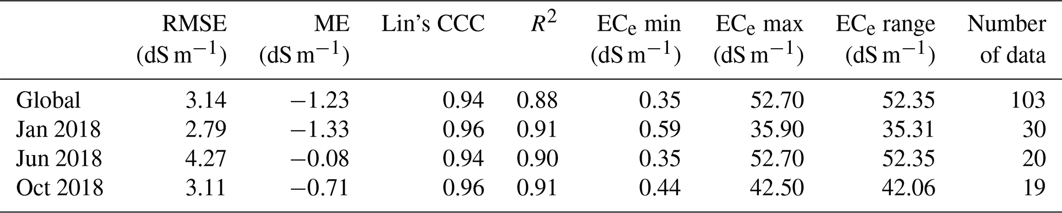
Table 3 shows the RMSE between dmECe and dpECe obtained for each soil depth and each location. The RMSE is 1.04 dS m−1 at the topsoil, which is relatively high given the small range of deviation variability (2.18 dS m−1). This indicates that it is difficult to estimate soil salinity variability at topsoil from time-lapse EMI data and regional calibration. We attribute the weak prediction ability at topsoil to the small range of ECe variability and to the larger variability of other soil properties (e.g. θ and temperature) at topsoil, which are due to different irrigation schemes and cultivated crops at each location. The results of RMSE show better prediction ability at the subsurface and very good prediction ability at upper, intermediate, and lower subsoil, suggesting that the time-lapse EMI data and regional calibration can be used to assess soil salinity changes in these soil layers. On the other hand, the RMSE results for each location show that the prediction ability is poor for monitoring of soil salinity variability at location 1 (1.06 dS m−1) and location 2 (2.00 dS m−1) given the small range of deviation variability at these locations. This is not surprising as the soil is non-saline at location 1, with a very small range of ECe (0.35–1.89 dS m−1), and slightly saline at location 2, with a small range of ECe (0.91–3.86 dS m−1). Thus, other soil properties such as θ and clay content have a larger impact on the spatiotemporal variability of σ. In addition, larger variations of ECe and σ at location 4 dominated the regional regression calibration, further limiting the application of the regional calibration for monitoring the small variability of soil salinity at locations 1 and 2. The RMSE results are better to some extent at location 3 and very good at location 4, suggesting that the time-lapse EMI data and regional calibration can fairly predict soil salinity variability at location 3 and very well at location 4.
This spatial sensitivity of the regional calibration can be improved by studying new locations across the study area to include a wider variability of soil properties and ranges of ECe in the regression calibration. On the other hand, longer observation periods and more frequent EMI surveying and soil sampling, as well as monitoring of other soil dynamic properties that influence σ (i.e. θ, soil temperature, level and salinity of groundwater), and finding ways to quantitatively account for their impact on time-lapse EMCIs, can improve the temporal sensitivity of regional calibrations.
Table 3RMSE between dmECe and dpECe, range of dmECe, and the number of data used to calculate RMSE, discriminated in terms of depth of measurement and location.
3.4 Generation of soil salinity cross sections from time-lapse EMCI
Figure 6 shows the soil salinity cross sections (ECe predicted using the regional calibration) at locations 1 to 4 for each date of the EMI surveys, categorized into six salinity classes, ranging from non-saline to severely saline. The measured ECe and the groundwater level at the sampling site located in the middle of each EMI transect are also shown.

Figure 6Cross sections of soil salinity (predicted ECe) for locations 1 to 4, with representation of measured ECe (in circles) and groundwater level (blue triangles) at the sampling sites located in the middle of each transect. Note that in June 2018 at location 3 and in July 2017 at location 4 there was no soil sampling.
The salinity cross sections for location 1 show that the soil is generally non-saline, with slightly saline zones on all dates except for October 2018. These saline zones occur in the top soil layers until 0.9 m depth (topsoil, subsurface and upper subsoil) and represent an overestimation of the soil salinity when compared to the measured ECe of the sampling point (which is invariably non-saline). This overestimation tendency is in agreement with Fig. 5d, where the very low range of spatiotemporal variations of soil salinity at this location can also be observed. In such conditions, other soil properties, such as θ, dominate the small variations of σ, and therefore the ability to predict salinity from σ at this location was reduced as discussed in Sect. 4.3. Our previous studies with both location-specific and regional calibrations tested at this location showed similar results (Farzamian et al., 2019).
At location 2 the salinity cross sections show an increase in salinity with depth from non-saline at the topsoil to highly saline in the lower subsoil, with the exception of July 2018, where the entire soil profile is moderately saline. The increase in soil salinity in the upper soil layers in July 2018 can be attributed to fertigation practices for the maize cultivation that introduced salts into the soil profile. The salinity cross sections also show the overestimation of salinity occurring mainly in the deeper soil layers, which agrees with the results presented in Fig. 5d and discussed in Sect. 4.3.
At location 3 soil salinity is well predicted in May 2017 but tends to be slightly overestimated on the remaining dates, especially in July 2018. The salinity cross sections show that salinity increases with depth, reaching severely saline in May 2017 and October 2017. This can be due to the influence of the saline groundwater (as seen in Fig. 3, the intermediate and lower subsoil layers are permanently saturated). The groundwater level is above 1.5 m in January 2018, although the salinity of the deeper soil layers (>0.9 m) decreases compared to May and October 2017, which could be due to washing of the profile by rainfall. The increase in soil salinity in the upper soil layers in July 2018, similarly to location 2 on the same date, can be attributed to fertigation practices for the maize cultivation.
At location 4 the trend of increasing salinity with depth is accurate on all dates, but it tends to be slightly underestimated. The salinity cross sections show that salinity increases from non-saline in topsoil to severely saline in lower subsoil. This is probably related to the saline groundwater level above 1.5 m. During the dry period of the year, salinity of the lower subsoil reaches the highest values (June 2018).
Comparison of the salinity cross sections between locations confirms the previously known north–south soil salinity spatial gradient of the study area; that is, from location 1 to location 4, soil salinity generally increases. Soil salinity dynamics at each location reveals fluctuations in time related to the input of salts and water either through irrigation, precipitation, or groundwater level and salinity. Location 1 tends to have non-saline characteristics, which can be attributed to good-quality irrigation. In addition, this location is far from the estuary, making it less prone to the presence of saline groundwater. At locations 2 and 3, the salinity cross sections show an increase in soil salinity in the upper layers during the dry season (when irrigation occurs), which decreases in the following months with increased rainfall (Fig. 2). At location 4, an increment of salinity along the entire profile is visible during the dry season. This is likely due to the influence of the saline groundwater and capillary rise along the profile.
In this study, EMI and soil sampling data collected between May 2017 and October 2018 were used, together with a previously developed regional calibration, to predict soil salinity. This procedure allowed further validation of the regional calibration with an independent dataset and a preliminary qualitative analysis of soil salinity dynamics in the study area. Based on the comprehensive analysis of the statistical indicators obtained from the validation process and the obtained soil salinity cross sections, the following main conclusions can be drawn.
The validation performed in this study resulted in a RMSE of 3.14 dS m−1, which is acceptable given the large range of ECe (52.35 dS m−1). This validation resulted in lower prediction ability than that previously resulting from cross-validation (which had a RMSE of 2.54 dS m−1). This is expected because the test set is completely independent of the dataset used to develop the calibration and was collected over a wider period of time (18 months). During this period, soil properties, which are also known to influence σ, such as temperature and θ, change, which introduces larger variability in data.
The prediction ability of the regional calibration does not vary significantly over time. As a result, the regional calibration approach still stands as an expeditious method to predict soil salinity from EMI surveys at any new location in the study area. However, prediction ability of the regional calibration in assessing variability of soil salinity at different depths and locations varies significantly due to variability of soil properties at each depth and location. Our investigation shows that significantly larger variations of ECe and σ at location 4 dominated the regional regression calibration, suggesting a good prediction ability of the regional calibration in the south of the study area and close to location 4, where the soil salinization is of major concern and can compromise agricultural activity.
The methodology used in this study allowed the generation of soil salinity cross sections displaying the patterns of soil salinity at different dates, at four locations in the study area. The salinity cross sections show a qualitative response of soil salinity to the input of salts and water either through irrigation, precipitation, or level and salinity of groundwater. In a regional perspective, soil salinity dynamics in the study area may be preliminarily explained by a combination of spatial distribution of the marine fraction of soil, with irrigation practices in the study area and saline groundwater in the southern part.
Application of time-lapse EMCI and calibration for assessing soil salinity dynamics is a developing methodology that can further support the evaluation and adoption of proper agricultural management strategies in irrigated regions. Some aspects can and will be addressed in future studies so as to improve its performance. From this study, we identify some of these aspects. First, relative to the inversion process and in the absence of a time-lapse inversion algorithm, ECa data were inverted independently. This method can distort the inversion results, since the reference model and a priori information are not considered. Further research involves time-lapse inversion algorithms that are being developed to invert data collected with EMI sensors, which can generate EMCIs of higher precision. Secondly, the influence of static soil properties (i.e. that do not vary in time), such as clay content and cation exchange capacity, could be tackled with the use of cross sections of the variation of soil salinity between two consecutive dates, which allows removal of the static effect from the time-lapse EMCIs. Finally, temporal soil salinity assessment can be optimized by quantitatively taking into account the influence of soil dynamic properties on the time-lapse EMCIs. Specifically, in Lezíria, regional calibrations can be improved by studying new locations across the study area for a longer period of time with more frequent surveying and sampling and also by including new parameters, such as θ, soil temperature, level, and salinity of groundwater. However, the temporal variations of these properties are connected to location-specific conditions. For instance, θ can vary significantly in the study area, particularly in the root zone, due to different irrigation practices, root uptake of different crops, and fluctuation of groundwater level. These facts highlight the necessity of using location-specific calibrations for a more precise assessment of soil salinity changes at each location.
The data were acquired at privately owned farms and are not available to the public.
MCP and MF designed the EMI surveys, processed and inverted time-lapse EMI data, performed the statistical analysis, and generated the main results. AMP, NLC, and MCG collected soil samples, performed the laboratory analysis, and contributed to the statistical analysis. FMS developed the code for inversion of EMI data. MCP, MF, AMP, and NLC wrote the text. MCP prepared the visualization. MCG and FMS contributed to the elaboration of the methodology and discussion of the results.
The authors declare that they have no conflict of interest.
The authors are grateful to the Associação de Beneficiários da Lezíria Grande de Vila Franca de Xira and to Manuel Fernandes and Fernando Pires from INIAV for the field assistance. This research was performed within projects of“Salinization in irrigated areas: risk evaluation and prevention” (SALTFREE) and “Sustainable use of soil and water for improving crops productivity in irrigated areas” (SOIL4EVER). Mohammad Farzamian was supported by a contract within project SOIL4EVER. This publication is supported by FCT – project UIDB/GEO/50019/2019 – Instituto Dom Luiz. We are very grateful for the helpful and constructive comments of the editor Jan Vanderborght and two anonymous reviewers, who helped to significantly improve the paper.
This research has been supported by the Fundação para a Ciência e a Tecnologia (grant nos. ARIMNET2/0004/2015, ARIMNET2/0005/2015, and PTDC/ASP-SOL/28796/2017).
This paper was edited by Jan Vanderborght and reviewed by two anonymous referees.
Barrett-Lennard, E. G., Bennett, S. J., and Colmer, T. D.: Standardising the terminology for describing the level of salinity in soils. In: Proceedings of the 2nd international salinity forum: Salinity, water and society global issues, local action, Adelaide, SA, Australia, 31 Mar.–3 Apr. 2008. Geological Society of Australia, Hornsby, NSW, Australia, 2008.
Bouksila, F., Persson, M., Bahri, A., and Berndtsson, R.: Electromagnetic inductionprediction of soil salinity and groundwater properties in a Tunisian Saharan oasis, Hydrol. Sci. J., 57, 1473–1486, https://doi.org/10.1080/02626667.2012.717701, 2012.
Corwin, D. L. and Lesch, S. M.: Characterizing soil spatial variability with apparent soilelectrical conductivity: I. Survey protocols, Comp. Elec. Agri. Appl. Apparent Soil Elec. Conductivity Precis. Agri., 46, 103–133, https://doi.org/10.1016/j.compag.2004.11.002, 2005.
Corwin, D. L. and Scudiero, E.: Chapter One - Review of soil salinity assessment for agriculture across multiple scales using proximal and/or remote sensors, Adv. Agron., 158, 1–130, https://doi.org/10.1016/bs.agron.2019.07.001, 2019.
Dafflon, B., Hubbard, S., Ulrich, C., and Peterson, J. E.: Electrical conductivity imaging of active layer and permafrost in an arctic ecosystem, through advanced inversion of electromagnetic induction data, Vadose Zone J., 12, 1–19, https://doi.org/10.2136/vzj2012.0161, 2013.
De Groot-Hedlin, C. and Constable, S. C.: Occam's inversion to generate smooth, two-dimensional models from magnetotelluric data, Geophysics, 55, 1613–1624, https://doi.org/10.1190/1.1442813, 1990.
Farzamian, M., Monteiro Santos, F. A., and Khalil, A. M.: Application of EM38 and ERT methods in estimation of saturated hydraulic conductivity in unsaturated soil, J. Appl. Geophys., 112, 175–189, https://doi.org/10.1016/j.jappgeo.2014.11.016, 2015.
Farzamian, M., Paz, M. C., Paz, A. M., Castanheira, N. L., Gonçalves, M. C., Santos, F. A. M., and Triantafilis, J.: Mapping soil salinity using electromagnetic conductivity imaging-a comparison of regional and location-specific calibrations, Land Degrad. Dev., 30, 1393–1406, https://doi.org/10.1002/ldr.3317, 2019.
Fischer, G., Nachtergaele, F. O., Prieler, S., Teixeira, E., Toth, G., van Velthuizen, H., Verelst, L., and Wiberg, D.: Global Agro-ecological Zones (GAEZ v3.0)-Model Documentation [WWW Document], available at: http://www.fao.org/soils-portal/soil-survey/soil-maps-and-databases/harmonized-world-soil-database-v12/en/ (last access: 17 December 2018), 2012.
Huang, J., Purushothaman, R., McBratney, A., and Bramley, H.: Soil water extraction monitored per plot across a field experiment using repeated electromagnetic induction surveys, Soil Syst., 2, 11, https://doi.org/10.3390/soilsystems2010011, 2018.
Huang, J., Scudiero, E., Clary, W., Corwin, D. L., and Triantafilis, J.: Time-lapse monitoring of soil water content using electromagnetic conductivity imaging, Soil Use Manage., 33, 191–204, https://doi.org/10.1111/sum.12261, 2017.
Jadoon, K. Z., Moghadas, D., Jadoon, A., Missimer, T. M., Al-Mashharawi, S. K., and McCabe, M. F.: Estimation of soil salinity in a drip irrigation system by using joint inversion of multicoil electromagnetic induction measurements, Water Resour. Res., 51, 3490–3504, https://doi.org/10.1002/2014WR016245, 2015.
Kaufman, A. A. and Keller, G. V.: Frequency and transient soundings. Methods in Geochemistry and Geophysics, 16. Elsevier, New York, https://doi.org/10.1111/j.1365-246X.1984.tb02230.x, 1983.
Kaufmann, M. S., von Hebel, C., Weihermüller, L., Baumecker, M., Döring, T., Schweitzer, K., Hobley, E., Bauke, S. L., Amelung, W., Vereecken, H., et al., and van der Kruk, J.: Effect of fertilizers and irrigation on multi-configuration electromagnetic induction measurements, Soil Use Manage., 36, 104–116, https://doi.org/10.1111/sum.12530, 2019.
Kvålseth, T. O.: Cautionary note about R2, Am. Stat., 39, 279–285, https://doi.org/10.1080/00031305.1985.10479448, 1985.
Lin, L. I. K.: A concordance correlation coefficient to evaluate reproducibility. Biometrics, 45, 255–268, https://doi.org/10.2136/sssaj1998.03615995006200010030x, 1989.
Moghadas, D., Jadoon, K. Z., and McCabe, M. F.: Spatiotemporal monitoring of soil water content profiles in an irrigated field using probabilistic inversion of time-lapse EMI data, Adv. Water Resour., 110, 238–248, https://doi.org/10.1016/j.advwatres.2017.10.019, 2017.
Monteiro Santos, F. A.: 1-D laterally constrained inversion of EM34 profiling data, J. Appl. Geophys., 56, 123–134, https://doi.org/10.1016/j.jappgeo.2004.04.005, 2004.
Monteiro Santos, F. A., Triantafilis, J., and Bruzgulis, K.: A spatially constrained 1D inversion algorithm for quasi-3D conductivity imaging: application to DUALEM-421 data collected in a riverine plain, Geophysics, 76, B43–B53, https://doi.org/10.1190/1.3537834, 2011.
Paz, A., Castanheira, N., Farzamian, M., Paz, M. C., Gonçalves, M., Monteiro Santos, F., and Triantafilis, J.: Prediction of soil salinity and sodicity using electromagnetic conductivity imaging, Geoderma, 361, https://doi.org/10.1016/j.geoderma.2019.114086, 2019a.
Paz, M. C., Farzamian, M., Monteiro Santos, F., Gonçalves, M. C., Paz, A. M., Castanheira, N. L., and Triantafilis, J.: Potential to map soil salinity using inversion modelling of EM38 sensor data, First Break, 37, 35–39, https://doi.org/10.3997/1365-2397.2019019, 2019b.
Richards, L. A. (Ed.): Diagnosis and Improvement of Saline and Alkali Soils. Agricultural Handbook, USDA, Washington, D.C., USA, 1954.
Shanahan, P. W., Binley, A., Whalley, W. R., and Watts, C. W.: The use of electromagnetic induction to monitor changes in soil moisture profiles beneath different wheat genotypes, Soil Sci. Soc. Am. J., 79, 459–466, https://doi.org/10.2136/sssaj2014.09.0360, 2015.
Triantafilis, J., Laslett, G. M., and McBratney, A. B.: Calibrating an electromagnetic induction instrument to measure salinity in soil under irrigated cotton, Soil Sci. Soc. Am. J., 64, 1008–1017, https://doi.org/10.2136/sssaj2000.6431009x, 2000.
Triantafilis, J., Odeh, I. O. A. V., and McBratney, A. B.: Five geostatistical methods to predict soil salinity from electromagnetic induction data across irrigated cotton, Soil Sci. Soc. Am. J., 65, 869–978, https://doi.org/10.2136/sssaj2001.653869x, 2001.
von Hebel, C., van der Kruk, J., Huisman, J. A., Mester, A., Altdorff, D., Endres, A. L., Zimmermann, E., Garré, S., and Vereecken, H.: Calibration, Conversion, and Quantitative Multi-Layer Inversion of Multi-Coil Rigid-Boom Electromagnetic Induction, Sensors, 19, 4753, https://doi.org/10.3390/s19214753, 2019.
von Hebel, C., Rudolph, S., Mester, A., Huisman, J. A., Kumbhar, P., Vereecken, H., and van der Kruk, J.: Three-dimensional imaging of subsurface structural patterns using quantitative large-scale multi-configuration electromagnetic induction data, Water Resour. Res., 50, 2732–2748, https://doi.org/10.1002/2013wr014864, 2014.