On the Calculation of Propulsive Characteristics of a Bulk-Carrier Moving in Head Seas

Abstract

The present work describes a simplified Computational Fluid Dynamics (CFD) approach in order to calculate the propulsive performance of a ship moving at steady forward speed in head seas. The proposed method combines experimental data concerning the added resistance at model scale with full scale Reynolds Averages Navier–Stokes (RANS) computations, using an in-house solver. In order to simulate the propeller performance, the actuator disk concept is employed. The propeller thrust is calculated in the time domain, assuming that the total resistance of the ship is the sum of the still water resistance and the added component derived by the towing tank data. The unsteady RANS equations are solved until self-propulsion is achieved at a given time step. Then, the computed values of both the flow rate through the propeller and the thrust are stored and, after the end of the examined time period, they are processed for calculating the variation of Shaft Horsepower (SHP) and RPM of the ship’s engine. The method is applied for a bulk carrier which has been tested in model scale at the towing tank of the Laboratory for Ship and Marine Hydrodynamics (LSMH) of the National Technical University of Athens (NTUA).

1. Introduction

The problem of a self-propelled ship is one of the most challenging in Naval Architecture since the Engineer is facing an unsteady Three-dimensional (3D) flow, characterized by high Reynold’s number, significant viscous effects, the presence of free surface and the complex interaction between the hull and the propeller. Taking into account incident waves makes the problem even harder. Traditionally, the problem of the self-propelled ship in a seaway was tackled experimentally in model scale by separating the problem of the self-propelled ship in calm water from the problem of added resistance in waves. Thus, the solution could only be approximated. Even when a self-propelled scale model is used, the extrapolation of the results to the full-scale ship is problematic due to the scale effect on viscous resistance [1].

Computational Fluid Dynamics (CFD) methods solving the Reynolds Averaged Navier–Stokes (RANS) equations have become of age and are widely used to predict the resistance and propulsion characteristics of ships [2]. Time-dependent RANS solvers have also been developed and can yield promising results with regards to the 6-degrees-of-freedom (6DOF) motions of a ship as well as the added resistance in waves [3]. Solving the time-dependent self-propulsion problem of a ship in waves has proven to be quite time consuming, thus hybrid methods have been proposed. Such methods calculate the effect on the propulsive characteristics of the ship motions, via semi-empirical methods for the prediction of the effect on the ship wake [4].

In recent years, several methods have been proposed in order to solve the problem of the self-propelled ship in incident waves [3,5,6,7,8]. In most cases, only regular waves are considered due to the high computational cost of such methods. There are some publications that attempt to solve the complete problem of the self-propelled ship in irregular waves [9]. However, these methods require significant computing power in order to obtain accurate results. Therefore, some simplifications are required in order to achieve reliable results and to reduce the computational cost. In this respect, we present a hybrid method for predicting the propulsion characteristics of a ship in irregular head seas in this work, which combines experimental data with CFD calculations.

Having as a starting point experimental model-scale resistance and sea-keeping measurements, we numerically solve the full-scale propulsion problem, where the thrust requirements on the propeller are based on the extrapolation of the model-scale resistance measurements. In this extrapolation, the scale effects are taken into account. Also, the required thrust is obtained by solving the self-propulsion problem, i.e., by calculating the wake fraction and thrust deduction ratio. The actual flow problem is solved by employing the in-house developed RANS solver in conjunction with an actuator disk model for the propeller. The method is used to calculate the propulsion characteristics of a bulk carrier traveling at a steady forward speed in irregular head waves.

2. The Numerical Method

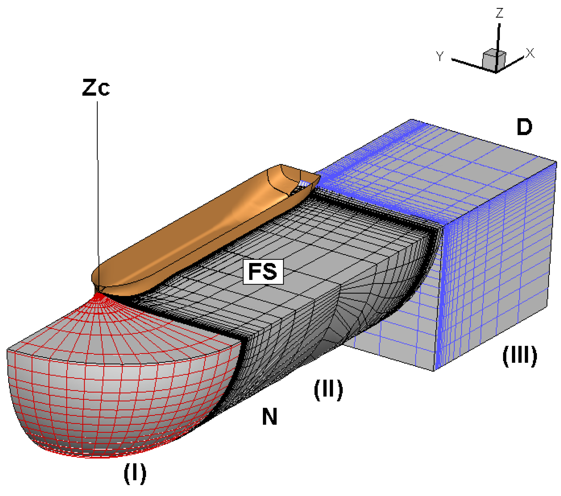
The employed method has been developed at the Laboratory for Ship and marine Hydrodynamics (LSMH) of the National Technical University of Athens (NTUA). It solves the RANS equations in a body fitted structured mesh as shown in Figure 1. The three regions (I), (II) and (III) refer to three different grid topologies. Region (I) consists of a C-O grid following a sequence of transverse planes which intersect on the Zc-axis. Region (II) represents an H-O grid which is formed by transverse planes to the longitudinal symmetry x-axis, while region (III) forms a typical H-H grid which is generated when a dry or wet transom stern exists, [2]. The C-O topology is applicable for bulbus bow configurations. The H-O grid is the standard grid in most CFD applications around ship hulls. Finally, the H-H is suggested for transom sterns exhibiting discontinuity when the transom is wetted [10].

In any case, the 2D grids on the transverse planes are generated following the conformal mapping technique as described in [10]. In order to apply as far as possible high grid resolutions, the three blocks are created in a restricted domain underneath the predetermined free surface boundary (FS). The free surface is calculated according to the hybrid potential viscous flow method [2].

The RANS code employs a sequence of orthogonal curvilinear systems bounded on each transverse plane. In such a system the three velocity components are denoted as (u_i, u_j, u_l) and the u_i- momentum equation reads:

$$\begin{array}{cc}\hfill C\left(u_i\right)=& -\frac{1}{h_i}\frac{\partial p}{\partial x_i}+\rho u_j^2{K}_{\mathit{ji}}+\rho u_l^2{K}_{\mathit{li}}-\rho u_i{u}_j{K}_{\mathit{ij}}-\rho u_i{u}_l{K}_{\mathit{il}}+\left({\sigma }_{\mathit{ii}}-{\sigma }_{\mathit{jj}}\right)K_{\mathit{ji}}\hfill \\ & +\left({\sigma }_{\mathit{ii}}-{\sigma }_{\mathit{ll}}\right)K_{\mathit{li}}+{\sigma }_{\mathit{ij}}\left({2K}_{\mathit{ij}}+K_{\mathit{lj}}\right)+{\sigma }_{\mathit{il}}\left({2K}_{\mathit{il}}+K_{\mathit{jl}}\right)+\frac{1}{h_i}\frac{\partial {\sigma }_{\mathit{ii}}}{\partial x_i}+\frac{1}{h_j}\frac{\partial {\sigma }_{\mathit{ij}}}{\partial x_j}+\frac{1}{h_l}\frac{\partial {\sigma }_{\mathit{il}}}{\partial x_l}\hfill \end{array}$$

(1)

where (h_i, h_j, h_l) are the metrics, K_ij = (1/h_ih_j)∂h_i/∂x_j the curvatures of the orthogonal system, ρ the fluid density, p the static plus the hydrostatic pressure, σ_ij the stress tensor and the left-hand side of Equation (1) represents the convective terms:

$$C\left(\Phi \right)=\rho \frac{\partial \Phi }{\partial t}+\frac{\rho }{h_i{h}_j{h}_l}\left[\frac{\partial \left(h_j{h}_l{u}_i\Phi \right)}{\partial x_i}+\frac{\partial \left(h_i{h}_l{u}_j\Phi \right)}{\partial x_j}+\frac{\partial \left(h_i{h}_j{u}_l\Phi \right)}{\partial x_l}\right]$$

(2)

The stress tensor components are associated to the deformation tensor through

$$\begin{array}{l}{\sigma }_{\mathit{ii}}=2{\mathsf{\mu }}_e{e}_{\mathit{ii}}=2{\mathsf{\mu }}_e\left[\frac{1}{h_i}\frac{\partial u_i}{\partial x_i}+u_j{K}_{\mathit{ij}}+u_l{K}_{\mathit{il}}\right]\\ {\sigma }_{\mathit{ij}}={\mathsf{\mu }}_e{e}_{\mathit{ij}}={\mathsf{\mu }}_e\left[\frac{h_j}{h_i}\frac{\partial }{\partial x_i}\left(\frac{u_j}{h_j}\right)+\frac{h_i}{h_j}\frac{\partial }{\partial x_j}\left(\frac{u_i}{h_i}\right)\right]\end{array}$$

(3)

The effective viscosity in Equation (3) is defined as

$${\mathsf{\mu }}_{\mathrm{e}}=\mathsf{\mu }+\rho {\mathsf{\nu }}_{\mathrm{t}}$$

(4)

where ν_t stands for the turbulent (or eddy) viscosity which is calculated according to the two-equation k-ω-SST turbulence model. The equation for the kinetic energy of turbulence k reads

$$\begin{array}{cc}\hfill C\left(k\right)=& \frac{1}{h_i{h}_j{h}_l}\left[\frac{\partial }{\partial x_i}\left({\sigma }_k{\mathsf{\mu }}_t\frac{h_j{h}_l}{h_i}\frac{\partial k}{\partial x_i}\right)+\frac{\partial }{\partial x_j}\left({\sigma }_k{\mathsf{\mu }}_t\frac{h_i{h}_l}{h_j}\frac{\partial k}{\partial x_j}\right)+\frac{\partial }{\partial x_l}\left({\sigma }_k{\mathsf{\mu }}_t\frac{h_i{h}_j}{h_l}\frac{\partial k}{\partial x_l}\right)\right]\hfill \\ & +G-{\mathsf{\beta }}^{*}\rho \omega k\hfill \end{array}$$

(5)

while the equation for the specific dissipation ω reads

$$\begin{array}{cc}\hfill C\left(\omega \right)=& \frac{1}{h_i{h}_j{h}_l}\left[\frac{\partial }{\partial x_i}\left({\sigma }_{\omega }{\mathsf{\mu }}_t\frac{h_j{h}_l}{h_i}\frac{\partial \omega }{\partial x_i}\right)+\frac{\partial }{\partial x_j}\left({\sigma }_{\omega }{\mathsf{\mu }}_t\frac{h_i{h}_l}{h_j}\frac{\partial \omega }{\partial x_j}\right)+\frac{\partial }{\partial x_l}\left({\sigma }_{\omega }{\mathsf{\mu }}_t\frac{h_i{h}_j}{h_l}\frac{\partial \omega }{\partial x_l}\right)\right]\hfill \\ & +\frac{\gamma }{v_t}G-{\mathsf{\beta }}^{*}\rho {\omega }^2+2\rho (1-F_1)\frac{{\sigma }_{\omega }}{\omega }\frac{1}{h_j^2}\frac{\partial k}{\partial x_j}\frac{\partial \omega }{\partial x_j}\hfill \end{array}$$

(6)

According to the k-ω-SST model, the turbulent kinematic viscosity is calculated according to the formula

$${\mathsf{\nu }}_t=\frac{a_{1}k}{max[a_1\mathsf{\omega },\left|rot(\overrightarrow{c})\right|F_2]}$$

(7)

In the above Equations (5)–(7), the constants σ_k, σ_ω, β* and the functions F₁, F₂ are defined as per the original paper of Menter [11], while G represents the generation term of the turbulence kinetic energy. Essentially, this model separates the flow-field above the body surface in two regions, which are determined according to the local flow parameters and the normal distance from the surface. The k-ω-SST model has been developed in order to calculate effectively complex flow fields, like those appearing in stern flows past full ship forms.

The momentum (RANS) and the turbulence model equations are solved numerically by applying the finite volume method in a staggered grid arrangement. In the resulting non-linear algebraic equations, the convective terms are approximated according to the second order MUSCL scheme [12] associated with the minmod limiter function [13], while the diffusive and the source terms are approximated using central differences. The solution follows the SIMPLE algorithm, where the RANS equations are solved following a marching scheme, while the pressure (continuity) equation is treated as fully elliptic.

Dirichlet boundary conditions are applied on the external boundary N of Figure 1 for the flow variables. The velocity components and the pressure on this boundary are calculated by the potential flow solution performed around the hull and the real free surface [14]. On the free surface, FS in Figure 1, the kinematic condition is fulfilled (zero normal velocity) while for the pressure and the turbulence quantities Neumann conditions are applied. In order to calculate the flow variables above the solid boundary in a uniform way, the standard wall function method is employed. On the exit plane D, open-type conditions hold [15]. Finally, on the flow symmetry plane, along the ship symmetry axis, the normal velocity component is set equal to zero while the normal derivatives of all other variables vanish (Neumann conditions). The exchange of the flow-variables on the matching planes between different blocks is based on a second order interpolation.

A number of domain sweeps is required to obtain convergence of the momentum and continuity equations. Convergence is achieved when the sum of the absolute residuals of the finite volume equations over all nodes becomes lower than a pre-specified criterion. In the present study, this criterion is set equal to 5 × 10⁻⁴ρV_S²A_M for the momentum equations and equal to 5 × 10⁻⁴ρV_SA_M for the continuity equation, where V_S represents the ship’s speed and A_M is equal to the transverse area covered by the grid at the mid-ship section.

The self-propulsion problem is solved by adopting the actuator disk model. To introduce this model, the effective wake is approximated according to the open water numerical experiment as in [16,17]. The propeller thrust is calculated following an iterative procedure so that its final value equals the total resistance of the ship. This procedure is also followed when the free surface problem is solved, since the stern wave is influenced by the propeller operation.

Regarding modeling the propulsion in waves, the fundamental simplification adopted in the described method, is that the ship moves in steady forward speed, under rough head sea conditions without performing any other motion, Under this assumption, the propeller thrust should be equal to the hydrodynamic resistance of the ship at any time, i.e.,

$${\mathrm{T}}_{\mathrm{P}}(\mathrm{t})={\mathrm{R}}_{\mathrm{T},\mathrm{S}}(\mathrm{t})$$

(8)

where T_P denotes thrust and R_T,S(t) the resistance. In addition, it is assumed that R_T,S(t) can be decomposed in two components as:

$${\mathrm{R}}_{\mathrm{T},\mathrm{S}}(\mathrm{t})={\mathrm{R}}_{\mathrm{C}\mathrm{W},\mathrm{S}}(\mathrm{t})+{\mathrm{R}}_{\mathrm{A}\mathrm{D},\mathrm{S}}(\mathrm{t})$$

(9)

In the above relation R_CW,S(t) represents the hydrodynamic resistance of the body moving in still water and R_AD,S(t) the added resistance due to the varying wave loads in sea route.

As an extension of the Froude hypothesis, R_AD,S(t) is considered as a wave resistance component depending only on the Froude number and is calculated as

$${\mathrm{R}}_{\mathrm{A}\mathrm{D},\mathrm{S}}(\mathrm{t})={\mathrm{C}}_{\mathrm{W},\mathrm{A}\mathrm{D}}(\mathrm{t})\times \frac{1}{2}\times \rho \times \mathrm{S}\times {\mathrm{U}}_{\mathrm{S}}{}^2$$

(10)

where C_W,AD(t) is the corresponding resistance coefficient, S is the wetted surface of the ship in still water and U_S the ships’ speed. Since C_W,AD(t) depends on the Froude number, it can be calculated by performing towing tank experiments at model scale. In these experiments, we can measure independently the total resistance of the model R_T,CW,M in calm water as well as the history of R_T,M(t) at a given sea state, always at steady forward speed.

Then, the coefficient C_W,AD(t) can be derived through

$${\mathrm{C}}_{\mathrm{W},\mathrm{A}\mathrm{D}}(\mathrm{t})=\frac{{\mathrm{R}}_{\mathrm{T},\mathrm{M}}(\mathrm{t})-{\mathrm{R}}_{\mathrm{T},\mathrm{C}\mathrm{W},\mathrm{M}}}{\frac{1}{2}\times \rho \times \mathrm{S}\times {\mathrm{U}}_{\mathrm{M}}{}^2}$$

(11)

Therefore, the added resistance in Equation (9) can be calculated at any time step, taking into account the scale difference in the time domain, i.e.,

$${\mathrm{t}}_{\mathrm{s}}=\sqrt{\mathsf{\lambda }}\times {\mathrm{t}}_{\mathrm{m}}$$

(12)

where t_s symbolizes the time in the ship scale, t_m the time in the model scale and λ is the geometrical scale ratio.

The reason that the component R_CW,S(t) in Equation (9) is a function of time, is that any change in the propeller thrust induces a different thrust deduction ratio and has to be calculated by performing an iterative procedure for each time step. In this procedure, the actuator disk model is based on the adoption of body forces that are exerted on fluid particles passing through the plane of the propeller blades. In the present approximation, only the axial body forces are taken into account, being included as source terms in the axial momentum equation. The radial distribution of the body forces is based on the lifting line method, as described in [18]. The body forces are integrated in the actual control volumes as described in [15,17].

The lifting line code requires two fundamental parameters, i.e., the propeller thrust and the velocities at infinite. Both of them are defined by performing a self-propulsion iterative procedure at each time step. In each internal iterative step, the propeller thrust T_P(t) is assumed to be equal to the body resistance of the previous step and changes the stern flow field accordingly. Then, a new total resistance R_CW,S(t), Equation (9), is calculated and the procedure stops when for three successive time steps self-propulsion is achieved, i.e., Equation (8) holds. Since the flow rate through the propeller blades changes as the iterations are performed, the required lifting line input data are changed accordingly. In addition, at a certain internal step an open water numerical experiment is performed as described by [16] in order to calculate the effective wake fraction at infinite as a function of the flow rate passing through the propeller disk.

The abovementioned procedure is straight forward and provides the history of T_P(t) almost independently of the exact distribution of body forces in each time step. Numerical experiments have shown that only an approximate prediction of the circulation distribution along the blades is required, which more or less remains similar under variable lifting line input conditions. However, when we need to calculate the required engine characteristics, we have to employ the lifting line output as concerned the required torque and rpm. To adapt these data, we assume that the propeller operates in a quasi-steady condition and therefore the steady lifting line approximation produces reasonable estimates for the required SHP and RPM.

In a further simplification of the problem, we can also consider the time averaged values for the resistance components of (9):

$$\overline{{\mathrm{R}}_{\mathrm{T}}}=\overline{{\mathrm{R}}_{\mathrm{C}\mathrm{W}}(\mathrm{t})}+\overline{{\mathrm{R}}_{\mathrm{A}\mathrm{D}}(\mathrm{t})}$$

(13)

Then the time-dependent propulsion problem is simplified into a steady-state one and the iterative procedure described in the previous paragraph is employed for a single time step. The overall convergence algorithm is presented in

Table 1. The general algorithm.

STEP
1	time = 0: Solve the steady-state (cam water) problem
2	time = time + δt, K = 0
3	If time > tmax GO TO 9
4	K = K + 1
5	NS = 0
6	NS = NS + 1
7	Solve momentum equations
	Solve pressure correction equation and correct velocity
	Solve turbulence model equations
8	IF NS = 30 GO TO 10
9	GO TO 5
10	Calculate the body resistance RT,S(t) and set propeller thrust TP = RT,S(t)
11	If TP remains constant for 3 successive K-steps GO TO 2
12	GO TO 4
13	END OF THE PROCEDURE

. At first, for time t = 0, the steady state problem is solved and, then, the solution proceeds to the next time steps to solve the unsteady flow at random waves. In each time step, the flow equations are solved under a constant propeller thrust for NS = 30 iterations and then the thrust is adjusted to be equal to the new ship resistance. This procedure is followed until the thrust remains unchanged for 3 successive K steps. Then, the time changes to t = t+ δt, where δt is specified for the particular case, and the solution stops when t becomes higher than a given tmax value.

3. Results

3.1. Characteristics of the Bulk-Carrier

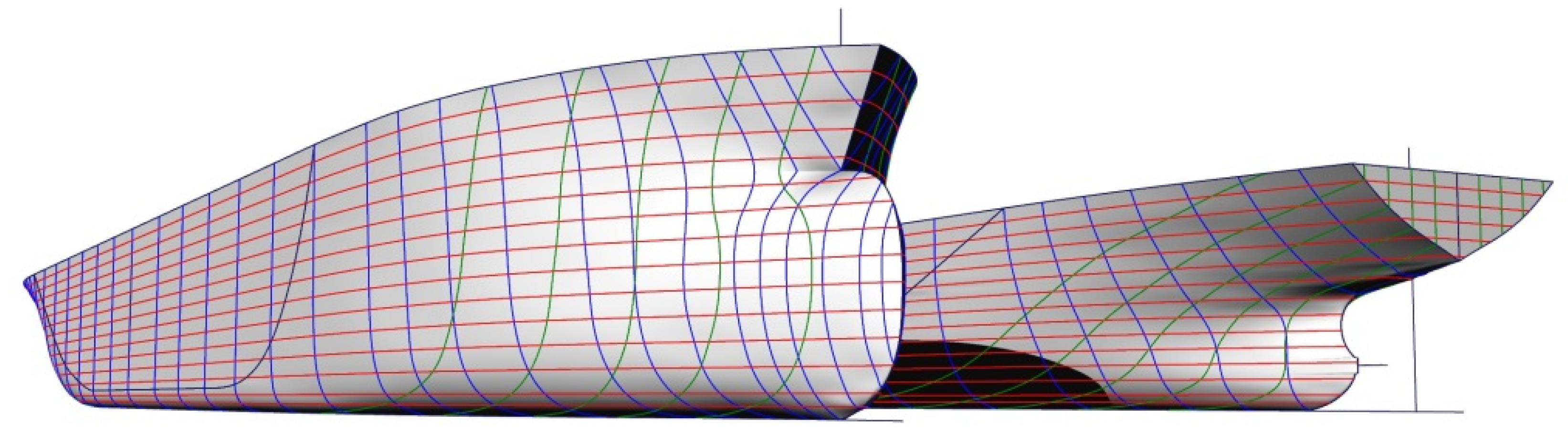
The bulk-carrier under investigation features a bulbous bow and a transom stern as shown in Figure 2. The main characteristics of the ship are shown in

Table 2. Characteristics of the ship.

Length between Perpendiculars	LBP	179.595	m
Length overall	LOA	187.608	m
Waterline length	LWL	183.291	m
Beam	B	23.700	m
Draught	T	10.150	m
Displacement	Δ	37,238	tn
Block coefficient	CB	0.841
Ship Speed	US	14.82	kn
Froude number	Fn	0.180
Reynold’s number	Re	1.18 × 109

. In this Table, L_BP represents the length between perpendiculars, L_OA the length overall, L_WL the waterline length at full load condition (FL), B the ship’s beam, T the draft at full load condition (FL), Δ the corresponding displacement and C_B the block coefficient. The design speed of the ship is equal to 14.82 knots resulting in a Froude number based on L_WL equal to 0.180 and a Reynolds number equal to 1.18 × 10⁹.

3.2. Model-Scale Experiments

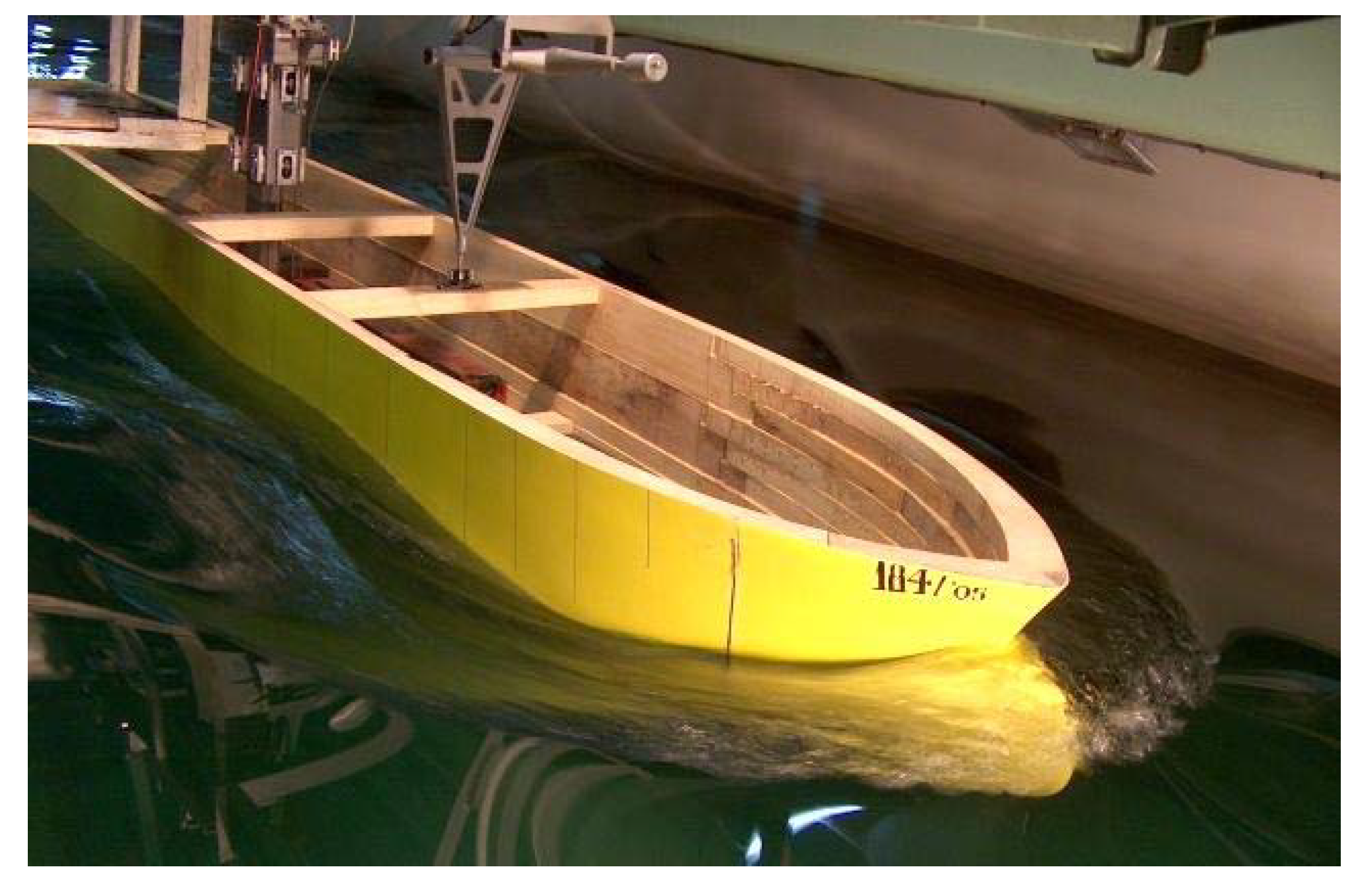
In order to evaluate the resistance and sea-keeping characteristics of the ship, a λ = 1/35 scale model was constructed at LSMH. The main characteristics of the model are shown in

Table 3. Characteristics of the model.

Scale	λ	1/35
Length between perpendiculars	LBP	5.131	m
Length overall	LOA	5.360	m
Waterline length	LWL	5.237	m
Beam	B	0.677	m
Draught	T	0.290	m
Model Speed	UM	1.289	m/s
Froude number	Fn	0.180
Reynold’s number	Re	7.68 × 106

. The model was tested in various displacements, trim and speeds [19,20] but in the present work we are concerned with the full load condition and the design speed. Following the Froude scaling method, where the Froude number Fn = 0.180 is kept equal between the ship and the model, the resulting model velocity is U_M = 1.289 m/s as shown in Table 3.

All experiments were conducted at the towing tank of LSMH-NTUA. The main characteristics of the facility are presented in

Table 4. Characteristics of NTUA towing tank.

Length	90.00	m
Breadth	4.60	m
Depth	3.00	m
Maximum carriage speed	5.30	m/s

. For resistance, propulsion and sea-keeping experiments, the models are towed along the tank via a carriage that houses all measuring equipment. The model is towed via a dynamometer, measuring the drag, also allowing for two degrees of freedom in pitch and heave. The tank is also equipped with a paddle-type wave generator able to create harmonic and irregular waves with a maximum amplitude of 0.20 m and a frequency range 0.3–2.0 Hz. The experimental uncertainty has been calculated for previous resistance measurements at the towing tank of LSMH-NTUA, that utilized the same experimental setup [21]. The uncertainty interval for the resistance measurements has been calculated to be less than 2% for the highest resistance values.

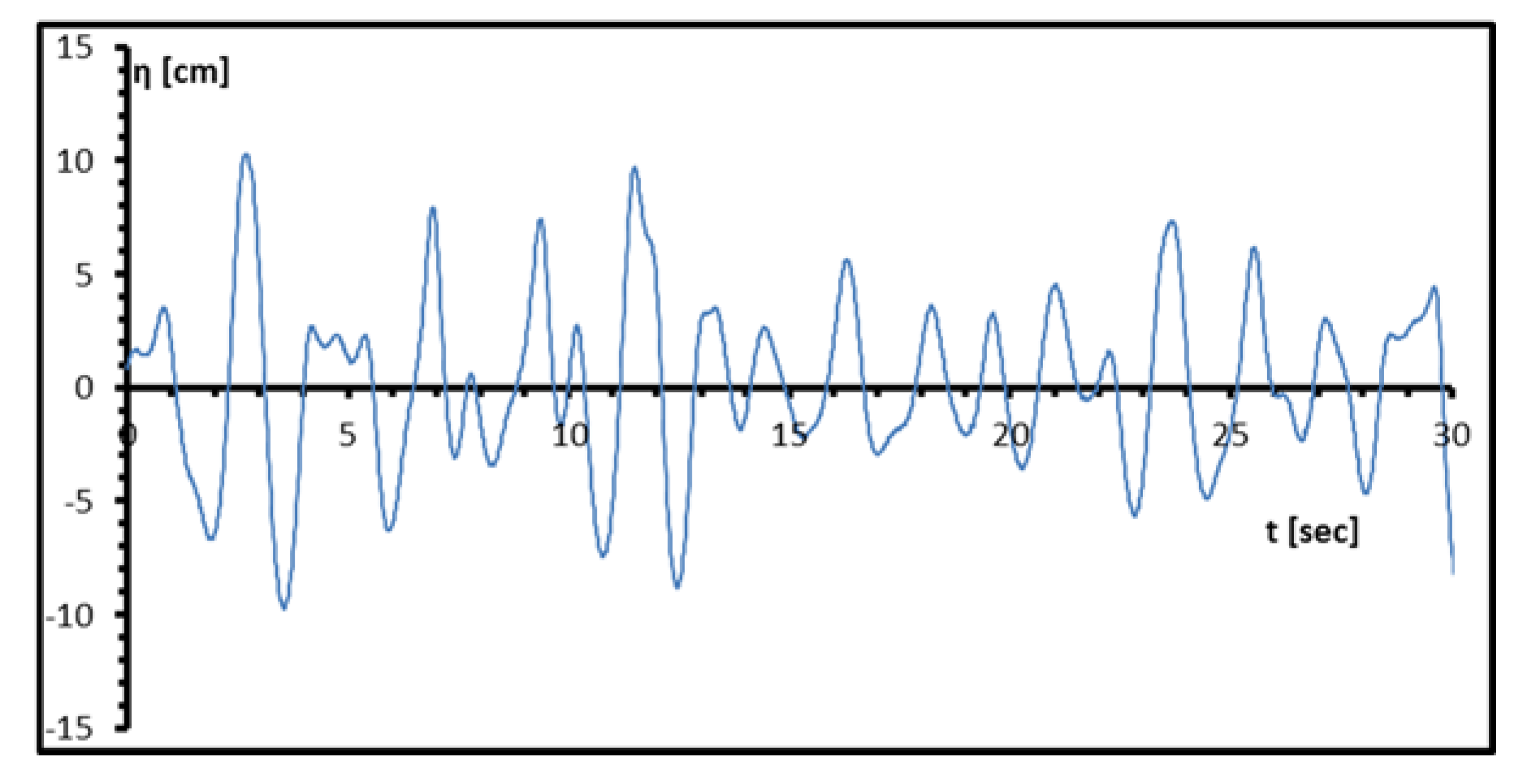
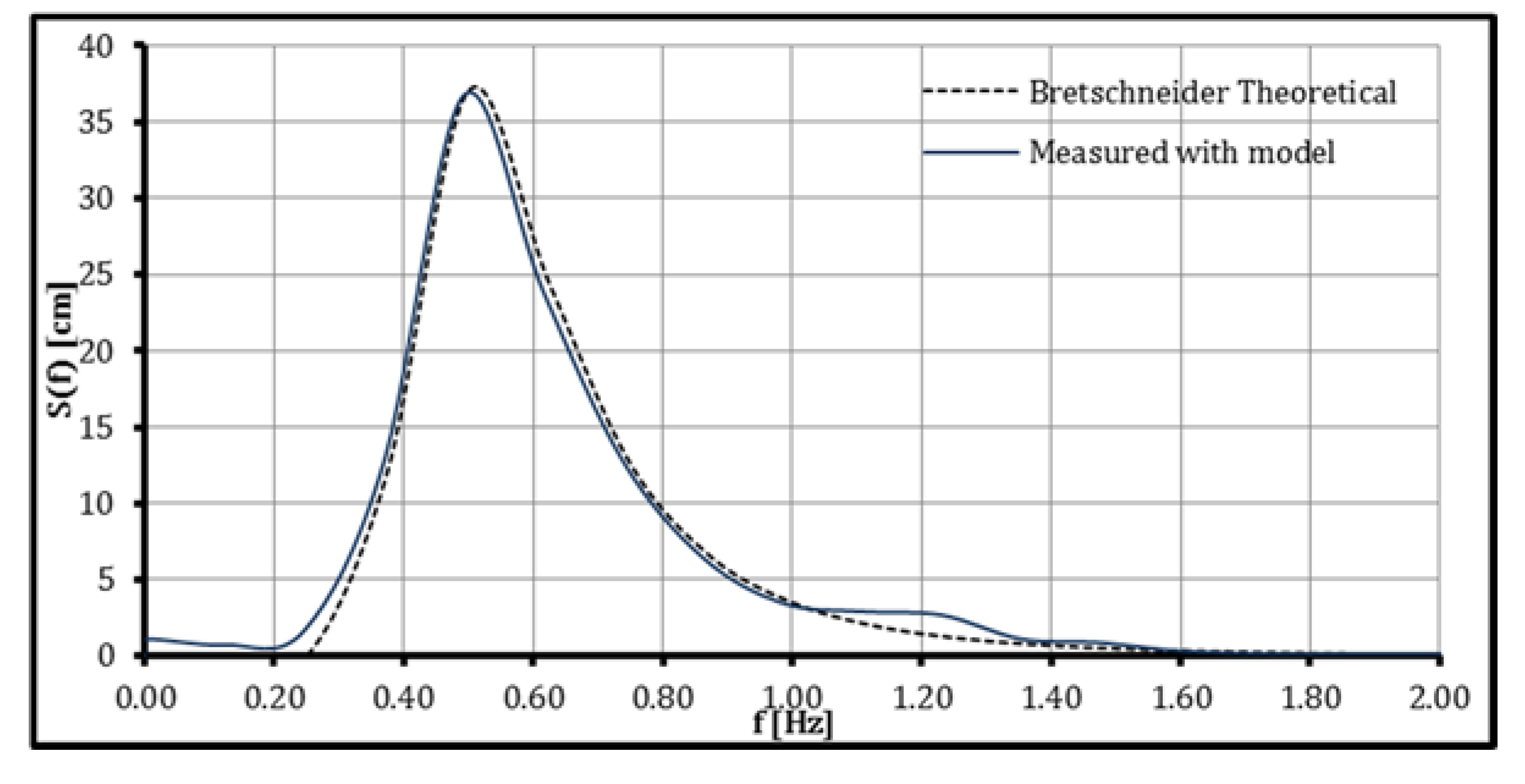
The experiments were performed previously and presented in [19,20]. Initially the calm water resistance of the model was measured. Then, the resistance and the motions of the model were measured for several incident waves, both harmonic and irregular. The waves were generated using the calibrated paddle-type wave maker. The model velocity was fixed during each measurement. In the present work, we are concerned with the case of irregular waves, following the Bretschneider spectrum [22]:

$$\begin{gathered} S(\omega )=\frac{\alpha }{{\omega }^5}\exp \left\{\raisebox{1ex}{$-\beta $}\!\left/ \!\raisebox{-1ex}{${\omega }^4$}\right.\right\} \\ \alpha =8.11\times g^2/1000 \\ \beta =\raisebox{1ex}{$3.11$}\!\left/ \!\raisebox{-1ex}{${\left(H_S\right)}^2$}\right. \\ \omega =\raisebox{1ex}{$2\pi $}\!\left/ \!\raisebox{-1ex}{$T_P$}\right. \end{gathered}$$

(14)

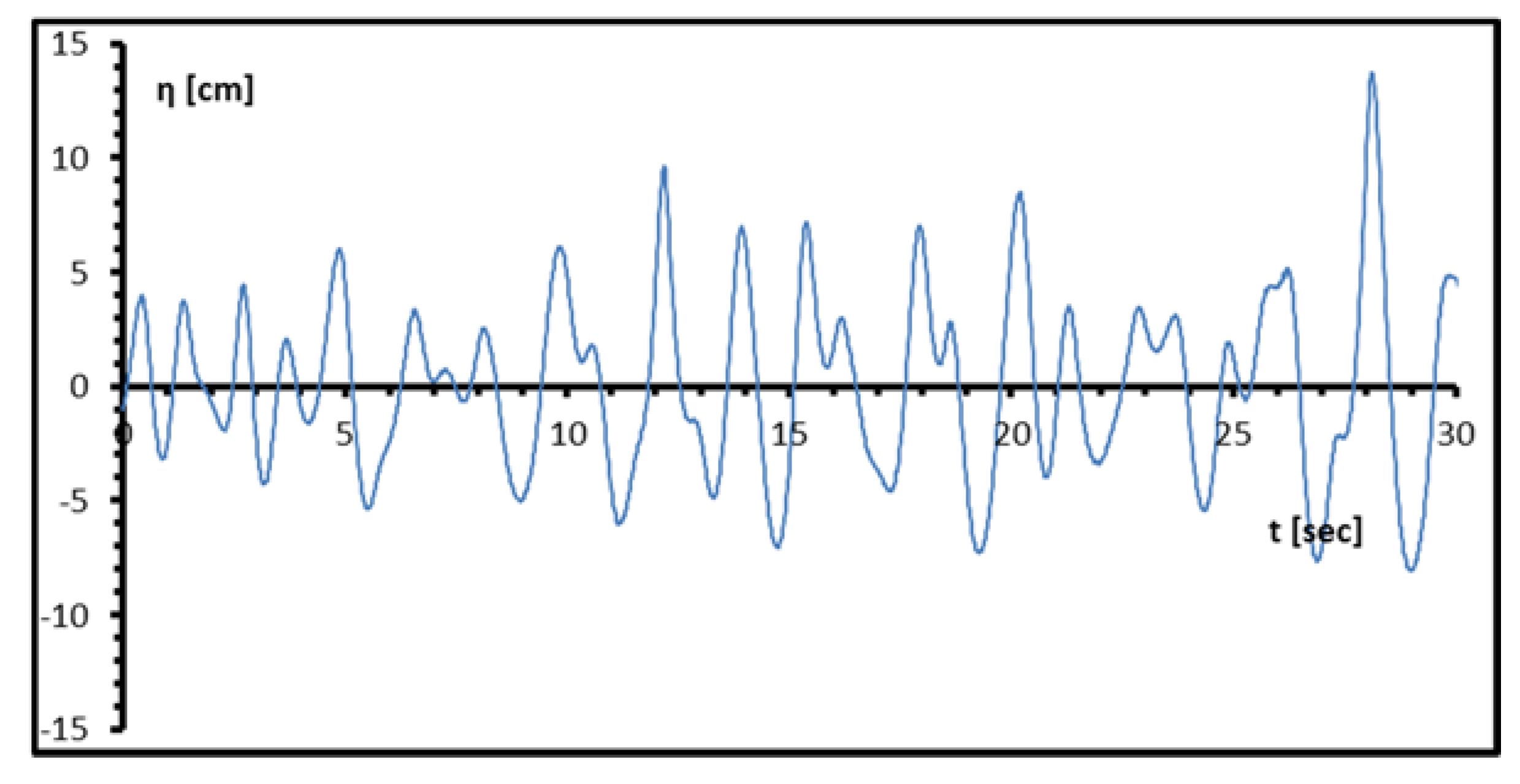
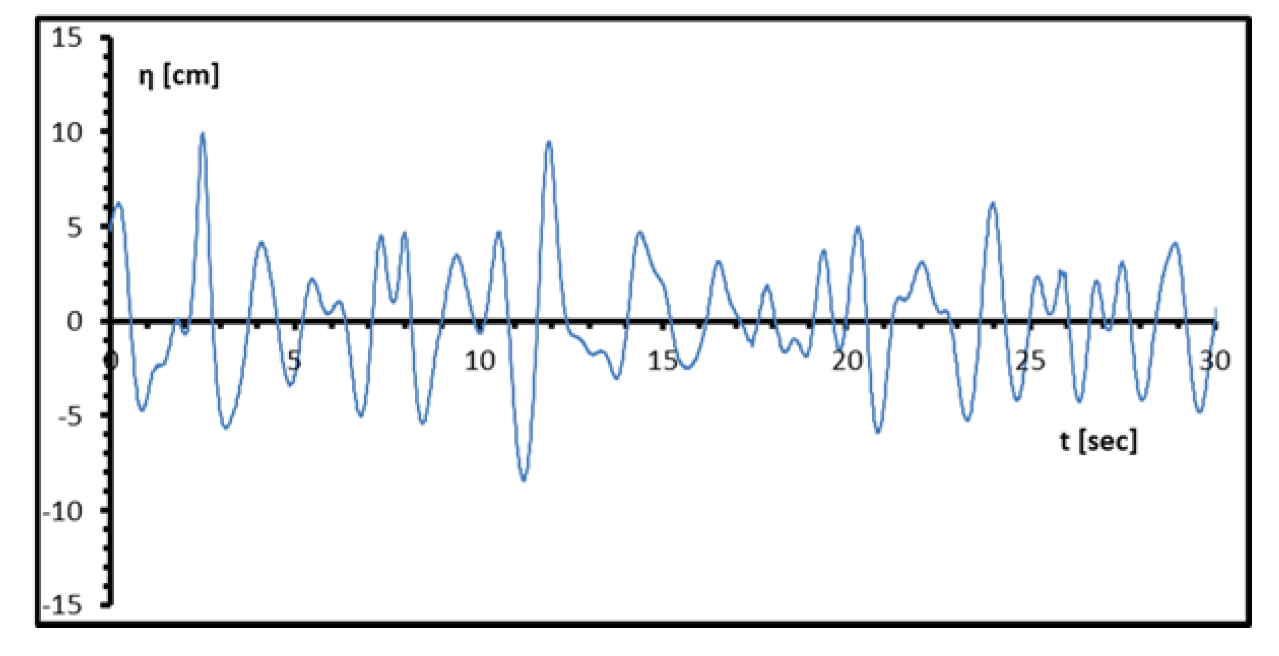
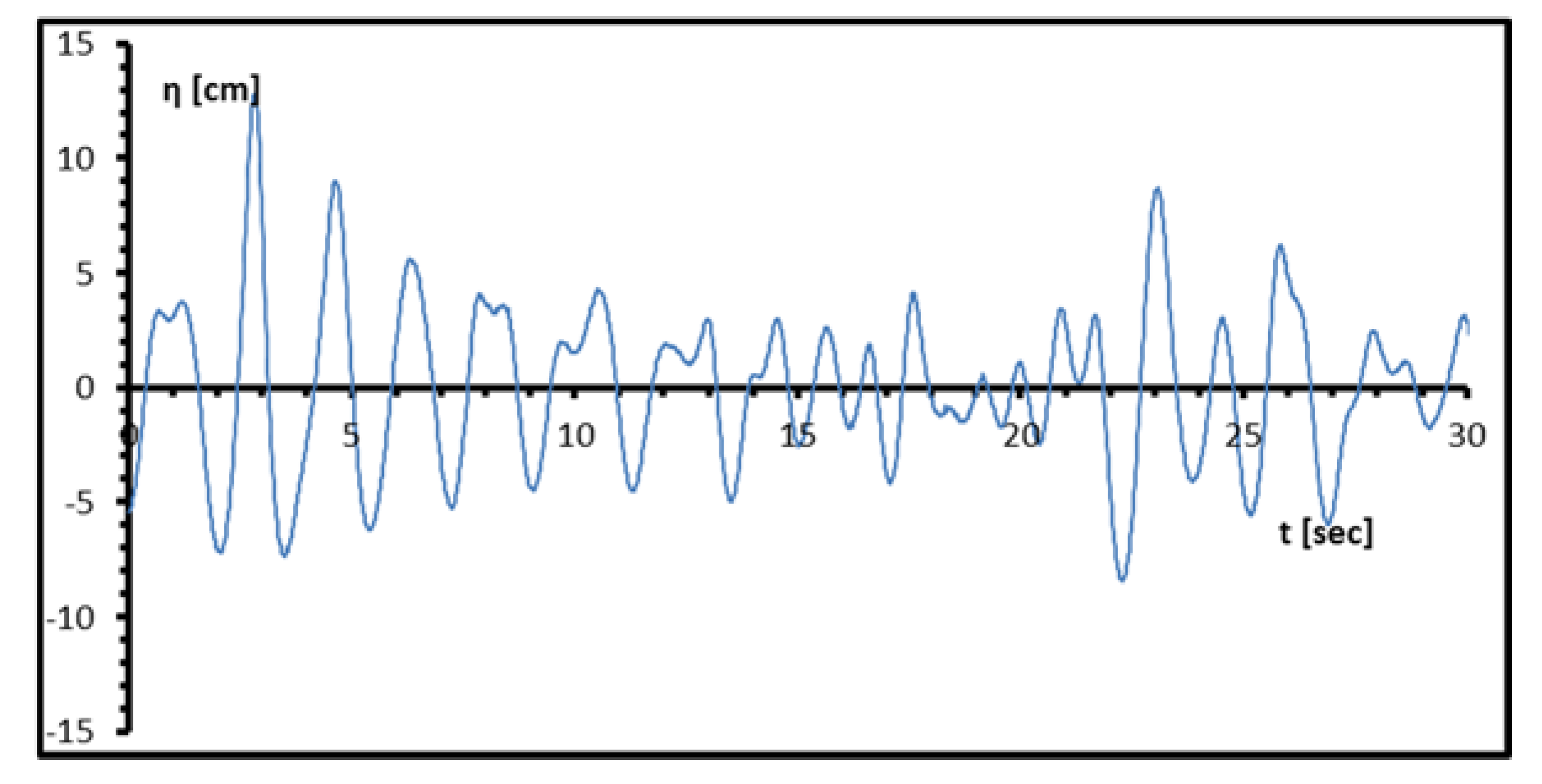
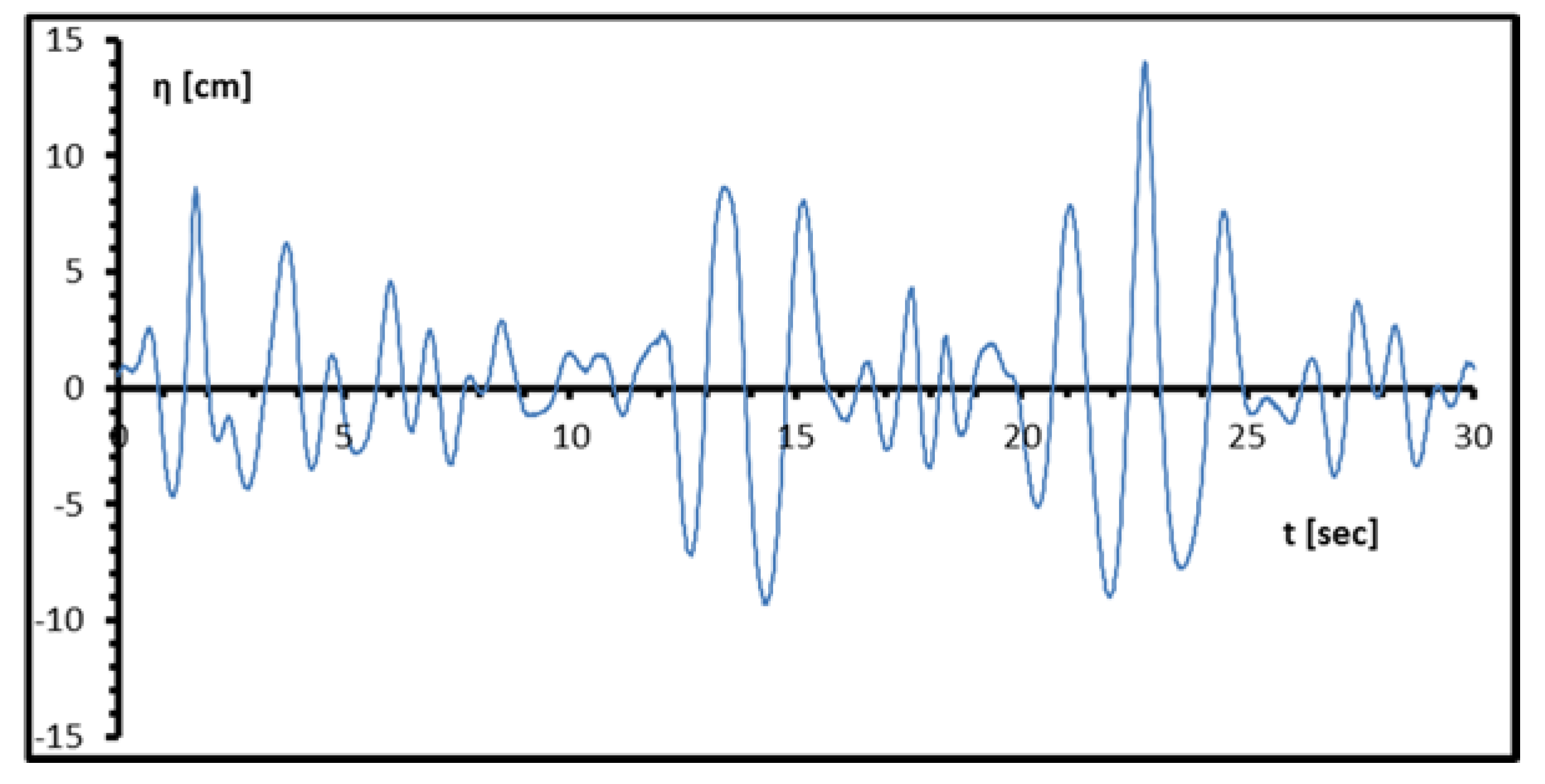
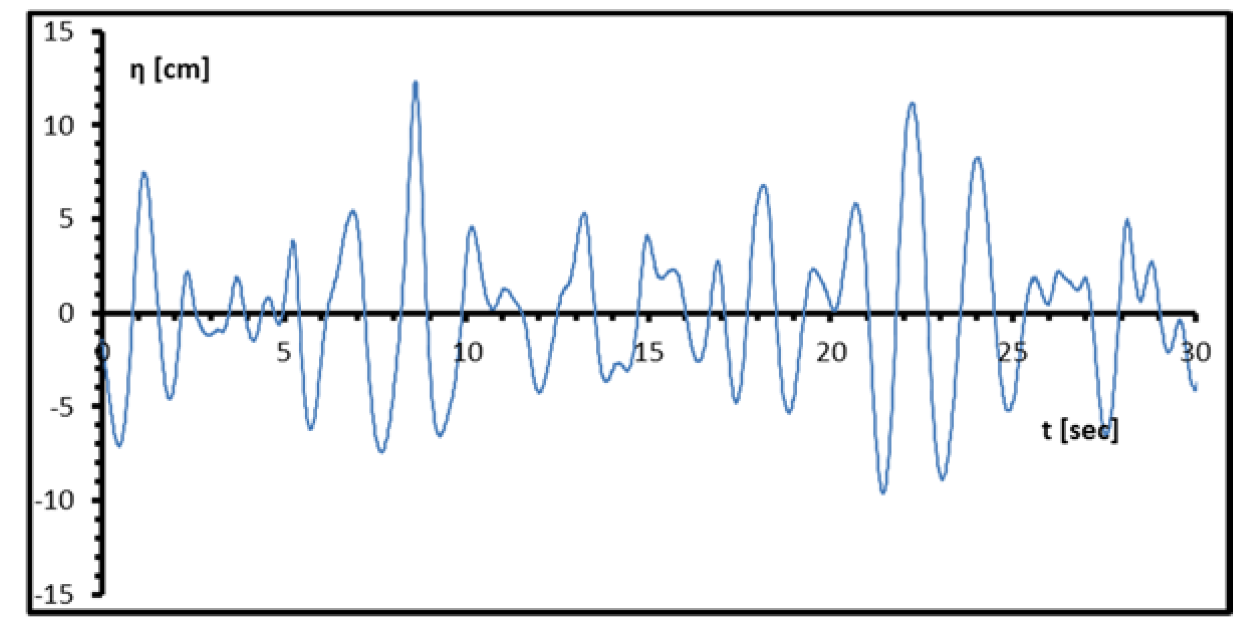
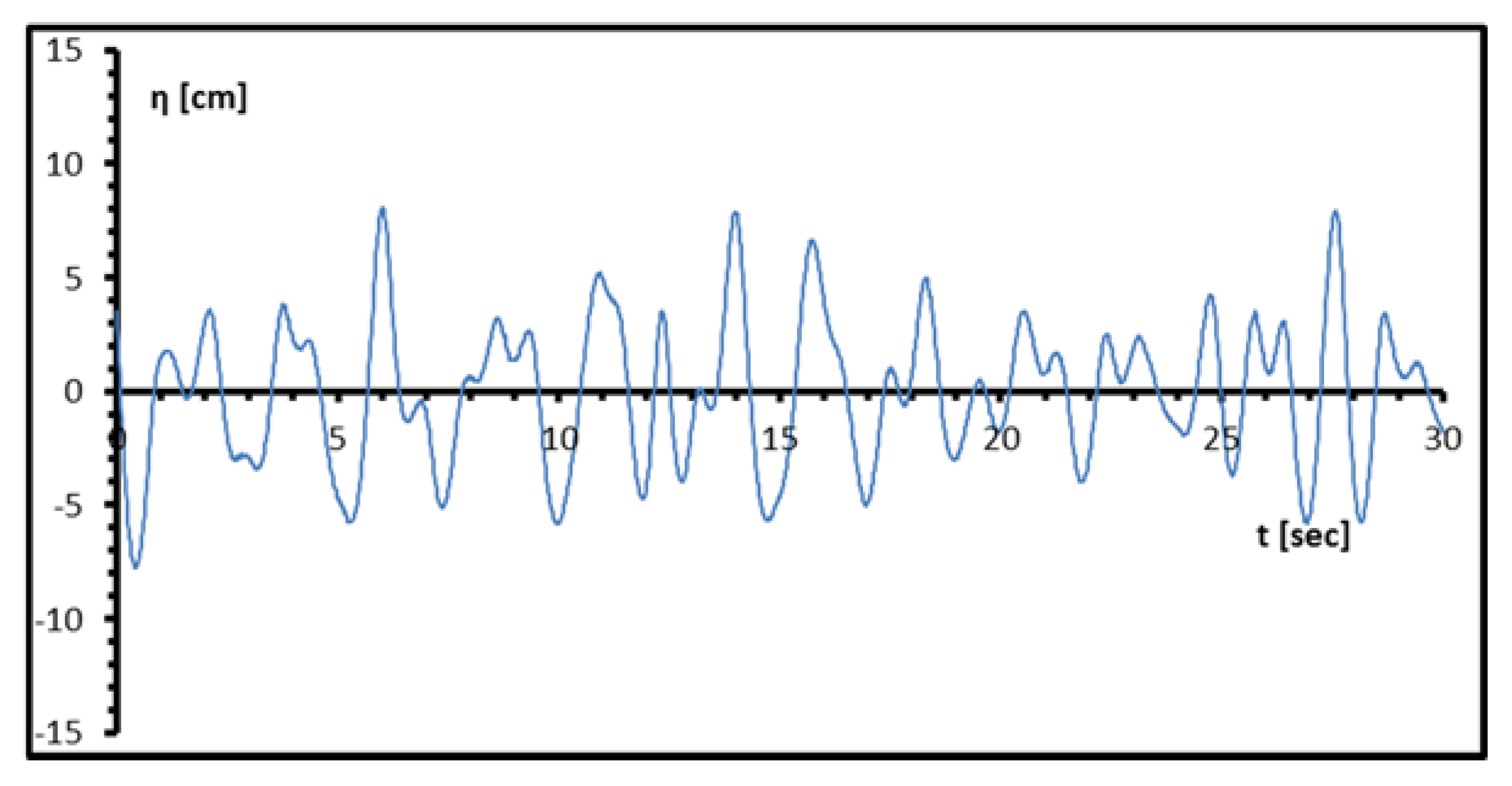
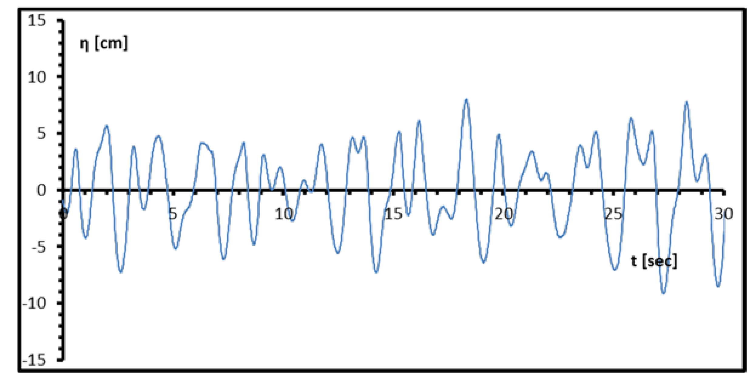
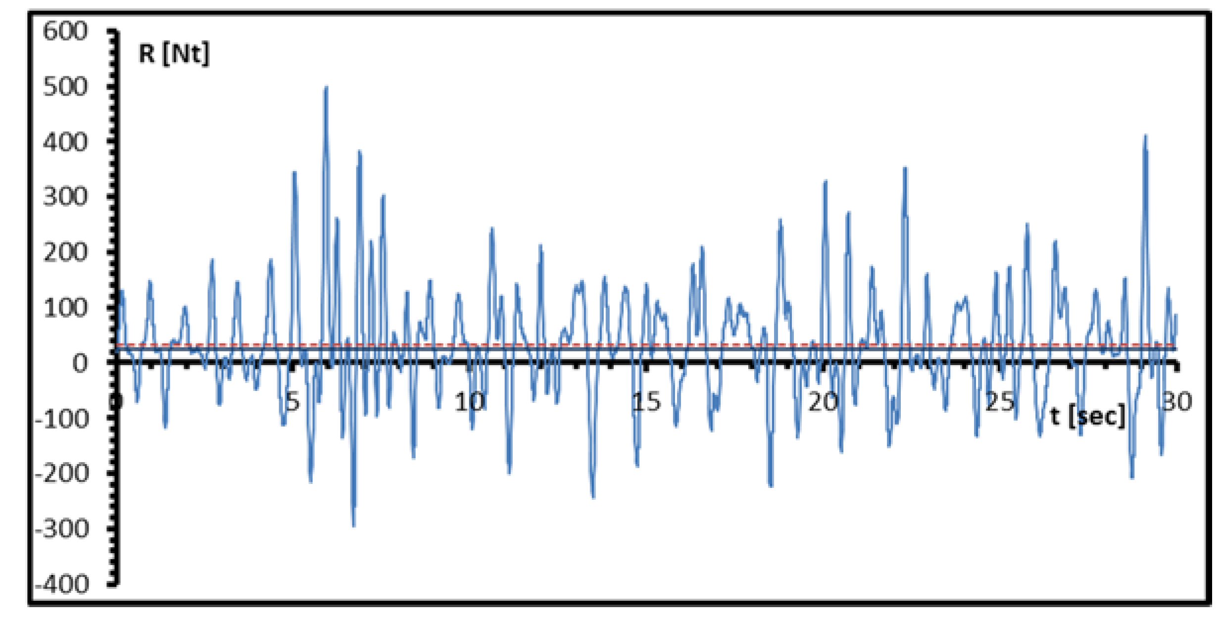
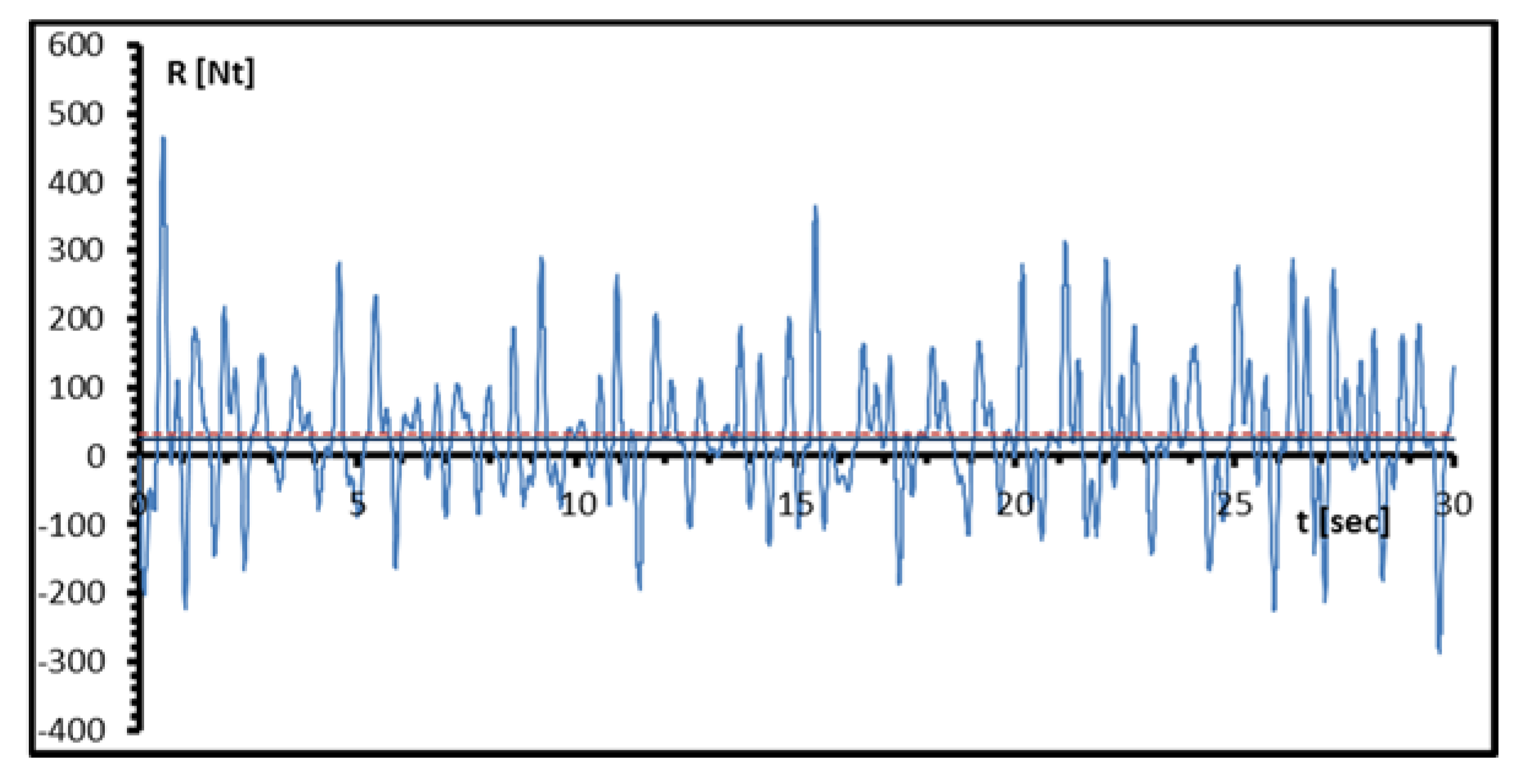
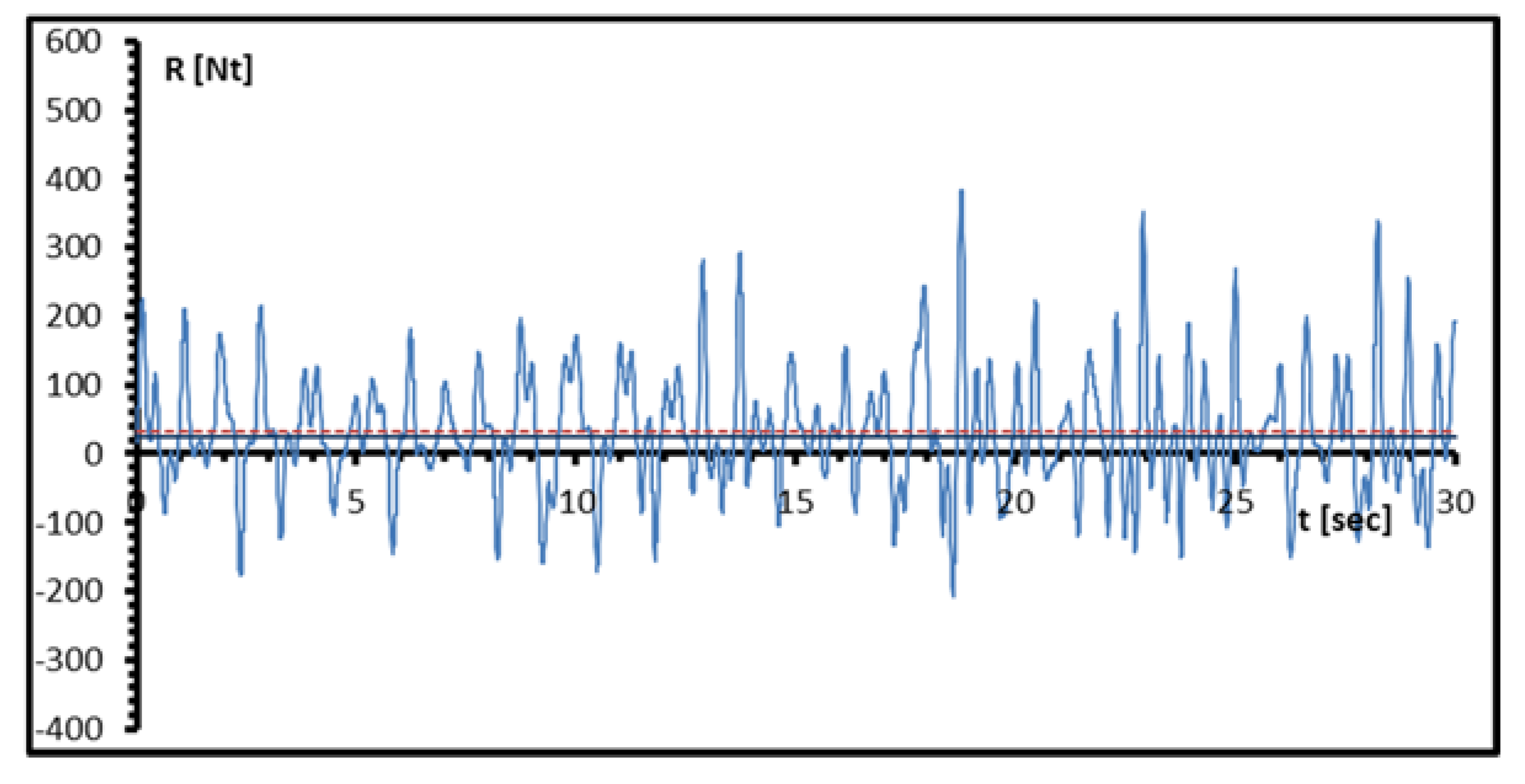
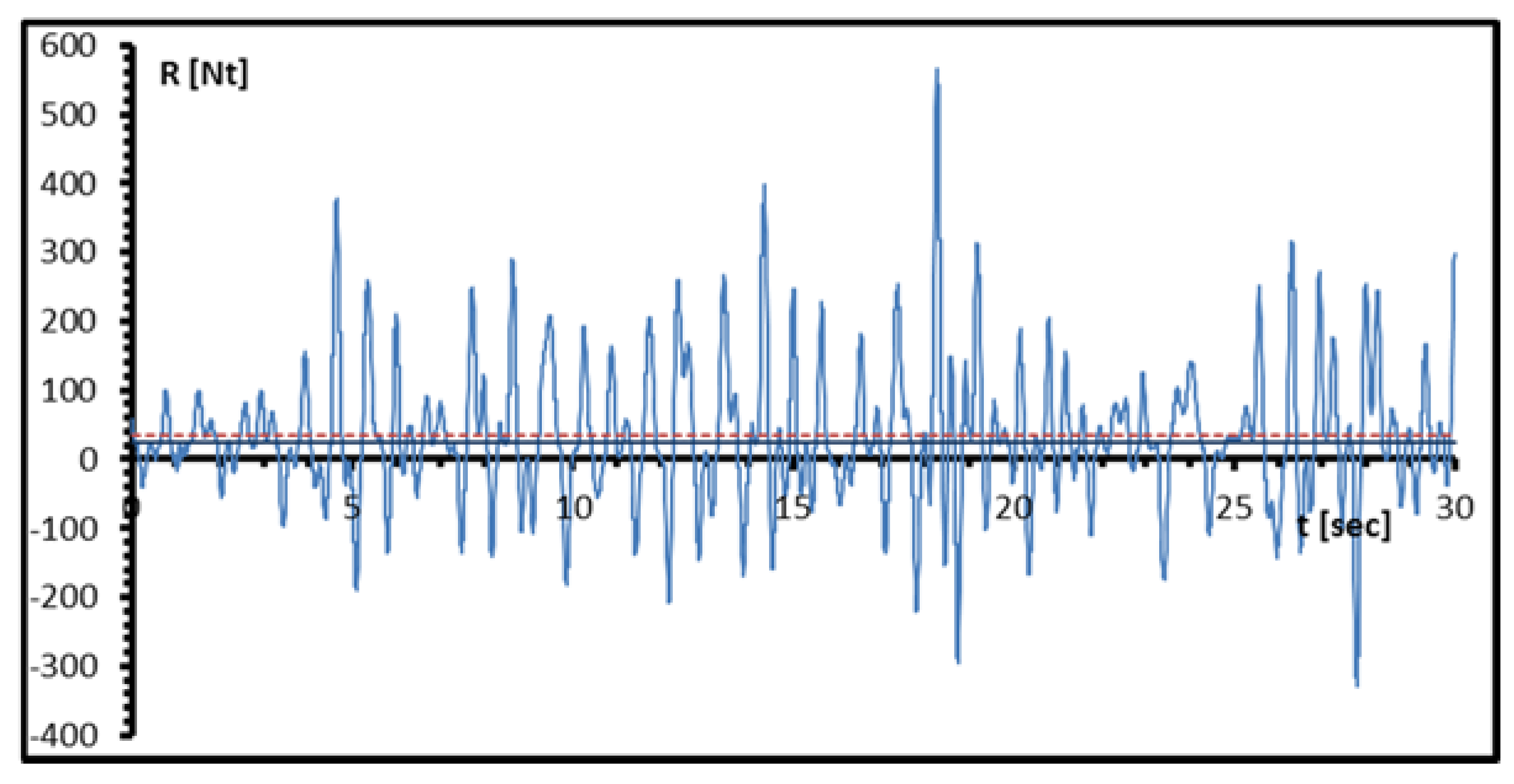
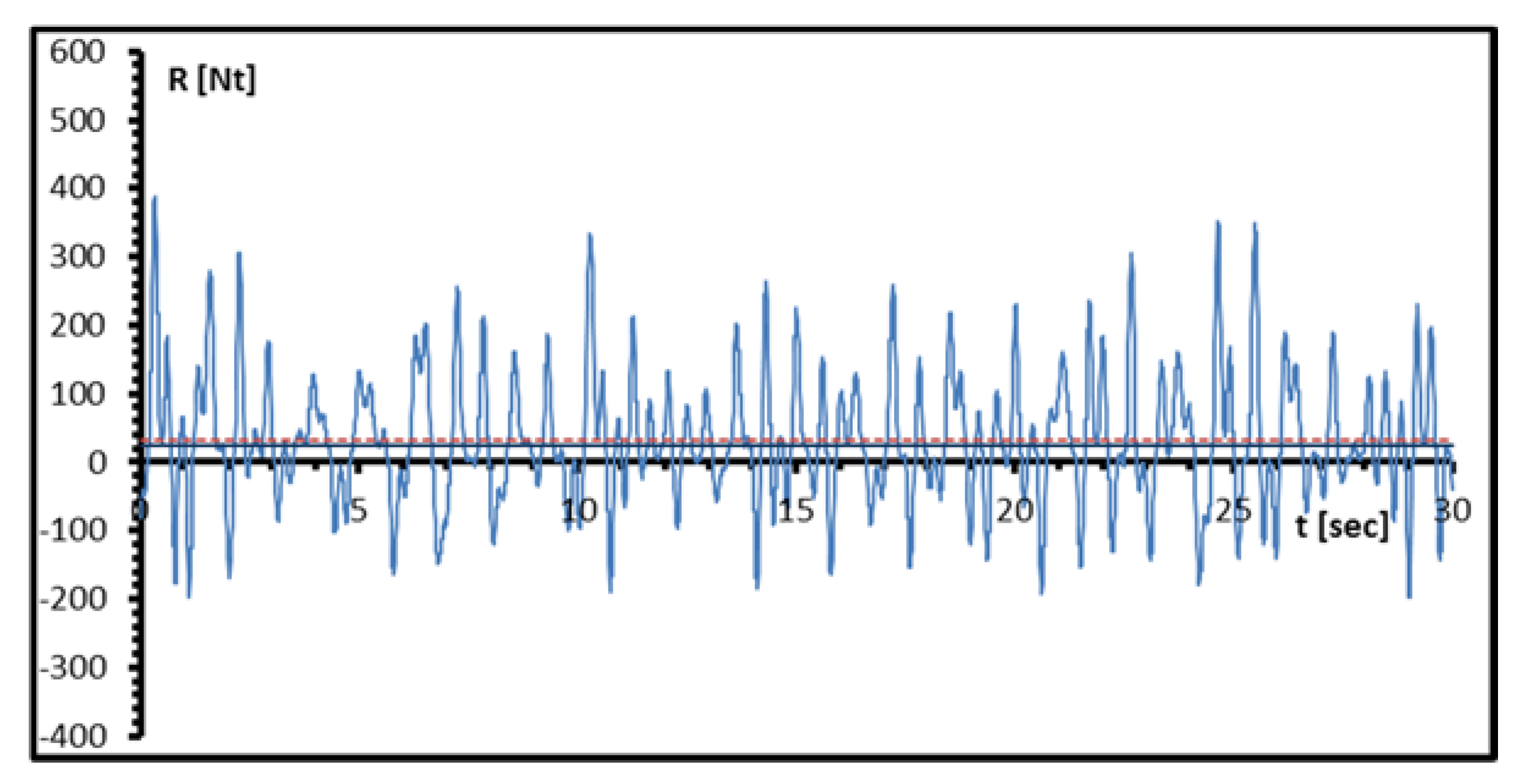
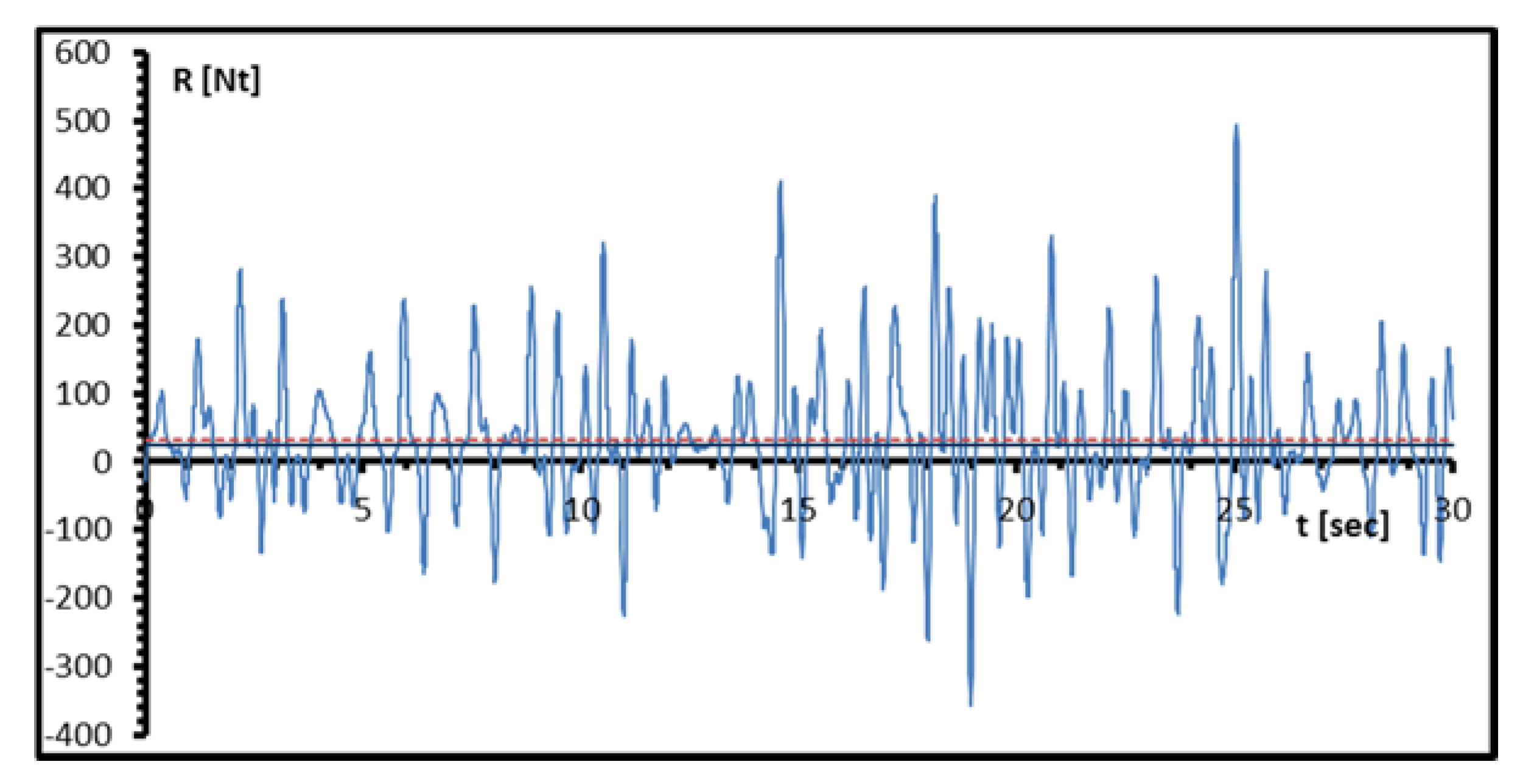
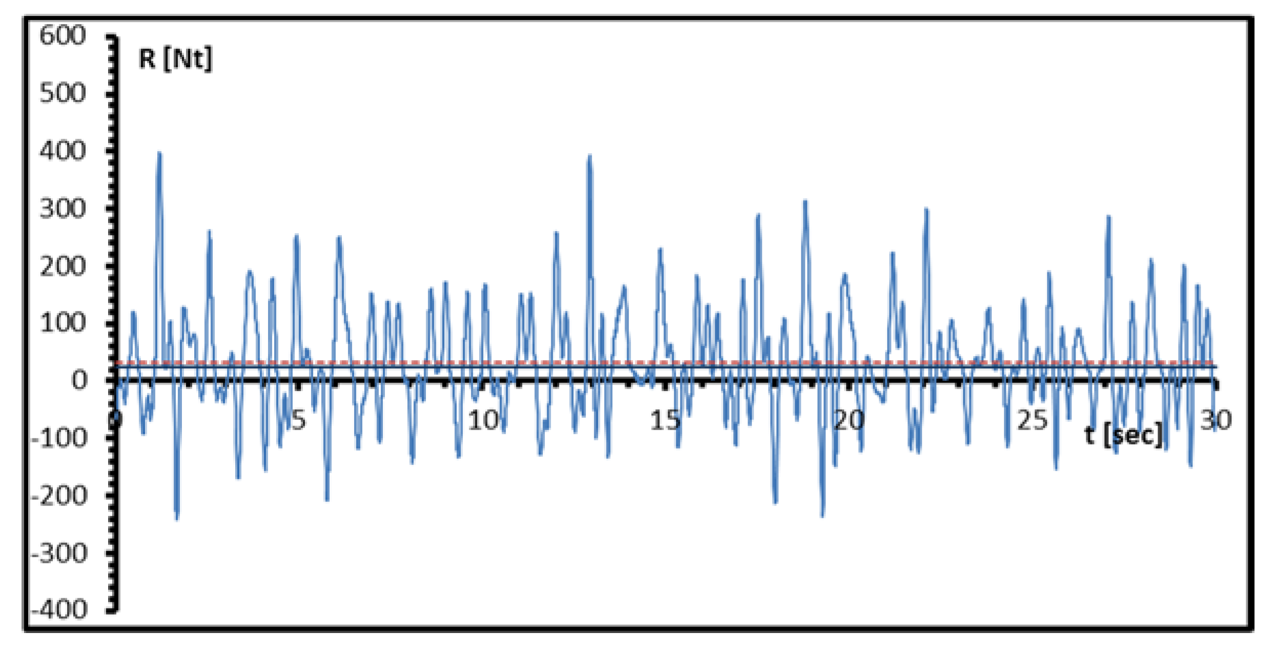
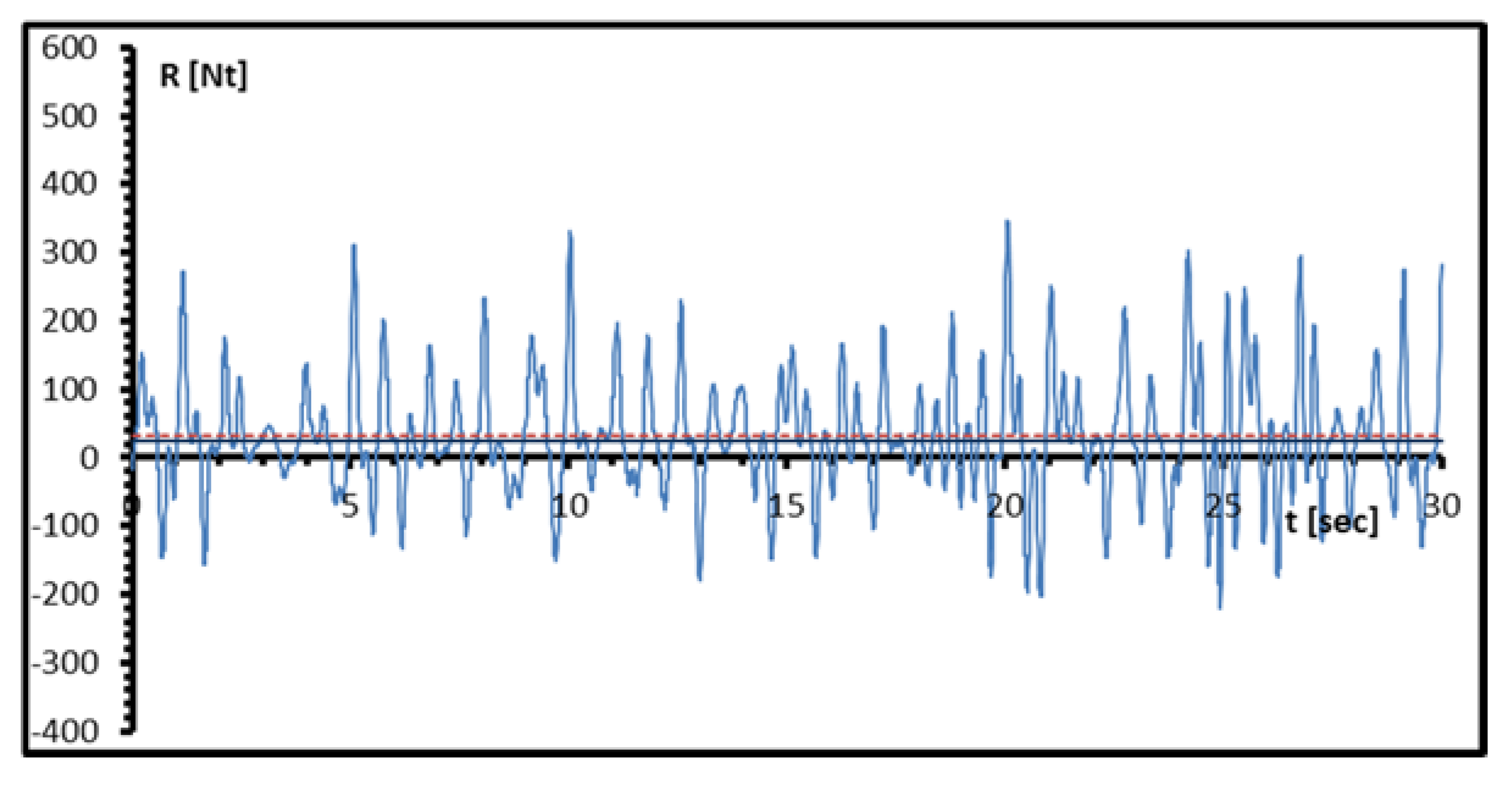
where H_S = 5.0 m is the significant wave height and T_P = 12.0 s is the spectrum peak period, both at full scale. Additionally, ω is the angular frequency, g is the gravitational acceleration, π = 3.14 and α, β spectrum shape parameters. For stochastic procedures such as irregular waves and the corresponding motions of a ship, around 20 min of recordings are required to obtain an accurate representation of all wave components. In model scale thus, the experiments have to run for 200 s. Since the total length of the tank is 90 m and the carriage needs time to accelerate and decelerate, the time of the model at a speed of 1.289 m/s is 30 s. In order to obtain enough data, the measurements were conducted in a total of eight tests each under sequential segments of a specific wave time series corresponding to the abovementioned spectrum. In Figure 3, the λ = 1/35 scale model of the examined bulk-carrier is presented during resistance measurements in the Towing Tank of LSMH-NTUA. In Figure 4, Figure 5, Figure 6, Figure 7, Figure 8, Figure 9, Figure 10 and Figure 11, the water elevation η is presented, as measured during experiments #1–#8. Finally, in Figure 12, the power density spectrum that results from the combined water elevation measurements is compared to the theoretical shape of the Bretschneider spectrum [22].

In

Table 5. Model scale resistance measurements.

Calm water resistance	RT,CW,M	24.127	Nt
Resistance in Waves, Experiment #1	RT,M,1	32.376	Nt
Resistance in Waves, Experiment #2	RT,M,2	30.937	Nt
Resistance in Waves, Experiment #3	RT,M,3	32.052	Nt
Resistance in Waves, Experiment #4	RT,M,4	33.726	Nt
Resistance in Waves, Experiment #5	RT,M,5	33.472	Nt
Resistance in Waves, Experiment #6	RT,M,6	33.199	Nt
Resistance in Waves, Experiment #7	RT,M,7	31.346	Nt
Resistance in Waves, Experiment #8	RT,M,8	31.125	Nt
Average resistance in waves	RT,M,av	32.279	Nt
Average added resistance in waves	RAD,M,av	8.152	Nt
Average added resistance coefficient in waves	CW,AD,av	1.764 × 10−3

, the measured data for the calm water resistance R_T,CW,M as well as the average value of the total resistance at waves $\overline{{\mathrm{R}}_{\mathrm{T},\mathrm{M}}(\mathrm{t})}$ are presented. Additionally, in Table 5, the calculated values of the time-average added resistance in waves and the corresponding coefficient are presented, following Equations (9) and (11).

In Figure 13, Figure 14, Figure 15, Figure 16, Figure 17, Figure 18, Figure 19 and Figure 20, the total resistance R_T,M(t) time histories are presented as measured during the experiments. The average resistance in waves, $\overline{{\mathrm{R}}_{\mathrm{T},\mathrm{M}}}$, and the calm water resistance, $\overline{{\mathrm{R}}_{\mathrm{T},\mathrm{C}\mathrm{W},\mathrm{M}}}$, are also plotted.

3.3. Computations at Model Scale

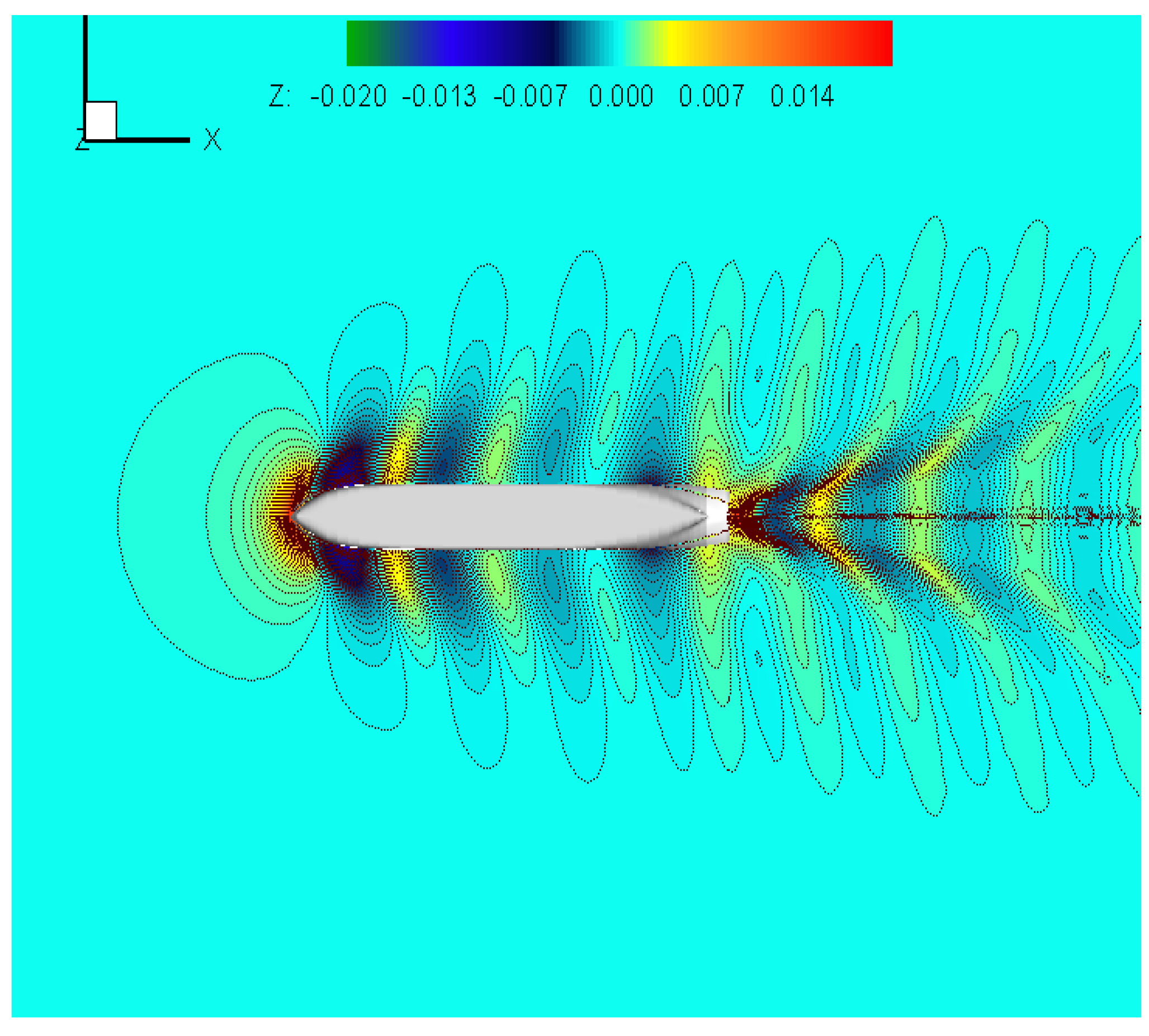
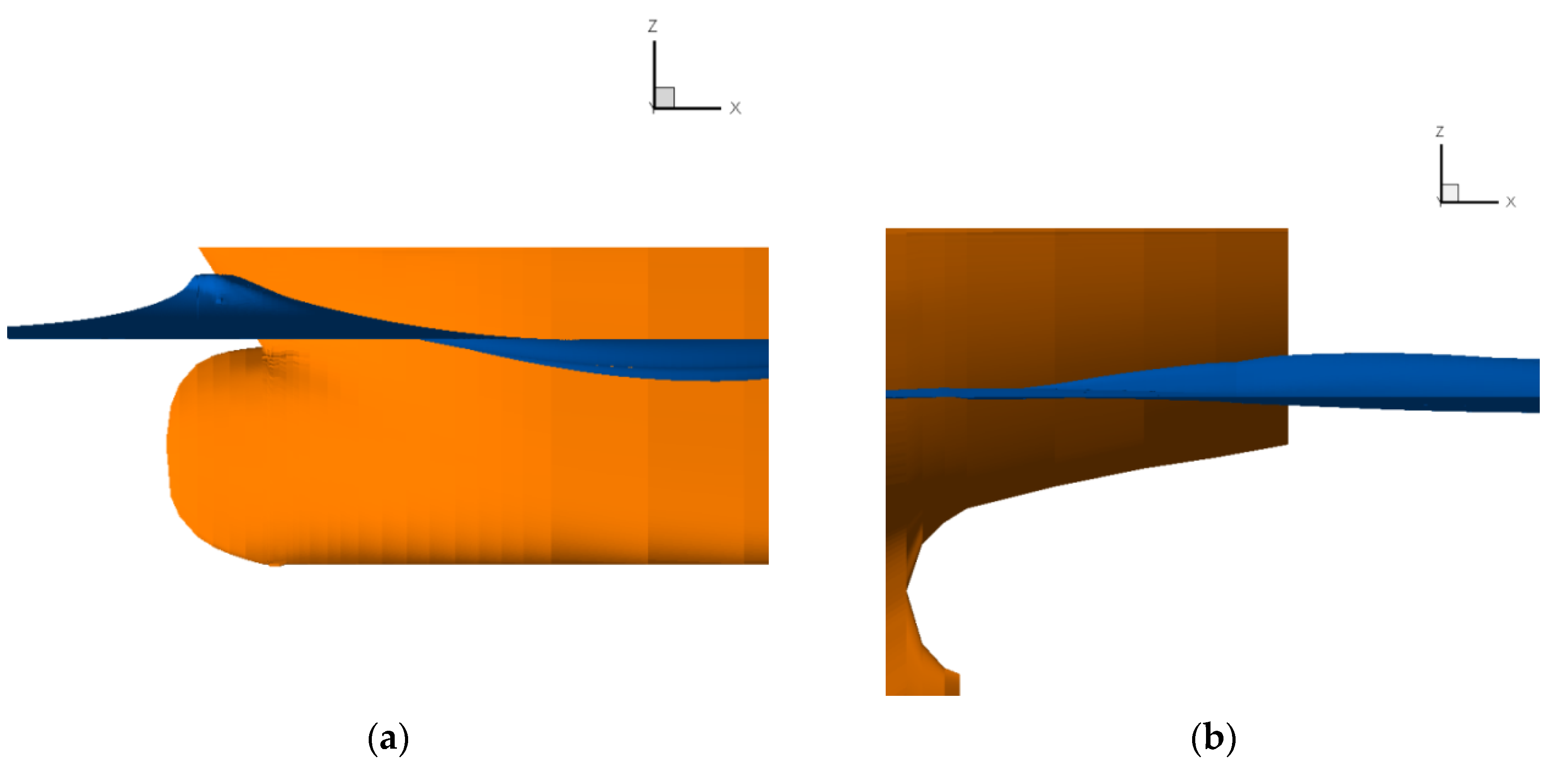
Computations at model scale were, at first, performed in order to validate the numerical method with respect to the calm water resistance experiment in the towing tank. Since the hybrid method has been adopted for the calculation of the free surface, the potential flow solver was, at first, applied. The calculation domain on the free surface extended from X/L = −0.65 to X/L = 2.2, where L stands for the ship’s length and X = 0 at the fore perpendicular. Besides, the external boundary was placed at a distance equal to L from the center line. A total number of 46,000 quadrilateral elements were used, of which 35,000 covered the free surface and 11,000 the wetted surface of the ship. During the calculations, the ship was free to sink. Once the potential solution has been accomplished, the viscous flow code has been applied in order to predict the free boundary around the transom stern and the wake region, in model-scale, thus obtaining a free surface corrected for the viscous effects at the stern. The same external boundaries were used in the computations, while the common boundary between the two solutions located at X/L = 0.85. The grid around the body consisted of 9.5M grid nodes, while 670 transverse sections and 180 grid points in the transverse direction were introduced. In Figure 21, the water elevation contour is presented for the ship at model scale, at a Froude number Fn = 0.180. In Figure 22, the free surface around the bow and the stern of the model is plotted.

The corrected free surface, considered now as a fixed boundary, is introduced in the potential flow code in order to calculate the velocity and the pressure components on the external boundary. Next, the viscous flow solver was employed to perform accurate resistance calculations underneath the free surface. The calculation domain extended up to X/L = 1.5, while the external boundary was placed at a distance of 0.33 L. Grid dependence tests have been conducted for three grids, in order to study their influence on the numerical solution. The grid nodes for each grid are presented in

Table 6. Characteristics of the used grids.

Grid	N1 × N2 × N3	Total No of Nodes
coarse	645 × 57 × 125 + 122 × 59 × 104	5.3442 M
medium	774 × 68 × 150 + 148 × 71 × 125	9.2083 M
fine	928 × 81 × 180 + 178 × 85 × 150	15.7994 M

, where N₁, N₂ and N₃ denote the number of nodes along the longitudinal, the circumferential and the transverse directions, respectively, whereas the second term stands for the transom grid. The coarse grid comprises about 5.344 M, the medium 9.208 M and the fine 15.799 M grid points and the ratio between the grid resolutions in successive refinements was about 1.2 in each direction.

The calculated total resistance coefficients C_F (friction), C_P (pressure) and C_T (total) with the three grids are compared in

Table 7. Calculated resistance coefficients at model scale (Fr = 0.18, Re = 7.68 × 10⁶).

Grid	CF × 103	CP × 103	CT × 103
coarse	3.226	1.918	5.144
medium	3.206	1.903	5.110
fine	3.186	1.940	5.126

and they are defined as

$${\mathrm{C}}_{\mathrm{F}}=\frac{{\mathrm{R}}_{\mathrm{F}}}{1/2\rho \mathrm{S}{\mathrm{U}}_{\mathrm{S}}^2}\hspace{1em}{\mathrm{C}}_{\mathrm{P}}=\frac{{\mathrm{R}}_{\mathrm{P}}}{1/2\rho \mathrm{S}{\mathrm{U}}_{\mathrm{S}}^2}\hspace{1em}{\mathrm{C}}_{\mathrm{T}}=\frac{{\mathrm{R}}_{\mathrm{T}}}{1/2\rho \mathrm{S}{\mathrm{U}}_{\mathrm{S}}^2}$$

(15)

where S its wetted surface underneath the fixed calm water free surface and U_S the ship’s speed, while the total resistance R_T is the sum of the friction component R_F and the pressure component R_P, i.e., R_T = R_F + R_P. The difference in C_T between the medium and the coarse grid is about 0.3% and about 0.67% between the fine and the medium, while convergence is not monotonic. Therefore, it was considered that the fine grid could be reliable for the comparison purposes. In this case, the calculated total resistance was equal to 24.426 Nt, whereas the measured at the towing tank was 24.340 Nt, resulting in a difference of 0.35% which can be considered satisfactory as regards the applicability of the employed method.

3.4. Calm Water Computations at Full Scale

Computations at full scale were, at first, conducted in calm water in order to calculate the resistance of the ship which is the reference for the following added wave resistance tests. The non-dimensional free surface was taken from the model scale calculations, assuming that the Reynolds effect on the stern waves does not play a significant role for the purposes of the present work. The Reynolds number at full scale was equal to 1.18 × 10⁹ and the same grid densities of Table 6 were examined, changing suitably the distances of the adjacent to the wall nodes to lie in the desirable region regarding the wall function approach.

Table 8. Calculated resistance coefficients at ship scale (Fr = 0.18, Re = 1.18 × 10⁹).

Grid	CF × 103	CP × 103	CT × 103
coarse	1.487	1.672	3.159
medium	1.510	1.622	3.132
fine	1.512	1.603	3.115

compares the three grid densities with respect to the integrated resistance coefficients. Unlike the model scale results, the differences in C_T appear higher mainly owing to the coarser distribution of nodes in the normal direction, since many grid points are now concentrated near the body surface were the boundary layer is thinner due to the Reynolds effect. The convergence is monotonic and the difference in C_T between the coarse and the medium grid is 0.86%, while between the medium and the fine grid is 0.55%. By applying the Richardson extrapolation as suggested by ASME [23], the uncertainty of C_T at the fine grid is estimated lower than 0.03%.

Next, self-propulsion calculations were carried out. The propeller body forces were calculated according to the lifting line approximation, as described previously, and 25 iterative steps were needed to obtain convergence of the thrust, so that it becomes equal to the ship resistance. The main propulsive characteristics are presented in

Table 9. Calculated propulsive characteristics at ship scale.

CT × 103	CF × 103	CP × 103	1-t	1-wn	1-we	DHP (kW)	RPM
3.733	1.516	2.217	0.834	0.631	0.656	7306	120.68

. By comparing the values of the resistance coefficients to those of Table 8 with the fine grid, it is evident that the increase of C_T is mainly due to the increase of C_P which is about 38%. The thrust deduction factor 1-t is influenced accordingly. The nominal wake fraction 1-w_n appears close to the effective wake fraction 1-w_e which is derived according to the open water numerical experiment, [16]. Finally, the delivered horsepower (DHP) and the propeller revolutions (RPM) are calculated by the lifting line code where the input data are the propeller thrust and the mean effective wake.

In the time-dependent computations when the added resistance is taken into account, it is assumed that the computational grid remains the same as the one examined in calm water, while only the propeller thrust changes according to the varying wave resistance. Among the deviations from the real situation that arise with this simplification, a significant problem is related to the operation of the propeller under a continuously varying wave surface. In order to explore the influence of the relevant approximation on the propulsive performance, a numerical experiment was performed by comparing two different situations: the ship moving in calm water and the double body case where the free surface is taken as a flat plane. Evidently, in the second situation the hydrodynamic resistance will be substantially lower since the wave resistance is not taken into account. Therefore, it should be interesting to calculate the propulsion characteristics of the double body, if this difference is taken as an additional load on the propeller thrust.

The grid density adopted for the double model was equal to that of the finer grid around the actual ship. Computations at full scale without propeller in operation have shown that the resistance of the double hull was about 39% lower than that of the actual ship, mainly due to the difference in the integrated pressure resistance component. Then, by adding the corresponding load on the propeller thrust, self-propulsion computations were performed and the percentage differences between the ship and the double body case, regarding the thrust, the wake fractions, the advance coefficient J, the propeller efficiency η_P, DHP and RPM are depicted in

Table 10. Differences in the propulsive characteristics between the real ship and the double body.

	Actual Ship	Double Body	% Diff.
TP (Nt)	7.8126 × 105	7.7377 × 105	0.96
1-t	0.834	0.842	−0.96
1-wn	0.631	0.634	−0.47
1-we	0.655	0.650	0.76
J	0.444	0.443	0.22
ηP	0.533	0.532	0.19
DHP (kW)	7306	7180	1.72
RPM	120.68	119.91	0.64

. It is noticeable that all these propulsive characteristics vary below 2%, indicating that the propeller thrust is the dominant parameter which affects the flow development well underneath the free surface.

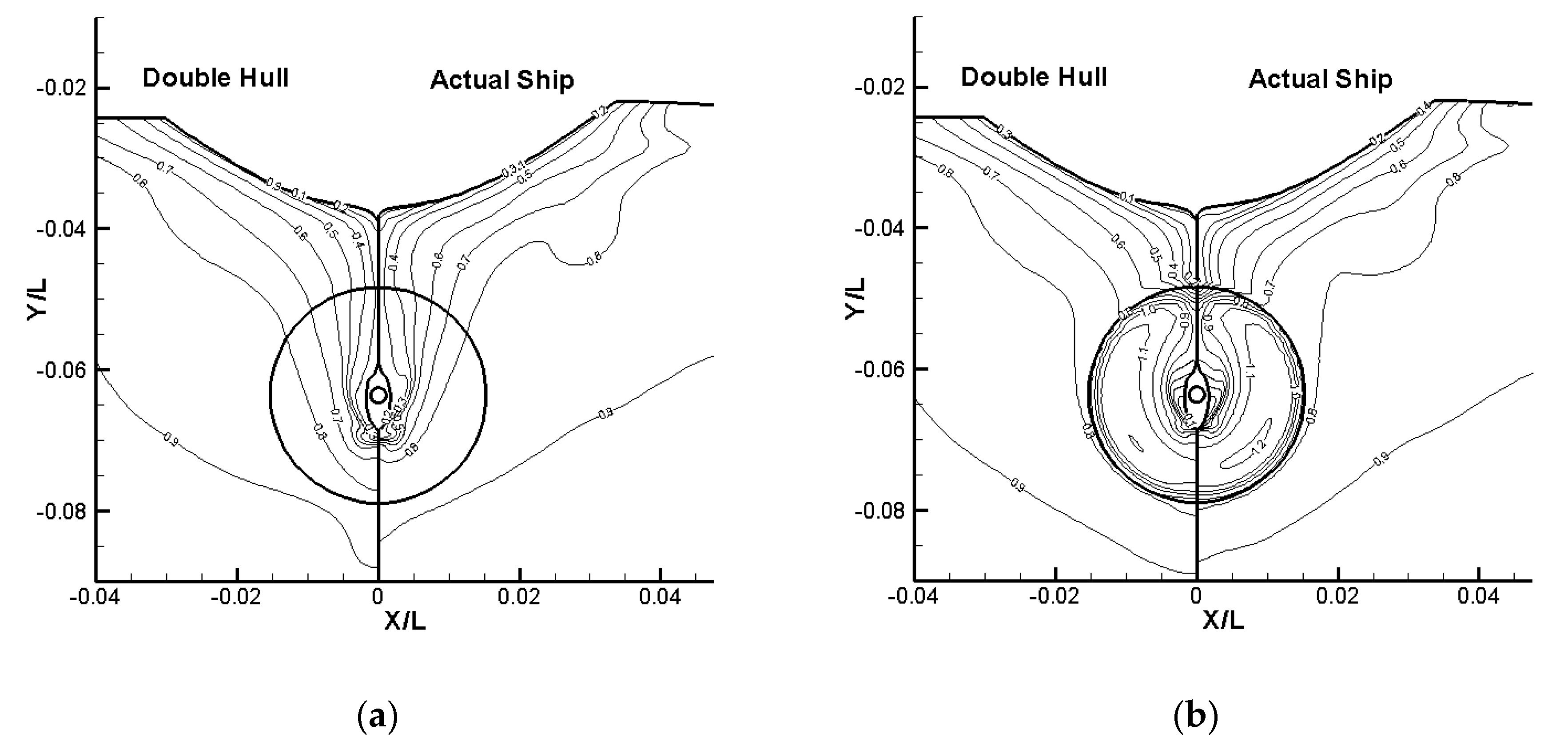
In order to support this argument, the isowakes (i.e., the ratio of the axial velocity component to the ship’s speed) on the propeller plane are plotted in Figure 23, corresponding to the computations without (a) and with propeller in operation (b). On each plot, the data on the left-hand side correspond to the double model while on the right-hand side, the data correspond to the case with free surface. Evidently, the differences between the two cases, double hull vs. free surface, are insignificant on the propeller disk, while deviations are observed close to the free surface. Therefore, these trends justify the small differences in Table 10, concerning the nominal and the effective wake fractions. Naturally, this comparison is only indicative since in reality the ship moves in random waves, which may affect more drastically the flow past the propeller.

3.5. Computations at Head Sea State

In order to study the effect of the added resistance when the ship is advancing in steady speed under random head-sea conditions, computations in the time domain have been performed following the assumptions presented in Equations (8)–(11) utilizing the resistance time series as measured in the towing tank. Thus, eight numerical experiments were conducted, each lasting 30 s. The time step in the calculations was Δt = 1 s and in each time step self-propulsion was achieved in lower than 10 iterative steps, while 15 domain sweeps were performed per iteration. Naturally, at the end of this procedure per time step, the propeller thrust equals the hydrodynamic resistance of the ship. In Figure 24, corresponding to the numerical experiment #1, the time histories of the thrust coefficient C_T = (T_P/(0.5ρSU_S²)) and the added wave resistance C_W = (C_W,AD(t)) are plotted. Evidently, C_T follows the variations of C_W but their difference is not constant, since the thrust deduction factor varies in time. It should be noticed here that a cut-off for the negative thrust components is applied, since negative thrust values imply reverse propeller operation which is impossible in real life. Thus far, the results depend on the approach of the actuator disk and represent the “real” effects under the basic assumptions of the proposed method.

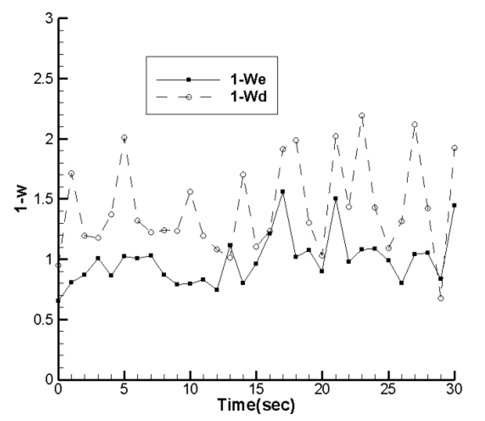
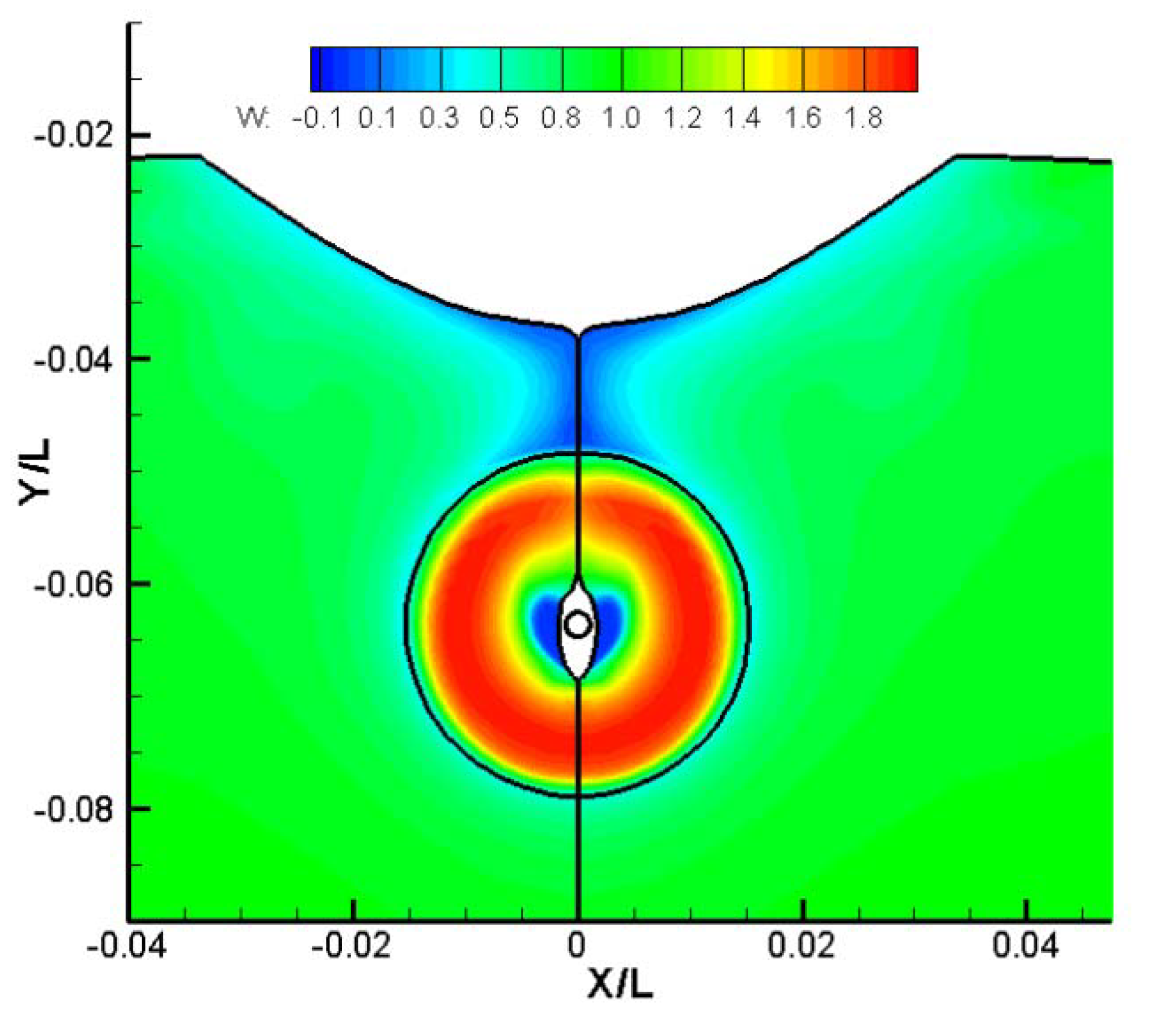
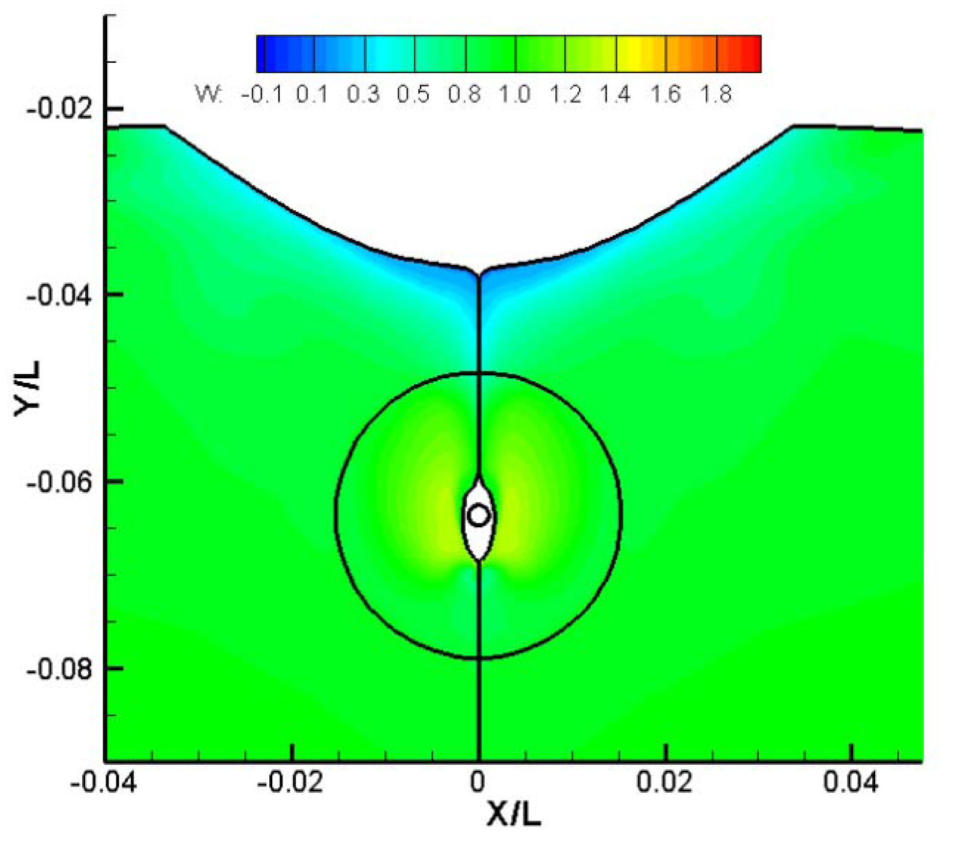
Next, the quasi-steady approximation is followed in order to estimate the powering demands. In Figure 25, the flow rate through the propeller disk 1-w_d and the effective wake fraction 1-w_e are plotted versus time. The first one is the direct result of the solution of the RANS equations, while the second one is found by an open-water numerical experiment, so that the velocity at infinite produces w_d through the disk under the known T_P [16]. Apparently, the two curves do not present the same trends, while 1-w_e is always lower, as expected, than 1-w_d. Besides, 1-w_d exhibits unusually high values, which are due to the high values of the added wave resistance and their memory effects. In any case, 1-w_e and T_P are the crucial parameters being the input data in the lifting line code or in the open water propeller characteristics whenever they are available. In Figure 26 and Figure 27, the isowake contours that are associated with the calculation of the fraction w_d are plotted correspondingly for a local maximum and a local minimum of the added wave resistance component. Evidently, the thrust following the resistance history affects drastically the wake field and enhances strongly the axial velocity component when it takes high values.

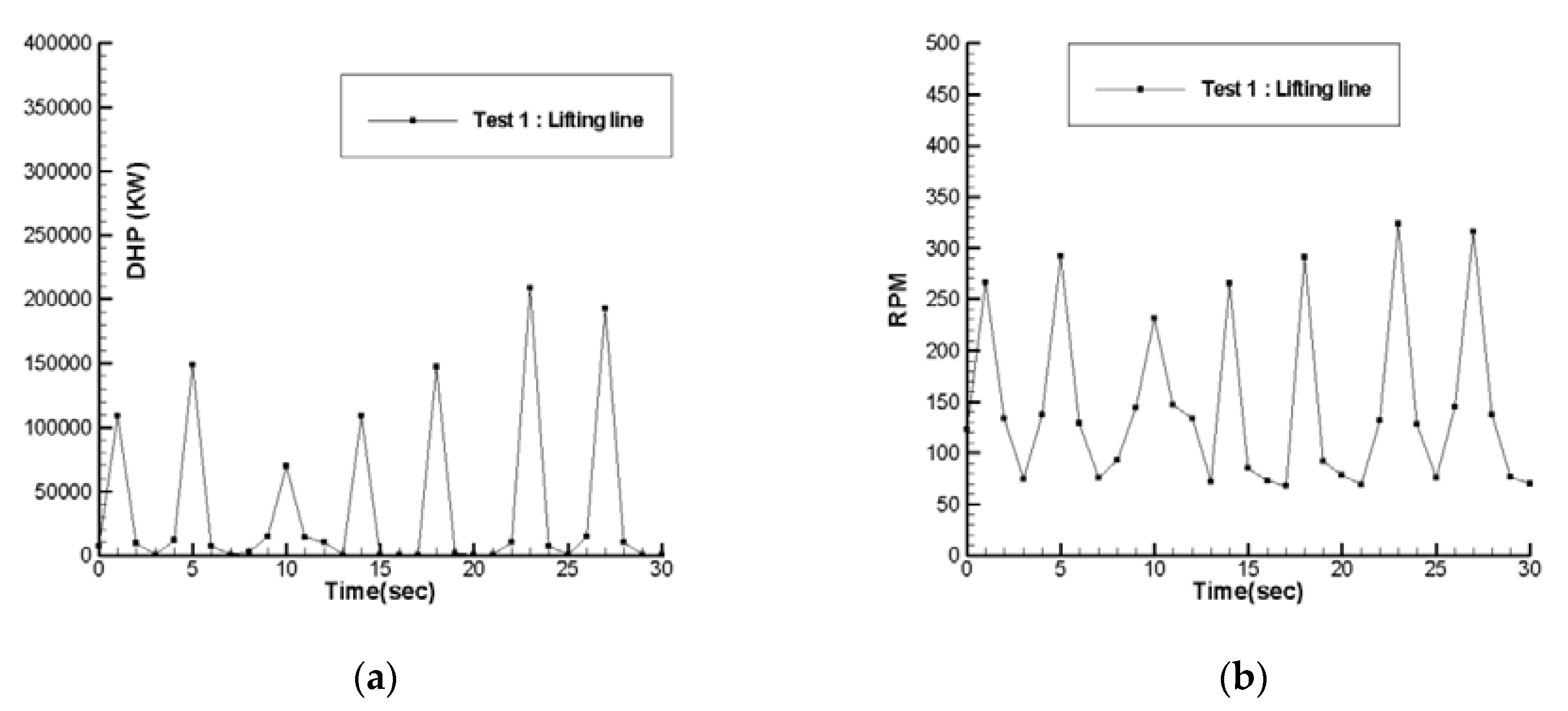
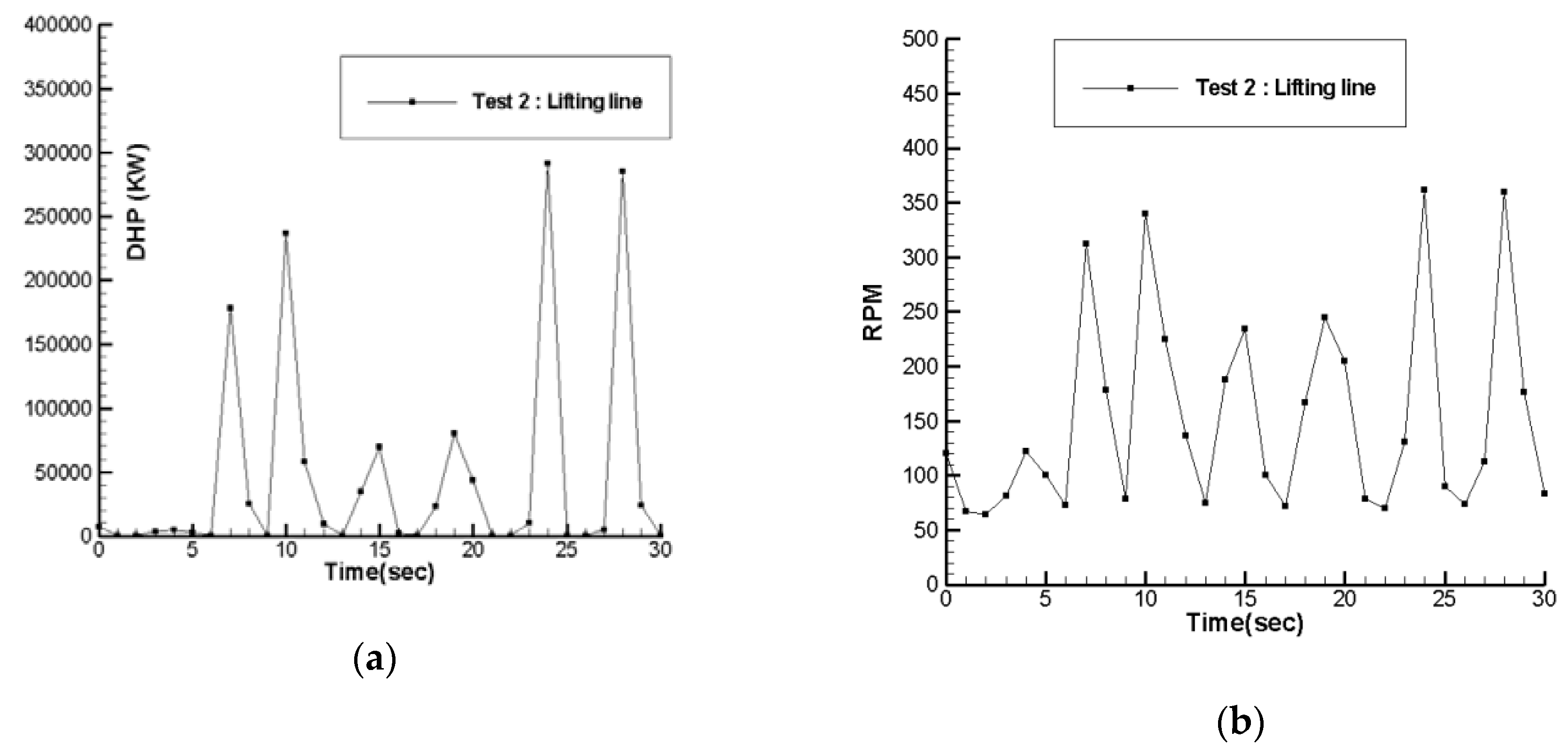
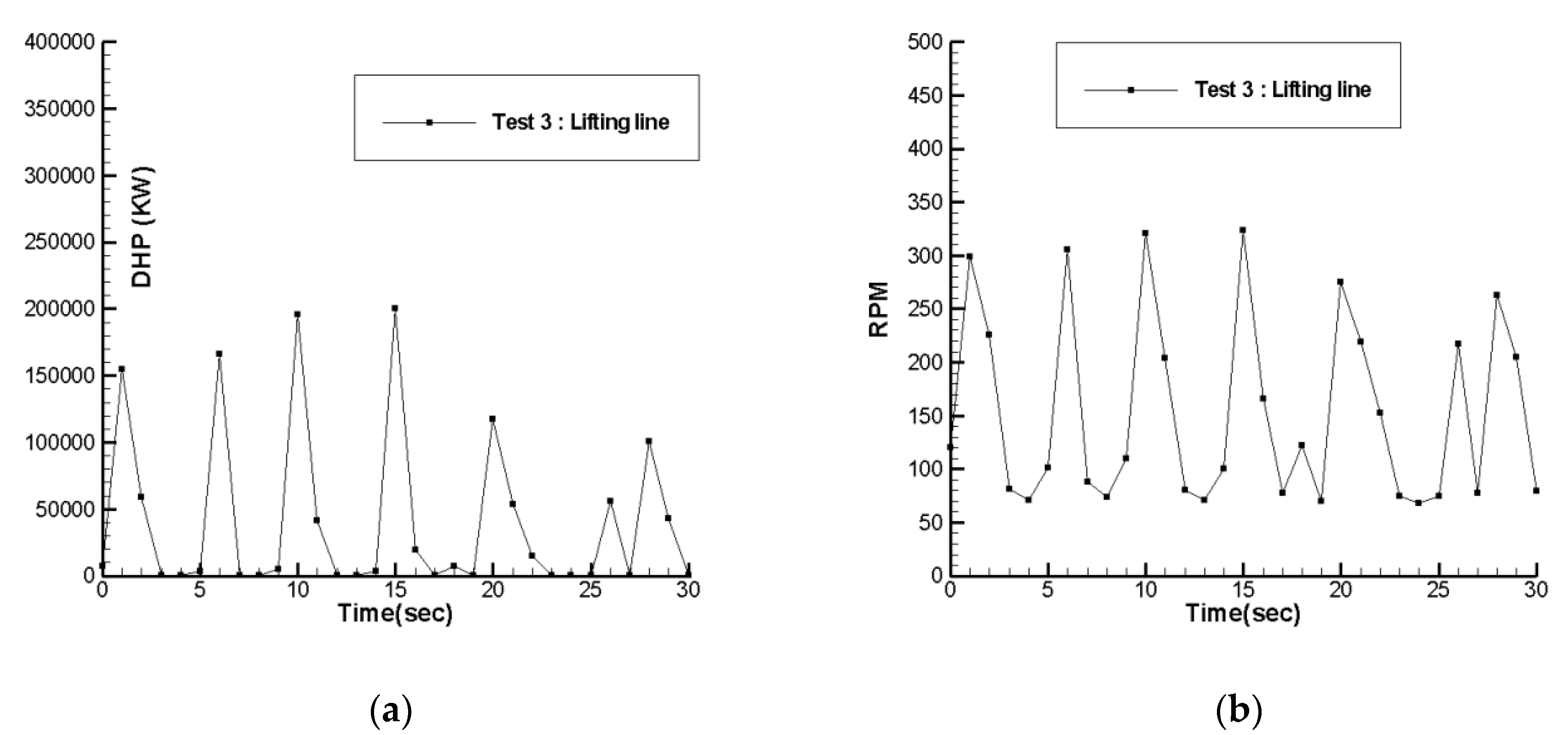
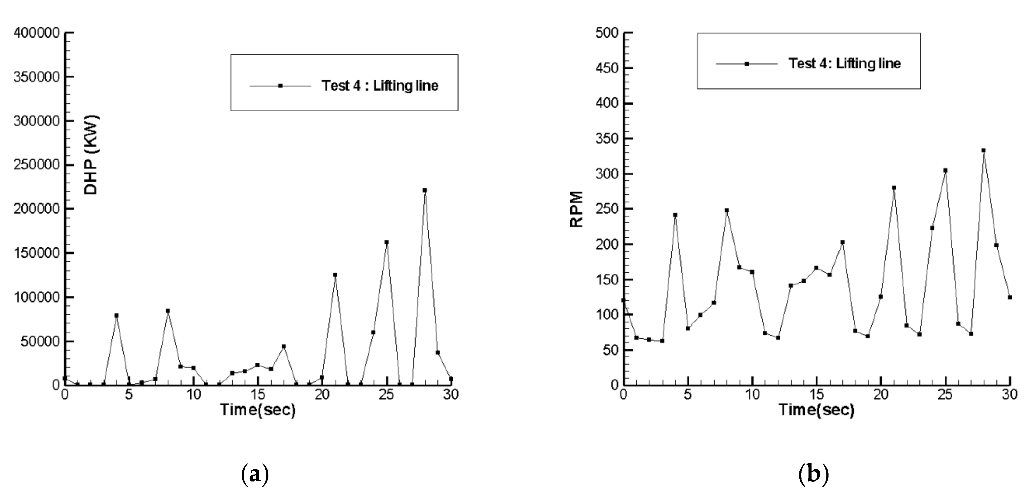
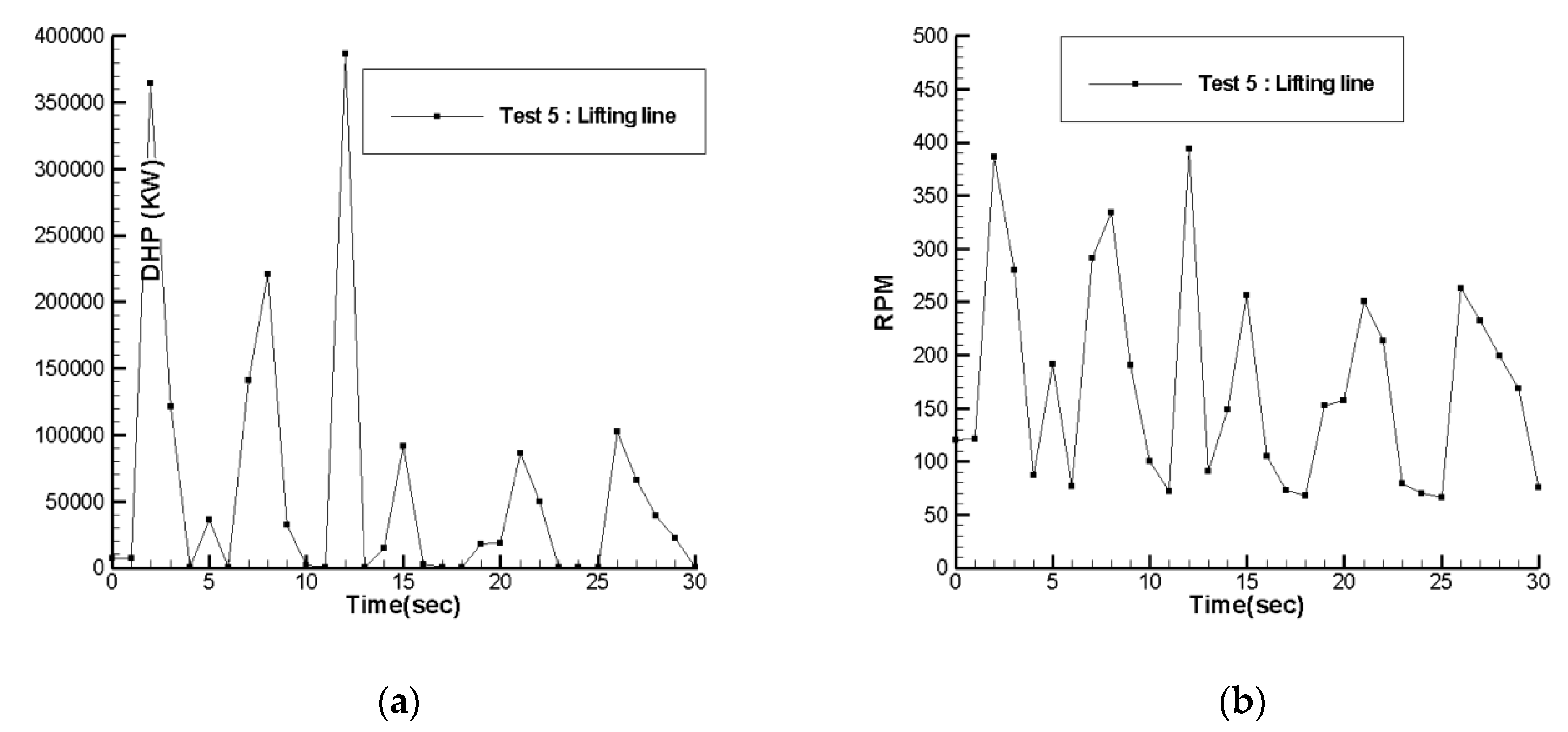
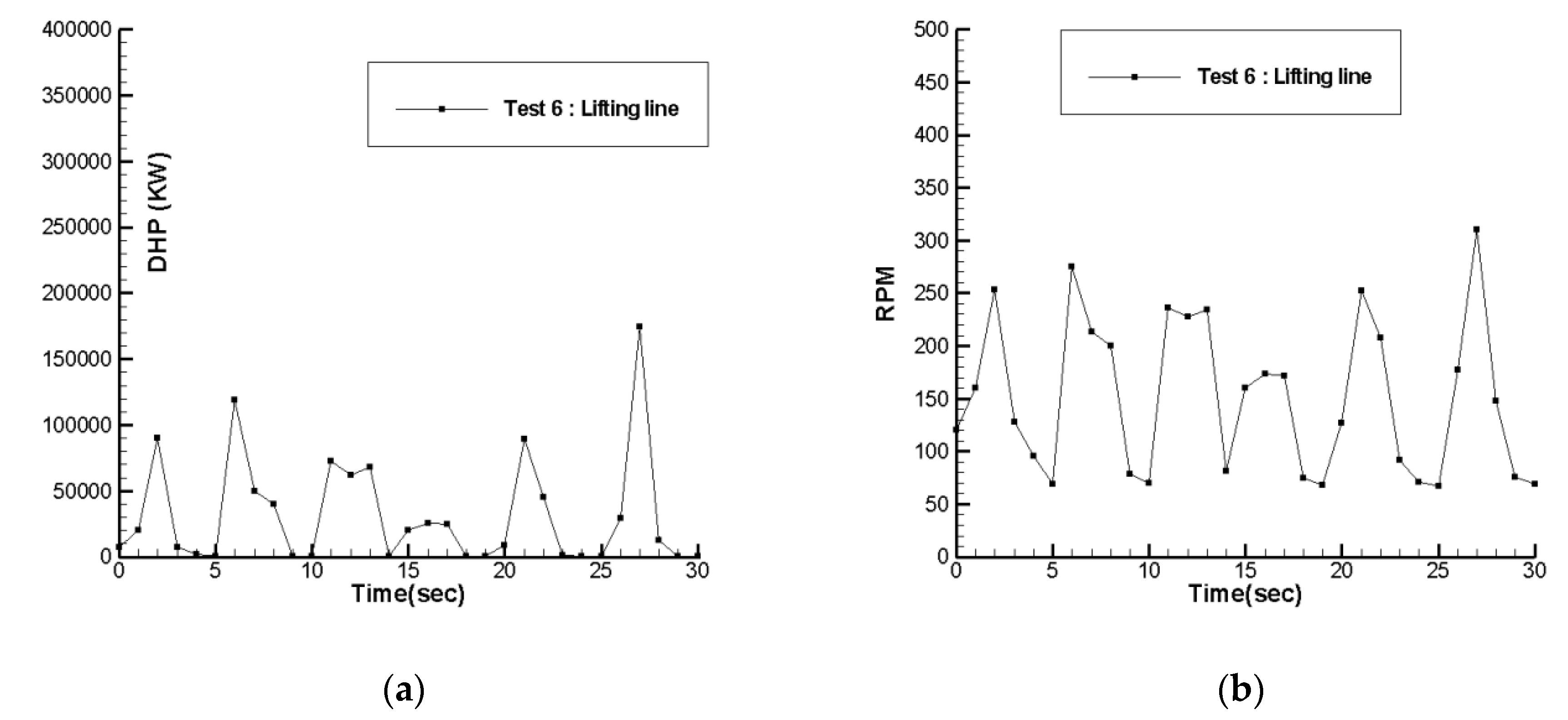
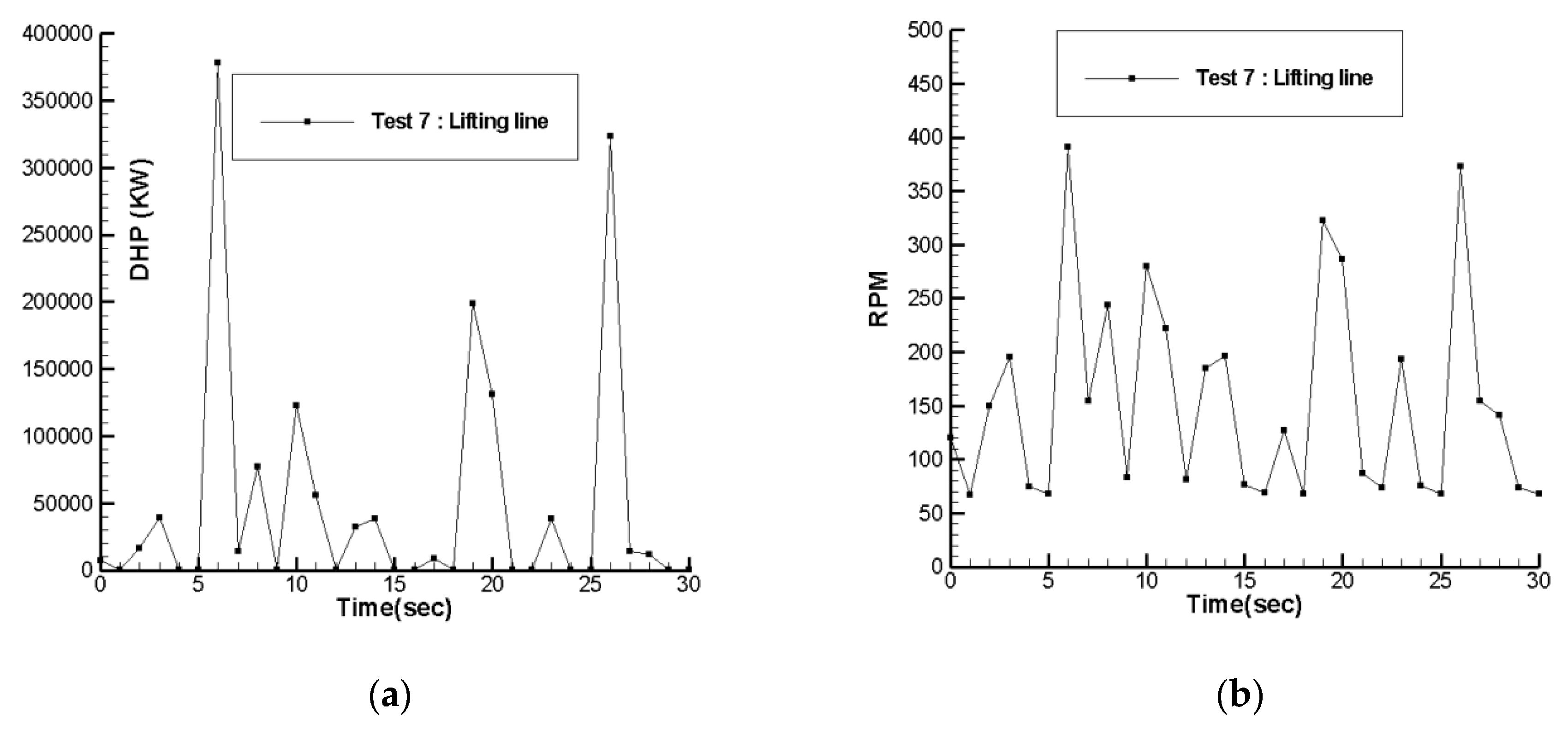
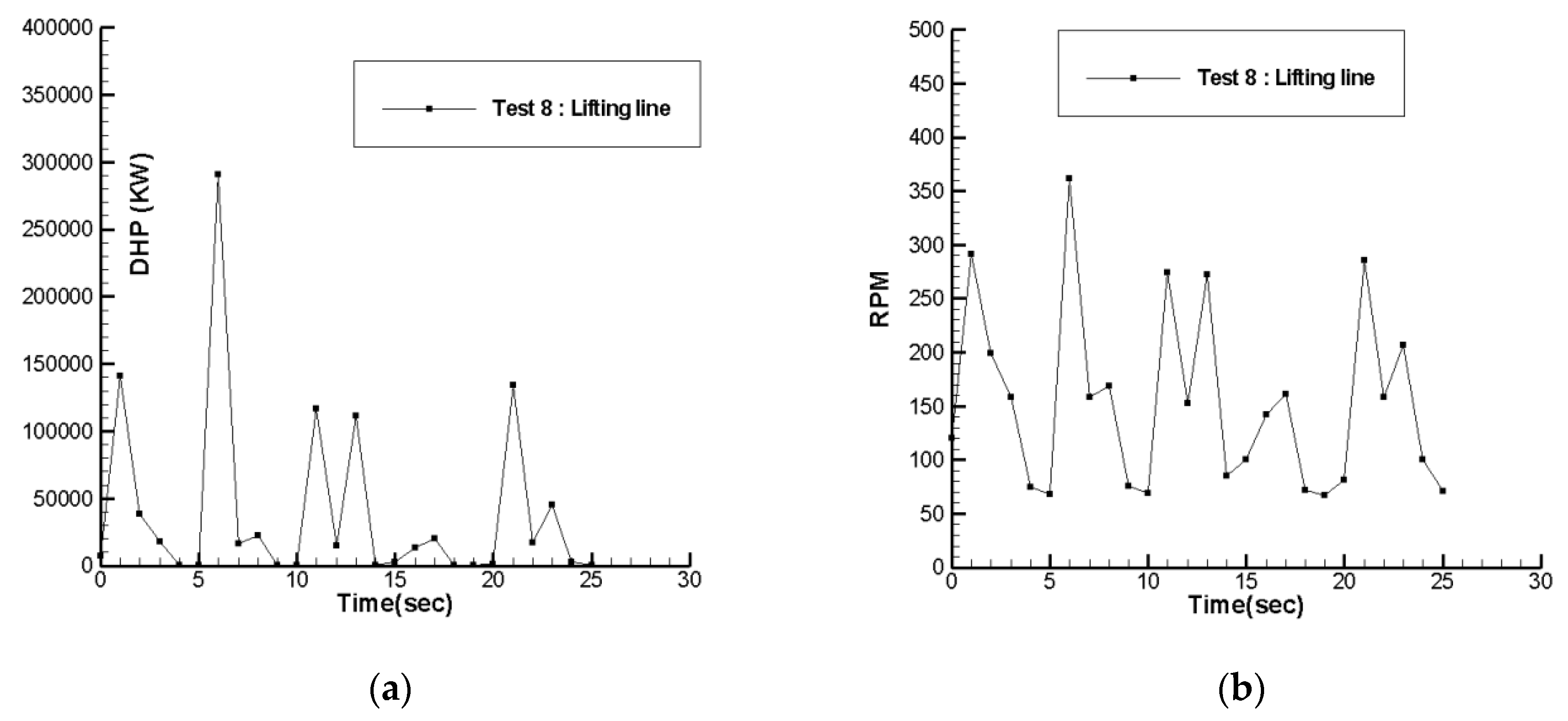
The results of the lifting line code concerning the propeller DHP and RPM are plotted on Figure 28, Figure 29, Figure 30, Figure 31, Figure 32, Figure 33, Figure 34 and Figure 35 for numerical experiments #1–#8. As observed, a quite unrealistic behavior is observed for DHP, exhibiting prohibitive high values at the positive peaks of C_T. The same conclusion holds for RPM which presents peaks of about 300% as regards the steady case. It should be taken into account that this behavior represents the propeller demands, whereas it is impossible for the engine to respond, because it has not the necessary margin and, besides, it cannot follow the extremely sudden peaks. Therefore, sustaining a constant speed seems to be an impossible situation, rendering the corresponding towing tank experiments questionable unless approximate estimations are made.

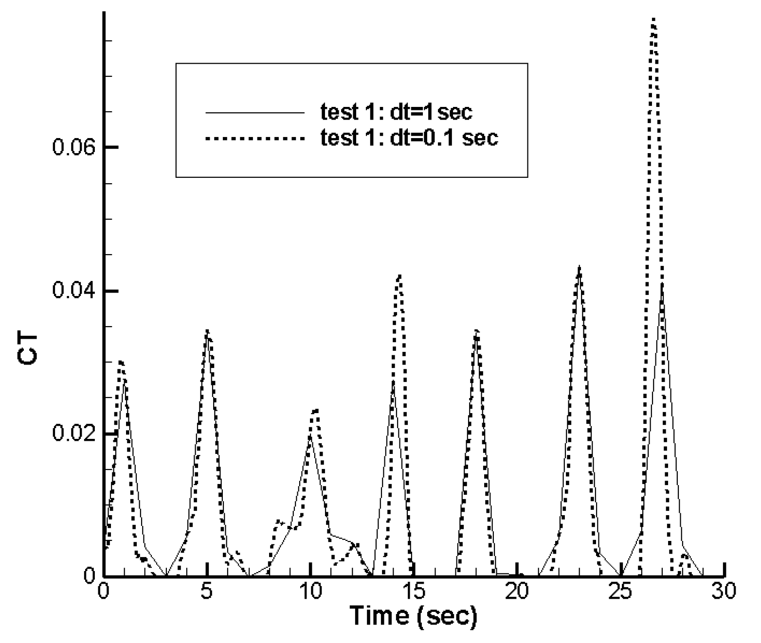
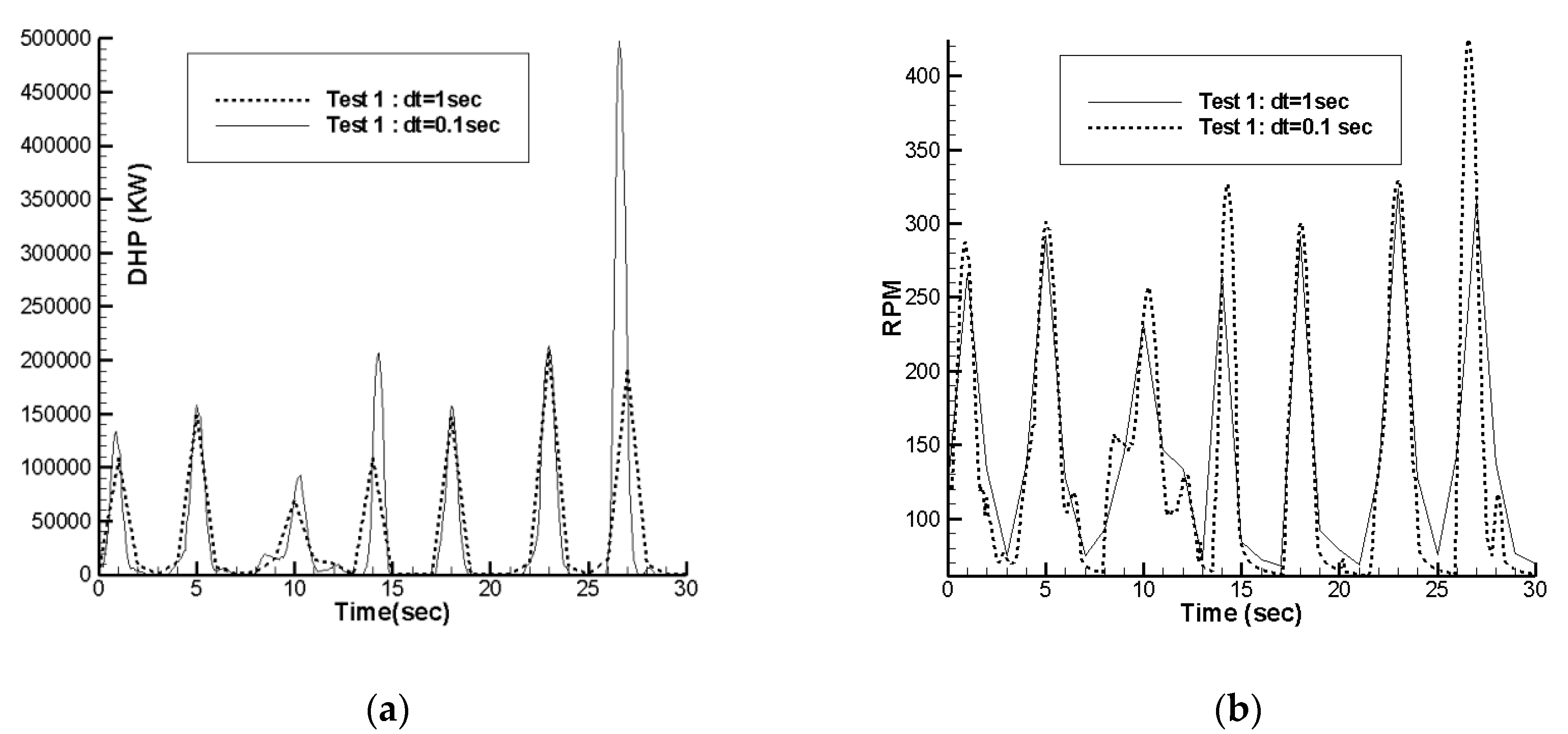
In order to investigate the effect of the selected time step, the numerical experiment #1 was repeated using a time step of 0.1 s. In Figure 36, the time histories of the thrust coefficient C_T are plotted for the Δt = 1 s and the Δt = 0.1 s tests. It is obvious that by using the lower value of Δt some peaks of the C_W,AD can be captured that have a direct influence on the total resistance coefficient. This is clearly shown around t = 15 s and t = 25 s. It is noticeable that the existence of such peaks in C_T do not affect the rest of the time history. As a direct consequence of this C_T behavior, the calculated values for the required DHP and propeller RPM are influenced accordingly, as shown in Figure 37. However, the observed differences due to Δt do not essentially change the basic conclusions concerning the prohibitive values of DHP and RPM.

Finally, it is interesting to study the self-propulsion of the ship at steady conditions, regarding the mean added wave resistance as an additional load on the propeller thrust. According to the experimental data, the mean added wave resistance component is calculated equal to 1.764 × 10^-3 and the corresponding propulsive characteristics are presented in

Table 11. Calculated propulsive characteristics at ship scale.

CT × 103	CF × 103	CP × 103	1-t	1-wn	1-we	DHP (kW)	RPM
5.736	1.518	2.481	0.542	0.669	12947	141.72	5.736

. Comparing the results with those of Table 9 for the calm water predictions, we can find an average increase of about 77% in DHP and 17.5% in RPM. These differences are still substantially higher than the usual margins of the ship’s engine, implying that there will be an actual loss of speed at the examined sea state.

4. Conclusions

A simplified numerical method has been employed for calculating the propulsion characteristics of a bulk-carrier in waves. Under the assumption that the ship moves at steady forward speed, the added resistance in time is estimated through the towing tank experiments and the propeller thrust is adjusted accordingly, while propeller action is modeled according to the actuator disk approach.

At first, computations were performed at model scale in still water in order to validate the method. Then, similar computations at full scale were conducted in order to calculate the ship’s resistance which was the basis for determining the added resistance in waves and the required propeller thrust.

Then, unsteady RANS computations were applied at a random sea state characterized by a prescribed power spectrum. In order to study the variation of propulsive parameters (including DHP and RPM) in time, it was assumed that the ship moved steadily and, besides, the propeller performance could be approximated by a quasi-steady procedure. The estimation of these parameters in a certain time period indicated that the propeller demands vary in an unrealistic way as regards the engine response. This behavior is rather due to the abrupt changes of the wave resistance which impose extremely high loads on the propeller. Therefore, the basic assumption of the steady forward speed in waves is subject to criticism.

Another crucial issue, related to the aforementioned study, is that the towing tank experiments in random waves at constant speed appear questionable as regards the self-propulsion behavior of a real ship. However, they are very useful to estimate the mead added resistance and, consequently, to predict the mean propulsion demands in a seaway. Such a numerical experiment was also performed in order to compute approximately the required engine margins for the examined bulk carrier.

References

- Chuang, Z.; Steen, S. Prediction of Speed Loss of a Ship in Waves; smp’11, Second International Symposium on Marine Propulsors: Hamburg, Germany, 2011. [Google Scholar]
- Tzabiras, G.D.; Polyzos, S.P. A hybrid numerical method for calculating self-propulsion characteristics of ships. In Proceedings of the IMAM 2015 International Conference, Pula, Croatia, 21–24 September 2015; pp. 51–58. [Google Scholar]
- Islam, H.; Rahaman, M.; Akimoto, H. Added Resistance Prediction of KVLCC2 in Oblique Waves. Am. J. Fluid Dyn. 2019, 9, 13–26. [Google Scholar]
- Taskara, B.; Yuma, K.; Steena, S.; Pedersen, E. The effect of waves on engine-propeller dynamics and propulsion performance of ships. Ocean. Eng. 2016, 122, 262–277. [Google Scholar] [CrossRef] [Green Version]
- Winden, B.; Badoe, C.; Turnock, S.; Phillips, A.; Hudson, D. Self propulsion in waves using a coupled RANS-BEMt model and active RPM control. In Proceedings of the NuTTS 13 16th Numerical Towing Tank Symposium, Duisburg, Germany, 2–4 September 2013. [Google Scholar]
- Wockner-Kluwe, K. Evaluation of the Unsteady Propeller Performance behind Ships in Waves. Ph.D. Thesis, Technical University of Hamburg, Hamburg, Germany, 2013. [Google Scholar]
- Sigmund, S.; el Moctar, O. Numerical Prediction of the Propulsion Characteristics of Ships in Waves. In Proceedings of the ASME 2016 35th International Conference on Ocean, Offshore and Arctic Engineering, Busan, Korea, 19–24 June 2016. [Google Scholar]
- Wang, J.; Wan, D. Computations of self-propulsion in waves of fully appended ONR Tumblehome model. In Proceedings of the ACFD11 The Eleven Asian Computational Fluid Dynamics Conference, Dalian, China, 16–20 September 2016. [Google Scholar]
- Peng, G.; Gao, Y.; Wen-hua, W.; Lin, L.; Huang, Y. Numerical Method to Simulate Self-Propulsion of Aframax Tanker in Irregular Waves. Math. Probl. Eng. 2020. [Google Scholar] [CrossRef]
- Tzabiras, G.D.; Kontogiannis, K. An integrated method for predicting the hydrodynamic performance of low cB ships. Comput. Aided Des. J. 2010, 42, 985–1000. [Google Scholar] [CrossRef]
- Menter, F. Zonal two equation turbulence models for aerodynamic flows. In Proceedings of the 24th Fluid Dynamics Conference, AIAA, Orlando, FL, USA, 6–9 July 1993. [Google Scholar]
- Van Leer, B. Towards the Ultimate Conservative Difference Scheme V, A second-order Sequel to Gudunov’s method. J. Comp. Phys 1979, 32, 101–136. [Google Scholar] [CrossRef]
- Roe, P.L. Some Contributions to the Modelling of Discontinuous Flows. In Lectures in Applied Mechanics; Springer: Berlin, Germany, 1985; Volume 22, pp. 163–193. [Google Scholar]
- Tzabiras, G.; Psaras, K. Numerical simulation of self-propulsion tests of a Product-carrier at Various conditions. In Proceedings of the HIPER-14 International Conference, Athens, Greece, 3–5 December 2014; pp. 92–102. [Google Scholar]
- Tzabiras, G.D. Resistance and self-propulsion simulations for a Series-60, cB = 0.6 hull at model and full scale. Ship Technol. Res. 2004, 51, 21–34. [Google Scholar] [CrossRef]
- Tzabiras, G.D. A numerical study of actuator disk parameters affecting the self-propulsion of a bulk-carrier. Int. Shipbuild. Prog. 1996, 1, 47–55. [Google Scholar]
- Tzabiras, G.D. A numerical study of additive bulb effects on the resistance and propulsion characteristics of a full ship form. Ship Technol. Res. 1997, 44, 98–108. [Google Scholar]
- Politis, G.K. A lifting line equivalent profile method for propeller calculation. J. Ship Res. 1985, 29, 241–251. [Google Scholar]
- Liarokapis, D.; Tsami, I.; Trahanas, J.; Tzabiras, G. An experimental study of the added resistance of a Bulk-carrier model. In Proceedings of the IMAM-2015 International Conference, Pula, Croatia, 21–24 September 2015; pp. 121–126. [Google Scholar]
- Tsami, I. Added Resistance Experiments on Ship Models. Diploma Thesis, National Technical university of Athens, Athens, Greece, 2013. (In Greek). [Google Scholar]
- Kiosidou, E.; Liarokapis, D.; Tzabiras, G.; Pantelis, D. Experimental investigation of roughness effect on ship resistance using flat plate and model towing tests. J. Ship Res. 2017, 61, 75–90. [Google Scholar] [CrossRef]
- ITTC. Recommended Procedures and Guidelines, Testing and Extrapolation Methods, Loads and Responses, Sea Keeping, Sea Keeping Experiments; 7.5-02-07-02.1; ITTC: Zürich, Switzerland, 2005. [Google Scholar]
- McHale, M.; Friendman, J. Standard for Verification and Validation in Computational Fluid Dynamics and Heat Transfer; ASME V&V the American Society of Mechanical Engineers: New York, NY, USA, 2009; Volume 20. [Google Scholar]
Figure 1.
The body-fitted block mesh around the hull.
Figure 2.
The hull shape.
Figure 3.
Scale model of the bulk-carrier in the towing tank of LSMH-NTUA.
Figure 4.
Water elevation η time series for Experiment #1.
Figure 5.
Water elevation η time series for Experiment #2.
Figure 6.
Water elevation η time series for Experiment #3.
Figure 7.
Water elevation η time series for Experiment #4.
Figure 8.
Water elevation η time series for Experiment #5.
Figure 9.
Water elevation η time series for Experiment #6.
Figure 10.
Water elevation η time series for Experiment #7.
Figure 11.
Water elevation η time series for Experiment #8.
Figure 12.
Power Density Spectrum, Bretschneider vs. Measured.
Figure 13.
Resistance time series for Experiment #1.
Figure 14.
Resistance time series for Experiment #2.
Figure 15.
Resistance time series for Experiment #3.
Figure 16.
Resistance time series for Experiment #4.
Figure 17.
Resistance time series for Experiment #5.
Figure 18.
Resistance time series for Experiment #6.
Figure 19.
Resistance time series for Experiment #7.
Figure 20.
Resistance time series for Experiment #8.
Figure 21.
Water elevation contours, model scale, Fn = 0.180.
Figure 22.
Water elevation around the bow (a) and the stern (b), model scale, Fn = 0.180.
Figure 23.
Axial velocity isowake curves on the propeller plane; on the left is the double body case and on the right the ship in calm water, for (a) the towed ship and (b) the self-propelled ship.
Figure 24.
Time histories of the thrust CT(t) and added wave resistance CW(t) coefficients, numerical experiment #1.
Figure 25.
Time histories of real (1-wd) and effective (1-we) wake fractions, numerical experiment #1.
Figure 26.
Axial velocity isowake curves on the propeller plane for a local maximum of the added resistance.
Figure 27.
Axial velocity isowake curves on the propeller plane for a local minimum of the added resistance.
Figure 28.
Time history of the required DHP (a) and RPM (b), numerical experiment #1.
Figure 29.
Time history of the required DHP (a) and RPM (b), numerical experiment #2.
Figure 30.
Time history of the required DHP (a) and RPM (b), numerical experiment #3.
Figure 31.
Time history of the required DHP (a) and RPM (b), numerical experiment #4.
Figure 32.
Time history of the required DHP (a) and RPM (b), numerical experiment #5.
Figure 33.
Time history of the required DHP (a) and RPM (b), numerical experiment #6.
Figure 34.
Time history of the required DHP (a) and RPM (b), numerical experiment #7.
Figure 35.
Time history of the required DHP (a) and RPM (b), numerical experiment #8.
Figure 36.
Comparison of the time history of the thrust (CT) coefficient, numerical experiment #1.
Figure 37.
Comparison of the time history of the required DHP (a) and RPM (b), numerical experiment #1.