Article

Appraisal of Climate Change and Its Impact on Water Resources of Pakistan: A Case Study of Mangla Watershed

1
Department of Irrigation and Drainage, University of Agriculture, Faisalabad 38000, Pakistan
2
Institute of International Rivers and Eco-Security, Yunan University, Kunming 650021, China
3
Department of Agricultural Engineering, Muhammad Nawaz Shareef University of Agriculture, Multan 66000, Pakistan
4
Department of Geoecology, Institute of Geosciences and Geography, University of Halle-Wittenberg, Von Seckendorff-Platz 4, 06120 Halle (Saale), Germany
5
Water Management Research Centre, University of Agriculture, Faisalabad 38000, Pakistan
6
Department of Land and Water Conservation Engineering, Faculty of Agricultural Engineering and Technology, PMAS-Arid Agriculture University, Rawalpindi 46000, Pakistan
7
Faculty of Agriculture and Environmental Sciences, University of Rostock, 18059 Rostock, Germany
*
Authors to whom correspondence should be addressed.
Atmosphere 2020, 11(10), 1071; https://doi.org/10.3390/atmos11101071
Submission received: 18 September 2020 / Revised: 6 October 2020 / Accepted: 7 October 2020 / Published: 9 October 2020
(This article belongs to the Special Issue Climates of the Himalayas: Present, Past and Future)

Abstract

:
Water resources are highly dependent on climatic variations. The quantification of climate change impacts on surface water availability is critical for agriculture production and flood management. The current study focuses on the projected streamflow variations in the transboundary Mangla Dam watershed. Precipitation and temperature changes combined with future water assessment in the watershed are projected by applying multiple downscaling techniques for three periods (2021–2039, 2040–2069, and 2070–2099). Streamflows are simulated by using the Soil and Water Assessment Tool (SWAT) for the outputs of five global circulation models (GCMs) and their ensembles under two representative concentration pathways (RCPs). Spatial and temporal changes in defined future flow indexes, such as base streamflow, average flow, and high streamflow have been investigated in this study. Results depicted an overall increase in average annual flows under RCP 4.5 and RCP 8.5 up until 2099. The maximum values of low flow, median flow, and high flows under RCP 4.5 were found to be 55.96 m3/s, 856.94 m3/s, and 7506.2 m3/s and under RCP 8.5, 63.29 m3/s, 945.26 m3/s, 7569.8 m3/s, respectively, for these ensembles GCMs till 2099. Under RCP 4.5, the maximum increases in maximum temperature (Tmax), minimum temperature (Tmin), precipitation (Pr), and average annual streamflow were estimated as 5.3 °C, 2.0 °C, 128.4%, and 155.52%, respectively, up until 2099. In the case of RCP 8.5, the maximum increase in these hydro-metrological variables was up to 8.9 °C, 8.2 °C, 180.3%, and 181.56%, respectively, up until 2099. The increases in Tmax, Tmin, and Pr using ensemble GCMs under RCP 4.5 were found to be 1.95 °C, 1.68 °C and 93.28% (2021–2039), 1.84 °C, 1.34 °C, and 75.88%(2040–2069), 1.57 °C, 1.27 °C and 72.7% (2070–2099), respectively. Under RCP 8.5, the projected increases in Tmax, Tmin, and Pr using ensemble GCMs were found as 2.26 °C, 2.23 °C and 78.65% (2021–2039), 2.73 °C, 2.53 °C, and 83.79% (2040–2069), 2.80 °C, 2.63 °C and 67.89% (2070–2099), respectively. Three seasons (spring, winter, and autumn) showed a remarkable increase in streamflow, while the summer season showed a decrease in inflows. Based on modeling results, it is expected that the Mangla Watershed will experience more frequent extreme flow events in the future, due to climate change. These results indicate that the study of climate change’s impact on the water resources under a suitable downscaling technique is imperative for proper planning and management of the water resources.

1. Introduction

Most of the countries in South Asia are observing water stress due to global atmospheric changes. The rising population in urban areas, agriculture, and mismanagement of water resources and climate change has included Pakistan in the countries that are worst affected by climate change [1]. According to a report by the International Monetary Fund (IMF), Pakistan positioned third in the world among the countries prone to severe water scarcity [2]. The International Panel for Climate Change (IPCC) reported a 0.72 °C increase in the total temperature from 1951 to 2012. An expected rise of 1 °C to 3 °C till 2050 and 2 °C to 5 °C is likely to occur until 2100, based on the different greenhouse gases emission scenario. The severe temperature changes affect the land cover and ultimately change the streamflow patterns [3]. Rivers are providing more than fifty percent of the global water requirement [4]. However, river flows are associated with long-term fluctuations in rainfall and temperature, especially in areas where snowmelt is the principal component of the total runoff [5,6].
General circulation models (GCMs) are widely in use to study future climate change drifts. These models simulate climate variations based on possible projected greenhouse gas emission rates. The spatial resolution of almost all existing GCM models is around 150–300 km, and the spatial resolution of every single GCM alters when comparing with other GCMs [7]. To accurately apprehend the impact of climate change on water resources, the bias correction of the projected results from different climatic models is often performed [8,9]. Bias correction is beneficial, especially for hydrological modeling studies where streamflow directly connects with precipitation [10,11,12]. GCMs present large-scale forecasts for several climatic variables [3], but numerous climatic variables are not determined efficiently through the coarser resolution. To overcome this issue, different downscaling techniques are often applied to downscale the projected GCMs data to a fine resolution, but these techniques also provide systematic deviations [13,14,15]. Many statistical downscaling techniques have been introduced to eliminate systematic deviations [16,17]. Specific downscaling procedures establish a connection between regional-scale climatic components with the local scale climatic components. By studying the transfer of moisture at a regional scale and air blowing rate, the temperature and precipitation at a local scale can be predicted [18,19,20,21]. In statistical downscaling techniques, the spatial resolution of the GCMs is not considered, so the calculation of bias correction coefficient must be done effectively by using long period observed and historical climatic data [22,23]. Multiple studies deal with the drifts of hydro-climatic components of various basins in the upper Indus basin, using several statistical downscaling techniques, and a continuous rise in temperature was projected [24,25,26,27]. Nevertheless, the temperature is progressing at varying rates in various sub-basins. The history explains numerous rainfall drifts in various sub-basins present in the upper Indus basin [28].
To understand the hydrologic processes and interaction of water balance components under climate change scenarios in Mangla Watershed, the Soil and Water Assessment Tool (SWAT) model is used in this study. SWAT is proficient in modeling a single catchment or a system of hydrologically connected sub-catchments. The GIS-based interface model, ArcSWAT, defines the river network and the point of catchment outflow, and the distribution of sub-catchments and hydrological response units (HRU) [12,29,30,31,32,33,34,35]. The calculation of the time of concentration by SWAT is done by adding overland flow time (time is taken for flow from the remotest point of the sub-basin to reach the water channel) and channel flow time (time taken from upstream channel to the watershed outlet) [36].
The projected climate is significantly affected by the selection of GCMs [35]. In this study, five global circulation models: The Australian Community Climate and Earth-System Simulator version 1 (ACCESS 1.0), Community Climate System Model (CCSM4), Hadley Centre Global Environment Model version 2 (HadGEM2), Max Planck Institute for Meteorology, Earth System Model Low Radiation Emission (MPI-ESM-LR), and Model for Interdisciplinary Research on Climate, Earth System Model (MirocESM), were selected based on their spatial resolution, and two different emission scenarios, RCP 4.5, and RCP 8.5 were chosen to reproduce future streamflow by applying the hydrological model SWAT (ArcSWAT-2012).
Several studies have defined precipitation and temperature variations as dominating factors that may affect water quantity and quality [37,38,39] and reported how climate change affects river flows [21,27,40]. Few studies have reported climate change effects on the average annual streamflow in the Mangla Watershed [32,41], however, the literature on the impact of future climate change on the annual and seasonal base flows and high flows in the watershed is missing. Moreover, investigation of the impact of future climate change on streamflow by considering the elevation band in watersheds is also missing. Previously, only biased corrections of the downscaled GCMs data had been performed without studying the different downscaling techniques. The current study has also used multiple downscaling techniques for projecting future water resources in the study area. The main objectives of this study are (i) the development of a hydrological model for the transboundary Mangla Dam watershed with the use of daily precipitation, temperature, and streamflow data (ii) future projection of precipitation and temperature from GCM data using three statistical downscaling techniques and their comparison, (iii) estimation of future climate change impacts on the transboundary Mangla Dam basin’s streamflow. This study could be helpful to the water resource managers for the better administration of water resources, by modifying the management plans to mitigate the effects of climate change in the future.

2. Material and Methods
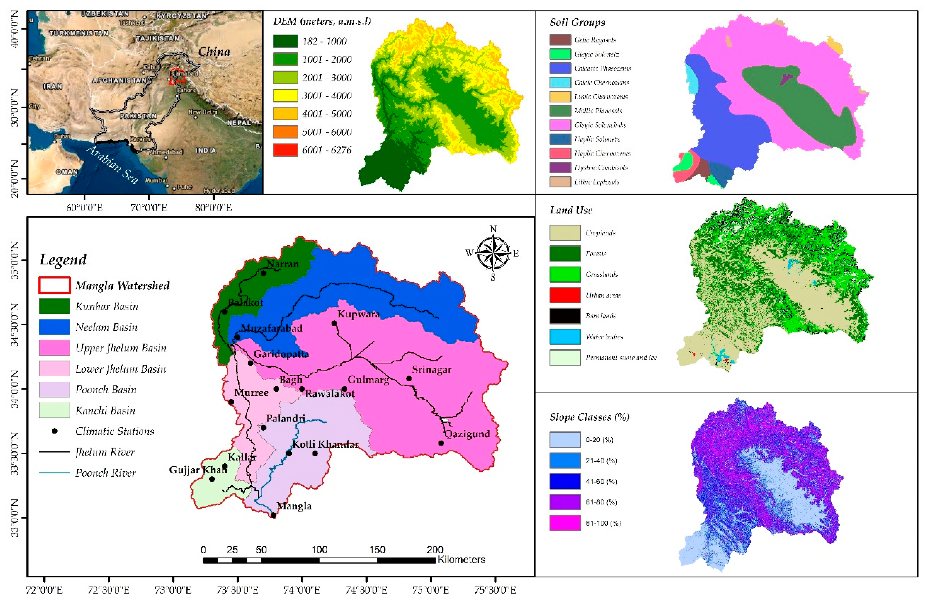
2.1. Study Area

The transboundary Mangla Watershed ranges from 73°55’ to 75°35’ east of longitude and 33°25’ to 34°40’ north of latitude and is situated in the northeastern part of Pakistan and western part of the Himalaya. The geographical location of the watershed and considered weather station along with the land use and soil types in the watershed are presented in Figure 1. The Jhelum River is a main tributary of the Indus River and the Mangla Dam is built on this River. The maximum elevation in the Mangla watershed is about 5840 m, whereas the minimum elevation is 182 m above the mean sea level (a.m.s.l.). The total area of Mangla watershed is about 33,490 km2. Immense icecaps are present in the watershed, which provides large water volume to the Jhelum River by melting the ice, which eventually contributes to the Mangla Dam reservoir. The Mangla Dam was constructed in 1967 with an accommodation limit of 6.5 billion cubic meters of water. Almost 56% of the rear of the Mangla Watershed belongs to the Jhelum River, while 12% belongs to Poonch River, as shown in Figure 1. The total inflows into the Mangla dam are 1699.01 m3/s, whereas outflows are 566.34 m3/s. The hydro-power generation capacity of the Mangla dam is about 1310 MW. The mean population density in the watershed varies from 350 to 1000 people per square kilometer in the mountainous and cultivated regions, respectively. The average Tmax of Mangla Watershed ranges between 10.6–31.6 °C, and the average minimum temperature ranges from 4–25 °C. Soil data were downloaded from the website [42] land use data, and DEM data were downloaded from [43,44].

2.2. Data Collection

2.2.1. Climate Data

Daily observed data of climate variables such as Tmax, Tmin, and precipitation were obtained from the statistics files of the Pakistan Meteorological Department (PMD) and Water and Power Development Authority (WAPDA). Daily rainfall data for years 1981–2010 were provided by Pakistan Meteorology Department to quantify the outflow of the basin. Figure 2 shows the average annual temperature trends from 1981 to 2010 at Mangla Watershed. The maximum temperature increased at a rate of 0.373 °C per decade (Figure 2a), and the rate of rising of minimum temperature was observed as 0.139 °C per decade (Figure 2b).

2.2.2. Global Climatic Models (GCMs) Data

In this study, five global circulation models; ACCESS, CCSM4, HadGEM2, ESMLR, and MirocESM were selected based on their spatial resolution [45]. Two representative concentration pathways (RCPs), RCP 4.5, and RCP 8.5 were considered for these five GCMs. The data were downloaded from [46]. The details about these GCMs can be found from the user guide of CMIP5 [7].

2.2.3. Landuse and Soil Data

The soil data were downloaded from the Food and Agriculture Organization (FAO) website [42]. The downloaded harmonized soil 30 arc-second raster database covers the entire globe and displays the composition and characterization of different soil parameters, such as soil texture, ion exchange capacity, water holding capacity, soil depth, soil pH, soil temperature, lime and gypsum contents, granulometry, etc. The information about land use land cover (LULC) was downloaded from the United States Geological Survey (USGS) website [44]. The land-use data is a raster dataset, with a fine spatial resolution of 30 m by 30 m and covers a detailed 27 land cover and vegetation classification. The land use data provide detailed information about several types of agricultural lands, forests, vegetation, and grasslands present in any specific part of the globe. They also provide details about the snow-covered area, water bodies, artificial or urban areas, and barren lands. The hydrological model SWAT was parameterized using remotely sensed satellite datasets on soil, land cover, and topography. Based on the USGS soil classification system, the Mangla watershed have more than 45 percent of agricultural lands. Table 1 revealed that the most prominent land-use existing in the watershed is croplands, either artificially or irrigated covering, almost 45.38 percent of the area. The second widely spread class is grasslands, or green lands covered by needle leaves plants and covers 18.85 percent of the watershed area. The permanent snow-covered region covers approximately 3.91 percent of the Mangla watershed. Almost 1300 km2 of the watershed is under permanent ice-caps and snow reserves.
Details of soil data are presented in Table 2. The most prominent soil type in the watershed is loamy soil, which covered up to 71.04% of Mangla Watershed. The second classification represents the clayey soil, covers 24% of the total area, and other soils or water reservoirs surround the remaining 5% of the entire area. The GleyicSolonchak soil under group C holds 47.08% area of the watershed. Soil group C denotes those soils having low infiltration speeds when they remain fully saturated and uniform, with textures from medium-fine to moderately thick. These soils allow a reasonable water transportation rate. The principal soil collection comprises the Gleyic Solonchak group, which includes almost 47.087% of the watershed. The other groups hold Calcaric Phaeozems that cover about 23.429% of the area. The Mollic Planosols, Haplic Chernozems, Haplic Solonetz, Calcic Chernozems, Gelic Regosols, Luvic Chernozems, Lithic Leptosols, and Dystric Cambisols occupy 20.694%, 1.889%, 1.616%, 1.491%, 1.163%, 1.162%, 0.702%, 0.418%, and 0.342% of the total area of the watershed. Soil characteristics such as soil texture, soil bulk density, soil composition, soil electric conductivity, and soil possible water retention were collected from the FAO website. Wetland forests (WETF) are tree type crops [47]. The SWAT model has a built-in function to handle WETF by using several crop parameters, such as the ratio of erosion from land cropped to the clean tilled fallow continuous (USLE C factor), temperature responses, leaf area development, energy biomass conversion, light interception, stomatal conductance, canopy height, and root depth, plant nutrient content, and harvest. Detailed information on these parameters is given in [47].
SWAT model uses the value of soil available water contents (AWC) in mm/mm. The values of AWC were used in mm/mm during the model run. The values of AWC added in the user soil table, located in the SWAT_2012 database, were 0.064 for Gelic Regosols, 0.071 for Gleyic Solonetz, 0.170 for Calcaric Phaeozems, 0.081 for Calcic Chernozems, 0.048 for Luvic Chernozems, 0.090 for Mollic Planosols, 0.175 for Gleyic Solonchaks, 0.078 for Haplic Solonetz, 0.175 for Haplic Chernozems, 0.175 Lithic Leptosols and 0.175 for Dystric Cambisols.

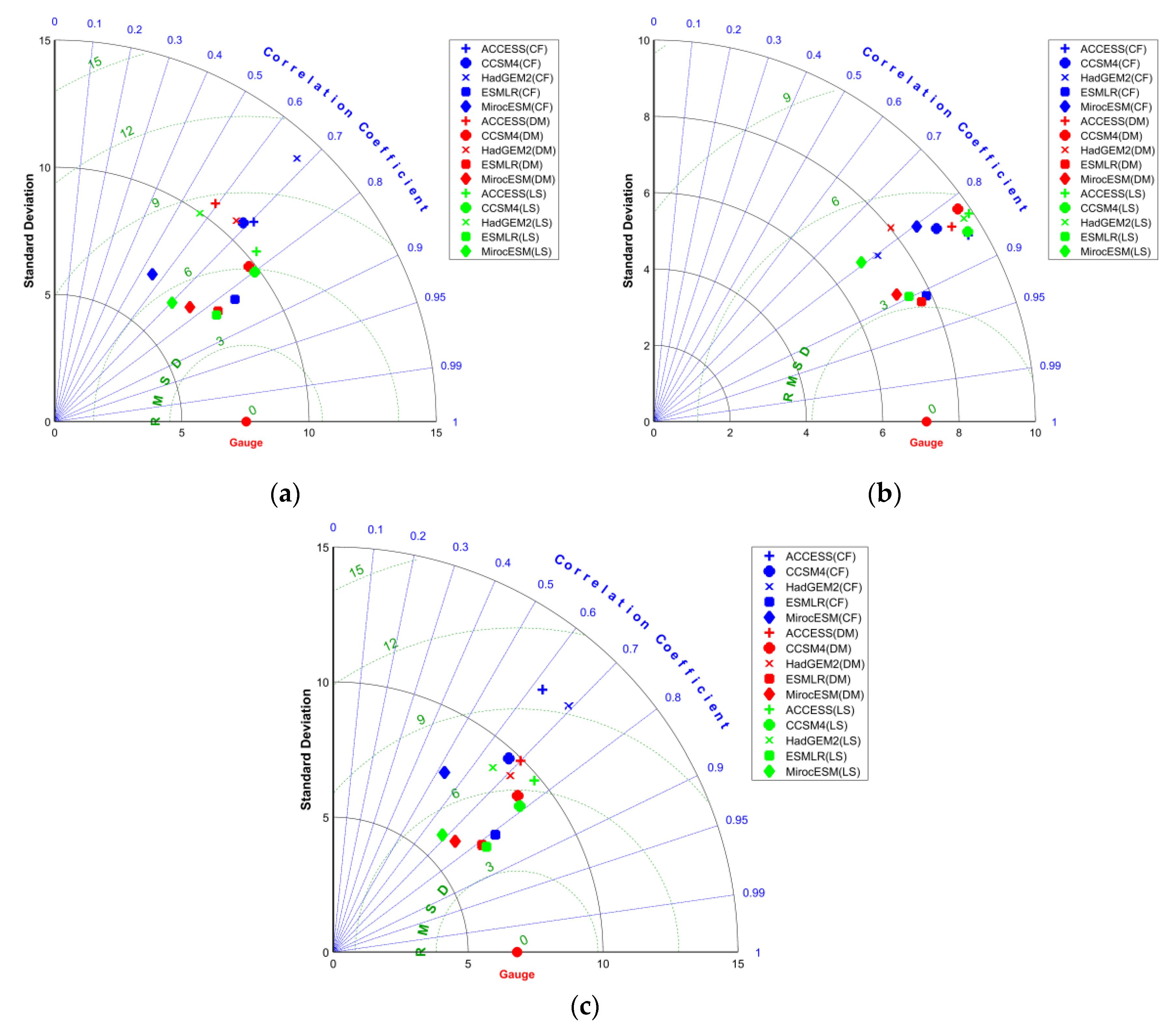
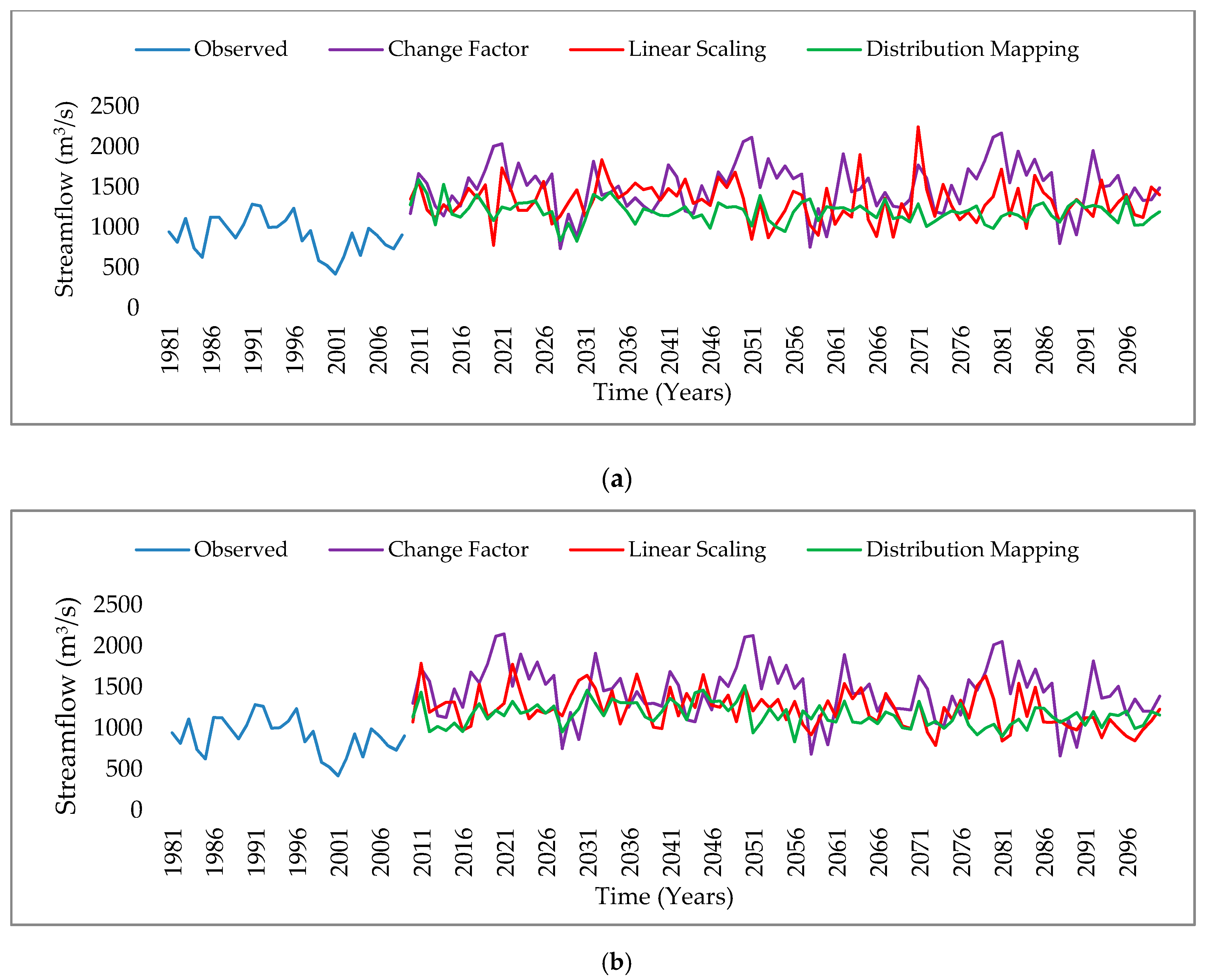
2.3. Statistical Downscaling

The large-scale gridded GCMs data were downscaled to predict the climatic conditions at a local scale. Statistical downscaling can be performed by setting mathematical relations between large-scale GCMs climatic variables and the local climatic variable. Statistical downscaling is much easy to interpret than dynamical downscaling. However, statistical downscaling depends massively on historical climatic data and gauged data. In this study, three different types of downscaling techniques were used.
  • Change factor (additive for temperature and multiplicative for precipitation)
  • Linear scaling (additive for temperature and multiplicative for precipitation)
  • Distribution mapping (additive for temperature and multiplicative for precipitation)
In change factor downscaling, the bias correction for the temperature (maximum and minimum) was done by adding the difference of monthly changes among the future and base years GCM in the observed temperature data. The bias correction coefficient was calculated for precipitation by dividing the monthly mean of GCM future precipitation data by GCM baseline precipitation data. The calculated bias correction coefficient was multiplied by observed precipitation data to obtain the modified/adjusted/bias-corrected precipitation [48]. The bias correction coefficient for precipitation in linear scaling downscaling was calculated by dividing long term monthly mean of gauged precipitation data with that of mean monthly GCMs, then this bias correction coefficient was multiplied with daily GCMs raw data to get corrected GCMs data [49]. Similarly, for the time-series data of temperature, an additive quotient was calculated by subtracting the long-term monthly mean of the GCMs simulated data from the long term monthly mean of observed data. The calculated bias correction coefficient was added in the daily GCMs raw data to obtain corrected GCMs data [49]. Distribution mapping (DM) is a commonly used bias-correction technique employed in various climate change studies [12,33,34,50]. Its basic working principle is to reproduce a transfer function based on the monthly mean value of GCMs data to the gauged data. The Gamma transfer function and Gaussian transfer function for precipitation and temperature data need to be reproduced, respectively, for correcting the bias from the downscaled future GCMs data [49].
Table 3 describes the five selected global climatic models used in this study. The GCMs were selected based on their spatial resolution. The projected climatic parameters vary extensively for different GCMs [35] and multiple GCMs are recommended for future projections, as single GCMs may cause uncertainty in the projected results. The data from five GCMs were downscaled by using three downscaling techniques, change factor downscaling, linear scaling downscaling, and distribution mapping downscaling. To investigate the suitability of the downscaling techniques, the downscaled data from all three downscaling techniques were compared with observed data using different statistical parameters, such as standard deviation and correlation coefficient. Figure 3 explains that there is a strong correlation between all three downscaling techniques and gauge data, i.e., above 0.56. In the case of the distribution mapping downscaling technique, the results were better than linear scaling and change factor downscaling techniques; the correlation of distribution mapping downscaling with observed data is above 90% for the GCM ESMLR in case of minimum temperature. Based on the correlation coefficient, standard deviation and root mean square deviation, as shown in Figure 3, it was concluded that the GCMs, ESMLR, and MirocESM has a maximum value of correlation coefficient (CC) as 0.83 and 0.80 respectively and minimum value of root mean square deviation (RMSD) 4.41 and 4.61 respectively for Tmax. ESMLR and MirocESM also have a maximum value of CC as 0.91 and 0.89 and a minimum value of RMSD as 3.14 and 3.42 respectively for Tmin. After the analysis of precipitation data, the CC of ESMLR and MirocESM also resulted in maximum reading as 0.81 and 0.74 under the distribution mapping downscaling technique. The GCMs, MirocESM, and ESMLR were found to be more accurate than other GCMs, and distribution mapping downscaling was found to be a more suitable downscaling technique for the transboundary of Mangla watershed to study climatic parameters such as maximum and minimum temperature and precipitation. The linear scaling downscaling technique is found to be less accurate than change factor downscaling [51]. The findings of this research consistent with previous studies such as [51] predicted that linear scaling is less suitable than change factor, whereas [52] studied that the distribution mapping performed better than other downscaling techniques. CMHyd software was used for linear scaling and distribution mapping, in which data were used directly in NetCDF files format [53]. Climate Model Data for Hydrologic Modeling (CMhyd) software was downloaded from the website of SWAT [54]. Using observed data of 30 years and historical data for 30 years, future data were downscaled. In CMhyd software, the overlapping of observed and historical data periods should be as long as 20 to 30 years [53]. If the overlapping period is less than 10 years, then results will not be considered appropriate. More details of the CMhyd software can be found in the user manual of CMhyd [53]. Change factor downscaling is showing some ambiguities and the correlation factor is less than 0.75 for model “ACCESS”. On the other hand, there is a strong correlation for model “ESMLR” i.e., more than 0.8 in all three downscaling techniques.

2.4. SWAT Model Description and Setup

The SWAT model [55], developed by the United States Department of Agriculture, is broadly being used for the assessment of the footprint of climate change in water resources studies. The main objectives of SWAT model development are to simulate the quality and quantity of surface and groundwater and to predict the environmental impact of land use, land management practices, and climate change [56]. Previously, numerous researchers utilized the SWAT model for hydrological modeling studies in the various basin and sub-basin scales [29,31,45,57,58,59,60,61].
The digital elevation model (DEM) is used for watershed delineation to investigate several properties of the basin, such as soil, slope, elevation, length of flow, streams created the longest path, etc. SWAT requires specific information on water abstraction that includes climate, land use, and land cover practices, topography, and river basin management to simulate hydrological processes. Similar properties within sub-basins can be combined into HRUs. The HRUs are spatially separated, and their replication results are added directly to the sub-basins for the entire basin path. In addition to the frequently used HRU discretization, the SWAT can also be discretized based on the groups or grids [56]. To perfectly reproduce the transfer of deposits, pesticides, and nutrients, the hydrological sequence, as prognosticated with the model, should define the historical trends of the basin. The detail about the model setup can be found in the user manual of ArcSWAT [60].

2.4.1. Slope Classification

Figure 1 and Table 4 provide the details of slope classes in the Mangla Watershed. Three slope classes were selected. The first-class ranges from 0 to 20%, the second class ranges from 21 to 40%, the third class ranges from 41 to 60%, fourth ranges from 61–80%, and fifth covers the slopes greater than 80%. First-class shows the minimum slope, while the fifth class slope represents the hilly areas having higher slopes or mountainous areas. The overall slope within the watershed is higher, and due to greater slopes, the accurate and precise specification of elevation is mandatory to effectively study the flow regimes within a partially or fully snow-covered watershed. In this study, to the precise specification of the elevation, the concept of elevation bands was employed.

2.4.2. Elevation Bands

The precise specification of alterations in elevation plays a crucial role in the hydrological modeling studies. Elevation bands play a significant role in the SWAT model for streamflow generation within a fully or partially snow-covered region, as the snow usually melts first at the lower elevation and later at a higher elevation. Similarly, for precipitation, it will fall as fresh snow at a higher altitude, and as rainfall on lower altitudes [62]. As a result of the interdependence of snow-fall and rainfall on elevation, the SWAT model simulations by considering the elevation bands will generate accurate results. The upper limit of the elevation bands is 10 in SWAT 2012, so in this study, ten elevation bands were incorporated to get the possible accuracy in results. The inter-comparison between the results obtained by consideration of elevation bands and without elevation bands was studied by [63] and interpreted that the results in fully or partially snow-covered watershed will not be accurate without considering elevation bands.

2.4.3. Model Accuracy Criteria

The performance of a model can be estimated by comparing the observed streamflow and model-simulated streamflow. There are several parameters to check the performance of the model such as coefficient of determination, the efficiency of Nash–Sutcliffe, and percentage bias. By looking at the observed and calibrated hydrographs, a researcher can recognize the adaptability of the model if the model is too fast or is underestimated. However, to quantitatively evaluate the performance of the model, numerical quantities related to the efficiency of the model are required.
Coefficient of determination (R2): The coefficient of determination R2 estimates the percentage of distinction in the observed data that is introduced in the results of the simulated model.
Efficiency coefficient Nash–Sutcliffe: The efficiency coefficient used by Nash–Sutcliffe to evaluate the future predictive strength of almost all hydrological models. The main limitation of the Nash–Sutcliffe efficiency includes the fact that the variations between the observed outflow and the simulated outflow values are determined by the squared values. This leads to an overestimation of the performance of the model through outflow peaks and an underestimation of the basic output flows. To check the model performance, the following parameters are considered:
(a)
The efficiency of Nash–Sutcliffe (NSE)
(b)
Bias percentage (Pbias)
(c)
Pearson’s coefficient for correlation (r)
(d)
Coefficient of determination R2
If the NSE value for calibration and validation is above 0.65, then the results are very good. However, if the NSE values fall below 0.5, then the results must not be considered satisfactory for the strong footing of the model [64,65,66,67]. If the PBIAS result of the model is less than 0.1, then the results are very good and increase in the values to 0.15. The results remain in an acceptable range, but when the values of PBIAS cross 0.25, then the result falls into an unsatisfactory range; calibration must be repeated by using different parameters along with a different parametric range [68,69]. If the Pearson correlation coefficient value is between 0.81 and 1, then the model performance will be very strong. If the performance confidence index is between 0.75 and 0.85, then the model performance will be very strong [67].

2.4.4. Model Calibration and Validation

SWAT model calibration was done using SWAT-CUP SUFI2 Algorithm for a period of 15 years, starting from January 1981 to December 1995. The objective function R2 was used during the calibration period. Three years were set-up as a warm-up period. The same parameters along with their values and the same number of iterations are further used to validate the model. The validation was done for a period of 15 years, from January 1995 to December 2010. Several parameters such as p-factor, r-factor, R2, NSE, PBIAS were calculated to check the performance of the SWAT model. P-factor represents the percentage of gauged data wrapped by the simulated 95% uncertainty band. R-factor represents the thickness of the 95% uncertainty band. The values of the p-factor should be greater than 0.70, whereas the values of the r-factor should be closer to zero. The range of p-factor is 0 to 1, whereas the range of r-factor lies between 0 and infinity [70].

3. Results

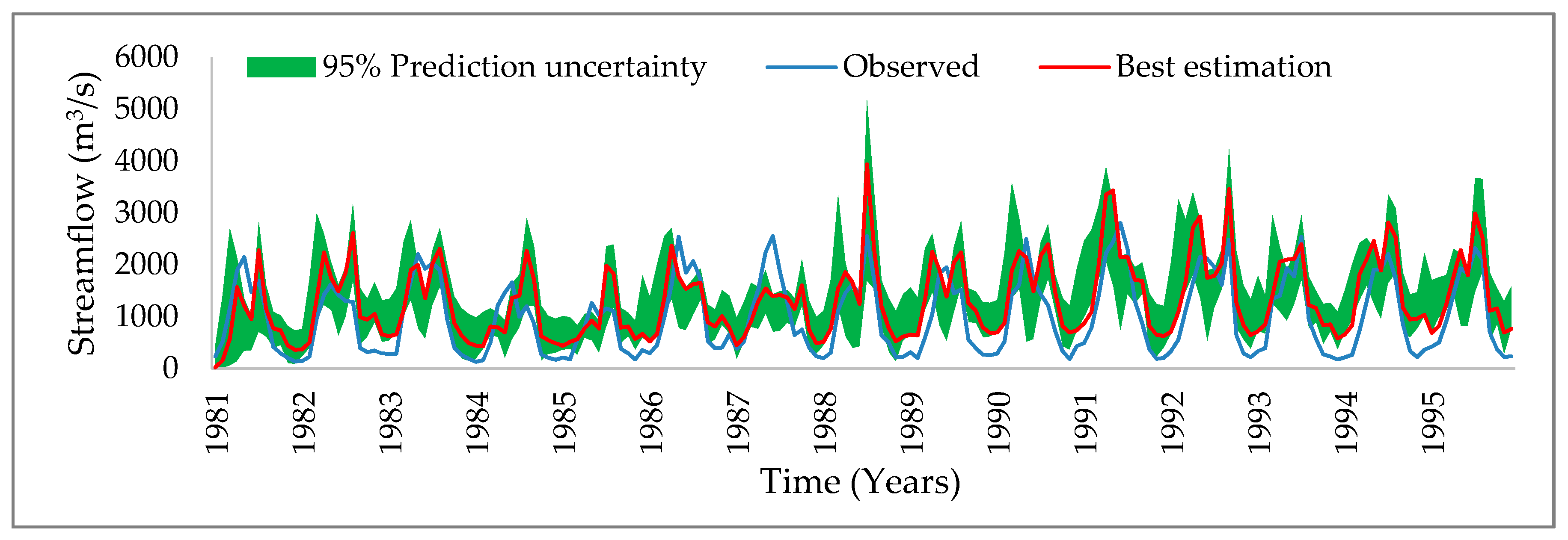
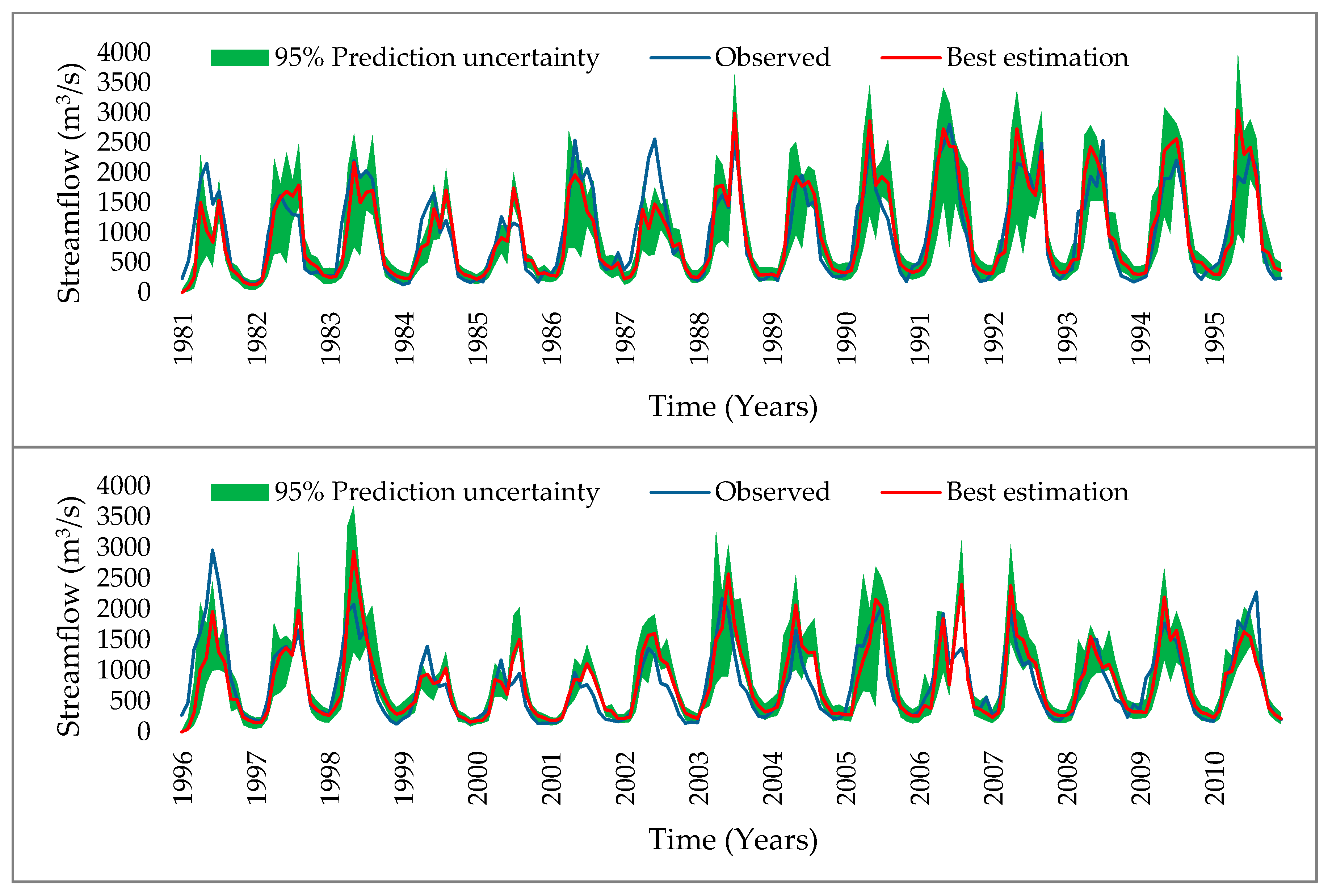
3.1. Model Calibration and Validation

3.1.1. Model Calibration without Considering Elevation Bands

The results of calibration and validation without considering elevation bands in Mangla watershed show a poor model performance, as represented in Figure 4. SWAT model calibration and validation performance evaluation indices, such as p-factor, r-factor, R2, NSE, and PBIAS, did not result in an acceptable range [67].
Figure 4 depicts the poor correlation between observed and simulated flows, as these results were simulated without considering elevation bands. The results of calibration without considering elevation bands for p-factor, r-factor, R2, NSE, and PBIAS were 0.43, 1.46, 0.68, 0.46, and −32. The results of the model performance indices, such as p-factor, r-factor, R2, NSE, and PBIAS, show the poor performance of the model in the Mangla Watershed without the use of elevation bands. So, in this research we recommend the hydrological modeling researchers to consider precise elevation bands to obtain accurate simulated results.

3.1.2. Calibration and Validation Considering Elevation Bands

Calibration and validation results revealed a strong model performance that can be potentially utilized to investigate the impacts of climate change on stream outflows (Figure 5). A strong relationship between model-simulated and observed flows was exhibited, which shows a strong footing of the SWAT model for future flow projections. The values for p-factor, r-factor, R2, NSE, PBIAS are 0.77, 0.99, 0.80, 0.78, and 1.1, respectively. These results show the strong footing of the model for future prediction. The R2 value is 0.80, which shows a strong relationship between the simulated and observed flow. Pbias should be between −20 to +20, and for perfect model footing, it should be close to zero. The pbias value for calibration is closer to the ideal, which is 1.1, which shows a great model performance for future projections. The NSE value in SWAT-CUP results is 0.78, which also represents the accuracy of model calibration.
The results of R2, NSE, pbias, p-factor, and r-factor, for calibration and validation, are presented in Table 5. These results depict that the SWAT model performance in the Mangla watershed is very strong [67].
The initial values of some parameters, such as curve number 2 for soil conservation services (CN2), the alpha factor for base flow in bank storage (days) (ALPHA_BF), delay in groundwater in days (GW_DELAY), the minimum depth of water in the shallow aquifer essential for backflow (mm) GWQMN, and groundwater revap coefficient (GW_REVAP), were taken from the literature [30]. The parameters used during the model calibration are shown in Table 6. The northern part of the Mangla Watershed is a partially snow-covered region [32] so some snow cover parameters, such as the temperature of snowfall (SFTM), the Base temperature of snowmelt (SMTMP), the maximum rate of snowmelt over a year (SMFMX), the minimum rate of snowmelt over a year (SMFMN), the minimum amount of snow water resembles 100% of snow cover (SNOCOVMX), and the volume of snow that corresponds to 50% of snow cover (SNO50COV), were also utilized. The minimum initial value given to SFTM is −5 and the maximum value given is 5. The parameter SNOCOVMX was initially set between 0 and 400, whereas the minimum and maximum values designated to SNO50COV were 0.1 and 0.6. More details about these parameters can be found in the user manual of SWAT-CUP_2012 [70].

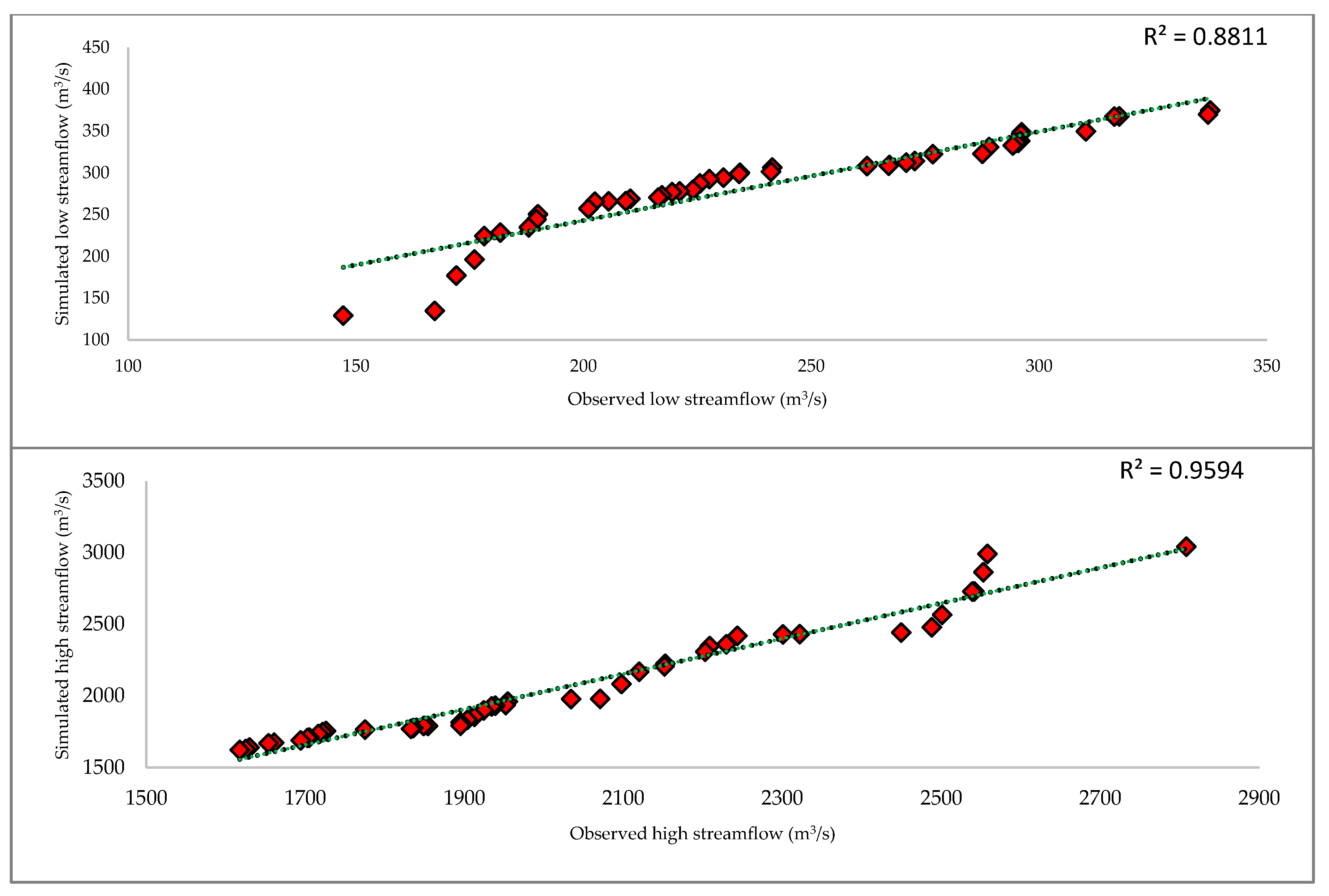
3.2. Performance Evaluation of The SWAT Model in Terms of Low and High Flows

The simulated low streamflow and high streamflow by the SWAT model were compared with observed low stream flows and observed high streamflow, respectively. The results indicated a strong correlation coefficient of 0.94 and 0.98 for low and high streamflow, respectively. The values of the coefficient of determination (R2) also indicated that the SWAT model performed well in simulating low and high streamflow. The R2 values were 0.88 and 0.96 for low streamflow and high streamflow respectively. Figure 6 shows the comparison between observed and simulated low streamflow and observed and simulated high streamflow. The values of the coefficient of determination (R2) also represent that the observed and simulated low flows and observed and simulated high flows have a strong relationship. These indices depict that the SWAT model is performing well in simulating low flows and high flows.

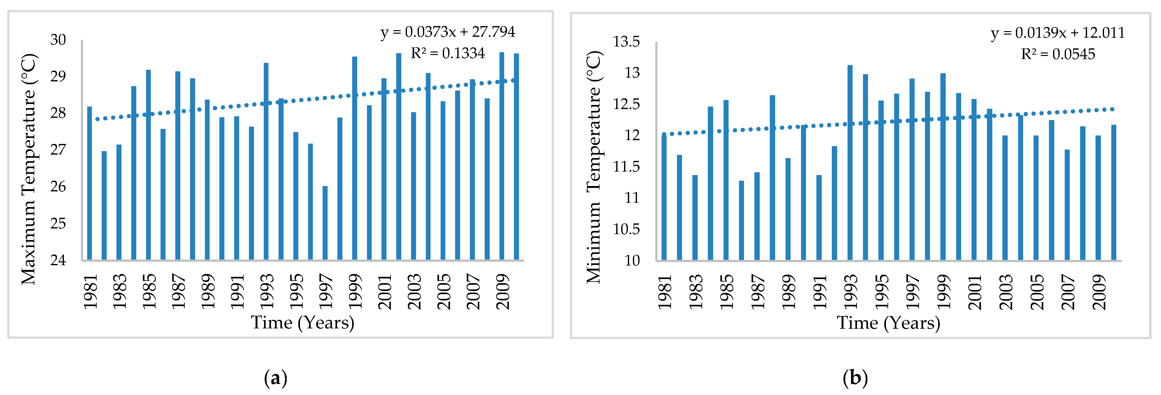
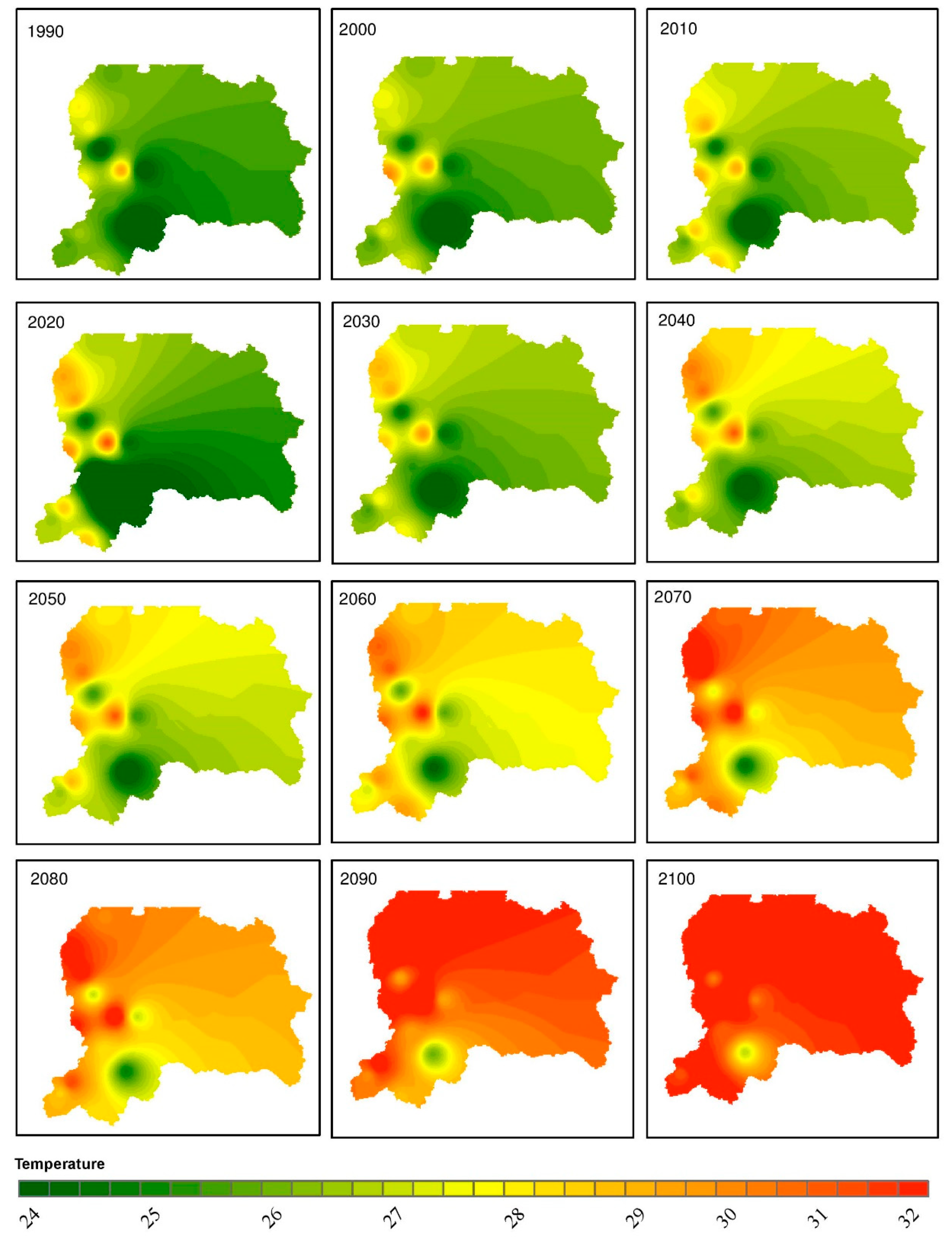
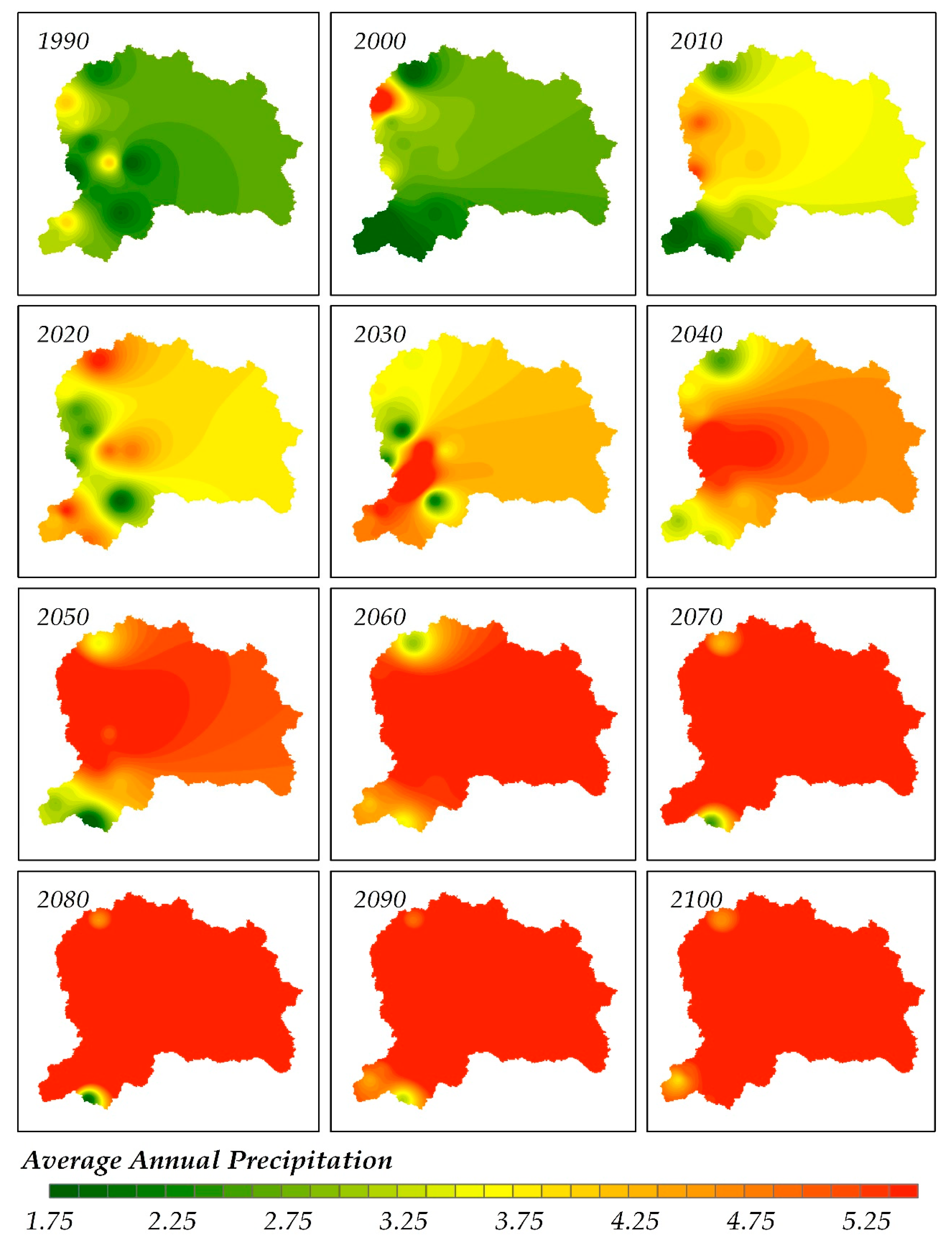
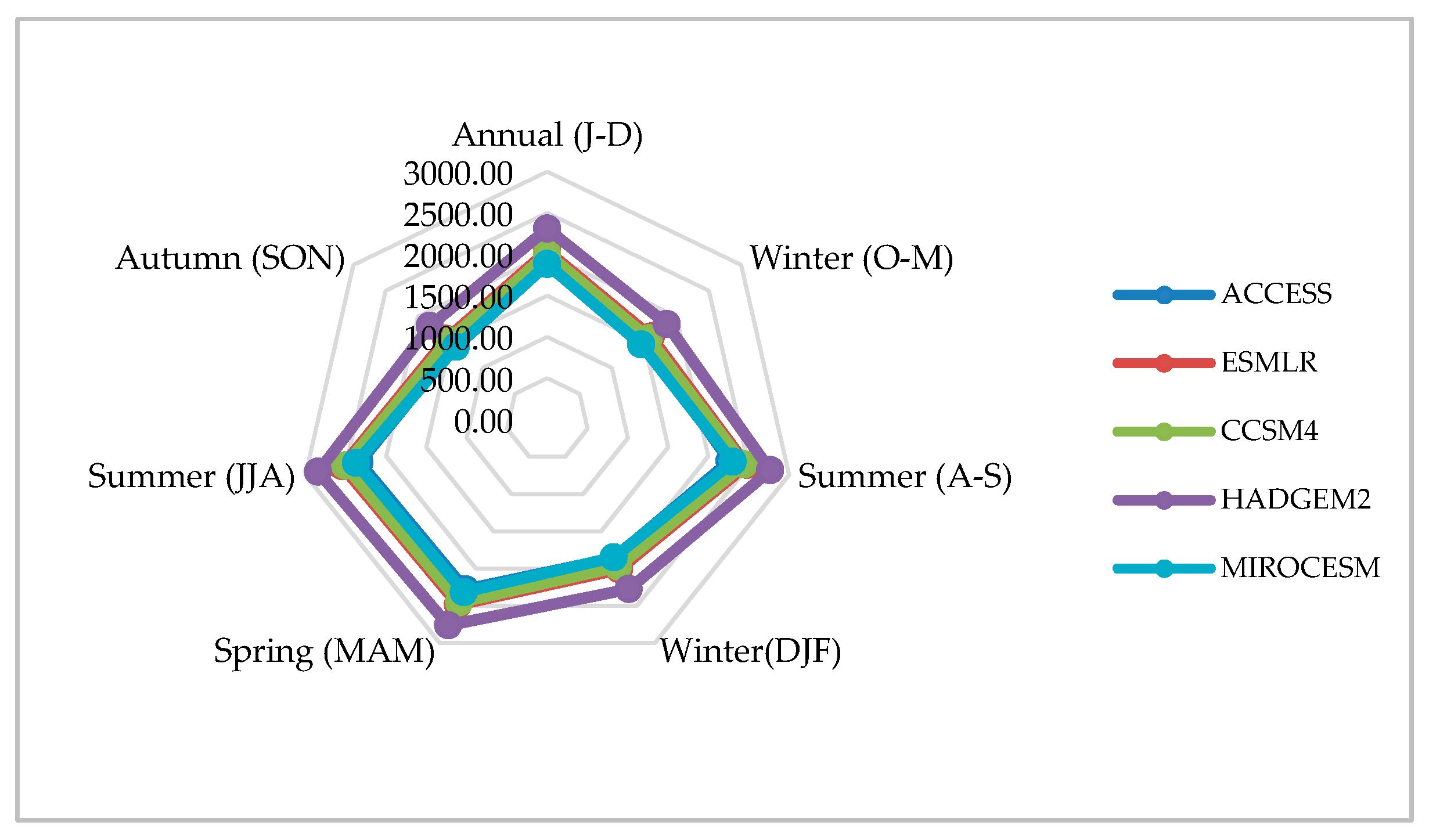
3.3. Seasonal Change in Temperature and Precipitation

The variation in mean seasonal rainfall is limited in spring and winter while shifting in rainfall is more during autumn and summer seasons for five GCMs. The rainfall during the moon-soon season is predicted to be more intense, while there will be a large increase in temperature; up to 8.4 °C. From Figure 7, it is concluded that in the 20th century the temperature is relatively less than in the 21st century; meanwhile, the temperature is increasing at a relatively steeper rate as compared with the previous period. In the year 1990, the average temperature of the whole watershed was 24.5 °C, whereas the expected average annual temperature for the 2030 scenario is 26.2 °C. It can be observed that there is almost a 1.7 °C increase in temperature in four decades. However, it can also be observed that in 2070, the average temperature will reach 29.54 °C, as there will be a rise of almost 3.34 °C in the next four decades. For 2100, the temperature will touch 32.08 °C, from which it can be observed that the temperature will rise to 2.54 °C during the period from 2070 to 2100. Considering RCP (4.5), it can be observed that temperature will tend to rise at a higher rate during the middle of the century, as compared to the end of the century.
Figure 7 revealed the average temperature from 1990 to 2100 within the transboundary Mangla Watershed. The best adopted downscaling technique for the watershed, i.e., distribution mapping downscaling, was used to predict these results. Figure 7 represents that the maximum rise in temperature till 2100 will be 8.9 °C. It is a large increase in temperature which will definitely increase evapotranspiration and also cause glaciers to melt and will severely affect freshwater resources in the future.
Figure 8 shows the projected change in precipitation (mm) over the Mangla watershed from the year 1990 to 2100. In 1990, there was less precipitation in most of the watershed, and it increases continuously in the future from 2021 to 2100. The northern part of the Mangla Watershed located at a higher altitude registered more rainfall as compared to the southern part of the watershed. In the late century, there will be more precipitation due to an increase in temperature. The increase in temperature ultimately causes evapotranspiration and precipitation to surge.
Figure 9a shows the average annual precipitation of ensembled GCM models [71] from 1981 to 2010 under three downscaling techniques for the RCP 4.5 radiative forcing emission scenario. The average annual precipitation under change factor downscaling ranges from 3.2 mm to 5.5 mm. The average annual precipitation from ensembled model output ranges from 2.78 mm to 4.89 mm under distribution mapping downscaling, and 2.54 mm to 9.4 mm under linear scaling. Figure 9b shows the GCMs ensembled average annual precipitation under RCP 8.5. The change factor downscaling ranges between 3.14 mm and 5.47 mm, distribution mapping ranges from 2.44 mm to 4.65 mm, and linear scaling ranges between 2.87 mm and 9.33 mm.
Figure 10 shows the GCMs ensembled average temperature trends from 1981 to 2100. The temperature under both RCPs showed an increasing trend. Figure 10a shows the change in Tmax and Tmin from 1981 to 2100 under the RCP 4.5 scenario. The increase in Tmax under change factor (CF) downscaling is 6.32 °C and an increase in Tmin is 5.45 °C. There is a 5.36 °C rise in Tmax and 4.34 °C in Tmin under the distribution mapping downscaling technique. In linear scaling, there is a 3.92 °C increase in Tmax and 2.78 °C in Tmin. Figure 10b shows the change in Tmax and Tmin under the RCP 8.5 scenario. The Tmax and Tmin were increased by 7.89 °C and 6.85 °C respectively under change factor downscaling and RCP 8.5. In distribution mapping, the Tmax was increased by 7.79 °C, whereas the Tmin was increased by 7.74 °C under RCP 8.5. The linear scaling downscaling has an increase of Tmax of 5.99 °C and a Tmin of 5.37 °C.

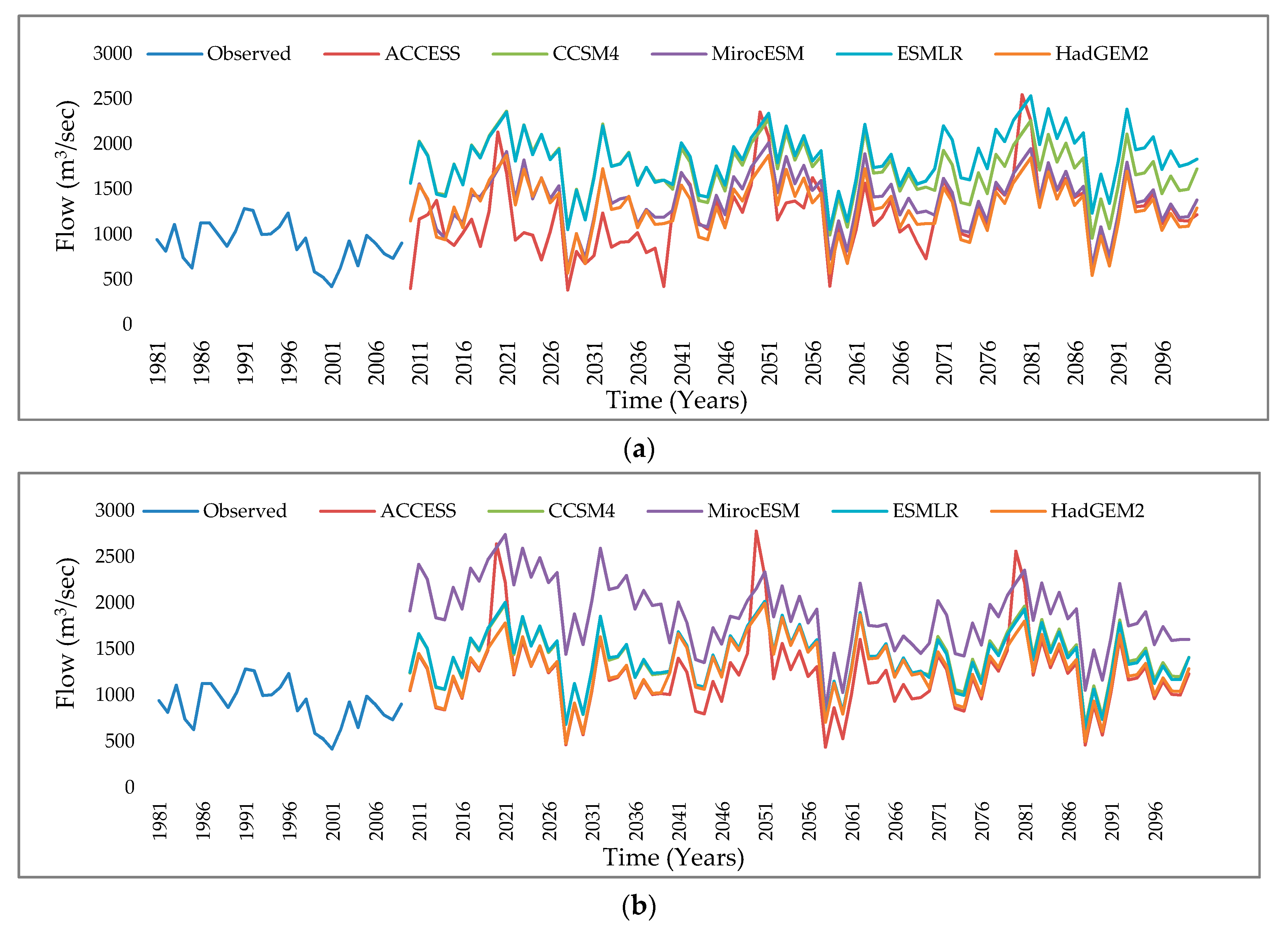
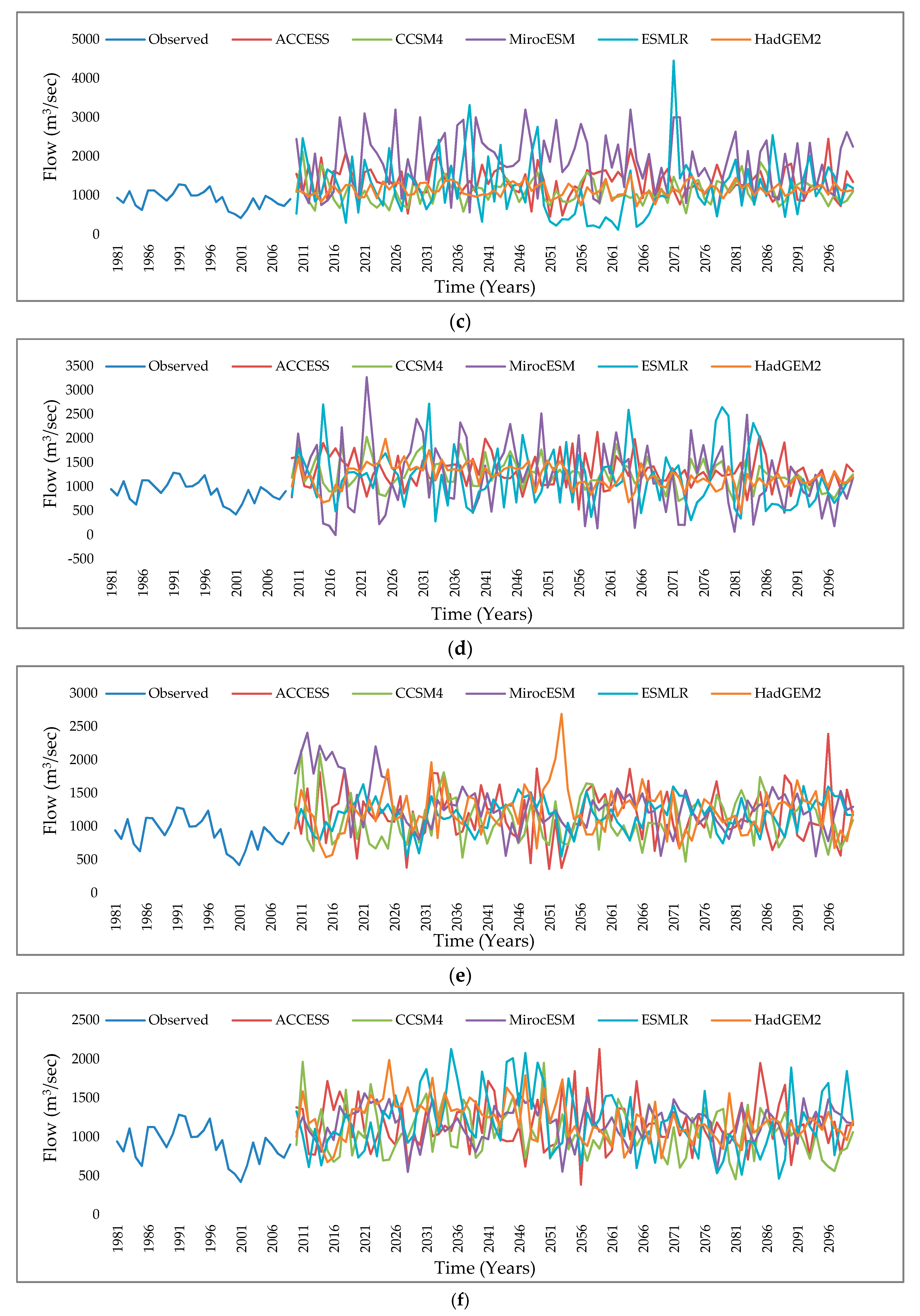
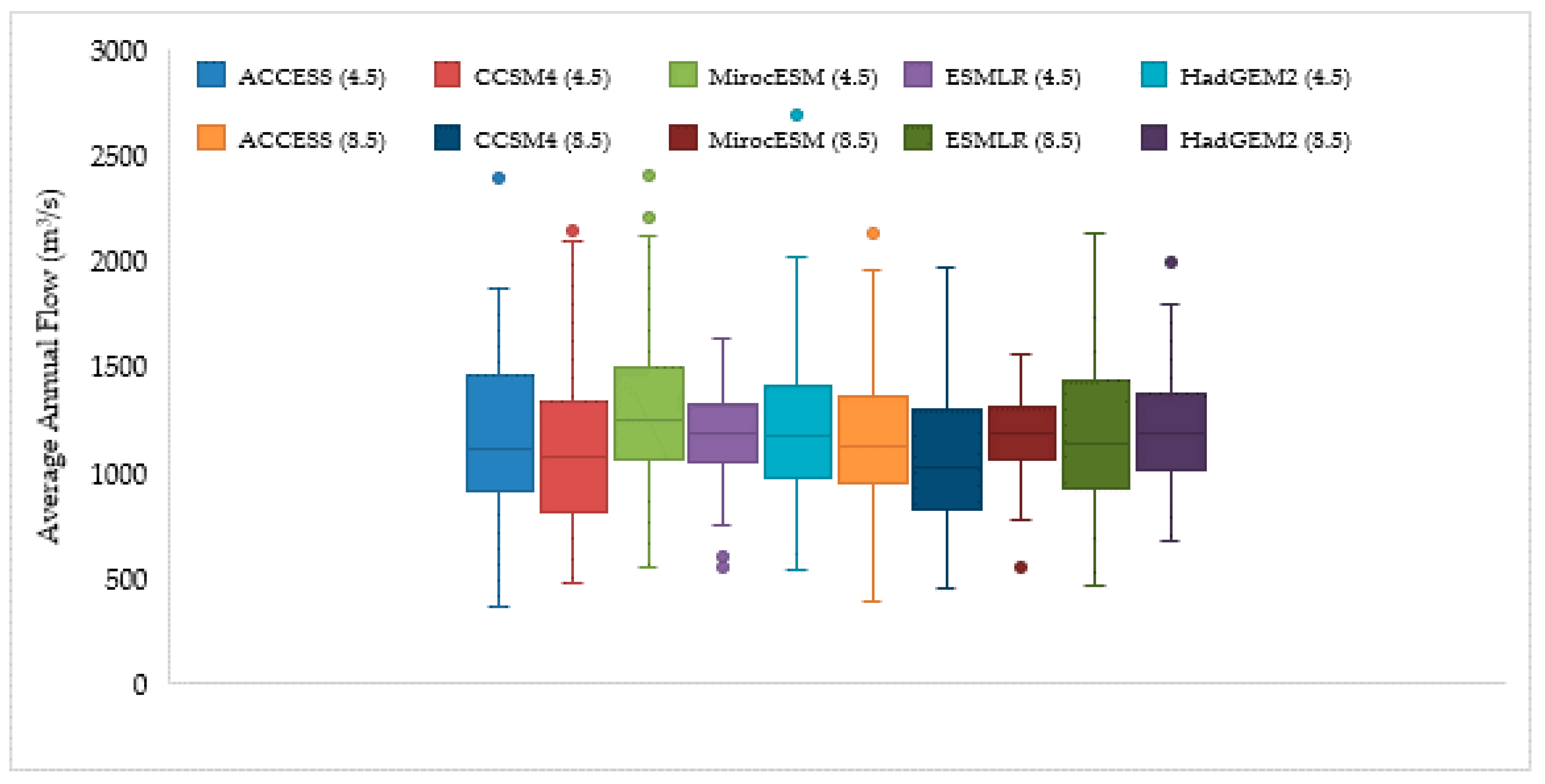
3.4. Future Flow Projection

The streamflow generation by applying CMIP5 GCMs data in SWAT is quite uncertain. The increase in streamflow on a larger scale has been observed in all five GCMs. The percentage increase in flow following RCP 4.5 can be observed in Table 7. In the summer season, the flow will tend to decrease, while in winter, it tends to rise. Both flood and drought scenarios can be observed in the prospect in the watershed. Using the global climatic model, ACCESS, from 2021 to 2039, the annual flow will tend to rise by 60.19%. The stream flows are predicted to rise by 87.62% during the years 2040–2069 and 97.17% from 2070–2099. During the summer season (June, July, and August), these flows tend to decrease considerably for 2021–2039 scenarios, as the flows will be 121.74% more than base period flows, whereas, from 2040–2069, scenarios showed a 62.35% decrease in streamflow as compared with the base period. In the last decade, the flows in summer will reach to 52.02%. Winter season (including December, January, and February) showed a remarkable increase in streamflow, 35.57% in 2021–2030, 154.25% in the mid-century, and 200.05% in the late century. The annual and seasonal flow exceedance percentage was described in Table 7, regarding five GCMs under RCP 4.5 during three periods; 2021 to 2039, 2040 to 2069, and 2070 to 2099. The annual flow will tend to increase up to 155.2%; the flow during winter will increase up to 186.29%. In summer, it will increase up to 121% and in autumn it will increase up to 175.97%. There is a maximum increase during the spring season which may lead to floods, and during the winter season, the streamflow tends to shrink, which may cause droughts. Flows will upsurge at an abrupt rate in the prospect. For instance, it is revealed that, through the year 2021 to 2040, because of ACCESS, the annual average flows will rise to 86.36%, while for the year 2030–2070, it will rise at a higher grade of 88.52%. The flow will upsurge by 110.55% in the course of the year 2070 to 2100. In the summer season, a decrease was observed, whereas, in spring and winter, flows are showing a remarkable increase. By studying the results of MIROCESM, it can be observed that, on an annual basis, streamflow will increase by 121.56% from 2021–2039, as compared with the base period 1981 to 2010. In the year 2040–2070, the streamflow will increase more and reach the peak value of 137.31%, and at the end of the century, it will touch 142.87%. In the summer season, stream flows are showing a decline, as in the first 30 years, the average streamflow is projected to be 107% more than the base streamflow; in the next period, it will decline to 99.13%, and in the year 2070–2099, it will decline by more than 97.95%.
Figure 11a shows the percentage increase in stream flows as compared with the base flow for the RCP 4.5 scenario by downscaling using the change factor technique. The streamflow under ACCESS increment ranges from −67.9% to 112.2%, ESMLR ranges from −12.2% to 111.3%, and CCSM4 ranges from −20.9% to 96.3%; HadGEM2 ranges from −54.6% to 56.1% and MirocESM ranges from −49.6% to 67.5%. In Figure 11b, an annual percentage increase in stream flows, as compared with the base flow by using the change factor downscaling technique under RCP 8.5, is presented. The extreme values for streamflow increase under ACCESS ranges from 9.03% to 243.2%, ESMLR arrays from 28.09% to 165.33%, CCSM4 ranges from 31.3% to 165.3%, HadGEM2 ranges from 28.09% to 166.8% and MirocESM series from 48.7% to 239.26%. Figure 11c shows an annual percentage increase in stream flows as compared with baseflow under the linear scaling downscaling technique for RCP 4.5. The extreme values for streamflow under ACCESS increment ranges from −54.3% to 145.3%, ESMLR ranges from −87.9% to 345.3%, CCSM4 ranges from −45.5% to 112.7%, HADGEM2 ranges from −27.9% to 53.9%, and MirocESM ranges from −51.7% to 220.3%. Figure 11d shows an annual percentage increase in stream flows as compared with the base flow by using linear scaling downscaling under RCP 8.5. The extreme values for streamflow under ACCESS increment range from −47.6% to 113.2%, ESMLR ranges from −72.0% to 172.3%, CCSM4 ranges from −33.5% to 103.3%, and HadGEM2 ranges from −54.2% to 99.4%. Figure 11e shows an annual percentage increase in stream flows as compared with the base flow by using distribution mapping downscaling under RCP 4.5. The extreme values for streamflow under ACCESS increment range from −63.7% to 139.2%, ESMLR ranges from 44.8% to 140.73%, CCSM4 ranges from −52.7% to 114.3%, HadGEM2 ranges from −46.3% to 168.9% and MirocESM ranges from −44.8% to 140.7%. Figure 11f shows an annual percentage increase in stream flows as compared with the base flow, by using distribution mapping downscaling under RCP 8.5. The extreme values for streamflow under ACCESS increment ranges from −61.5% to 112.7%, ESMLR ranges from −53.6% to 112.7%, and CCSM4 ranges from −54.3% to 96.6%, HadGEM2 ranges from 32.49% to 164.425% and MirocESM ranges from −45.7% to 56.9%. It is observed that the possibility of the appearance of low and high flow could be more leading in the prospect within the Mangla watershed following both RCP scenarios. However, average flows during the summer season were predicted to decrease by all five GCMs. This reduction in summer outflow is usually possible due to the reduction in average yearly precipitation. The difference in high outflow and outflow duration trajectories explains that the repetition of water abundance will further increase their quantities into the prospect that will generate plenty of administration obstacles in the watershed. Not only economic losses but also losses of life will be caused by flooding in the future.
Figure 12a shows average annual stream flows compared with the base flow for change factor downscaling and RCP 4.5 emission scenarios. The extreme values for streamflow under ACCESS ranges from 380 m3/s to 2547 m3/s, CCSM4 ranges from 958 m3/s to 2363 m3/s, MirocESM ranges from 604 m3/s to 2013 m3/s, ESMLR ranges from 1052 m3/s to 2533 m3/s, and HadGEM2 ranges from 544 m3/s to 1874 m3/s. Figure 12b future flow projection compared with the observed flow by using the change factor downscaling under the RCP (8.5) emission scenario. The extreme values for streamflow under ACCESS ranges from 440 m3/s to 2782 m3/s, CCSM4 ranges from 663 m3/s to 2003 m3/s, MirocESM ranges from 838 m3/s to 2743 m3/s, ESMLR ranges from 631 m3/s to 2019 m3/s, HADGEM2 ranges from 483 m3/s to 1994 m3/s. Figure 12c depicts the future flow projection compared with the observed flow by using linear scaling downscaling under RCP (4.5) emission scenario. The extreme values for streamflow under ACCESS range from 456 m3/s to 2453 m3/s, CCSM4 ranges from 545 m3/s to 2127 m3/s, MirocESM ranges from 483 m3/s to 3200 m3/s, ESMLR ranges from 121 m3/s to 4454 m3/s, and HadGEM2 ranges from 720 m3/s to 1539 m3/s. ESMLR predicts very high flows in the year 2071 during the summer season. Figure 12d shows the future flow projection compared with the observed flow by using the linear scaling downscaling under RCP (8.5) emission scenario. The extreme values for streamflow under ACCESS range from 524 m3/s to 2132 m3/s, CCSM4 ranges from 668 m3/s to 2031 m3/s, MirocESM ranges from 136 m3/s to 3271 m3/s, ESMLR ranges from 276 m3/s to 2721 m3/s, and HadGEM2 ranges from 460 m3/s to 1990 m3/s. Figure 12e shows future flow projection compared with the observed flow, by using distribution mapping downscaling under the RCP (4.5) emission scenario. The extreme values for streamflow under ACCESS ranges from 363 m3/s to 2392 m3/s, CCSM4 ranges from 473 m3/s to 2142 m3/s, MirocESM ranges from 553 m3/s to 2408 m3/s, ESMLR ranges from 545 m3/s to 1634 m3/s, and HADGEM2 ranges from 537 m3/s to 2689 m3/s. Figure 12f shows the future flow projection compared with the observed flow, by using the distribution mapping downscaling of global climate models under the RCP (8.5) emission scenario. The extreme values for streamflow under ACCESS ranges from 385 m3/s to 2127 m3/s, CCSM4 ranges from 456 m3/s to 1966 m3/s, MirocESM ranges from 550 m3/s to 1562 m3/s, ESMLR ranges from 464 m3/s to 2127 m3/s, and HADGEM2 ranges from 675 m3/s to 1990 m3/s.
The multi-model ensemble means (EM) method was used to ensemble the five GCMs time series data under three types of downscaling techniques and two different emission scenarios. Figure 13 revealed that in EM, under change factor downscaling, GCMs are projecting high flows, ranges between 735 m3/s to 2169 m3/s under RCP 4.5 and 662 m3/s to 2149 m3/s under the RCP 8.5 scenario. In linear scaling downscaling, the streamflow ranges between 776 m3/s and 2246 m3/s under the RCP 4.5 scenario, whereas it is from 787 m3/s to 1789 m3/s under the RCP 8.5 scenario. The distribution mapping downscaling ranges between 828 m3/s to 1591 under RCP 4.5 and 831 m3/s to 1516 m3/s under the RCP 8.5 scenario. The observed flow ranges between 420 m3/s and 1285 m3/s.
Figure 14 shows the average annual flow (January to December); winter (October to March), Summer (August to September); Winter (December, January, and February); Spring (March, April, and May); Summer (June, July, and August) and Autumn (September, October, and November) during the year 2021 to 2100. Figure 14 revealed that there will be more streamflow during the summer season, whereas there will be very little streamflow during the autumn season. The streamflow during the summer season is relatively more due to the melting of glaciers but as we proceed to the next period 2040–2069 the streamflow during the summer season show a remarkable declining trend. A large volume of water in streams is observed in the spring season and it will tend to rise in the future. By considering distribution mapping, the average annual flows are 1887 m3/s flows during the autumn season, 1435 m3/s in the summer season 2263 m3/s, and in the spring season, stream flows will be 2280 m3/s. There are a few uncertainties in the generated flows because the climatic data of temperature and precipitation from several GCMs vary due to their different resolutions. All of the five GCM are predicting huge stream flows during the spring season, while there will be very little streamflow during the autumn season.
The box-plot represents the value of Q0 as lower extreme, Q25% as lower quartile, Q50% as median, Q75% as upper quartile, and Q100% as the upper extreme of average annual flows. Figure 15 shows that the lower and upper extremes of ESMLR under RCP-4.5 are 464 (m3/s) and 2127 respectively, having a median flow of 1136 (m3/s). Similarly, the lower and upper extremes of MirocESM 770 (m3/s) and 1562 (m3/s) respectively, and median flow of 1188 (m3/s). HadGEM2 with one upper outlier point has a lower extreme, 675 (m3/s), and an upper extreme, 1793 (m3/s); the median flows of ACCESS, CCSM4, MirocESM, ESMLR, HadGEM2 are 1126 (m3/s), 1024 (m3/s), 1188 (m3/s), 1136 (m3/s) and 1191 (m3/s), respectively. Under the RCP-8.5 scenario, Figure 15 also depicts that the lower extreme for ACCESS is 363 (m3/s) and the upper extreme is 1870, whereas (m3/s). GCMs ESMLR has a minimum range of 746 (m3/s) to 1633 (m3/s) and two outlier points. The upper extreme of MirocESM is 2119 (m3/s) and the lower extreme is 552 (m3/s). The median streamflow values of ACCESS, CCSM4, MirocESM, ESMLR and HadGEM2 are 1112 (m3/s), 1077 (m3/s), 1247 (m3/s), 1181 (m3/s), and 1175 (m3/s) respectively.
Table A1 represents the peak, mean, and low streamflow from the year 2021 to 2100 under the RCP-4.5 emission scenario. The peak flows occur commonly in the summer season (during June, July, and August) due to the melting of snow from the northern part of the watershed, and low flows usually occur during the winter season due to less snow melting. HadGEM2 depicts the maximum value of 8520 m3/s for peak flows from 2051–2060 under RCP 4.5 among all GCMs, followed by ACCESS with a value of 8342 m3/s from 2091–2100. The maximum value of median flows has been found during the 2021–2030 decade for MirocESM with a value of 1182 m3/s followed by 2031–2040 decade for the same GCM, and ACCESS indicates the minimum value of 714.4 m3/s from 2091–2100 under RCP 4.5. Furthermore, the minimum and maximum values of low flows can be found for HadGEM2 from 2031–2040 and 2061–2070, respectively, among all the five GCMs.
Table A2 represents the peak, mean, and low streamflow from the year 2021 to 2100 under RCP-8.5 for five GCMs. Under RCP-8.5, the peak flow of GCM varies from 2406 (HadGEM2 2071–2080) to 8890 m3/s (ESMLR from 2061–2070), median flow varies from 525.9 (ESMLR from 2081–2090) to 1202 m3/s (HadGEM2 from 2041–2050) and the low flow varies from 15.11 (ESMLR from 2031–2040) to 241.9 m3/s (MirocESM from 2091–2100) for all GCMs based on the decadal data. If we talk about these GCMs at the individual level, the peak flows vary between a range of 4004–735, 3472 to 6981, 2406–6930, 4003–8890 and 3613–7395 m3/s for ACCESS, CCSM4, HadGEM2, ESMLR, and MirocESM, respectively, median flows vary between 741–920, 641–909, 851–1202, 525–961 and 817–1130 m3/s s for ACCESS, CCSM4, HadGEM2, ESMLR, and MirocESM, respectively, and low flows vary between 81.86–222.6, 39.97–225.9, 51.66–333, 15.11–93.97 and 91.36–241.9 m3/s, for ACCESS, CCSM4, HadGEM2, ESMLR, and MirocESM, respectively.

4. Discussion

In this study, future climate change was assessed under RCP (8.5) and RCP (4.5) emission scenarios. Change of temperature and precipitation and their probable effects on water resources at Mangla Watershed was studied on a broad spectrum. Five GCMs, along with their ensembles, were selected, and three types of downscaling techniques were compared to estimate the change in precipitation and temperature. After a comparison of these downscaling techniques with base data, it was concluded that the distribution mapping is the best downscaling technique to study climatic parameters within the watershed, however, linear scaling downscaling was found to be a less effective downscaling technique, as the results are in close agreement with previous studies [51]. Downscaled data were used to generate stream flows using a semi-distributed hydrological model SWAT. In this research, evapotranspiration was neglected due to data scarcity and unreliability. Observed data were gathered from seventeen metrological stations, five of them in the Indian region. The scarcity of metrological stations within Mangla Watershed can cause the low performance of the calibration. The land use classification and soil type were kept constant throughout the simulations. This type of assumption can affect the prediction of streamflow. Uncertainty exists as a well-known problem toward most of the hydrological modeling considerations, particularly on large scales. The bulk part of these uncertainties appears in the forecasted precipitation and temperature datasets, due to the distinctive resolutions of several GCMs. The streamflow generated by using these datasets also shows uncertainties. In the prospect, as interpreted by [31], the projection of climatic parameters using CMIP5 GCM is considerably uncertain. In the present research, five GCMs of distinct variation in resolutions are used to predict future climatic scenarios. Many uncertainties were found in the maximum and minimum temperature, as well as in rainfall after using three downscaling techniques applied on CMIP5 GCMs. The uncertainties occurred in maximum temperature using the RCP 4.5 scenario ranges between 2.58 °C and 5.30 °C, while in minimum temperature, it ranges between 0.8°C and 2.0°C. These uncertainties under the RCP 8.5 scenario are even more probable. The maximum temperature under the RCP 8.5 scenario ranges between 4.33 °C and 8.90 °C, whereas the minimum temperature ranges between 3.10 °C to 8.60 °C [21]. These temperature variations ultimately affect the amount of precipitation. The percentage increase in precipitation compared to the baseline period ranges between 45 to 128.4% under the RCP 4.5 scenarios and 92 to 180.3% in the RCP 8.5 scenario. As predicted by [72], it is hard to exactly predict the climatic variables, particularly rainfall, and consequently, uncertainties in predicted temperature and rainfall will lead to uncertainties in streamflow [31]. The results of five GCMs under both RCPs 4.5 and RCP 8.5 scenarios, illustrates that the change in temperature and precipitation frequencies will affect the water resources and streamflow within the transboundary, directly or indirectly. Besides climate change, other anthropogenic changes can also have a significant impact on streamflow, such as future management practices and land-use change significantly influencing water availability [61,73].
The projected GCMs show an increase in the precipitation amount in the study area compared to base years and are in close agreement with previous studies [21,24,74]. The rainfall is greatly affected by various transmission systems, such as monsoons [75]. The moisture transportation, inter-annual, and inter-decadal change of the monsoon are the principal agents that can induce an accession in the rainfall frequencies in the Indus basin region [45]. An increase in precipitation amount is also vulnerable to temperature change at a different inter-annual and inter-decadal time [29]. These factors are performing a major role in the increase of precipitation; further investigations by performing different climatic modeling techniques ought to be carried in the prospect to study these aspects in more detail. The projected increase in precipitation and temperature tends to influence the streamflow within the transboundary Mangla dam watershed and is in close agreement with the previous work carried out in the study area [21,24,45]. This increase in streamflow in the rivers will tend to cause floods [76], so several preventions, such as the construction of new dams, are strongly recommended. The results of this study are consistent with the results of precipitation and temperature in the past [45]. These projected climatic variables and stream flows could be valuable for policymakers and water resource administrators for the proper administration of water reserves. Some of the predicted streamflows showed a large increase that may cause floods in the prospect, to avoid these floods this study can be valuable for water resource planners for the management of water resources construction of new water storage structures, and modernizing the designs and storage capabilities of existing dams.

5. Conclusions

Pakistan stands among one of the countries with significant and more prominent water stress, and its existing water resources are extremely vulnerable to climate change. In this investigation, the possible consequences of climate change on water reserves in the Mangla Watershed have been evaluated under RCP 4.5 and RCP 8.5 scenarios using the outputs of five GCMs. The forecasts for climatic variables and their probable influences on water resources within the boundary of Mangla Watershed were examined up to the year 2099. Under CMIP5, five GCMs and their ensembles were used, considering RCP 4.5 and RCP 8.5 emission scenarios to forecast temperature, precipitation, and streamflow within the watershed, to attain substantial precipitation, maximum and minimum temperature data series following various climate change situations. Change factor, linear scaling, and distribution mapping downscaling techniques were exercised to downscale the future projections of climatic parameters. Furthermore, the mentioned three downscaling techniques were inter-compared and decided the best downscaling technique for the watershed. The hydrological model SWAT, after calibration, was applied to produce streamflow based on the values of the climatic parameters that were downscaled by the specified downscaling techniques. Subsequently, the streamflow generated by using these downscaled data in SWAT was analyzed, comprehensively, for all five models and their ensembles. The several noticeable results extracted from this research were compiled as subsequently:
  • The results regarding calibration and validation criteria, i.e., NSE, PBIAS, and R2, are satisfactory within the monthly period by incorporating elevation bands. The calibrated hydrological model SWAT precisely re-generates streamflow within the Mangla Watershed.
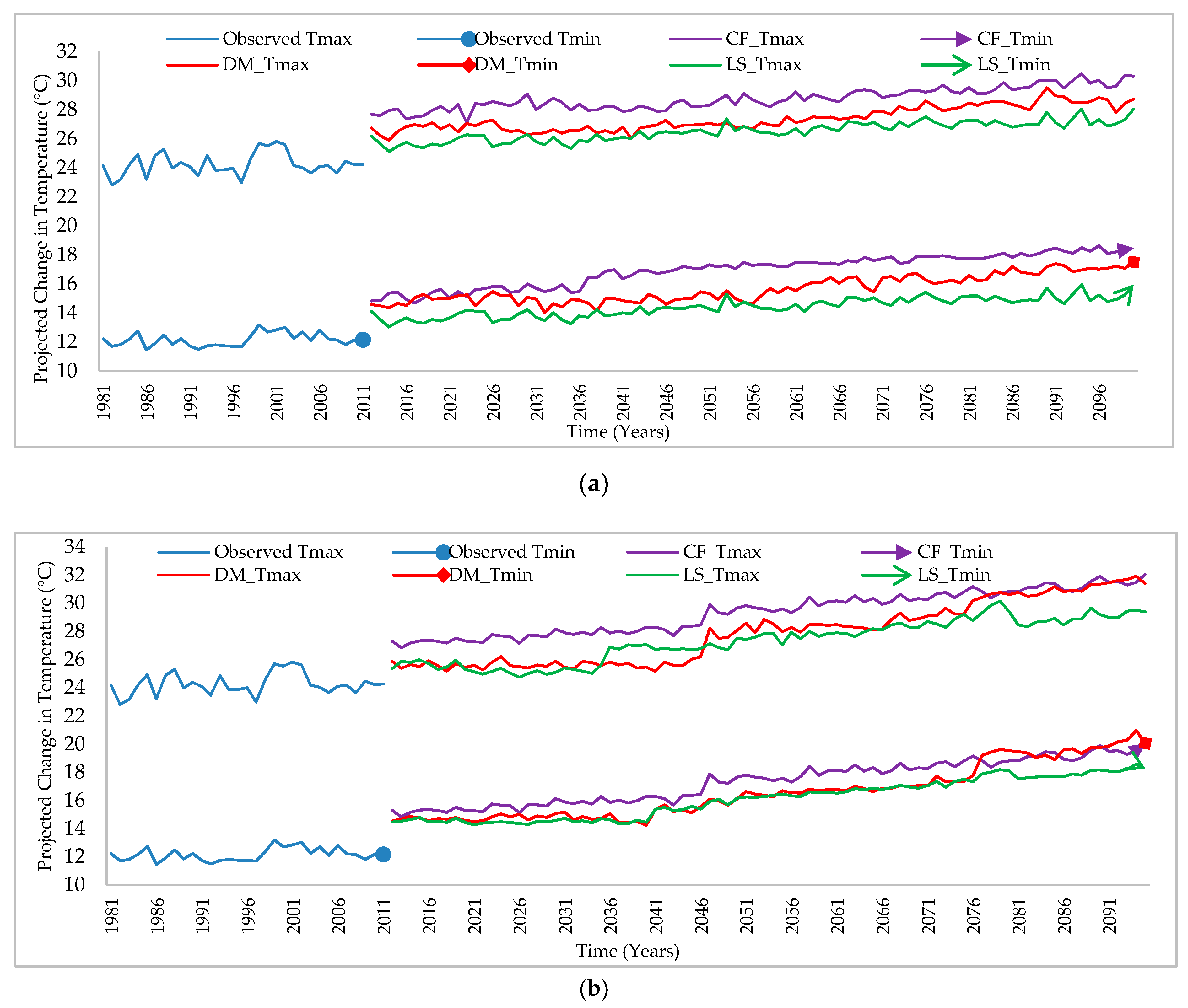
  • Maximum temperature and minimum temperature are projected to increase in the future from 2021 to 2099 for all five GCMs, under both RCP (4.5) and RCP (8.5) emission scenarios.
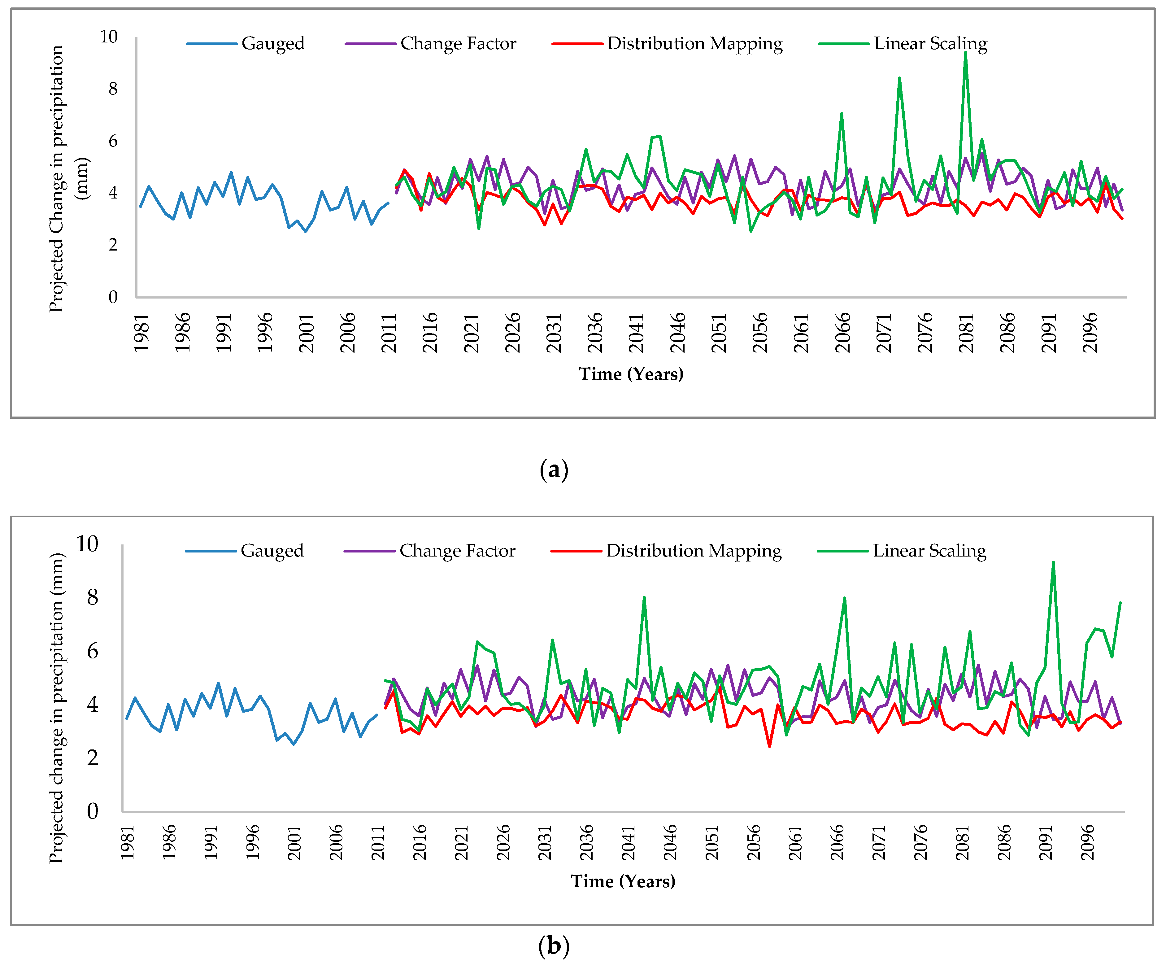
  • The projected precipitation is more uncertain and obscure. All five GCMs and their ensemble are predicting an increase in precipitation frequencies from June to September within the Mangla Watershed with a significant increase of (219%) in June.
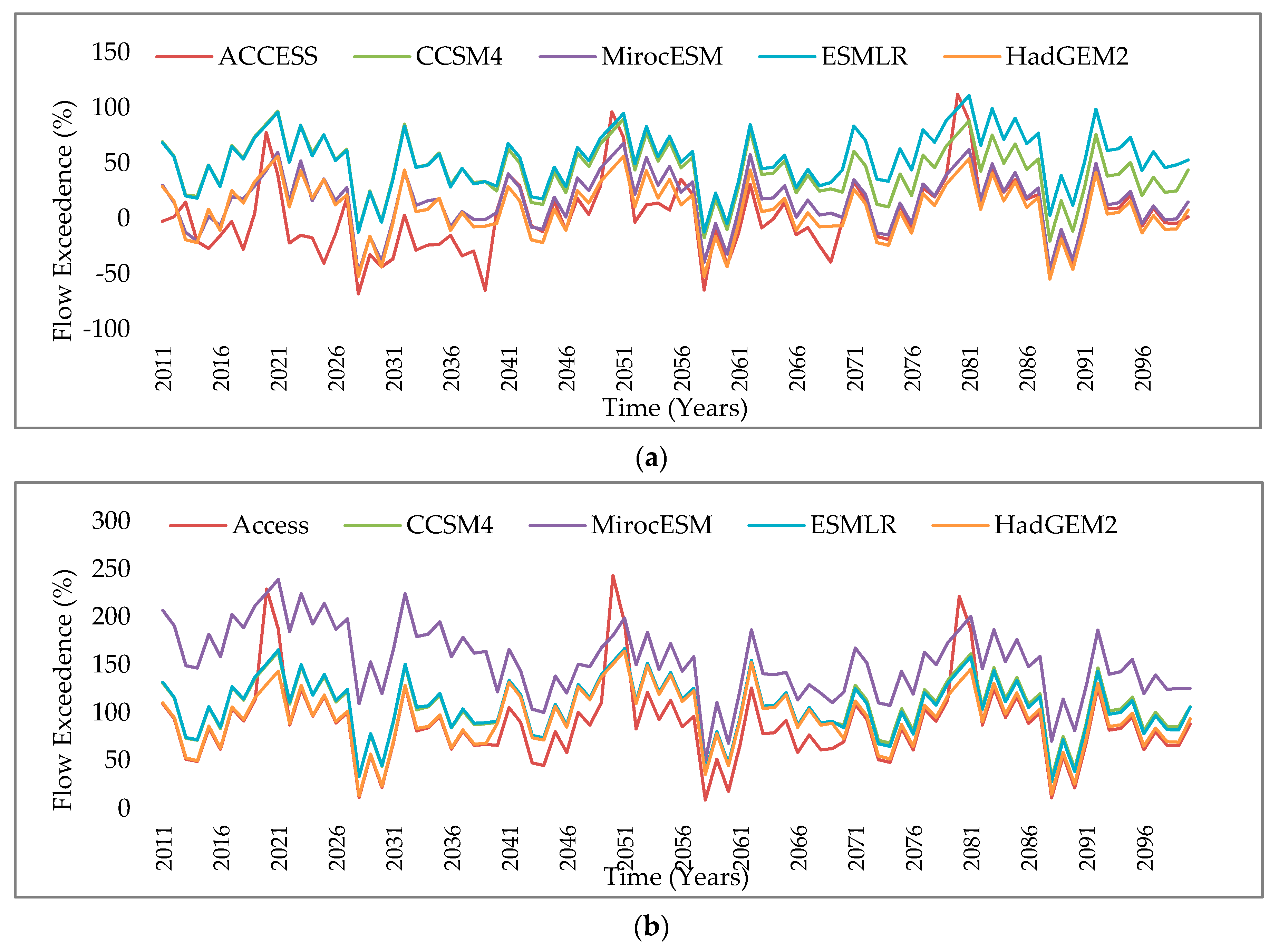
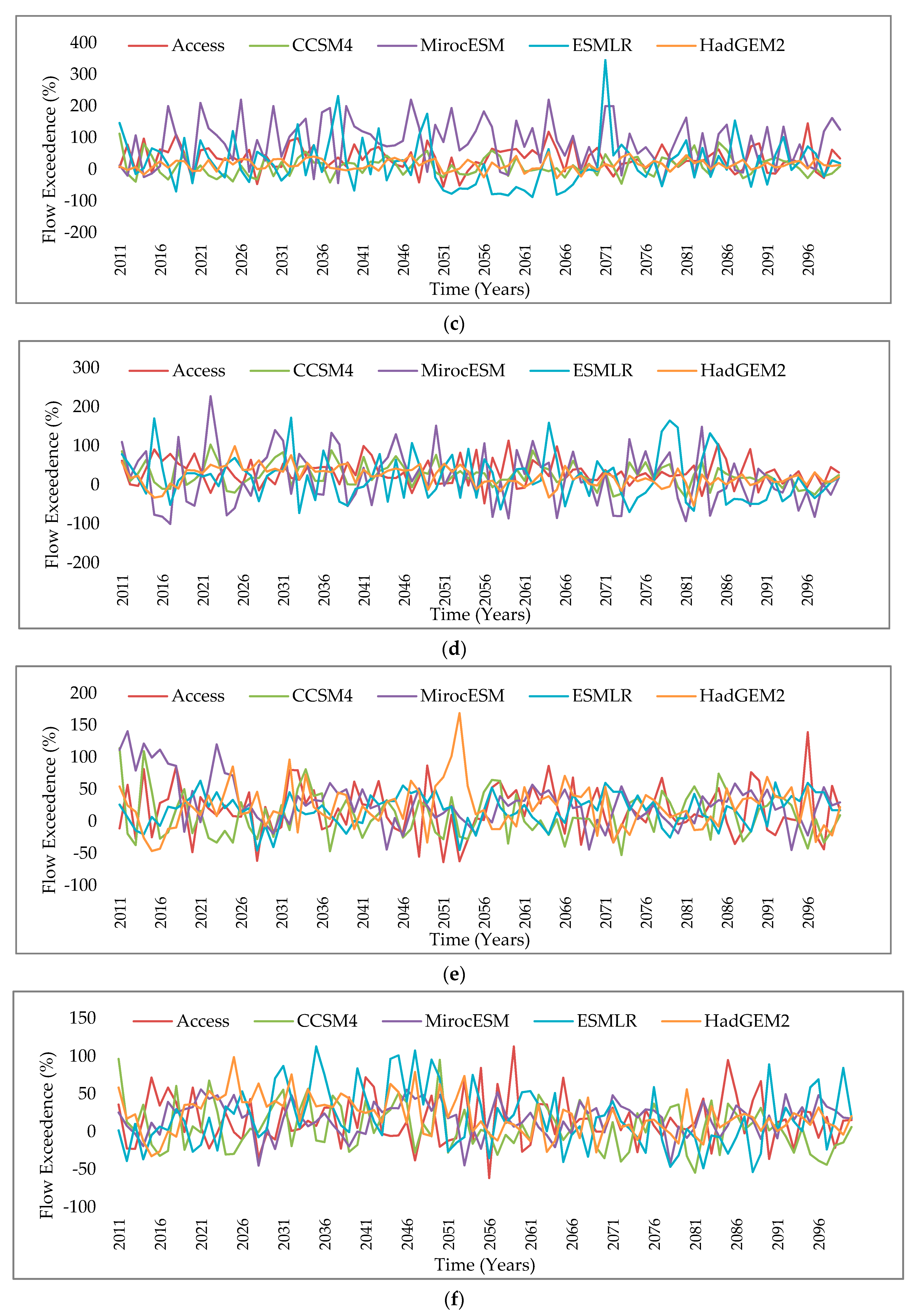
  • The projected average annual flow will increase constantly for all five GCMs and their ensemble, especially in the Spring season with a 193% increase, but there will be a decrease in the streamflow during the autumn season. Moreover, there will be an excess of high flows and low flow events for the projected flows.
Hence, based on these outcomes, to predict climatic parameters in the future, a more certain GCMs ensemble scenario could be used. An increase in flow will cause high flood risk in the watershed. By applying good management practices and by constructing dams and reservoirs, Pakistan may be able to generate more hydropower and also produce more food for its residents. The principal outcome of the research is that the Mangla watershed will be expected to face more flooding in the future, and average flows are supposed to decrease. The maximum temperature, minimum temperature, and precipitation peak will also tend to increase in the future. The outcomes of this research are helpful for climate change researchers, development planners, and policymakers toward designing and accomplishing suitable water administration systems to mitigate the influences of climate change.

Author Contributions

Conceptualization, H.H., M.Z., S.L.; Data curation, H.H., M.Z., and M.U.; Formal analysis, H.H., and M.Y.; Funding acquisition, S.L.; Investigation, H.H. and M.A.; Methodology, H.H., M.Z., M.N.A.; Project administration, H.H., M.Z., S.L., M.W., J.N.C.; Resources, M.Z., S.L., M.U., J.N.C., and M.S.; Software, M.Z., M.S., and M.W.; Supervision, M.Z., S.L., M.U., and J.N.C.; Validation, M.Z., M.U., and M.S.; Visualization, M.Z., M.U., and M.S.; Writing—original draft, H.H., AND M.Z.; Writing—review and editing., M.Z., M.N.A., and M.S. All authors have read and agreed to the published version of the manuscript.

Funding

This research was funded by joint Research project of National Natural Science Foundation of China and International Center for Integrated Mountain Development NSFC-ICIMOD (Grant No. 41761144075), China Postdoctoral Science Foundation (Grant No. 209071) and Yunnan University (YJRC3201702).

Acknowledgments

We are thankful to the Pakistan Meteorological Department (PMD) and Water and Power Development Authority (WAPDA) of Pakistan for providing the in situ data. Moreover, we are thankful to the open access department at the University of Rostock for their willingness to pay article processing charges.

Conflicts of Interest

The authors declare no conflict of interest.

Appendix A

Table A1. Peak, median and low flows (2021–2100) under RCP-4.5.
GCMsACCESSCCSM4HadGEM2ESMLRMirocESM
YearsPeak Flow
(m3/s)
Median Flow
(m3/s)
Low Flow
(m3/s)
Peak Flow
(m3/s)
Median Flow
(m3/s)
Low Flow
(m3/s)
Peak Flow
(m3/s)
Median Flow
(m3/s)
Low Flow
(m3/s)
Peak Flow
(m3/s)
Median Flow
(m3/s)
Low Flow
(m3/s)
Peak Flow
(m3/s)
Median Flow
(m3/s)
Low Flow
(m3/s)
2021–203036037637339617481606730812514316111910053901182141
2031–20403798956119465787881579576121422893811055441120302
2041–20505560875135504081413558858862656831134173526389795
2051–2060416373810772307881358520977564898910965577976156
2061–2070494799195606073114859951122372564899515752581057160
2071–2080596292012648738445733908766740821034171410589596
2081–2090758189514351269201065813101819336888767155231101315
2091–21008342714985675766142435710236573881097217523192894
Table A2. Peak, median and low flows (2021–2100) under RCP-8.5.
GCMsACCESSCCSM4HadGEM2ESMLRMirocESM
YearsPeak Flow
(m3/s)
Median Flow
(m3/s)
Low Flow
(m3/s)
Peak Flow
(m3/s)
Median Flow
(m3/s)
Low Flow
(m3/s)
Peak Flow
(m3/s)
Median Flow
(m3/s)
Low Flow
(m3/s)
Peak Flow
(m3/s)
Median Flow
(m3/s)
Low Flow
(m3/s)
Peak Flow
(m3/s)
Median Flow
(m3/s)
Low Flow
(m3/s)
2021–203040048371134870845406930110819344398958648931046101
2031–2040448786215256818861404732105352847371415361388397
2041–205049879202233775789138644112026682205771856681123173
2051–20607335884116698179817448119631058510712152489190697
2061–2070550591114334729092264648778688890767195639993161
2071–208046308151705367629111240610113336969647184994895120
2081–20905068917824476679176421689566400352634425881891
2091–2100621174112441856429333001050706651961947395943242

References

  1. Scott, D.; Hall, C.M.; Gössling, S. A review of the IPCC Fifth Assessment and implications for tourism sector climate resilience and decarbonization. J. Sustain. Tour. 2016, 24, 8–30. [Google Scholar] [CrossRef]
  2. Hussain Sargana, M.; Saud, M. Pakistan’s Internal Security Dynamics: Way Forward. J. Peace Dev. Commun. 2019, 3, 1–26. [Google Scholar] [CrossRef]
  3. Stocker, T.F.; Qin, D.; Plattner, G.K.; Tignor, M.M.B.; Allen, S.K.; Boschung, J.; Nauels, A.; Xia, Y.; Bex, V.; Midgley, P.M. Climate Change 2013 the Physical Science Basis: Working Group I Contribution to the Fifth Assessment Report of the Intergovernmental Panel on Climate Change; Cambridge University Press: Cambridge, UK, 2013. [Google Scholar]
  4. Bolch, T. Hydrology: Asian glaciers are a reliable water source. Nature 2017, 545, 161–162. [Google Scholar] [CrossRef] [Green Version]
  5. Lutz, A.F.; Immerzeel, W.W.; Shrestha, A.B.; Bierkens, M.F.P. Consistent increase in High Asia’s runoff due to increasing glacier melt and precipitation. Nat. Clim. Chang. 2014, 4, 587–592. [Google Scholar] [CrossRef] [Green Version]
  6. Deng, H.; Chen, Y.; Wang, H.; Zhang, S. Climate change with elevation and its potential impact on water resources in the Tianshan Mountains, Central Asia. Glob. Planet. Chang. 2015, 135, 28–37. [Google Scholar] [CrossRef]
  7. Taylor, K.E.; Stouffer, R.J.; Meehl, G.A. An overview of CMIP5 and the experiment design. Bull. Am. Meteorol. Soc. 2012, 93, 485–498. [Google Scholar] [CrossRef] [Green Version]
  8. Muerth, M.J.; Gauvin St-Denis, B.; Ricard, S.; Velázquez, J.A.; Schmid, J.; Minville, M.; Caya, D.; Chaumont, D.; Ludwig, R.; Turcotte, R. On the need for bias correction in regional climate scenarios to assess climate change impacts on river runoff. Hydrol. Earth Syst. Sci. 2013, 17, 1189–1204. [Google Scholar] [CrossRef] [Green Version]
  9. Teng, J.; Potter, N.J.; Chiew, F.H.S.; Zhang, L.; Wang, B.; Vaze, J.; Evans, J.P. How does bias correction of regional climate model precipitation affect modelled runoff? Hydrol. Earth Syst. Sci. 2015, 19, 711–728. [Google Scholar] [CrossRef] [Green Version]
  10. Christensen, J.H.; Boberg, F.; Christensen, O.B.; Lucas-Picher, P. On the need for bias correction of regional climate change projections of temperature and precipitation. Geophys. Res. Lett. 2008, 35. [Google Scholar] [CrossRef]
  11. Maurer, E.P.; Hidalgo, H.G. Utility of daily vs. monthly large-scale climate data: An intercomparison of two statistical downscaling methods. Hydrol. Earth Syst. Sci. 2008, 12, 551–563. [Google Scholar] [CrossRef] [Green Version]
  12. Mbaye, M.L.; Haensler, A.; Hagemann, S.; Gaye, A.T.; Moseley, C.; Afouda, A. Impact of statistical bias correction on the projected climate change signals of the regional climate model REMO over the Senegal River Basin. Int. J. Climatol. 2016, 36, 2035–2049. [Google Scholar] [CrossRef] [Green Version]
  13. Fowler, H.J.; Blenkinsop, S.; Tebaldi, C. Linking climate change modelling to impacts studies: Recent advances in downscaling techniques for hydrological modelling. Int. J. Climatol. 2007, 27, 1547–1578. [Google Scholar] [CrossRef]
  14. Di Luca, A.; de Elía, R.; Laprise, R. Potential for small scale added value of RCM’s downscaled climate change signal. Clim. Dyn. 2013, 40, 601–618. [Google Scholar] [CrossRef] [Green Version]
  15. Kotlarski, S.; Keuler, K.; Christensen, O.B.; Colette, A.; Déqué, M.; Gobiet, A.; Goergen, K.; Jacob, D.; Lüthi, D.; Van Meijgaard, E.; et al. Regional climate modeling on European scales: A joint standard evaluation of the EURO-CORDEX RCM ensemble. Geosci. Model Dev. 2014, 7, 1297–1333. [Google Scholar] [CrossRef] [Green Version]
  16. Gellens, D.; Roulin, E. Streamflow response of Belgian catchments to IPCC climate change scenarios. J. Hydrol. 1998, 210, 242–258. [Google Scholar] [CrossRef]
  17. Chen, J.; Brissette, F.P.; Chaumont, D.; Braun, M. Performance and uncertainty evaluation of empirical downscaling methods in quantifying the climate change impacts on hydrology over two North American river basins. J. Hydrol. 2013, 479, 200–214. [Google Scholar] [CrossRef]
  18. Pervez, M.S.; Henebry, G.M. Assessing the impacts of climate and land use and land cover change on the freshwater availability in the Brahmaputra River basin. J. Hydrol. Reg. Stud. 2015, 3, 285–311. [Google Scholar] [CrossRef] [Green Version]
  19. Zhang, Y.; You, Q.; Chen, C.; Ge, J. Impacts of climate change on streamflows under RCP scenarios: A case study in Xin River Basin, China. Atmos. Res. 2016, 178–179, 521–534. [Google Scholar] [CrossRef]
  20. Wilby, R.L.; Dawson, C.W.; Barrow, E.M. SDSM - A decision support tool for the assessment of regional climate change impacts. Environ. Model. Softw. 2002, 17, 145–157. [Google Scholar] [CrossRef]
  21. Mahmood, R.; Babel, M.S. Evaluation of SDSM developed by annual and monthly sub-models for downscaling temperature and precipitation in the Jhelum basin, Pakistan and India. Theor. Appl. Climatol. 2013, 113, 27–44. [Google Scholar] [CrossRef]
  22. Maraun, D.; Wetterhall, F.; Ireson, A.M.; Chandler, R.E.; Kendon, E.J.; Widmann, M.; Brienen, S.; Rust, H.W.; Sauter, T.; Themel, M.; et al. Precipitation downscaling under climate change: Recent developments to bridge the gap between dynamical models and the end user. Rev. Geophys. 2010, 48, 32–41. [Google Scholar] [CrossRef]
  23. Sachindra, D.A.; Perera, B.J.C. Statistical downscaling of general circulation model outputs to precipitation accounting for non-stationarities in predictor-predictand relationships. PLoS ONE 2016, 11, 67–78. [Google Scholar] [CrossRef] [PubMed]
  24. Garee, K.; Chen, X.; Bao, A.; Wang, Y.; Meng, F. Hydrological modeling of the upper indus basin: A case study from a high-altitude glacierized catchment Hunza. Water 2017, 9, 17. [Google Scholar] [CrossRef]
  25. Tahir, A.A.; Adamowski, J.F.; Chevallier, P.; Haq, A.U.; Terzago, S. Comparative assessment of spatiotemporal snow cover changes and hydrological behavior of the Gilgit, Astore and Hunza River basins (Hindukush–Karakoram–Himalaya region, Pakistan). Meteorol. Atmos. Phys. 2016, 128, 793–811. [Google Scholar] [CrossRef]
  26. Ul Hasson, S.; Böhner, J.; Lucarini, V. Prevailing climatic trends and runoff response from Hindukush-Karakoram-Himalaya, upper Indus Basin. Earth Syst. Dyn. 2017, 8, 337–355. [Google Scholar] [CrossRef] [Green Version]
  27. DR, A.; HJ, F. Erratum to: Using meteorological data to forecast seasonal runoff on the River Jhelum, Pakistan. J. Hydrol. 2009, 364, 200–229. [Google Scholar] [CrossRef]
  28. Amin, A.; Nasim, W.; Mubeen, M.; Sarwar, S.; Urich, P.; Ahmad, A.; Wajid, A.; Khaliq, T.; Rasul, F.; Hammad, H.M.; et al. Regional climate assessment of precipitation and temperature in Southern Punjab (Pakistan) using SimCLIM climate model for different temporal scales. Theor. Appl. Climatol. 2018, 131, 121–131. [Google Scholar] [CrossRef]
  29. Zaman, M.; Fang, G.; Mehmood, K.; Saifullah, M. Trend change study of climate variables in Xin’anjiang-Fuchunjiang watershed, China. Adv. Meteorol. 2015, 1–13. [Google Scholar] [CrossRef] [Green Version]
  30. Adnan, M.; Kang, S.C.; Zhang, G.S.; Anjum, M.N.; Zaman, M.; Zhang, Y.Q. Evaluation of SWAT Model performance on glaciated and non-glaciated subbasins of Nam Co Lake, Southern Tibetan Plateau, China. J. Mt. Sci. 2019, 16, 1075–1097. [Google Scholar] [CrossRef]
  31. Zaman, M.; Naveed Anjum, M.; Usman, M.; Ahmad, I.; Saifullah, M.; Yuan, S.; Liu, S. Enumerating the Effects of Climate Change on Water Resources Using GCM Scenarios at the Xin’anjiang Watershed, China. Water 2018, 10, 296. [Google Scholar] [CrossRef] [Green Version]
  32. Babur, M.; Babel, M.S.; Shrestha, S.; Kawasaki, A.; Tripathi, N.K. Assessment of climate change impact on reservoir inflows using multi climate-models under RCPs-the case of Mangla Dam in Pakistan. Water 2016, 8, 389. [Google Scholar] [CrossRef] [Green Version]
  33. Olsson, T.; Jakkila, J.; Veijalainen, N.; Backman, L.; Kaurola, J.; Vehviläinen, B. Impacts of climate change on temperature, precipitation and hydrology in Finland-studies using bias corrected Regional Climate Model data. Hydrol. Earth Syst. Sci. 2015, 19, 3217–3238. [Google Scholar] [CrossRef] [Green Version]
  34. Tschöke, G.V.; Kruk, N.S.; de Queiroz, P.I.B.; Chou, S.C.; de Sousa, W.C., Jr. Comparison of two bias correction methods for precipitation simulated with a regional climate model. Theor. Appl. Climatol. 2017, 127, 841–852. [Google Scholar] [CrossRef]
  35. Arnell, N. Effects of IPCC SRES* emissions scenarios on river runoff: A global perspective. Hydrol. Earth Syst. Sci. 2003, 7, 619–641. [Google Scholar] [CrossRef] [Green Version]
  36. Neitsch, S.L.; Arnold, J.G.; Kiniry, J.R.; Williams, J.R. Soil and Water Assessment Tool Theoretical Documentation Version 2005; Blackland Research Center: Temple, TX, USA, 2005. [Google Scholar]
  37. Mehdi, B.; Ludwig, R.; Lehner, B. Evaluating the impacts of climate change and crop land use change on streamflow, nitrates and phosphorus: A modeling study in Bavaria. J. Hydrol. Reg. Stud. 2015, 4, 60–90. [Google Scholar] [CrossRef] [Green Version]
  38. Pulido-Velazquez, M.; Peña-Haro, S.; García-Prats, A.; Mocholi-Almudever, A.F.; Henríquez-Dole, L.; Macian-Sorribes, H.; Lopez-Nicolas, A. Integrated assessment of the impact of climate and land use changes on groundwater quantity and quality in the Mancha Oriental system (Spain). Hydrol. Earth Syst. Sci. 2015, 19, 1677–1693. [Google Scholar] [CrossRef] [Green Version]
  39. Shrestha, S.; Shrestha, M.; Babel, M.S. Modelling the potential impacts of climate change on hydrology and water resources in the Indrawati River Basin, Nepal. Environ. Earth Sci. 2016, 75, 1–13. [Google Scholar] [CrossRef]
  40. Mall, R.K.; Gupta, A.; Singh, R.; Singh, R.S.; Rathore, L.S. Water resources and climate change: An Indian perspective. Curr. Sci. 2006, 90, 1610–1626. [Google Scholar]
  41. Mahmood, R.; Jia, S. Assessment of Impacts of Climate Change on the Water Resources of the Transboundary Jhelum River Basin of Pakistan and India. Water 2016, 246. [Google Scholar] [CrossRef] [Green Version]
  42. Harmonized world soil database v1.2 | FAO SOILS PORTAL | Food and Agriculture Organization of the United Nations. Available online: http://www.fao.org/soils-portal/soil-survey/soil-maps-and-databases/harmonized-world-soil-database-v12/en/ (accessed on 8 October 2020).
  43. EarthExplorer. Available online: https://earthexplorer.usgs.gov/ (accessed on 8 October 2020).
  44. USGS EROS Archive—Land Cover Products—Global Land Cover Characterization (GLCC). Available online: https://www.usgs.gov/centers/eros/science/usgs-eros-archive-land-cover-products-global-land-cover-characterization-glcc?qt-science_center_objects=0#qt-science_center_objects (accessed on 8 October 2020).
  45. Anjum, M.N.; Ding, Y.; Shangguan, D. Simulation of the projected climate change impacts on the river flow regimes under CMIP5 RCP scenarios in the westerlies dominated belt, northern Pakistan. Atmos. Res. 2019, 227, 233–248. [Google Scholar] [CrossRef]
  46. CMIP5 Data Search|CMIP5|ESGF-CoG. Available online: https://esgf-node.llnl.gov/search/cmip5/ (accessed on 8 October 2020).
  47. Moriasi, D.N.; Pai, N.; Steiner, J.L.; Gowda, P.H.; Winchell, M.; Rathjens, H.; Starks, P.J.; Verser, J.A. SWAT-LUT: A Desktop Graphical User Interface for Updating Land Use in SWAT. J. Am. Water Resour. Assoc. 2019, 55, 1102–1115. [Google Scholar] [CrossRef] [Green Version]
  48. Kum, D.; Lim, K.J.; Jang, C.H.; Ryu, J.; Yang, J.E.; Kim, S.J.; Kong, D.S.; Jung, Y. Projecting Future Climate Change Scenarios Using Three Bias-Correction Methods. Adv. Meteorol. 2014. [Google Scholar] [CrossRef]
  49. Fang, G.H.; Yang, J.; Chen, Y.N.; Zammit, C. Comparing bias correction methods in downscaling meteorological variables for a hydrologic impact study in an arid area in China. Hydrol. Earth Syst. Sci. 2015, 19, 2547–2559. [Google Scholar] [CrossRef] [Green Version]
  50. Berg, P.; Feldmann, H.; Panitz, H.J. Bias correction of high resolution regional climate model data. J. Hydrol. 2012, 448–449, 80–92. [Google Scholar] [CrossRef]
  51. Mendez, M.; Maathuis, B.; Hein-Griggs, D.; Alvarado-Gamboa, L.F. Performance evaluation of bias correction methods for climate change monthly precipitation projections over Costa Rica. Water 2020, 12, 482. [Google Scholar] [CrossRef] [Green Version]
  52. McGinnis, S.; Nychka, D.; Mearns, L.O. A New distribution mapping technique for climate model bias correction. In Machine Learning and Data Mining Approaches to Climate Science; Springer International Publishing: Cham, Switzerland, 2015; pp. 91–99. [Google Scholar]
  53. Rathjens, H.; Bieger, K.; Srinivasan, R.; Chaubey, I.; Arnold, J.G. CMhyd User Manual: Documentation for Preparing Simulated Climate Change Data for Hydrologic Impact Studies. Available online: https://swat.tamu.edu/media/115265/bias_cor_man.pdf (accessed on 18 September 2020).
  54. CMhyd|SWAT|Soil & Water Assessment Tool. Available online: https://swat.tamu.edu/software/cmhyd/ (accessed on 8 October 2020).
  55. SWAT Executables|SWAT|Soil & Water Assessment Tool. Available online: https://swat.tamu.edu/software/swat-executables/ (accessed on 8 October 2020).
  56. Arnold, J.G.; Allen, P.M.; Volk, M.; Williams, J.R.; Bosch, D.D.; Allen, P.M.; Member, A.; Volk, M.; Bosch, D.D.; Arnold, J.G. Assessment of different representations of spatial variability on swat model performance. Trans. ASABE 2010, 53, 1433–1443. [Google Scholar] [CrossRef]
  57. Khayyun, T.S.; Alwan, I.A.; Hayder, A.M. Hydrological model for Hemren dam reservoir catchment area at the middle River Diyala reach in Iraq using ArcSWAT model. Appl. Water Sci. 2019, 9. [Google Scholar] [CrossRef] [Green Version]
  58. Santra, P.; Das, B.S. Modeling runoff from an agricultural watershed of western catchment of Chilika lake through ArcSWAT. J. Hydro-Environ. Res. 2013, 7, 261–269. [Google Scholar] [CrossRef]
  59. Ridwansyah, I.; Pawitan, H.; Sinukaban, N.; Hidayat, Y. Watershed Modeling with ArcSWAT and SUFI2 In Cisadane Catchment Area: Calibration and Validation to Prediction of River Flow. Int. J. Sci. Eng. 2014, 6, 12–21. [Google Scholar] [CrossRef] [Green Version]
  60. Winchell, M.; Srinivasan, R.; Di Luzio, M.; Arnold, J. ARCSWAT Interface for SWAT2009 User’s Guide; Blackhand Researh Center: Temple, TX, USA, 2010. [Google Scholar]
  61. Stefanidis, K.; Panagopoulos, Y.; Mimikou, M. Response of a multi-stressed Mediterranean river to future climate and socio-economic scenarios. Sci. Total Environ. 2018, 627, 756–769. [Google Scholar] [CrossRef]
  62. Gosain, A.K.; Debele, B.; Srinivasan, R. Comparison of Process-Based and Temperature-Index Snowmelt Modeling in SWAT Hydrological modeling View project Drainage Master Plan of NCT of Delhi, India View project Comparison of Process-Based and Temperature-Index Snowmelt Modeling in SWAT. Water Resour. Manag. 2010, 24, 1065–1088. [Google Scholar] [CrossRef]
  63. Pradhanang, S.M.; Anandhi, A.; Mukundan, R.; Zion, M.S.; Pierson, D.C.; Schneiderman, E.M.; Matonse, A.; Frei, A. Application of SWAT model to assess snowpack development and streamflow in the Cannonsville watershed, New York, USA. Hydrol. Process. 2011, 25, 3268–3277. [Google Scholar] [CrossRef]
  64. Saleh, A.; Arnold, J.G.; Gassman, P.W.; Hauck, L.M.; Rosenthal, W.D.; Williams, J.R.; McFarland, A.M.S. Application of SWAT for the Upper North Bosque River Watershed. Trans. Am. Soc. Agric. Eng. 2000, 43, 1077–1087. [Google Scholar] [CrossRef]
  65. Bracmort, K.S.; Arabi, M.; Frankenberger, J.R.; Engel, B.A.; Arnold, J.G. Modeling long-term water quality impact of structural BMPs. Trans. ASABE 2006, 49, 367–374. [Google Scholar] [CrossRef] [Green Version]
  66. Narasimhan, B.; Srinivasan, R. Development and evaluation of Soil Moisture Deficit Index (SMDI) and Evapotranspiration Deficit Index (ETDI) for agricultural drought monitoring. Agric. For. Meteorol. 2005, 133, 69–88. [Google Scholar] [CrossRef]
  67. Moriasi, D.N.; Arnold, J.G.; Van Liew, M.W.; Bingner, R.L.; Harmel, R.D.; Veith, T.L. Model evaluation guidelines for systematic quantification of accuracy in watershed simulations. Trans. ASABE 2007, 50, 885–900. [Google Scholar] [CrossRef]
  68. Santhi, C.; Arnold, J.G.; Williams, J.R.; Dugas, W.A.; Srinivasan, R.; Hauck, L.M. Validation of the SWAT model on a large river basin with point and nonpoint sources. J. Am. Water Resour. Assoc. 2001, 37, 1169–1188. [Google Scholar] [CrossRef]
  69. Van Liew, M.W.; Veith, T.L.; Bosch, D.D.; Arnold, J.G. Suitability of SWAT for the conservation effects assessment project: Comparison on USDA agricultural research service watersheds. J. Hydrol. Eng. 2007, 12, 173–189. [Google Scholar] [CrossRef] [Green Version]
  70. Abbaspour, K.C. SWAT-CUP 2012 SWAT Calibration and Uncertainty Programs; Swiss Federal Institute of Aquatic Science and Technology: Dübendorf, Switzerland, 2013. [Google Scholar]
  71. Wang, B.; Liu, D.L.; Macadam, I.; Alexander, L.V.; Abramowitz, G.; Yu, Q. Multi-model ensemble projections of future extreme temperature change using a statistical downscaling method in south eastern Australia. Clim. Chang. 2016, 138, 85–98. [Google Scholar] [CrossRef]
  72. Ouyang, F.; Zhu, Y.; Fu, G.; Lü, H.; Zhang, A.; Yu, Z.; Chen, X. Impacts of climate change under CMIP5 RCP scenarios on streamflow in the Huangnizhuang catchment. Stoch. Environ. Res. Risk Assess. 2015, 29, 1781–1795. [Google Scholar] [CrossRef]
  73. Saddique, N.; Mahmood, T.; Bernhofer, C. Quantifying the impacts of land use/land cover change on the water balance in the afforested River Basin, Pakistan. Environ. Earth Sci. 2020, 79, 448. [Google Scholar] [CrossRef]
  74. Ahmed, K.; Shahid, S.; Nawaz, N.; Khan, N. Modeling climate change impacts on precipitation in arid regions of Pakistan: A non-local model output statistics downscaling approach. Theor. Appl. Climatol. 2019, 137, 1347–1364. [Google Scholar] [CrossRef]
  75. Dahri, Z.H.; Ludwig, F.; Moors, E.; Ahmad, B.; Khan, A.; Kabat, P. An appraisal of precipitation distribution in the high-altitude catchments of the Indus basin. Sci. Total Environ. 2016, 548–549, 289–306. [Google Scholar] [CrossRef] [PubMed] [Green Version]
  76. Khan, N.; Shahid, S.; Ahmed, K.; Wang, X.; Ali, R.; Ismail, T.; Nawaz, N. Selection of GCMs for the projection of spatial distribution of heat waves in Pakistan. Atmos. Res. 2020, 233. [Google Scholar] [CrossRef]
Figure 1. Study area map along with metrological stations, digital elevation model (DEM), sub-basins, land use, Slope classes, and soil groups.
Atmosphere 11 01071 g001
Figure 2. Historical trends of temperature in the Mangla watershed for 1981–2010 (a) Maximum Temperature (b) Minimum Temperature.
Atmosphere 11 01071 g002
Figure 3. Inter-comparison of the results of downscaling techniques; (a) maximum temperature, (b) minimum temperature, (c) precipitation.
Atmosphere 11 01071 g003
Figure 4. Comparison of simulated flow with the observed flow without considering elevation bands (calibration).
Atmosphere 11 01071 g004
Figure 5. Comparison of simulated flow with observed flow considering elevation bands; calibration (up) and validation (down).
Atmosphere 11 01071 g005
Figure 6. Comparison of observed and simulated low streamflow (up) and observed and simulated high streamflow (down).
Atmosphere 11 01071 g006
Figure 7. The projected change in average temperature (°C) from 1990 to 2100.
Atmosphere 11 01071 g007
Figure 8. The projected change in average annual rainfall (mm) from 1990 to 2100.
Atmosphere 11 01071 g008
Figure 9. GCMs model ensembled average annual precipitation change from 1981 to 2100 under three downscaling techniques. (a) RCP 4.5, (b) RCP 8.5.
Atmosphere 11 01071 g009
Figure 10. GCMs ensembled average temperature from 1981 to 2100 under three downscaling techniques; (a) RCP 4.5, (b) RCP 8.5.
Atmosphere 11 01071 g010
Figure 11. Comparison of different downscaling techniques in regards to average annual percent change in flow (a) Change Factor RCP 4.5, (b) Change Factor RCP 8.5, (c) Linear Scaling RCP 4.5, (d) Linear Scaling RCP 8.5, (e) Distribution Mapping RCP 4.5, and (f) Distribution Mapping RCP 8.5.
Atmosphere 11 01071 g011aAtmosphere 11 01071 g011b
Figure 12. Comparison of different downscaling techniques in regard to average annual flow under different emission scenario; (a) Change factor RCP 4.5, (b) Change factor RCP 8.5, (c) Linear scaling RCP 4.5, (d) Linear scaling RCP 8.5, (e) Distribution mapping RCP 4.5, (f) Distribution mapping RCP 8.5.
Atmosphere 11 01071 g012aAtmosphere 11 01071 g012b
Figure 13. Comparison of GCMs ensemble results under different downscaling techniques and emission scenarios; (a) RCP 4.5, (b) RCP 8.5.
Atmosphere 11 01071 g013
Figure 14. Average annual and seasonal flows for the period 2021–2100 under distribution mapping downscaling technique.
Atmosphere 11 01071 g014
Figure 15. Box-plot representation of average annual flow under RCP-4.5 and RCP-8.5.
Atmosphere 11 01071 g015
Table 1. The United States Geological Survey (USGS) Soil and Water Assessment Tool (SWAT) land use classification.
Land Use (Figure 1)Land Use Codes for SWATDescriptionCovered Area (Km2)Covered
Area (%)
CroplandsAGLArtificially irrigated crop-lands1519845.38
AGRCMosaic vegetation crop-lands32189.61
ForestsFRSDBroad-leaved, semi-deciduous forest29148.70
FRSTBroad-leaved & needle-leaved forest (>5 m)12963.87
WETFWet-land forests0.330.001
GrasslandsSHRBShrubland more than 50%10843.236
SAVDHerbaceous vegetation (grassland, savannas)631318.85
Urban areasURBNArtificial or urban areas170.05
Bare landsBAREBarren lands with less than one-third of the area covered by vegetation19895.94
Freshwater reservesWATRWater bodies1940.58
Permanent snow and ice13093.91
Table 2. SWAT soil classification.
Soil GroupAreaCovered AreaBulk DensityAvailable Water ContentsWater
Conductivity
CompositionElectric
Conductivity
(Km2)(%)(g/cm3)(mm/mm)(mm/day)ClaySiltSand(μs/m)
GelicRegosols389.51.161.470.0640.48116326100
GleyicSolonetz499.31.491.360.0710.482543321600
CalcaricPhaeozems7846.423.431.380.1700.48224335200
Calcic Chernozems389.21.161.240.0810.24454213200
LuvicChernozems237.40.711.250.0481.2443719500
MollicPlanosols6930.420.691.350.0900.48245224100
GleyicSolonchaks15769.447.091.390.1751.682142378700
HaplicSolonetz632.61.891.390.0780.48242947100
HaplicChernozems541.21.621.350.1750.48235423100
DystricCambisols114.50.341.410.1750.48203842100
Lithic Leptosols140.00.421.380.1750.48243442100
Table 3. Description of the selected global climatic model used in this research.
GCMInstitutionSpatial Resolution
CCSM4National Center for Atmospheric Research (USA)1.2° × 0.9°
ACCESS-1.0Commonwealth Scientific & Industrial Research Organization, The Bureau of Meteorology (BOM) (Australia)1.9° × 1.2°
HadGEM2-ESMet Office Hadley Centre (UK)1.9° × 1.2°
MIROC-ESMJapan Agency for Marine-Earth Science and Technology (Japan)2.8° × 2.8°
MPI-ESM-LRMax Planck Institute of Neurobiology (MPIN), Germany1.9° × 1.9°
Table 4. SWAT slope classes in Mangla Watershed.
Sr No.Slope Classes (%)Area covered (%)Area Covered (Km2)
10–2027.799306.9
221–4020.967019.5
341–6021.247113.3
461–8016.075381.8
5>8013.934665.2
Table 5. Results of calibration and validation using the SUFI-2 algorithm.
Statistical ParametersBase Run
(Calibration)
Final Run
(Calibration)
Validation
Coefficient of Determination (R2)0.280.800.77
Bias percentage (Pbias)28.461.1−8.2
The efficiency of Nash–Sutcliffe (NSE)0.590.780.66
Percentage of gauged data wrapped by the simulated 95% uncertainty band (p-factor)0.280.770.73
Thickness of 95% uncertainty band (r-factor)0.470.950.96
Table 6. Explanation of sensitive parameters, along with their initial and adopted values.
RankParameterDescriptionInitial RangeCalibrated ValueSensitivity Analysis
MinMaxp-ValuesT-Stat
1CN2Curve number 2 for soil conservation services−0.40.20.091.75 × 10−7−5.69
2ALPHA_BFThe alpha factor for base flow in bank storage (days)00.60.50.659−0.44
3GW_DELAYDelay in groundwater in days90200118.050.124−1.54
4GWQMNMinimum depth of water in the shallow aquifer essential for backflow (mm)05001.560.805−0.25
5GW_REVAPGroundwater revap coefficient00.20.160.9390.08
6RCHRG_DPDeep percolation into the aquifer010.370.243−1.17
7CH_N2Main channel’s manning (n) value00.30.110.0861.72
8CH_K2Main channel’s effective hydraulic conductivity510077.530.954−0.06
9ALPHA_BNKBank storage base flow’s alpha factor (day)010.980.2831.08
10SOL_AWCSoil available water capacity−0.20.40.140.482−0.7
11SOL_KHydraulic conductivity of saturated soil−0.80.80.480.111−1.6
12SOL_BDBulk density of moist soil010.870.419−0.81
13SMFMXThe maximum rate of snowmelt over a year0205.611.83 × 10−88.87
14SMFMNThe minimum rate of snowmelt over a year0203.190.06−1.88
15SMTMPBase temperature of snowmelt (°C)−553.490.4890.69
16SFTMPThe temperature of snowfall (°C)−55−2.152.48 × 10−88.53
17TIMPTemperature lag factor for snowpack010.320.845−0.2
18TLAPSLapse rate of temperature−2020−5.052.51 × 10−6−5.19
19PLAPSLapse rate of precipitation−300300117.860.015−2.43
20ESCOSoil evaporation compensation factor010.680.436−0.78
21SNOCOVMXThe minimum amount of snow water resembles 100% of snow cover (mm)0400302.760.38−0.88
22SNO50COVThe volume of snow that corresponds to 50% of snow cover0.10.60.490.939−0.08
Table 7. Average annual and seasonal flow change in percentage (%) under RCP 4.5 and RCP 8.5.
GCMPeriodRCP-4.5RCP-8.5
Annual (J-D)Winter
(DJF)
Spring (MAM)Summer
(JJA)
Autumn (SON)Annual (J-D)Winter
(DJF)
Spring (MAM)Summer (JJA)Autumn (SON)
Access2021–203960.1979.2122.97121.7473.5286.36108.9882.6973.4689.99
Access2040–206987.62110.4948.9962.35101.7288.52111.6064.4056.3193.25
Access2070–209997.17121.3960.4752.02103.59110.55116.0566.8054.44101.72
ESMLR2021–203992.50115.7172.8560.0799.00106.14131.0783.0174.75110.28
ESMLR2040–206997.85128.1782.3271.33101.26107.70132.5085.2073.98114.09
ESMLR2070–2099103.31130.8486.5066.60109.97113.97134.3482.0771.01119.47
CCSM42021–2039128.51157.48102.4996.11141.66107.31132.1185.0175.09106.24
CCSM42040–2069130.27167.86107.3890.34142.91109.26134.2486.5674.28113.22
CCSM42070–2099138.13175.48110.3289.01154.43110.63136.5979.6068.63116.29
HADGEM22021–203989.96112.6671.0561.6188.5685.81107.9468.1479.9187.17
HADGEM22040–206998.54115.0374.0360.4290.74106.94112.6484.5673.2889.03
HADGEM22070–2099107.11119.3979.0159.2492.91117.81115.2069.7759.23113.79
MIROCESM2021–2039137.50166.04106.7296.71152.91121.56165.64119.60107.33118.90
MIROCESM2040–2069142.42168.80108.3599.80155.33137.31176.96122.4699.13148.58
MIROCESM2070–2099155.52186.29120.45110.01175.97142.87215.05139.6097.95208.62
Note: (J-D) January to December; (DJF) December, January, February; (MAM) March, April, May; (JJA) June, July, August; (SON) September, October, November.

