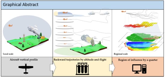
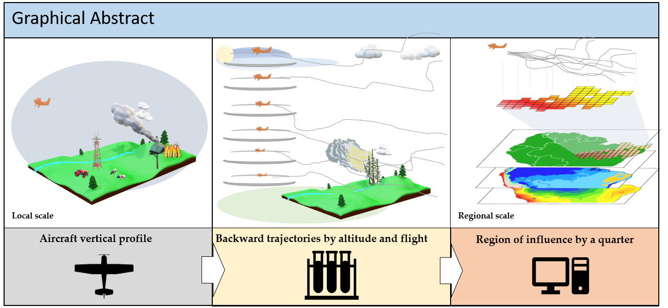
Determination of Region of Influence Obtained by Aircraft Vertical Profiles Using the Density of Trajectories from the HYSPLIT Model

 ,
,  ,
,  , ,
, ,  , ,
, ,  ,
,
Abstract
:
1. Introduction
2. Experiments
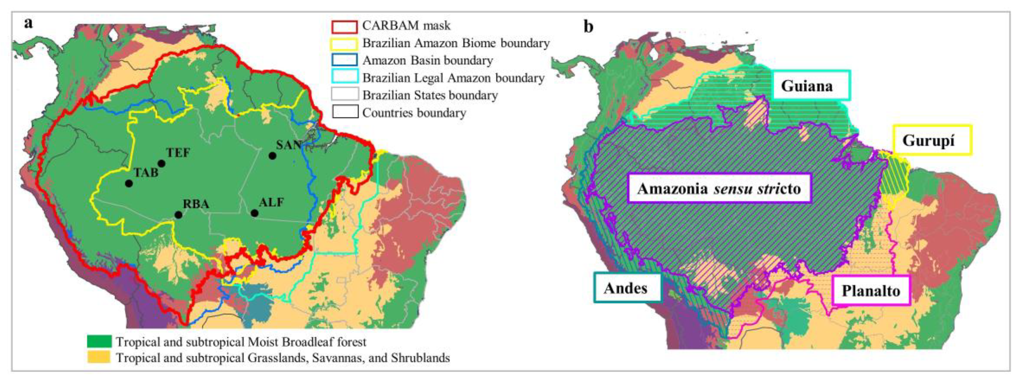
2.1. Amazon Mask
Description of CARBAM Flight Collection Sites
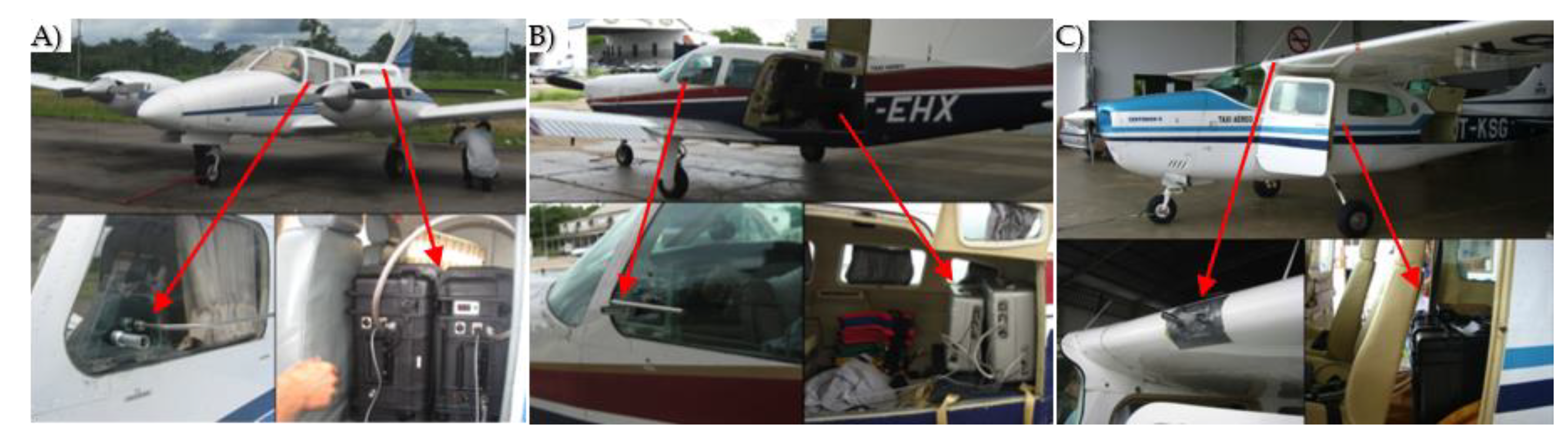
2.2. Aircraft Vertical Profile Air Sampling
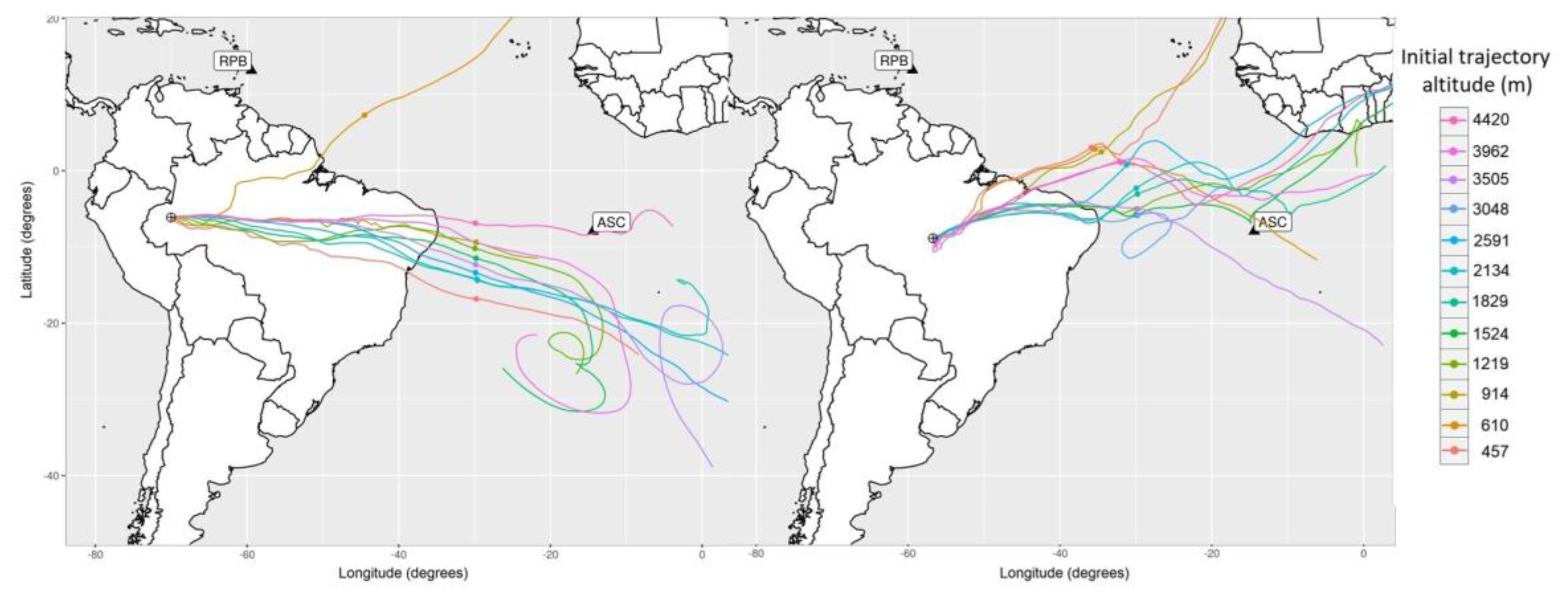
2.3. The HYSPLIT Model
2.4. Region of Influence
The Relative Area inside Amazon
3. Results
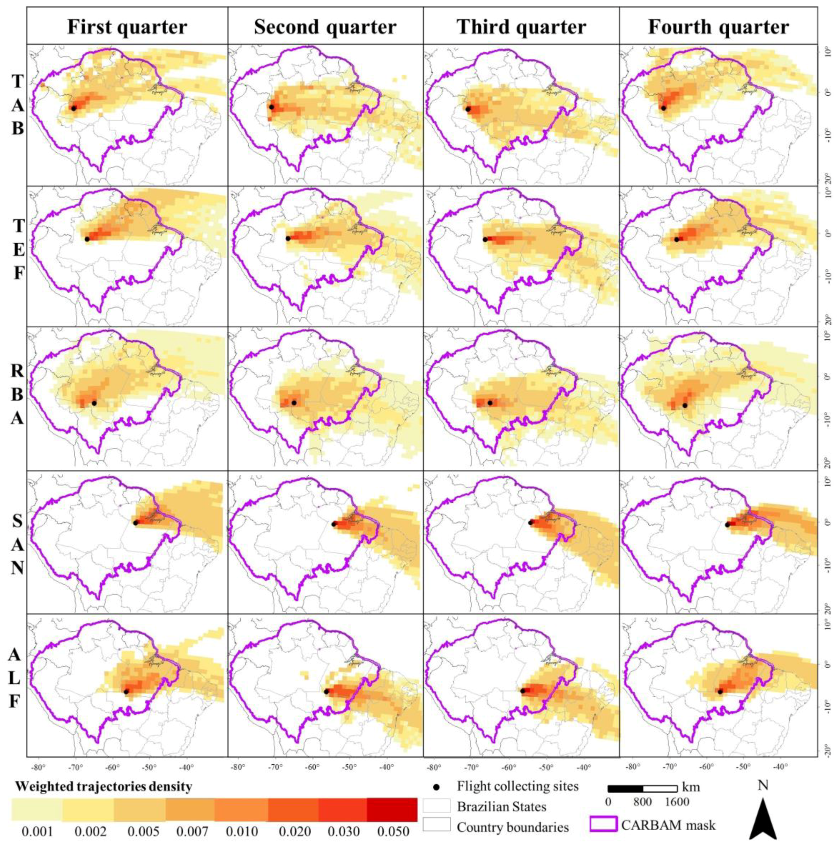
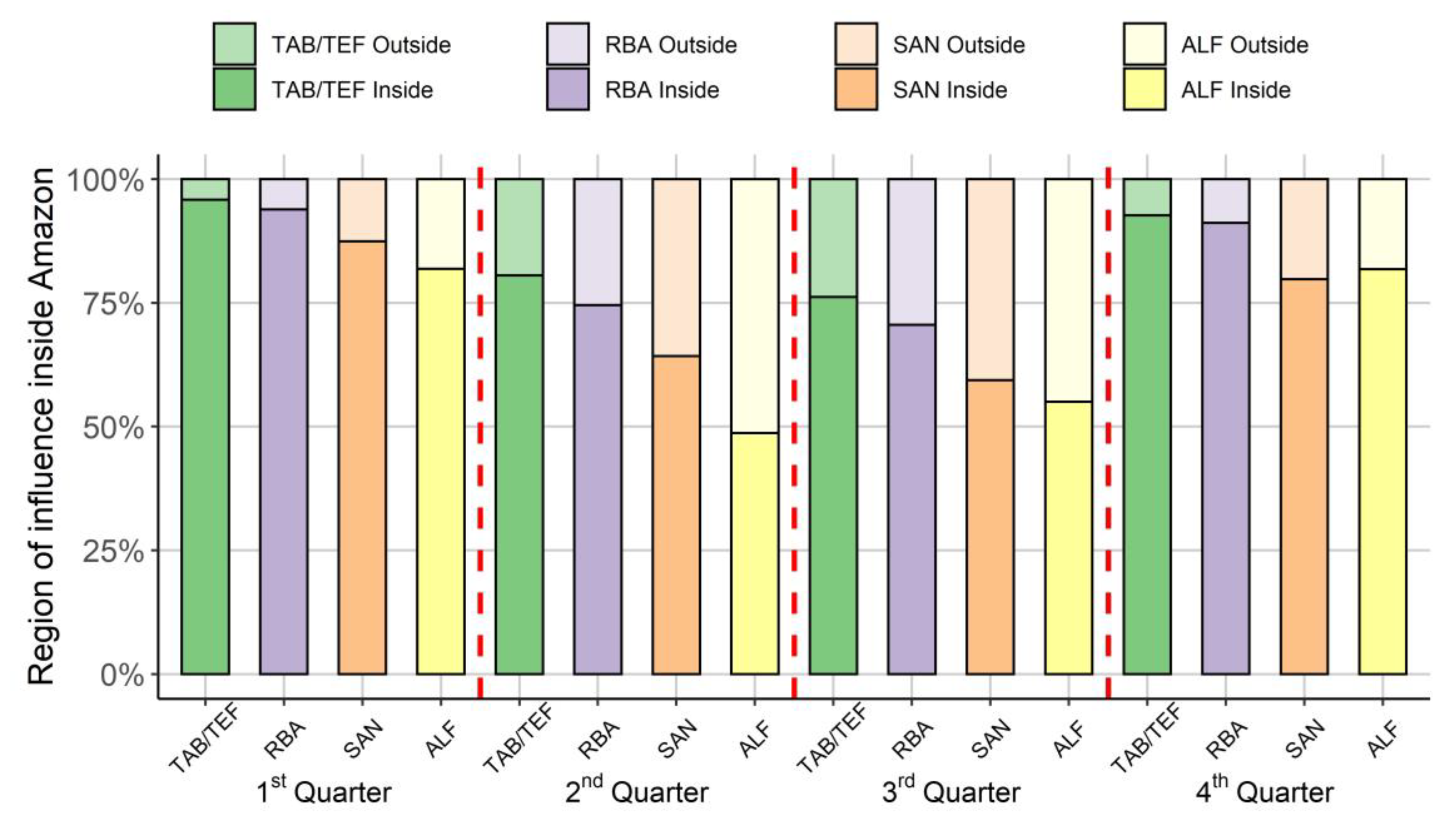
3.1. Quarterly Patterns of the Regions of Influence
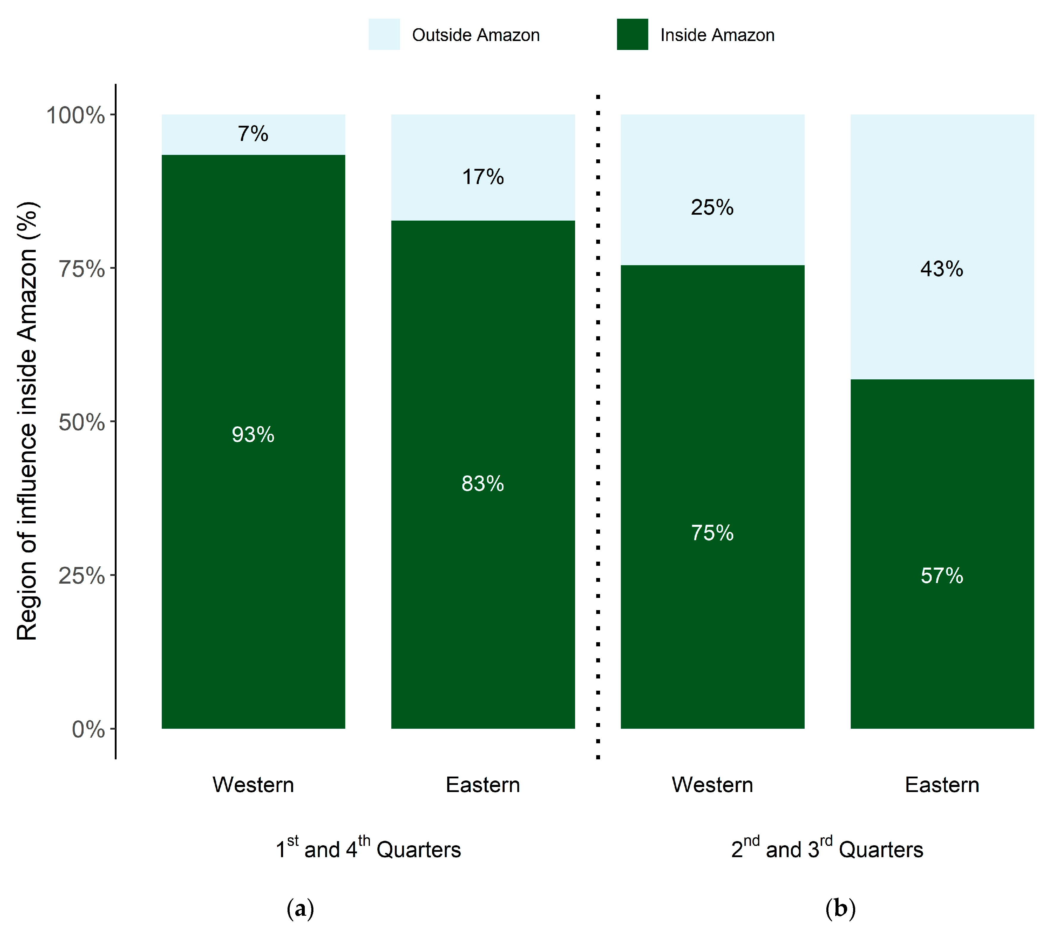
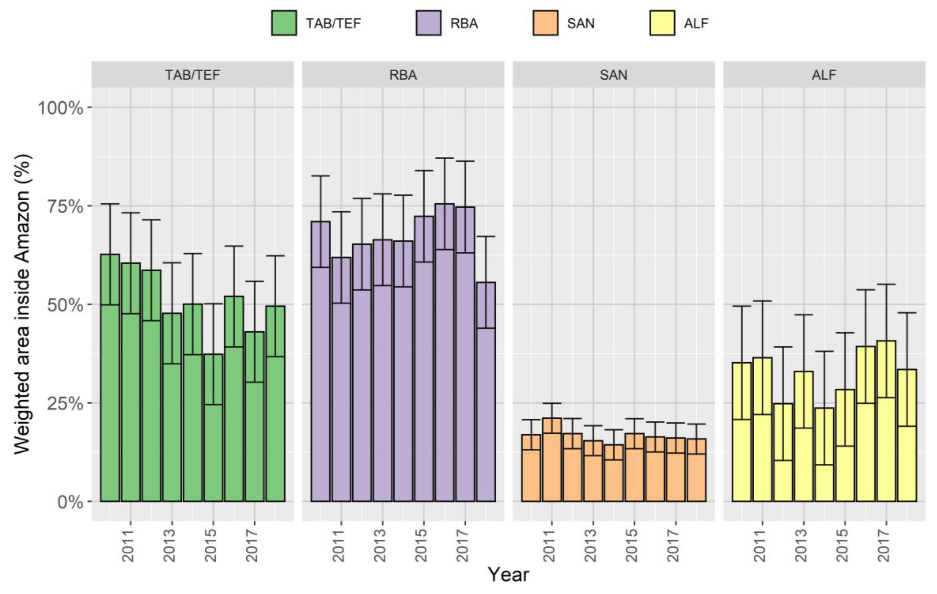
3.2. Contribution of Regions of Influence inside Amazonia
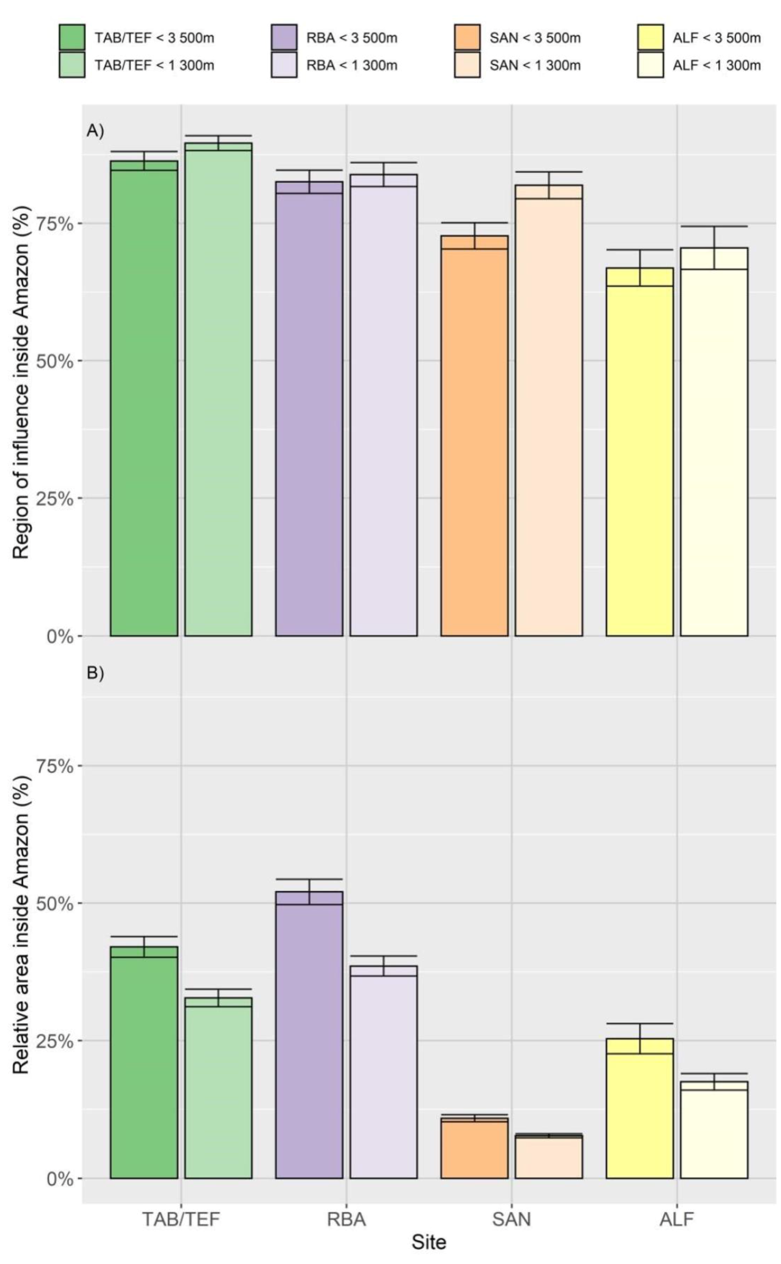
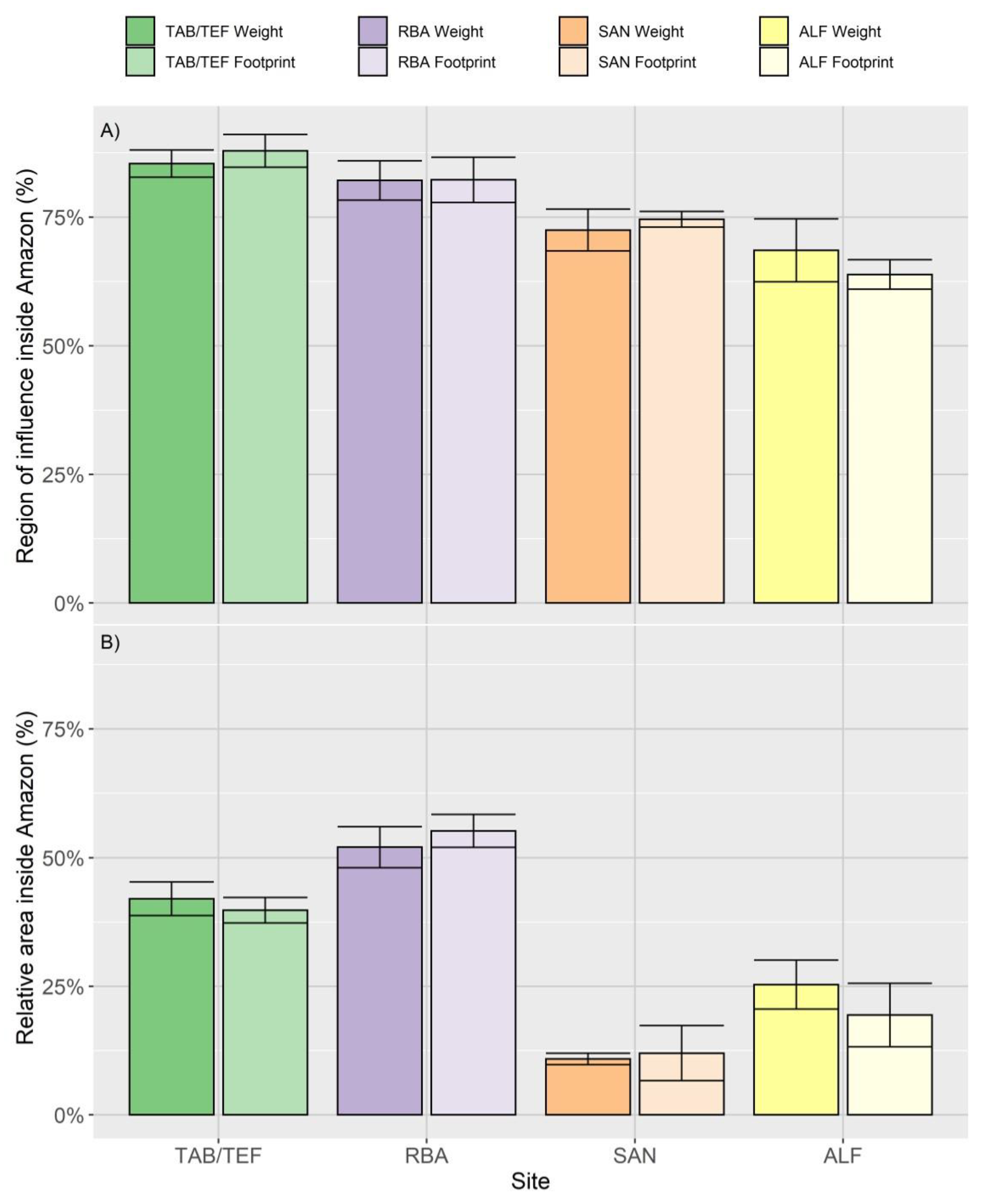
3.3. Representativeness of the Region of Influence in the Amazon
4. Discussion
4.1. What Is the Influence of Spatiotemporal Resolution on the Aggregation of the Results?
4.2. Limitations of the Method
4.3. What Are the Implications for Generalizations of GHG Fluxes at Regional Scales?
5. Conclusions
Supplementary Materials
Author Contributions
Funding
Acknowledgments
Conflicts of Interest
References
- Ciais, P.; Sabine, C.; Bala, G.; Bopp, L.; Brovkin, V.; Canadell, J.; Chhabra, A.; DeFries, R.; Galloway, J.; Heimann, M.; et al. The physical science basis. Contribution of working group I to the fifth assessment report of the intergovernmental panel on climate change. Chang. IPCC Clim. 2013, 1, 465–570. [Google Scholar]
- Friedlingstein, P.; Cox, P.; Betts, R.; Bopp, L.; von Bloh, W.; Brovkin, V.; Cadule, P.; Doney, S.; Eby, M.; Fung, I.; et al. Climate-carbon cycle feedback analysis: Results from the C4MIP model intercomparison. J. Clim. 2006, 19, 3337–3353. [Google Scholar] [CrossRef]
- Bloom, A.A.; Williams, M. Constraining ecosystem carbon dynamics in a data-limited world: Integrating ecological “common sense” in a model-data fusion framework. Biogeosciences 2015, 12, 1299–1315. [Google Scholar] [CrossRef] [Green Version]
- van der Laan-Luijkx, I.R.; Krol, M.C.; Gatti, L.V.; Domingues, L.G.; Correia, C.S.C.; Miller, J.B.; Gloor, M.; Leeuwen, T.T.; Kaiser, J.W.; Wiedinmyer, C.; et al. Global Biogeochemical Cycles drought derived with CarbonTracker South America. Glob. Biogeochem. Cycles 2015, 29, 1092–1108. [Google Scholar] [CrossRef] [Green Version]
- Alden, C.B.; Miller, J.B.; Gatti, L.V.; Gloor, M.M.; Guan, K.; Michalak, A.M.; van der Laan-Luijkx, I.T.; Touma, D.; Andrews, A.; Basso, L.S.; et al. Regional atmospheric CO2 inversion reveals seasonal and geographic differences in Amazon net biome exchange. Glob. Chang. Biol. 2016, 22, 3427–3443. [Google Scholar] [CrossRef]
- Baldocchi, D.D.; Hincks, B.B.; Meyers, T.P. Measuring Biosphere-Atmosphere Exchanges of Biologically Related Gases with Micrometeorological Methods. Ecology 1988, 69, 1331–1340. [Google Scholar] [CrossRef]
- Knohl, A.; Baldocchi, D.D. Effects of diffuse radiation on canopy gas exchange processes in a forest ecosystem. J. Geophys. Res. Biogeosci. 2008, 113. [Google Scholar] [CrossRef]
- Desjardins, R.L.; Worth, D.E.; Pattey, E.; VanderZaag, A.; Srinivasan, R.; Mauder, M.; Worthy, D.; Sweeney, C.; Metzger, S. The challenge of reconciling bottom-up agricultural methane emissions inventories with top-down measurements. Agric. For. Meteorol. 2018, 248, 48–59. [Google Scholar] [CrossRef] [Green Version]
- Gurney, K.R.; Law, R.M.; Denning, A.S.; Rayner, P.J.; Baker, D.; Bousquet, P.; Bruhwiler, L.; Chen, Y.-H.; Ciais, P.; Fan, S.; et al. Towards robust regional estimates of CO2 sources and sinks using atmospheric transport models. Nature 2002, 415, 626–630. [Google Scholar] [CrossRef] [Green Version]
- Peters, W.; Jacobson, A.R.; Sweeney, C.; Andrews, A.E.; Conway, T.J.; Masarie, K.; Miller, J.B.; Bruhwiler, L.M.P.; Petron, G.; Hirsch, A.I.; et al. An atmospheric perspective on North American carbon dioxide exchange: CarbonTracker. Proc. Natl. Acad. Sci. USA 2007, 104, 18925–18930. [Google Scholar] [CrossRef] [Green Version]
- Jung, M.; Schwalm, C.; Migliavacca, M.; Walther, S.; Camps-Valls, G.; Koirala, S.; Anthoni, P.; Besnard, S.; Bodesheim, P.; Carvalhais, N.; et al. Scaling carbon fluxes from eddy covariance sites to globe: Synthesis and evaluation of the FLUXCOM approach. Biogeosciences 2020, 17, 1343–1365. [Google Scholar] [CrossRef] [Green Version]
- Gatti, L.V.; Gloor, M.; Miller, J.B.; Doughty, C.E.; Malhi, Y.; Domingues, L.G.; Basso, L.S.; Martinewski, A.; Correia, C.S.C.; Borges, V.F.; et al. Drought sensitivity of Amazonian carbon balance revealed by atmospheric measurements. Nature 2014, 506, 76–80. [Google Scholar] [CrossRef] [PubMed]
- Basso, L.S.; Gatti, L.V.; Gloor, M.; Miller, J.B.; Domingues, L.G.; Correia, C.S.C.; Borges, V.F. Seasonality and interannual variability of CH 4 fluxes from the eastern Amazon Basin inferred from atmospheric mole fraction profiles. J. Geophys. Res. Atmos. 2016, 121, 168–184. [Google Scholar] [CrossRef] [PubMed]
- Kondo, M.; Ichii, K.; Takagi, H.; Sasakawa, M. Comparison of the data-driven top-down and bottom-up global terrestrial CO2 exchanges: GOSAT CO2 inversion and empirical eddy flux upscaling. J. Geophys. Res. Biogeosci. 2015, 120, 1226–1245. [Google Scholar] [CrossRef]
- Basu, S.; Guerlet, S.; Butz, A.; Houweling, S.; Hasekamp, O.; Aben, I.; Krummel, P.; Steele, P.; Langenfelds, R.; Torn, M.; et al. Global CO2 fluxes estimated from GOSAT retrievals of total column CO2. Atmos. Chem. Phys. 2013, 13, 8695–8717. [Google Scholar] [CrossRef] [Green Version]
- Lin, J.C.; Gerbig, C.; Wofsy, S.C.; Andrews, A.E.; Daube, B.C.; Davis, K.J.; Grainger, C.A. A near-field tool for simulating the upstream influence of atmospheric observations: The Stochastic Time-Inverted Lagrangian Transport (STILT) model. J. Geophys. Res. Atmos. 2003, 108. [Google Scholar] [CrossRef] [Green Version]
- Stohl, A.; Hittenberger, M.; Wotawa, G. Validation of the Lagrangian particle dispersion model FLEXPART against large-scale tracer experiment data. Atmos. Environ. 1998, 32, 4245–4264. [Google Scholar] [CrossRef]
- Gerbig, C.; Lin, J.C.; Wofsy, S.C.; Daube, B.C.; Andrews, A.E.; Stephens, B.B.; Bakwin, P.S.; Grainger, C.A. Toward constraining regional-scale fluxes of CO2 with atmospheric observations over a continent: 2. Analysis of COBRA data using a receptor-oriented framework. J. Geophys. Res. Atmos. 2003, 108. [Google Scholar] [CrossRef] [Green Version]
- Hu, L.; Andrews, A.E.; Thoning, K.W.; Sweeney, C.; Miller, J.B.; Michalak, A.M.; Dlugokencky, E.; Tans, P.P.; Shiga, Y.P.; Mountain, M.; et al. Enhanced North American carbon uptake associated with El Niño. Sci. Adv. 2019, 5, 1–11. [Google Scholar] [CrossRef] [Green Version]
- Martins, D.K.; Sweeney, C.; Stirm, B.H.; Shepson, P.B. Regional surface flux of CO2 inferred from changes in the advected CO2 column density. Agric. For. Meteorol. 2009, 149, 1674–1685. [Google Scholar] [CrossRef]
- Draxler, R.R.; Hess, G.D. An overview of the HYSPLIT_4 modelling system for trajectories, dispersion and deposition. Aust. Meteorol. Mag. 1998, 47, 295–308. [Google Scholar]
- Eva, H.D.; Huber, O.; Achard, F.; Balslev, H.; Beck, S.; Behling, H.; Belward, A.S.; Beuchle, R.; Cleef, A.M.; Colchester, M.; et al. A Proposal for Defining the Geographical Boundaries of Amazonia; Synthesis of the Results from an Expert Consultation Workshop Organized by the European Commission in Collaboration with the Amazon Cooperation Treaty Organization—JRC Ispra, 7–8 June 2005; EC: Luxembourg, 2005; ISBN 9279000128. [Google Scholar]
- Olson, D.M.; Dinerstein, E.; Wikramanayake, E.D.; Burgess, N.D.; Powell, G.V.N.; Underwood, E.C.; D’amico, J.A.; Itoua, I.; Strand, H.E.; Morrison, J.C.; et al. Terrestrial Ecoregions of the World: A New Map of Life on Earth. Bioscience 2001, 51, 933. [Google Scholar] [CrossRef]
- FAPESP—São Paulo Research Foundation. CARBAM Project: The Amazon Carbon Balance Long-Term Study. Available online: https://bv.fapesp.br/en/auxilios/97938/interannual-variation-of-amazon-basin-greenhouse-gas-balances-and-their-controls-in-a-warming-and-in/ (accessed on 18 June 2020).
- Gatti, L.V.; Miller, J.B.; D’amelio, M.T. aS.; Martinewski, A.; Basso, L.S.; Gloor, M.E.; Wofsy, S.; Tans, P. Vertical profiles of CO2 above eastern Amazonia suggest a net carbon flux to the atmosphere and balanced biosphere between 2000 and 2009. Tellus B Chem. Phys. Meteorol. 2010, 62, 581–594. [Google Scholar] [CrossRef] [Green Version]
- Coe, M.T.; Macedo, M.N.; Brando, P.M.; Lefebvre, P.; Panday, P.; Silvério, D. The Hydrology and Energy Balance of the Amazon Basin. In Ecological Studies; Nagy, L., Forsberg, B.R., Artaxo, P., Eds.; Springer: Berlin/Heidelberg, Germany, 2016; Volume 227, pp. 139–148. ISBN 978-3-662-49900-9. [Google Scholar]
- Climate Data. Climate Model with 220 mi Points Interpolated in 30 Arc Seconds Spatial Resolution. Data from 1982 to 2012. Available online: https://pt.climate-data.org/ (accessed on 17 May 2020).
- INPE. Amazon Deforestation Monitoring Project (PRODES). São José dos Campos, SP, Brazil. 2019. Available online: http://www.obt.inpe.br/OBT/assuntos/programas/amazonia/prodes (accessed on 18 May 2020).
- Tejada, G.; Dalla-Nora, E.; Cordoba, D.; Lafortezza, R.; Ovando, A.; Assis, T.; Aguiar, A.P. Deforestation scenarios for the Bolivian lowlands. Environ. Res. 2016, 144, 49–63. [Google Scholar] [CrossRef] [PubMed]
- Ometto, J.P.; Sousa-Neto, E.R.; Tejada, G. Land Use, Land Cover and Land Use Change in the Brazilian Amazon (1960–2013). In Ecological Studies; Springer: Berlin, Germany, 2016; Volume 227, pp. 369–383. ISBN 978-3-662-49900-9. [Google Scholar]
- Mapbiomas. Proyecto MapBiomas Amazonía—Colección [1.0] de los mapas anuales de cobertura y uso del suelo. Available online: http://amazonia.mapbiomas.org (accessed on 18 April 2019).
- Miller, J.B.; Gatti, L.V.; D’Amelio, M.T.S.; Crotwell, A.M.; Dlugokencky, E.J.; Bakwin, P.; Artaxo, P.; Tans, P.P. Airborne measurements indicate large methane emissions from the eastern Amazon basin. Geophys. Res. Lett. 2007, 34, L10809. [Google Scholar] [CrossRef] [Green Version]
- Domingues, L.G. As emissões de carbono provenientes da queima de biomassa e os fatores que a influenciam na Amazônia, 2019. Ph.D. Thesis, Ciências na Área de Tecnologia Nuclear, Instituto de Pesquisas Energéticas e Nucleares, Universidade de São Paulo, São Paulo, Brazil, 23 September 2019. [Google Scholar]
- Stein, A.F.; Draxler, R.R.; Rolph, G.D.; Stunder, B.J.B.; Cohen, M.D.; Ngan, F. NOAA’s HYSPLIT Atmospheric Transport and Dispersion Modeling System. Bull. Am. Meteorol. Soc. 2015, 96, 2059–2077. [Google Scholar] [CrossRef]
- Draxler, R.R.; Rolph, G.D. Evaluation of the Transfer Coefficient Matrix (TCM) approach to model the atmospheric radionuclide air concentrations from Fukushima. J. Geophys. Res. Atmos. 2012, 117. [Google Scholar] [CrossRef]
- Pöhlker, C.; Walter, D.; Paulsen, H.; Könemann, T.; Rodríguez-Caballero, E.; Moran-Zuloaga, D.; Brito, J.; Carbone, S.; Degrendele, C.; Després, V.R.; et al. Land cover and its transformation in the backward trajectory footprint region of the Amazon Tall Tower Observatory. Atmos. Chem. Phys. 2019, 19, 8425–8470. [Google Scholar] [CrossRef] [Green Version]
- Rolph, G.; Stein, A.; Stunder, B. Real-time Environmental Applications and Display sYstem: READY. Environ. Model. Softw. 2017, 95, 210–228. [Google Scholar] [CrossRef]
- Gatti Domingues, L.; Vanni Gatti, L.; Aquino, A.; Sánchez, A.; Correia, C.; Gloor, M.; Peters, W.; Miller, J.; Turnbull, J.; Santana, R.; et al. A New Background Method for Greenhouse Gases Flux Calculation Based in Back-Trajectories Over the Amazon. Atmosphere 2020, 11, 734. [Google Scholar] [CrossRef]
- R Development Core Team. R: A Language and Environment for Statistical Computing; R Development Core Team: Vienna, Austria, 2008. [Google Scholar]
- Cavalcanti, I.F.A.; Ferreira, N.J.; Dias, M.A.F.S.; Silva, M.G.A.J. Tempo e clima no Brasil, 1st ed.; Editora Oficina de Textos: Rio de Janeiro, Brazil, 2009; 454p. [Google Scholar]
- Marengo, J.A.; Souza, C.M.; Thonicke, K.; Burton, C.; Halladay, K.; Betts, R.A.; Alves, L.M.; Soares, W.R. Changes in Climate and Land Use Over the Amazon Region: Current and Future Variability and Trends. Front. Earth Sci. 2018, 6, 228. [Google Scholar] [CrossRef]
- Figueroa, S.N.; Nobre, C.A. Precipitation distribution over central and western tropical South America. Climanálise 1990, 5, 36–45. [Google Scholar]
- Fu, R.; Arias, P.A.; Wang, H. The Connection between the North and South American Monsoons. Springer Clim. 2016, 187–206. [Google Scholar]
- Nobre, C.A.; Obregón, G.O.; Marengo, J.A. Características do Clima Amazônico: Aspectos Principais. Amaz. Glob. Chang. 2009, 149–162. [Google Scholar]
- Marengo, J.A. Interannual variability of deep convection over the tropical South American sector as deduced from ISCCP C2 data. Int. J. Climatol. 1995, 15, 995–1010. [Google Scholar] [CrossRef]
- Salati, E.; Marques, J. Climatology of the Amazon region. In The Amazon—Limnology and Landscape Ecology of a Mighty Tropical River and Its Basin; Sioli, H., Ed.; Dr. W. Junk Publishers: Devon, UK, 1984; pp. 85–126. [Google Scholar]
- NOAA—National Oceanic and Atmospheric Administration. ASL—Air Resources Laboratory. Hysplit. Available online: https://www.arl.noaa.gov/hysplit/hysplit-frequently-asked-questions-faqs/faq-hg11/ (accessed on 18 June 2020).
- Brioude, J.; Angevine, W.M.; McKeen, S.A.; Hsie, E.-Y. Numerical uncertainty at mesoscale in a Lagrangian model in complex terrain. Geosci. Model Dev. 2012, 5, 1127–1136. [Google Scholar] [CrossRef] [Green Version]
- Oliveira, M.I.; Acevedo, O.C.; Sörgel, M.; Nascimento, E.L.; Manzi, A.O.; Oliveira, P.E.S.; Brondani, D.V.; Tsokankunku, A.; Andreae, M.O. Planetary boundary layer evolution over the Amazon rainforest in episodes of deep moist convection at the Amazon Tall Tower Observatory. Atmos. Chem. Phys. 2020, 20, 15–27. [Google Scholar] [CrossRef] [Green Version]
- van der Laan-Luijkx, I.T.; van der Velde, I.R.; Krol, M.C.; Gatti, L.V.; Domingues, L.G.; Correia, C.S.C.; Miller, J.B.; Gloor, M.; van Leeuwen, T.T.; Kaiser, J.W.; et al. Response of the Amazon carbon balance to the 2010 drought derived with CarbonTracker South America. Glob. Biogeochem. Cycles 2015, 29, 1092–1108. [Google Scholar] [CrossRef] [Green Version]


| Number of Flights (Number of Simulated Flights) | ||||
|---|---|---|---|---|
| Year | TAB/TEF | RBA | SAN | ALF |
| 2010 | 19(5) | 19(5) | 19(5) | 19(5) |
| 2011 | 14(10) | 17(7) | 22(2) | 18(6) |
| 2012 | 9(15) | 22(2) | 24(0) | 24(0) |
| 2013 | 8(16) | 17(7) | 23(1) | 21(3) |
| 2014 | 16(8) | 13(12) | 16(8) | 17(7) |
| 2015 | 4(20) | 11(14) | 6(18) | 5(19) |
| 2016 | 0(24) | 20(4) | 0(24) | 20(4) |
| 2017 | 14(10) | 21(3) | 17(7) | 24(0) |
| 2018 | 13(11) | 20(4) | 18(6) | 24(0) |
| Total | 97(119) | 160(56) | 145(71) | 172(44) |
| TAB/TEF | RBA | SAN | ALF | |||||
|---|---|---|---|---|---|---|---|---|
| Year/ | Area | Area | Area | % | Area | % | Area | % |
| Quarter | (km2) | (km2) | (km2) | Amz | (km2) | Amz | (km2) | Amz |
| 2010 | 3,759,861 | 3,759,861 | 3,821,599 | 52.7% | 645,165 | 8.9% | 1,876,844 | 25.9% |
| 1st | 4,753,849 | 4,753,849 | 4,309,332 | 59.4% | 642,078 | 8.8% | 2,111,450 | 29.1% |
| 2nd | 2,741,179 | 2,741,179 | 3,321,521 | 45.8% | 617,383 | 8.5% | 1,210,068 | 16.7% |
| 3rd | 4,136,467 | 4,136,467 | 3,333,864 | 45.9% | 814,944 | 11.2% | 1,197,722 | 16.5% |
| 4th | 3,407,951 | 3,407,951 | 4,321,678 | 59.6% | 506,254 | 7.0% | 2,988,134 | 41.2% |
| 2011 | 3,728,991 | 3,728,991 | 3,528,342 | 48.6% | 1,083,506 | 14.9% | 2,031,188 | 28.0% |
| 1st | 3,815,425 | 3,815,425 | 4,358,723 | 60.1% | 1,518,762 | 20.9% | 3,593,166 | 49.5% |
| 2nd | 4,062,381 | 4,062,381 | 2,333,709 | 32.2% | 679,120 | 9.4% | 1,123,635 | 15.5% |
| 3rd | 3,728,989 | 3,728,989 | 3,099,259 | 42.7% | 938,422 | 12.9% | 950,770 | 13.1% |
| 4th | 3,309,170 | 3,309,170 | 4,321,677 | 59.6% | 1,197,722 | 16.5% | 2,457,182 | 33.9% |
| 2012 | 3,636,385 | 3,636,385 | 3,908,033 | 53.9% | 814,945 | 11.2% | 1,188,462 | 16.4% |
| 1st | 3,568,471 | 3,568,471 | 4,185,853 | 57.7% | 814,945 | 11.2% | 1,654,587 | 22.8% |
| 2nd | 3,840,121 | 3,840,121 | 3,444,995 | 47.5% | 617,382 | 8.5% | 728,511 | 10.0% |
| 3rd | 3,432,648 | 3,432,648 | 3,444,997 | 47.5% | 716,165 | 9.9% | 617,382 | 8.5% |
| 4th | 3,704,297 | 3,704,297 | 4,556,285 | 62.8% | 1,111,289 | 15.3% | 1,753,367 | 24.2% |
| 2013 | 2,898,612 | 2,898,612 | 3,648,732 | 50.3% | 830,379 | 11.4% | 2,000,319 | 27.6% |
| 1st | 1,926,235 | 1,926,235 | 4,556,283 | 62.8% | 555,645 | 7.7% | 3,074,565 | 42.4% |
| 2nd | 3,593,166 | 3,593,166 | 3,580,818 | 49.3% | 629,730 | 8.7% | 765,554 | 10.6% |
| 3rd | 3,296,825 | 3,296,825 | 2,271,968 | 31.3% | 716,164 | 9.9% | 1,148,331 | 15.8% |
| 4th | 2,778,223 | 2,778,223 | 4,185,857 | 57.7% | 1,419,979 | 19.6% | 3,012,827 | 41.5% |
| 2014 | 2,858,482 | 2,858,482 | 3,704,298 | 51.0% | 691,468 | 9.5% | 1,176,114 | 16.2% |
| 1st | 2,062,059 | 2,062,059 | 3,827,774 | 52.8% | 629,730 | 8.7% | 1,666,932 | 23.0% |
| 2nd | 2,914,045 | 2,914,045 | 3,235,087 | 44.6% | 753,206 | 10.4% | 765,556 | 10.6% |
| 3rd | 2,531,270 | 2,531,270 | 2,975,787 | 41.0% | 691,468 | 9.5% | 938,422 | 12.9% |
| 4th | 3,926,554 | 3,926,554 | 4,778,544 | 65.9% | 691,469 | 9.5% | 1,333,547 | 18.4% |
| 2015 | 2,228,751 | 2,228,751 | 4,065,463 | 56.0% | 839,640 | 11.6% | 1,577,413 | 21.7% |
| 1st | 2,531,269 | 2,531,269 | 4,420,460 | 60.9% | 1,444,676 | 19.9% | 2,901,700 | 40.0% |
| 2nd | 2,309,010 | 2,309,010 | 3,840,117 | 52.9% | 642,078 | 8.8% | 1,160,679 | 16.0% |
| 3rd | 1,827,453 | 1,827,453 | 3,370,906 | 46.5% | 654,425 | 9.0% | 1,222,417 | 16.8% |
| 4th | 2,247,272 | 2,247,272 | 4,630,368 | 63.8% | 617,382 | 8.5% | 1,024,856 | 14.1% |
| 2016 | 2,985,046 | 2,985,046 | 3,870,988 | 53.3% | 743,946 | 10.3% | 2,278,142 | 31.4% |
| 1st | 2,259,621 | 2,259,621 | 3,938,900 | 54.3% | 629,730 | 8.7% | 2,951,091 | 40.7% |
| 2nd | 2,494,227 | 2,494,227 | 2,370,748 | 32.7% | 802,599 | 11.1% | 814,946 | 11.2% |
| 3rd | 3,012,828 | 3,012,828 | 3,383,256 | 46.6% | 814,945 | 11.2% | 1,815,103 | 25.0% |
| 4th | 4,173,507 | 4,173,507 | 5,791,048 | 79.8% | 728,512 | 10.0% | 3,531,428 | 48.7% |
| 2017 | 2,583,747 | 2,583,747 | 4,173,508 | 57.5% | 731,598 | 10.1% | 2,420,141 | 33.4% |
| 1st | 2,247,273 | 2,247,273 | 4,753,848 | 65.5% | 839,640 | 11.6% | 4,704,457 | 64.8% |
| 2nd | 3,037,521 | 3,037,521 | 3,370,911 | 46.5% | 765,554 | 10.6% | 950,770 | 13.1% |
| 3rd | 2,617,704 | 2,617,704 | 2,901,697 | 40.0% | 654,425 | 9.0% | 1,024,856 | 14.1% |
| 4th | 2,432,489 | 2,432,489 | 5,667,574 | 78.1% | 666,773 | 9.2% | 3,000,482 | 41.3% |
| 2018 | 2,775,135 | 2,775,135 | 3,272,130 | 45.1% | 722,338 | 10.0% | 2,000,320 | 27.6% |
| 1st | 2,531,268 | 2,531,268 | 3,815,424 | 52.6% | 889,031 | 12.3% | 3,667,254 | 50.5% |
| 2nd | 3,074,565 | 3,074,565 | 4,519,245 | 62.3% | 790,249 | 10.9% | 1,580,500 | 21.8% |
| 3rd | 3,111,606 | 3,111,606 | 1,889,192 | 26.0% | 654,426 | 9.0% | 913,727 | 12.6% |
| 4th | 2,383,098 | 2,383,098 | 2,864,657 | 39.5% | 555,645 | 7.7% | 1,839,801 | 25.4% |
| Average | 3,050,557 | 3,050,557 | 3,777,010 | 52.1% | 789,221 | 10.9% | 1,838,772 | 25.3% |
© 2020 by the authors. Licensee MDPI, Basel, Switzerland. This article is an open access article distributed under the terms and conditions of the Creative Commons Attribution (CC BY) license (http://creativecommons.org/licenses/by/4.0/).
Share and Cite
Cassol, H.L.G.; Domingues, L.G.; Sanchez, A.H.; Basso, L.S.; Marani, L.; Tejada, G.; Arai, E.; Correia, C.; Alden, C.B.; Miller, J.B.; et al. Determination of Region of Influence Obtained by Aircraft Vertical Profiles Using the Density of Trajectories from the HYSPLIT Model. Atmosphere 2020, 11, 1073. https://doi.org/10.3390/atmos11101073
Cassol HLG, Domingues LG, Sanchez AH, Basso LS, Marani L, Tejada G, Arai E, Correia C, Alden CB, Miller JB, et al. Determination of Region of Influence Obtained by Aircraft Vertical Profiles Using the Density of Trajectories from the HYSPLIT Model. Atmosphere. 2020; 11(10):1073. https://doi.org/10.3390/atmos11101073
Chicago/Turabian StyleCassol, Henrique L. G., Lucas G. Domingues, Alber H. Sanchez, Luana S. Basso, Luciano Marani, Graciela Tejada, Egidio Arai, Caio Correia, Caroline B. Alden, John B. Miller, and et al. 2020. "Determination of Region of Influence Obtained by Aircraft Vertical Profiles Using the Density of Trajectories from the HYSPLIT Model" Atmosphere 11, no. 10: 1073. https://doi.org/10.3390/atmos11101073