Multi-Physics Modeling of Steel Ingot Melting by Electric Arc Plasma and its Application to Electric Arc Furnace

Introduction

Arc melting is an electro-thermal processing method that utilizes electrical energy to generate electric arc plasma to melt down the target material. The arc melting of metal and alloy is a critical subset of such applications (Backer and Szekely, 1987). Compared with other melting approaches, the electric arc plasma is capable of efficiently melting solid material with a high melting point or hardness without introducing impurity, which produces high-quality liquid metal or alloy meeting the different requirements for product performance (Sames, 2015). This technology is therefore a widely-used melting method in modern material manufacturing.

Generally, using the electric arc for the solid material melting involves the ionization of the gas molecules, the generation of the high-temperature arc, the interaction between the arc and the exposed solid surface, the heating and melting of the solid material, and the impingement and stirring of the arc to the molten liquid. Thus, the system includes the gas phase, liquid phase, solid phase, and arc plasma, with the volume fraction of each phase constantly changing during the entire process (Apelian et al., 1983). Due to the complexity of such a multi-physical process, some models (Dowden and Kapadia, 1994; Yin et al., 2007) only focused on the electric arc plasma region and considered the top surface of the solid instead of the entire solid region so that the arc heat transfer characteristics can be studied by analyzing the heat flux on that surface. Although those models provided a good basis for the simulation in the arc region, the solid heating and melting behavior cannot be predicted. In contrast, some other studies (Lago et al., 2004; Tanaka et al., 2004; Li et al., 2017) simulated the heating process of the solid material but ignoring the phase changing or liquid flow. Meanwhile, part of models (Wu et al., 2009; Zhang et al., 2011) introduced the pressure and thermal intensity generated by the electric arc plasma through specific boundary conditions to achieve the consideration of the arc. Thus, the model only included the solid region and the electric arc plasma itself was ignored. These studies provided compromise solutions to simulate the arc melting, but the complete numerical prediction of such a process has not been achieved in essence. Only a few studies (Jian and Wu, 2015; Pan et al., 2016) considered both the electric arc and the dynamic melting process at the same time, but the models focus on the local melting behavior in a small region of the workpiece, like the keyhole plasma arc welding. As for the study of the melting process of full-scale solid materials, there is still a lack of corresponding numerical prediction and analysis.

In fact, the arc plasma, the solid phase, and the liquid phase occurring in the system will continuously interact and affect each other throughout the melting process of entire solid material. Moreover, the flow characteristics of molten liquid under high-temperature and high-pressure conditions further change the heat transfer mechanism and microstructure of the solid material, thereby leading to different surface deformation and melting behavior, which should not be ignored. Thus, it is necessary to develop a fully-described mathematical arc melting model to simulate both the electric arc plasma and the solid melting and dynamically predict the states of each phase in the system, which helps to clearly understand the complete physical process and the numerical modeling methodology. Furthermore, it is also of great significance to provide practical guidance of efficiently preparing high-quality molten liquid in the future.

To sum up, the main purpose of this paper is to establish a self-consistent mathematical model coupling the electric arc plasma, solid melting, and liquid flow together to simulate the entire solid material melting using the electric arc. The present study focuses on modeling the steel ingot melting, which will be helpful in investigating the electric arc furnace (EAF) scrap melting in the future. The stationary direct current (DC) electric arc modeling and the arc-solid steel interface heat transfer and force interaction modeling were validated respectively against the experimental data to prove the accuracy of the model. The analysis was first conducted on the DC electric arc behavioral characteristics with varying arc length generated by the moving electrode. Afterward, the model was utilized to dynamically predict the entire steel ingot melting using the electric arc, which includes the continuous phase changing of solid steel, the surface deformation of steel ingot, and the close interaction between phases. The study further attempted to evaluate the effects of the initial arc length on the melting efficiency and tried to provide useful guidance for industrial manufacturing. In particular, the model was also implemented to simulate the steel ingot melting with the dynamic electrode movement and made the corresponding comparison to the model without the electrode movement. The study further discussed the feasibility of simulating the EAF scrap melting and proposed a potential method to apply the current model in such a simulation. Preliminary simulation results of the scrap melting in the lab-scale furnace using this potential method were also presented.

Mathematical Model

Problem Description and Simulation Domain

The solid steel ingot is melted in the apparatus shown in Figure 1A. The electrode is inserted from the top of the apparatus to generate a DC electric arc at the electrode tip, melting the steel ingot from top to bottom. The molten liquid steel will flow down the surface of the steel ingot and accumulate at the bottom of the crucible. The apparatus is allowed to connect with the outside atmosphere, and the working gas can be supplemented or escaped through the electrode hole on the top of the apparatus. There is a heat insulation layer around the crucible to prevent heat loss and enhance the melting efficiency. Both the crucible and the steel ingot are cylindrical, and the diameter (W) and height (H) of the inner crucible are 0.04 and 0.03 m, respectively, while the diameter (w) and height (h) of the steel ingot are 0.02 and 0.015 m, respectively. The electrode with the diameter (d) of 0.00454 m can move up and down on its axis as needed. The arc length (l) is originally set to be 0.01 m. Figure 1B shows the simulation domain considered in the present study, which only includes the inner profile of the electrode and the crucible. Due to the axial symmetry of the current physical problem, only half of the geometry in Figure 1B is adopted, and the entire simulation is solved based on the cylindrical coordinate system (r, x) whose origin is located at the center of the electrode tip. The structured mesh has applied to the entire simulation domain, whose total cell number is 454,000 determined after the mesh sensitivity study.

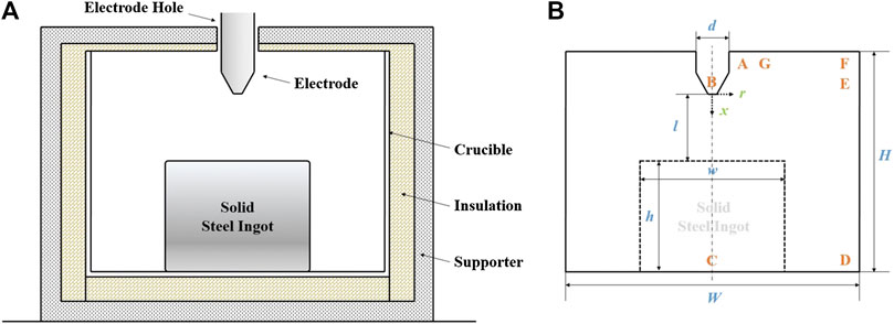
FIGURE 1. (A) Schematic diagram of the lab-scale arc melting furnace. (B) Computational domain for steel ingot melting by the electric arc.

Model Assumptions

In order to conduct the simulation of steel ingot melting by electric arc plasma with the affordable computational time and relatively good accuracy, the following hypotheses are adopted to derive the numerical model in the present study: 1) the arc is considered to be the DC electric arc and is axisymmetric in the 2D configuration (Lago et al., 2004; Tanaka et al., 2004; Li et al., 2017); 2) the arc is optically thin and in local thermodynamic equilibrium (LTE) meaning the temperatures of the electron and heavy particles are very close, which has been proven to be true throughout most of the arc region (Lago et al., 2004; Tanaka et al., 2004; Wu et al., 2009; Zhang et al., 2011; Jian and Wu, 2015; Pan et al., 2016; Li et al., 2017); 3) the effects of heat dissipation due to the viscosity are neglected in all phases (Lowke, 1979); 4) the fluids for both the gas phase and the liquid steel phase are treated as an incompressible Newtonian fluid and the corresponding flows are assumed to be the turbulent flow solved by the standard k-epsilon model (Pan et al., 2016); 5) the Boussinesq’s hypothesis is applied to consider the buoyancy-driven liquid steel flow; 6) the steel vaporization is ignored.

Governing Equations

According to the aforementioned hypotheses, a set of governing equations utilized to describe the system including the gas phase and the steel phase (solid steel and liquid steel) is given as follows. The equation set is based on the volume-of-fluid method, which is capable of capturing the gas-steel free surface deformation and the fluid flow during the melting. Different dynamic and thermal coefficients are applied in different phases, and the equation set is solved in every computational cell of the simulation domain in order to obtain the continuous flow field variables for all phases. The governing equations adopted in the simulation are given below and the flow chart of the comprehensive computational fluid dynamics (CFD) model can be found in Figure 2.

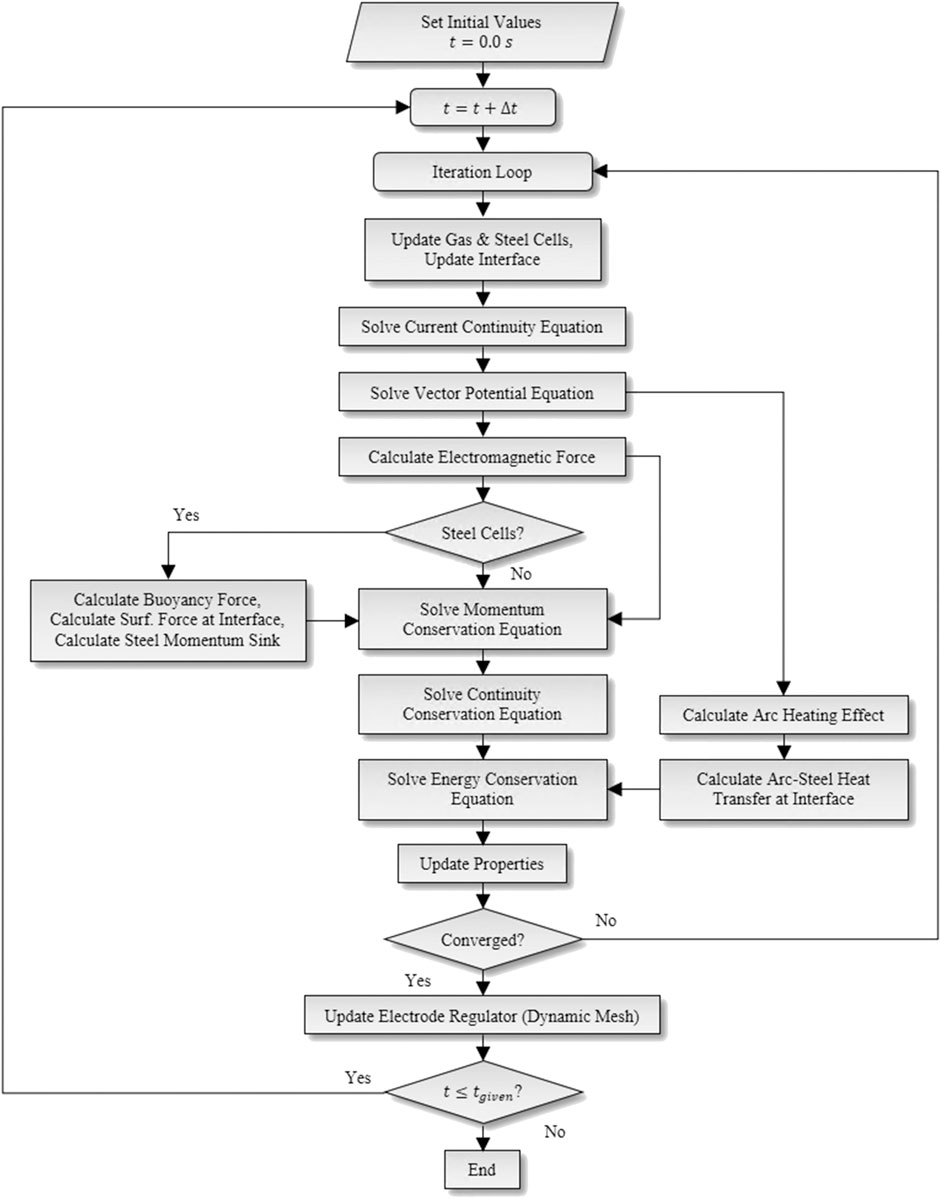
FIGURE 2. Flow chart of the CFD model.

The volume fraction conservation equation can be expressed as:

where ${\alpha }_q$, ${\rho }_q$, and $v_q$ are the volume fraction, the density, and the velocity vector component of phase $q$ (gas or steel), respectively. It should be noted that the sum of the volume fractions in all phases is always unity, i.e., ${\displaystyle {\sum }_{q=1}^n{\alpha }_q=1}$.

The axial and the radial momentum conservation equation are given as:

where $p$ and $\mu$ are the pressure and the viscosity, respectively; $S_{m,b}$ is the additional source term equal to $\rho g\beta \left(T-T_{ref}\right)$, which is for the consideration of the buoyancy force of liquid steel in the anode region; $S_{m,a}$ and $S_{m,sf}$ are another two additional momentum source terms for the arc modeling and the surface force modeling, respectively, which will be illustrated in the later section; $R^{\ast }$ is the coefficient of the momentum sink, which is used to distinguish the anode region. The expression of $R^{\ast }$ can be defined as:

and $C_{mix}$ is the mixture zone constant; $ϵ$ is a coefficient with a small value to prevent zero occurring in the denominator; $\lambda$ is the liquid volume fraction dependent of phase temperature $T$, which can be written as:

and $T_{s,steel}$ and $T_{l,steel}$ are the solidus temperature and the liquidus temperature of the steel phase.

The energy conservation equation can be expressed as:

where $T$ is the temperature; $C_p$ is the specific heat; $k_{eff}$ is the effective thermal conductivity; $S_{e,a}$ and $S_{e,ht}$ are the additional energy source terms, which will be defined in later sections; $S_{e,L}$ is the explicit latent heat term, which is equal to:

where $L$ is the latent heat for the steel ingot melting.

Direct Current Electric Arc Plasma

Another set of equations needs to be solved to obtain the electromagnetic field based on the theory of the magneto hydrodynamics, so that the DC electric arc plasma can be predicted in the model. The calculation of the electrical current density component takes the following forms:

where $\sigma$ is the electrical conductivity of selected working gas; $E$ is the electrical field intensity dependent on the gradient of the electrical potential $V$, which is given by:

The self-induced magnetic field calculation is generally referred to the Biot-Savart formula, however, Ampere’s law can also be employed to roughly measure the azimuthal magnetic induction in an axisymmetric model. The corresponding expressions can be written below:

where $A_x$ and $A_r$ are axial and radial vector potential components, respectively. The determinations of the vector potential components are given in Eqs 13 and 14 listed below.

The current continuity equation is defined as:

And the axial and the radial vector potential equations can be expressed as:

where ${\mu }_0$ is the magnetic permeability in the medium.

By solving the above set of equations, the Lorentz effect and the arc heating effect can be included by two additional source terms in corresponding governing equations, which are written as follows:

where $k_B$ is the Boltzmann constant; $e$ is the elementary electric charge; $S_r$ is the radiation heat loss. The first term on the right-hand side of Eq. 16 represents the heat generated by the Joule’s effect and the second term is referred to the electronic enthalpic flux.

Arc-Steel Ingot Interaction at Interface

Interface Tracking

In order to define a sharp interface between arc plasma region and anode region, a new variable $\eta$ is introduced in the present study:

where $ts$ is the threshold used to distinguish the cell belongs to the anode region or arc plasma region, that is, $\eta$ will be unity if the cell is an anode cell. Therefore, the interface can be represented using the normalized gradient of $\eta$, which is written as:

Heat Transfer at Interface

During the steel ingots arc melting process, there exists a low-temperature sheath on the surface of the arc and steel ingots, where the plasma arc temperature, particle density, and voltage have large gradients, resulting in the plasma not meeting the LTE assumption (Tanaka et al., 2004). The presence of a low-temperature sheath causes the electron temperature to be different from the heavy particle temperature, thus the electron temperature and the heavy particle temperature cannot be defined by a unified temperature value. Meanwhile, such a sheath also has a significant impact on the distribution of the arc current density on the surface of the steel ingot and the heat transfer between the steel ingot and the arc. Therefore, the special treatment of the boundary layer is required in the model. The present study adopted the LTE-diffusion approximation to deal with the above-mentioned low-temperature sheath (Lowke and Tanaka, 2006; Jian and Wu, 2015), and considers the thermal effect of the arc to the steel ingot surface by adding the additional energy source at the interface for each phase (Tashiro et al., 2011). Generally, the heat transfer mechanism from the arc to the steel ingot surface is mainly composed of three parts: the electronic heat, the conduction heat, and the surface radiative heat. Among them, the electronic heat is caused by the steel ingot surface receiving the electrons from the electrode tip and releasing a large amount of heat.

The aforementioned heat transfer mechanism at the interface can be mathematically expressed as (Pan et al., 2016):

where $q_{eh}$ is the electronic heat; $q_{ch}$ is the conduction heat; $q_{rh}$ is the surface radiative heat; $\phi$ is the work function of steel ingot; $T_a$ and $T_s$ are the interface temperature for arc and steel, respectively; $\delta$ is the interface thickness; $\epsilon$ is the emissivity of steel ingot.

Surface Force at Interface

In addition to the gravity, the buoyancy force, and the electromagnetic force, there has extra four surface forces that need to be discussed and further considered about their effect at the interface, which includes the surface tension, the Marangoni shear stress, the arc plasma shear stress and the arc pressure. It should be noted that the last force, i.e. the arc pressure, has already included in the model by solving the corresponding momentum equations described above. Thus only the first three forces need additional treatment.

The surface tension pressure $p_{st}$ at the interface is mainly due to the surface curvature, and its direction is normal to the local free surface, and its value can be calculated by (Brackbill et al., 1992):

where $\gamma$ is the surface tension coefficient; $\overrightarrow{n}$ is the normal vector to the local free surface.

The Marangoni shear stress ${\tau }_{ms}$ is caused by the existence of the temperature gradient, and its direction is tangential to the local free surface, and its value can be estimated by (Fan and Kovacevic, 1999):

where $\overrightarrow{s}$ is the tangential vector to the local free surface.

While the arc plasma shear stress ${\tau }_{as}$ is estimated according to the interface velocity on the arc plasma side and further applied on another side of the interface, i.e. the anode side, and its value can be calculated as follows (Hu and Tsai, 2007):

By adding the above surface forces as a volumetric source term $S_{m,sf}$ to the momentum conservation equation in the appropriate direction, the force interaction at the interface can be predicted as desired.

Electrode Movement

Except for using the stationary electrode position, the present study also includes the moving electrode to generate the electric arc with varying arc length for the steel ingot melting, which is one of the common operations in the arc melting manufacturing. In order to achieve electrode movement in the model, a layering dynamic mesh was used, and the integral form of all conservation equations mentioned above in the dynamic mesh needs to be rewritten as follows for a general scalar $\varphi$ on an arbitrary control volume $V$ whose boundary is moving (ANSYS Inc., 2011):

where $\overrightarrow{u}$ is the flow velocity, ${\overrightarrow{u}}_g$ is the mesh moving velocity, Γ is the diffusion coefficient regarding different conservation equations, and $S_{\varphi }$ is the source term of a general scalar $\varphi$.

By adopting the layering dynamic mesh, the electrode can move up and down on its axis at the assigned proper mesh moving velocity.

Material Properties and Boundary Conditions

The material properties adopted in the present study are listed in Table 1 and they are all referred to the published literature. The properties given in the form of references in the table are temperature-dependent values, which were added to the solver by interpolation for the simulation. In addition, some properties of the steel ingot, such as viscosity, specific heat, thermal conductivity, are also temperature-dependent, which were added in the same way to the solver. Other parameters utilized in the model are all given in Table 2.

TABLE 1. Material properties in the model.

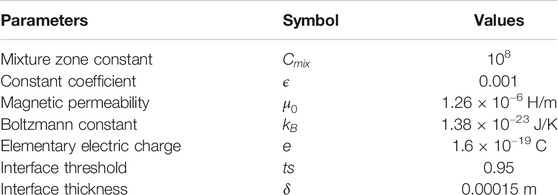
TABLE 2. Other parameters in the model.

The detailed boundary conditions for the simulation domain are indexed in Table 3. It should be noted that a commonly-used free-burning DC arc configuration was adopted in the present study to melt the steel ingot. The operating current is 200 A and the working gas is argon and assumed to be at atmospheric pressure. The corresponding current density distribution expression for this type of arc can be written as follows (Hsu et al., 1983):

where $J_{max}$ is the maximum current density, which can be approximated based on the experimental measurement of the radius of the hottest part (the “white-hot”), and use the following equation to calculate:

where $r_h$ is aforementioned “white hot” radius, and normally takes 0.00051 m for the 200 A arc. And $b$ is a constant, which can be calculated by integrating the current density in radial direction using the expression given below:

where $R_c$ is the arc conduction radius (cut-off radius), and normally takes 0.003 m for the evaluation.

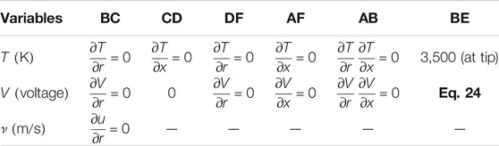
TABLE 3. Boundary conditions for the simulation domain.

Model Validation

Validation of Direct Current Electric Arc Plasma

As the arc is the main heat source for the steel ingot melting, the accuracy of the arc simulation needs to be proven first. Otherwise, the subsequent melting results will be meaningless. The stationary DC electric arc modeling is validated against the temperature measurement of the arc column published in reference. The current validation simulation only includes the electric arc plasma region, i.e. the steel ingot is not considered for the simplification purpose. Figure 3A presents the temperature distribution of the free-burning plasma arc using argon as a working gas. For a 200 A-current arc, the highest temperature located just below the electrode tip can reach up to 22,000 K, while the middle of the arc column maintains a high temperature around 10,000 K. A typical bell shape of the arc plasma can be observed, which is mainly due to the strong impingement and dispersing of the arc plasma jet on the anode surface. Thus, the high temperature gradually spreads along the centerline of the plasma jet and the strong diffusion of the temperature also occurs in the radial direction. The simulation results were compared with the isotherms measured by Hsu et al. (1983). The isotherms range from 11,000 to 21,000 K and the temperature distribution is in a fairly good agreement with the experimental data, whose percentage error is estimated to be less than 5%.

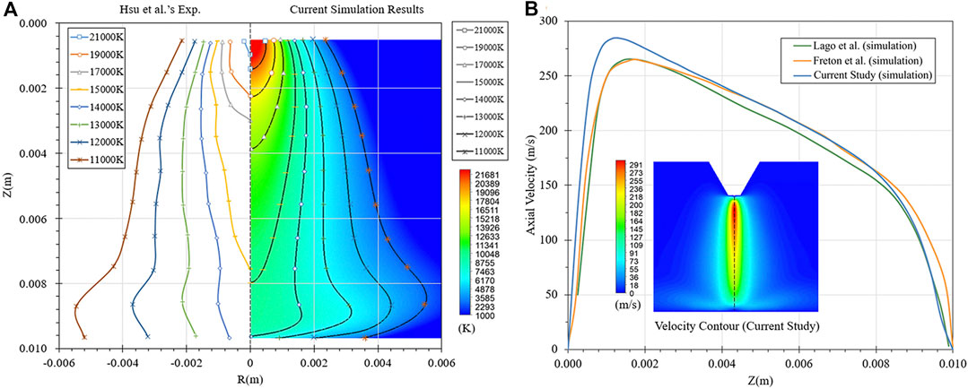
FIGURE 3. Validation of the DC electric arc plasma. (A) Comparison of simulated isotherms and measurement data. (B) Comparison of velocity distribution at the domain centerline.

In addition to the isotherms of the arc plasma, the axial velocity distribution and the velocity contour are also plotted in Figure 3B to compare with other research works (Freton et al., 2000; Lago et al., 2004). The velocity contour indicates that the velocity of the arc plasma jet maintains concentrated and has a slight diffusion in the radial direction. In the plotted axial velocity distribution, it can be seen that the arc plasma accelerates dramatically just below the electrode tip and reach extremely fast to the maximum velocity at 0.0008 m. Then the arc plasma velocity decays smoothly from 0.0008 to 0.0088 m until it touches the anode surface. The current simulation results have a good agreement with the published simulation results by other research groups, which further demonstrates the model accuracy in the present study.

Since the current physical problem is axisymmetric, only half of the geometry in Figure 1B is adopted and the entire set of equations is solved in 2D based on the cylindrical coordinate system (r, x). For the consideration of the potential future application, the current 2D electric arc modeling was further enhanced to the 3D and corresponding validations were also conducted. The only difference is 3D electric arc modeling is based on the Cartesian coordinate system (x, y, z). Figure 4A compares the isotherms of 2D and 3D configuration showing fairly good consistency. With the validated 2D electric arc modeling as illustrated above, the 3D electric arc modeling was indirectly validated. The minor mismatching of the temperature distribution at the domain centerline may be due to the slight difference of the mesh in two simulations. Figure 4B also compares the 2D and 3D axial velocity of the electric arc, whose overall distributions are in line with each other. In summary, 2D modeling based on the cylindrical coordinate has the same prediction of the electric arc as that for 3D modeling based on the Cartesian coordinate. Both 2D and 3D model has been validated in the present study.

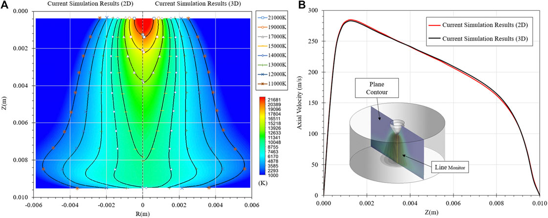
FIGURE 4. (A) Comparison of 2D and 3D simulated isotherms. (B) Comparison of 2D and 3D velocity distribution at the domain centerline.

Validation of Steel Melting

With the validated electric arc modeling, the subsequent melting validation can be conducted. The published experimental and simulation data of the keyhole plasma arc welding process (Jian and Wu, 2015) was employed to validate the accuracy of the local arc-steel heat transfer and force interaction prediction during the steel workpiece melting so that those mechanisms can be further applied on the arc melting simulation of the entire steel ingot. The simulation domain and operating conditions were all modified accordingly based on the reported experimental setup, while the heat transfer and force interaction mechanism in the model were kept the same.

During the melting process, the heat transfer continuously happens at the arc-solid interface, so that the solid workpiece can be efficiently melted beneath the electric arc. Meanwhile, the force interaction between the arc and the liquid steel results in the liquid steel to be pushed away immediately by the high-velocity and high-pressure plasma jet, thus the keyhole solid surface is exposed again. The exposed solid surface can further absorb the heat from the electric arc triggering the melting again. This phenomenon occurs repeatedly throughout the entire process leading to a keyhole created inside the workpiece until it penetrates the entire workpiece. Locally, the steel ingot melting using the electric arc has a similar mechanism. Figure 5A compares the simulated steel workpiece melting with both experimental measurement and simulation data reported by Jian and Wu (2015). The dashed line represents the measurement position of the keyhole solid surface profile, and the solid line is the corresponding simulation results obtained by the group, and the temperature contour of the steel workpiece is the result predicted by the present model. From the comparison with the reported data, the present model gives a good prediction of the keyhole solid surface profile, which matches the measurement data and simulation results given by Jian and Wu (2015). The overall error is less than 10%, which further proves the accurate prediction of the heat transfer and force interaction in the model.

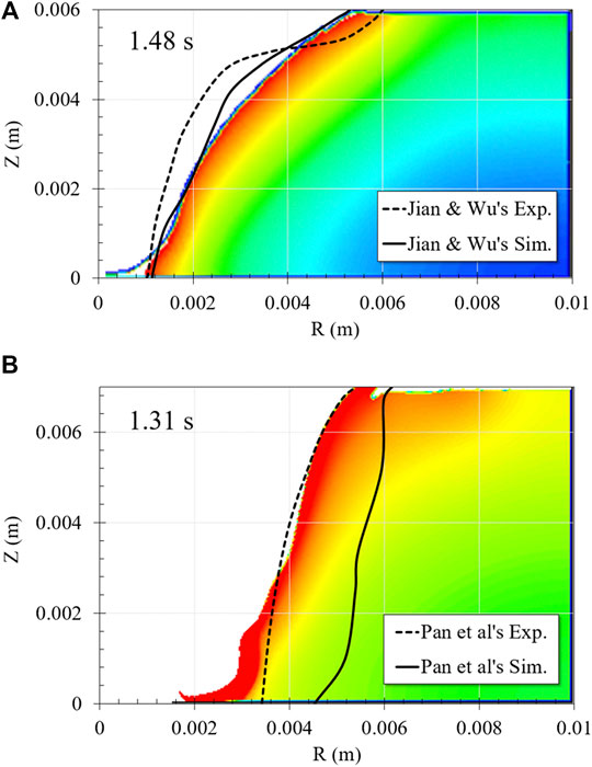
FIGURE 5. Validation of workpiece melting behavior. (A) Use steel as the workpiece. (B) Use aluminum as the workpiece.

Moreover, by modifying the corresponding material properties, the model also has the ability to predict the melting process of other types of metal using electric arc since the overall heat transfer and force interaction mechanism stays the same between the arc and the metal. Figure 5B shows another validation simulation using aluminum as the workpiece based on the experiment reported in Pan et al. (2016). The validation was still conducted by comparing the keyhole solid surface profile in the workpiece to prove the melting prediction to be correct. From the figure, the current simulation results and the reported experimental data given in the figure can well match with each other.

Results and Discussions

Arc Characteristics With Dynamic Electrode Movement

The investigation of the electric arc with varying arc length due to the electrode movement is of great significance for the industrial applications. Maintaining the arc length within a certain range by moving the electrode will help to stabilize the arc, thereby obtaining better arc performance and achieving higher arc melting efficiency. Generally, the sensor calculates the current arc length by detecting the variance of the impedance in the solid material and returns the signal to the controller for consequent action if the arc length changed. For example, if the solid surface collapses due to melting, the arc length will be elongated accordingly and the impedance value will change as well. In this case, the controller will move the electrode downward to shorten the arc length and ensure the arc length return to the preset value to meet the requirement of the production. This process is a continuous regulation process, meaning the arc length is changing dynamically. Thus, it is necessary to have a better understanding of the detailed arc characteristic during this period for better controlling. The present study aims to conduct a quantitative analysis of the effect of dynamic variation of arc length on the arc itself and the melting of the anode surface to provide practical guidance for the operation.

For the simplification purpose, the simulation domain adopted in this section includes the electric arc plasma and the top surface of the solid steel ingot (the anode surface). In order to observe the characteristics of the arc, it is only after the electric arc plasma is generated and stabilized that the electrode begins to move up and down along its axis at a constant velocity. The electrode descends continuously at 0.001 m/s between 0 and 7 s, then changes the direction of movement and lifts up with the same velocity until the end of the simulation. Figure 6 shows the dynamic effect of varying arc length due to electrode movement on the arc characteristics. From Figures 6A,B, as the electrode tip gets closer to the anode surface, the reducing arc length makes the entire arc column be greatly compressed. As a result, the arc loses its original bell shape and the high-temperature area beneath the electrode tip expands. Such conclusions can be observed from the 11,000 K isotherm and the 21,000 K isotherm in the temperature contours. Under the premise of the same arc operating conditions, the energy released due to the ionization of the gas between the electrode tip and the anode surface needs to diffuse outward in the radial direction based on the conservation of energy if the vertical space is reduced, thus the surrounding gas is rapidly heated up and the high temperature region becomes an M-shaped distribution. Figure 7A shows the near-wall gas temperature at the electrode surface during the dynamic descent of the electrode. It can be seen that when the tip-anode vertical distance reduces from 0.01 to 0.003 m, the average temperature increases along the line monitor to reach up to 10,000 K, which may result in great consumption of electrode itself in the practical production. As the electrode turns to move upwards from 7 to 15 s, the arc gradually returns to the bell shape. At the last moment of the simulation (14–15 s), the electrode is lifted up over the original arc length leading the entire arc to be stretched. In reality, such an operation increases the resistance of the arc and cools down the arc, which can be reflected from the shrinking of the 11,000 K isotherm and the 21,000 K isotherm in Figure 6C.

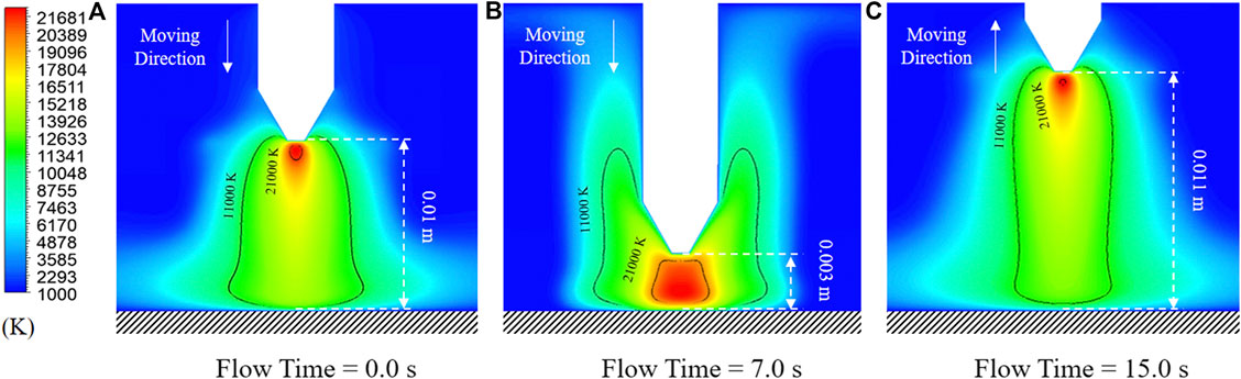
FIGURE 6. Dynamic effect of varying arc length due to electrode movement on the arc characteristics. (A) Flow time = 0.0 s, (B) flow time = 7.0 s, (C) flow time = 15 0 s.

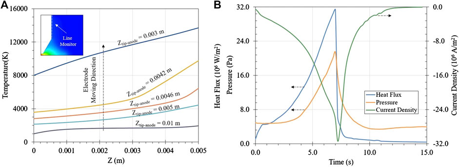
FIGURE 7. (A) Near-wall gas temperature distribution at the electrode surface during the electrode descent. (B) Distribution of the heat flux, pressure and current density at the anode surface during the electrode descent.

Furthermore, the dynamic effect of the arc on the anode surface under varying arc length is further studied. The arc performance is evaluated by analyzing the area-averaged heat flux, pressure, and current density on the anode surface. The changes in these variables over time are shown in Figure 7B. From the figure, the electrode descents to the lowest point in about 7 s. During this time, the area-averaged heat flux, pressure, and current density on the anode surface all show an exponential increase or decrease, and values of those variables reach the peak at around 7 s. The extremely high heat flux and current density significantly enhance the heat conduction between the arc and the anode surface and the generation of a large amount of electronic heat on the anode surface, causing the solid material to have the intensive melting. Meanwhile, the arc also applies a high pressure on the anode surface resulting in the liquid steel being blown away, thereby exposing a new molten solid surface to participate in a new round of melting. Although the short arc length will greatly increase the melting efficiency of the arc based on the previous discussion, the ambient gas surrounding the electrode is more easily heated to the high temperature due to the compression of the arc column. Thus, the electrode consumption rate also increases at the same time. For a long arc, the arc resistance value and the active power consumption are greater, which in turn leads to the reduction of the arc melting efficiency and the poor stability of the arc. Therefore, maintaining a relatively reasonable and stable arc length will balance the electrode consumption rate and melting efficiency to achieve the highest economic benefit.

Steel Ingot Melting With Stationary Electrode

This section first analyzes the melting of a steel ingot using the electric arc under the condition of a fixed electrode position. An initial arc length of 0.01 m is used for the arc ignition. The simulation results of the entire steel ingot melting are shown in Figure 8. At the beginning of the melting stage, the electric arc contacts the ingot top surface in the form of a bell shape and transfers a large amount of heat to it. The heat is Gaussian-distributed from the surface center outwards, thus the entire steel ingot follows the melting sequence from the center to the outside and from the top to the bottom. The red area in the contours represents molten liquid steel. From the first three contours, the high-velocity and high-pressure plasma jet hits the liquid steel that just melted and accumulated in the surface depression, causing it to splash or flow to the edge of the ingot and further drip from its side surface. Since the side surface of the steel ingot is not directly heated by the arc, it still maintains a relatively cold condition. The high-temperature liquid steel dripping along the surface or gathering at the bottom of the crucible transfers its heat to the cold side surface and cools down and solidifies again. Furthermore, as the steel ingot melts, the arc melting efficiency gradually decreases with the arc length increasing. The above two main factors directly cause the solid volume of the steel ingot to decline in a fluctuating manner during the melting process. On the other hand, as the liquid steel is pushed away by the plasma jet, the solid ingot top surface is exposed allowing it to be further melted. The rest of the surface that is still covered by the high-temperature liquid steel melts due to the heat conduction between the solid and the liquid. The above process will be repeated at the beginning and middle melting stages until the remaining solid part is fully immersed in the liquid steel. The last two contours show that the remaining steel ingot is having the in-bath melting. During this period, the main method for the in-bath melting is through the forced convection, that is, the high-temperature liquid steel in the bath is stirred by the strong impact of the electric arc and keeps transferring heat to the immersed solid. The electric arc only heats the liquid steel on the surface of the liquid steel bath.

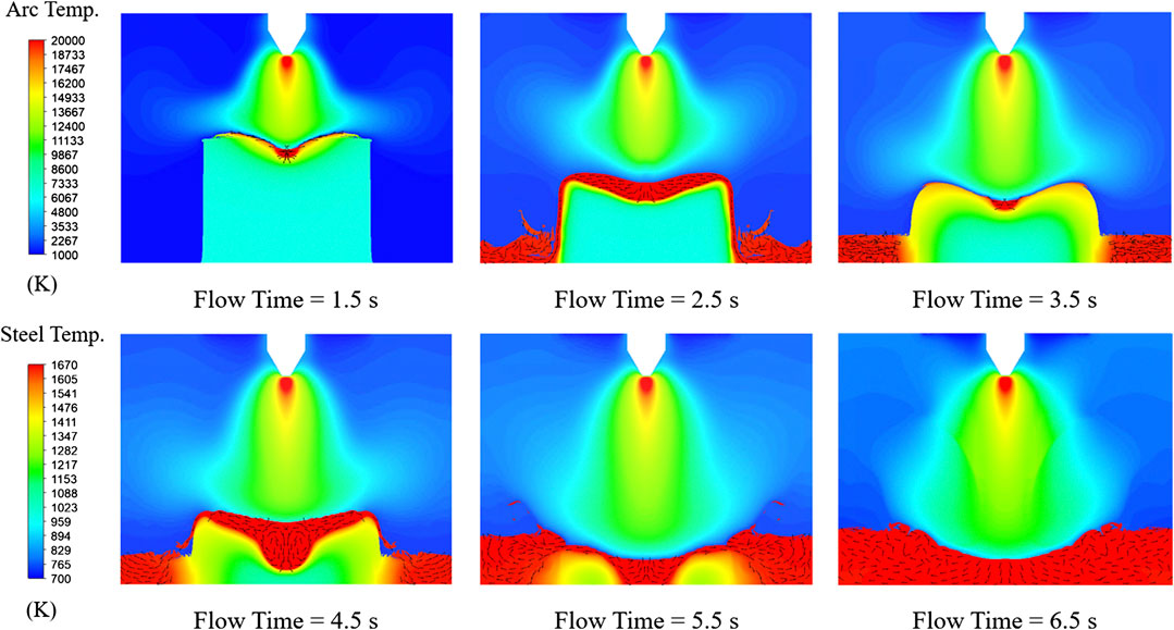
FIGURE 8. Steel ingot melting using electric arc with stationary electrode.

Based on the above discussion, the effect of the initial arc length on the steel ingot melting rate can be further explored. The positions of the fixed electrode are adjusted downward by 0.0025 and 0.005 m, respectively, so that the initial arc lengths can be set to 0.0075 and 0.005 m, respectively. The melting rate is analyzed by comparing the remaining volume of the solid steel ingot, whose results are shown in Figure 9. All three melting curves show a fluctuating decline due to the repeated melting and solidification of steel. The initial arc lengths of 0.01, 0.0075, and 0.005 m correspond to the melting times of 4.4, 5.6, and 6.4 s, respectively. Two identical descending heights of the electrode position reduce the melting times by 12.5 and 21.4%, respectively. Therefore, the initial arc length has a great impact on the steel ingot melting rate. The three temperature contours given at 2 s illustrate that the smaller initial arc length can provide higher instantaneous heat flux and current density, and effectively avoid the accumulation of liquid steel in the surface depression (red area), thus more surface can be directly contacted with the arc to achieve the layer-by-layer melting. Such melting behavior greatly accelerates the overall melting efficiency of the steel ingot, which is consistent with the conclusions discussed before. Therefore, in an actual production, it is recommended to shorten the initial arc length to effectively reduce the arc dissipation and to enhance the arc performance acting on the solid surface, thereby improving the melting efficiency of the steel ingot.

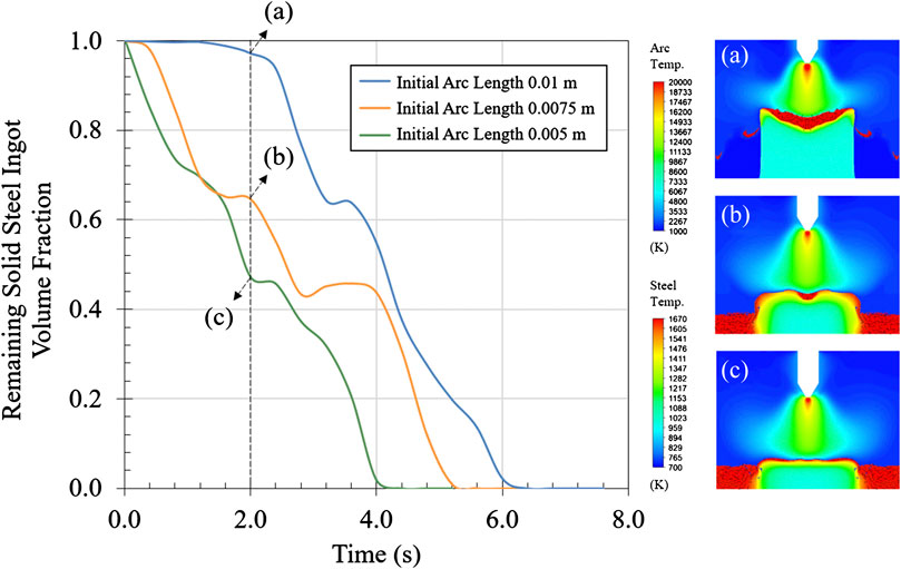
FIGURE 9. Effect of initial arc length on steel ingot melting efficiency with stationary electrode.

Steel Ingot Melting With Dynamic Electrode Movement

This section further considers the steel ingot melting using the electric arc under the dynamic moving electrode. In the cases of using the fixed electrode position, the arc length increases as the height of the steel ingot decreases. According to the previous discussion, longer arc length largely elevates the arc resistance and is not conducive to the stability of the arc, which may easily cause the arc extinction and have a certain impact on the stability of the entire electronic system.

Generally, moving the electrode downward based on the melting rate to ensure a relatively stable arc length is one of the widely-accepted solutions in the actual operation and the most common example is the electrode bore-in during the melting stage in EAF. So far, there is no relevant literature known to the authors that has reported the numerical modeling of melting the steel ingot using the electric arc under the dynamic moving electrode. Thus, it is necessary to conduct further research on this. In the present study, the dynamic mesh is employed to achieve the electrode movement in the model. The electrode descend is assumed to be at a constant velocity of 0.0015 m/s downward in the simulation. The results are shown in Figure 10A. The distance between the electrode tip and the ingot top surface is maintained near the given value of the initial arc length during the entire melting stage. The relatively stable arc length enables the electric arc to sustain good thermodynamic characteristics, so that the arc can keep its original bell shape and melt the surface of the steel ingot with higher heat flux. Under the premise that the initial arc length is 0.01 m, as shown in Figure 10B, the case with the dynamic electrode movement reduces the melting time from 6.4 to 4.8 s, which has a total reduction of 25%.

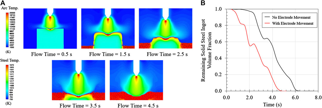
FIGURE 10. (A) Steel ingot melting using electric arc with dynamic moving electrode. (B) Comparison of steel ingot melting efficiency with and without dynamic moving electrode.

Figures 11A,B show the axial temperature and velocity distribution at 0.0005 m above the ingot top surface with and without considering the dynamic movement of the electrode. Since the steel ingot itself continuously melts, the position of the ingot top surface also continuously declines. Thus, 0.0005 m mentioned in the present section is the relative distance from the ingot top surface at the current moment. Both figures show instantaneous temperature and velocity distributions at 0.5, 1.5, and 2.5 s for comparison. From the charts, the case considering the dynamic electrode movement is able to maintain a relatively stable arc length, and the temperature and velocity distribution at the three plotted moments are concentrated and have a similar distribution and numerical range. On the contrary, for the case where the dynamic electrode movement is not considered, the distribution of instantaneous temperature and velocity reaching the ingot top surface is very different from each other. A large reduction can be found for both curves as the arc length continues to increase. According to the data given in Figure 11B, the average peak temperature decreases up to 2000 K per second and the average peak velocity decreases up to 40 m/s per second meaning the original arc performance cannot be maintained in the sequent arc melting, which results in a significant negative impact on the melting efficiency.

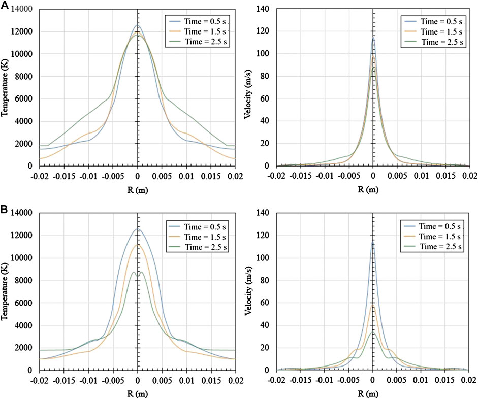
FIGURE 11. (A) Axial temperature and velocity distribution at 0.0005 m above the ingot top surface with the dynamic moving electrode. (B) Axial temperature and velocity distribution at 0.0005 m above the ingot top surface without the dynamic moving electrode.

Application to Electric Arc Furnace Scrap Melting

The numerical model used in the present research can provide a basis for the subsequent simulation of EAF scrap melting. In the steelmaking process of EAF, different types and shapes of scrap are charged into the furnace to form a scrap stack. The electrode is inserted through the electrode holes to strike an arc in-between the electrode tip and the scrap surface to generate a large amount of heat for the scrap melting. Locally, the EAF scrap melting mechanism is similar to the steel ingot melting mechanism considered in the present study. The most obvious difference is that the scrap stack is a porous structure with certain voids inside, which allows the liquid steel dripping through it, while the steel ingot is a solid structure and the liquid steel can only flow on the solid surface. In fact, the model adopted in this research is based on the fixed grid method and volume-of-fluid method to simulate the melting and solidification of solid materials. The specific method to eliminate the movement of the solid phase is by adding the corresponding momentum sink to the momentum equation. However, since the gas-liquid-solid three phases share a single momentum equation, eliminating the movement of the solid phase will cause the flow of any other phase in the grid to be eliminated as well. Therefore, the solid steel ingot region cannot be directly processed as a porous structure by modifying the volume fraction in the corresponding grid. This section presents a potentially feasible method to build a steel ingot stack with voids to achieve a porous structure similar to the EAF scrap steel stack.

The present study adopts the discrete element method to simulate the process of charging each steel ingot in the domain and the data of the final steel ingot distribution is imported into the CFD solver as the initial steel ingot stack, as shown in the first contour in Figure 12. Based on this method, a steel ingot stack composed of a pure solid region and a pure gas region can be obtained and the porosity of the steel ingot stack can be calculated according to the pure solid region volume and the pure gas region volume. The follow-up works can consider more steel ingot shapes in line with the actual situation in addition to the cube used in the current study. It should be noted that the domain considered in the current simulation is still a laboratory-scale crucible rather than an industrial-scale EAF, and electrode movement is also included. The sequent melting simulation of the steel ingot stack is similar to the results shown in previous sections. As the electrode dynamically moves down, the steel ingot stack will gradually melt from inside to outside and from top to bottom. The only difference is that the liquid steel flows through the voids to the bottom and eventually gathers at the bottom to form a liquid steel bath, as shown in the last three contours in Figure 12, which is similar to the scrap melting behavior in industrial EAF.

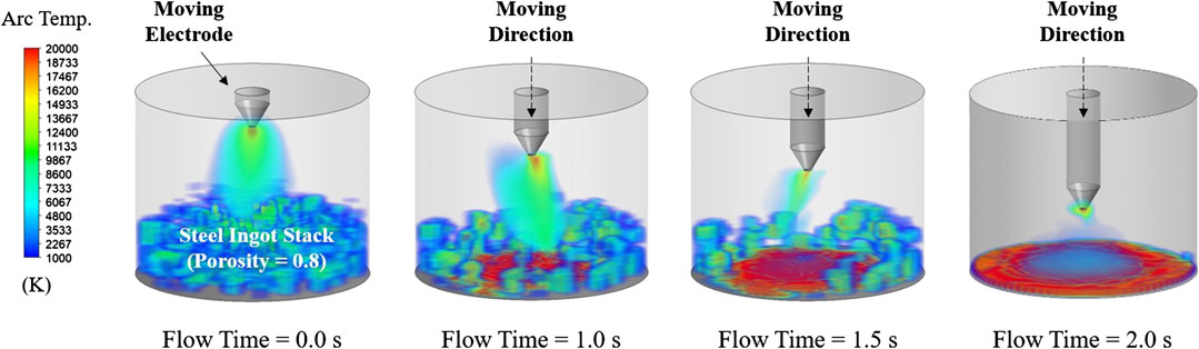
FIGURE 12. Steel ingot stack melting using electric arc with dynamic moving electrode.

Conclusion

The present study established a numerical model to dynamically simulate the entire steel ingot melting process using the electric arc, which includes the continuous phase changing of solid steel, the surface deformation of steel ingot, and the close interaction between phases. The stationary DC electric arc modeling and the arc-solid steel interface heat transfer and force interaction modeling were validated respectively against the experimental data, which proved the model accuracy. The relevant researches were conducted based on the validated model and the following conclusions were made:

1. The DC electric arc behavioral characteristics with varying arc length generated by the electrode movement was analyzed, which reveals that maintaining a reasonable and stable arc length will balance the electrode consumption rate and melting efficiency to achieve the highest economic benefit.

2. The effect of the initial arc length on the melting efficiency was studied, which demonstrates that the smaller initial arc length can provide higher instantaneous heat flux and current density and reduce the arc dissipation, meanwhile effectively avoid the accumulation of liquid steel in the surface depression thus more surface can be directly contacted with the arc to achieve the layer-by-layer melting, which greatly improves the overall melting efficiency.

3. The entire steel ingot melting process using the electric arc under the dynamic moving electrode was simulated, which illustrates that the case considering the dynamic electrode movement can maintain the original arc performance near the ingot top surface in the sequent melting of the steel ingot, which results in a positive impact on the melting efficiency.

4. A potential method was proposed to apply the current model in simulating the EAF scrap melting. The preliminary simulation results of the scrap melting in the lab-scale furnace using this potential method were given.

Data Availability Statement

All datasets generated for this study are included in the article.

Author Contributions

YC: Conceptualization, methodology, model development, model validation and manuscript draft. YC and QL: parametric studies and data post processing. AKS and YC: review and editing. CQZ: project supervision and funding acquisition.

Funding

This research was funded by Steel Manufacturing Simulation and Visualization Consortium (SMSVC).

Conflict of Interest

The authors declare that this study received funding from Steel Manufacturing Simulation and Visualization Consortium (SMSVC). The funder had the following involvement in the study: Monthly progress reviews from Project Technical Committee group, technical consultancy, provision of industrial data.

Acknowledgments

The authors would like to thank the Steel Manufacturing Simulation and Visualization Consortium (SMSVC) members for funding this project. The Center for Innovation through Visualization and Simulation (CIVS) at Purdue University Northwest is also gratefully acknowledged for providing all the resources required for this work. The authors also appreciate the great help from Eugene Pretorius (NUCOR), Yury Krotov (Steel Dynamics, Inc.), Jianghua Li (AK Steel), and Nicholas J. Walla (CIVS).

References

Apelian, D., Paliwal, M., Smith, R. W., and Schilling, W. F. (1983). Melting and solidification in plasma spray deposition - phenomenological review. Int. Mater. Rev. 28 (1), 271–294. doi:10.1179/imtr.1983.28.1.271
Backer, G., and Szekely, J. (1987). The interaction of a DC transferred arc with a melting metal: experimental measurements and mathematical description. Metall. Trans. B 18 (1), 93–104. doi:10.1007/bf02658435
Boulos, M. I., Fauchais, P., and Pfender, E. (2013). Thermal plasmas: fundamentals and applications. New York, NY: Springer Science and Business Media.
Brackbill, J. U., Kothe, D. B., and Zemach, C. (1992). A continuum method for modeling surface tension. J. Comput. Phys. 100 (2), 335–354. doi:10.1016/0021-9991(92)90240-y
Cressault, Y. (2001). Propriétés des plasmas thermiques dans des mélanges argon-hydrogene-cuivre. PhD thesis. Toulouse (France): Université Paul Sabatier.
Dowden, J., and Kapadia, P. (1994). Plasma arc welding: a mathematical model of the arc. J. Phys. D Appl. Phys. 27 (5), 902. doi:10.1088/0022-3727/27/5/004
Fan, H. G., and Kovacevic, R. (1999). Droplet formation, detachment, and impingement on the molten pool in gas metal arc welding. Metall. Mater. Trans. B 30 (4), 791–801. doi:10.1007/s11663-999-0041-6
Freton, P., Gonzalez, J. J., and Gleizes, A. (2000). Comparison between a two- and a three-dimensional arc plasma configuration. J. Phys. D Appl. Phys. 33 (19), 2442. doi:10.1088/0022-3727/33/19/315
Hsu, K. C., Etemadi, K., and Pfender, E. (1983). Study of the free‐burning high‐intensity argon arc. J. Appl. Phys. 54 (3), 1293–1301. doi:10.1063/1.332195
Hu, J., and Tsai, H.-L. (2007). Heat and mass transfer in gas metal arc welding. Part I: the arc. Int. J. Heat Mass Tran. 50 (5–6), 833–846. doi:10.1016/j.ijheatmasstransfer.2006.08.025
Jian, X., and Wu, C. S. (2015). Numerical analysis of the coupled arc-weld pool-keyhole behaviors in stationary plasma arc welding. Int. J. Heat Mass Tran. 84, 839–847. doi:10.1016/j.ijheatmasstransfer.2015.01.069
Lago, F., Gonzalez, J. J., Freton, P., and Gleizes, A. (2004). A numerical modelling of an electric arc and its interaction with the anode: Part I. The two-dimensional model. J. Phys. D Appl. Phys. 37 (6), 883. doi:10.1088/0022-3727/37/6/013
Li, L., Li, B., Liu, L., and Motoyama, Y. (2017). Numerical modeling of fluid flow, heat transfer and arc-melt interaction in tungsten inert gas welding. High Temp. Mater. Process. 36 (4), 427–439. doi:10.1515/htmp-2016-0120
Lowke, J. J. (1979). Simple theory of free-burning arcs. J. Phys. D 12 (11), 1873. doi:10.1088/0022-3727/12/11/016
Lowke, J. J., and Tanaka, M. (2006). ‘LTE-diffusion approximation’ for arc calculations. J. Phys. D 39 (16), 3634. doi:10.1088/0022-3727/39/16/017
Pan, J., Hu, S., Yang, L., and Chen, S. (2016). Numerical analysis of the heat transfer and material flow during keyhole plasma arc welding using a fully coupled tungsten-plasma-anode model. Acta Mater. 118, 221–229. doi:10.1016/j.actamat.2016.07.046
Sames, W. (2015). Additive manufacturing of Inconel 718 using electron beam melting: processing, post-processing, and mechanical properties. PhD thesis. College Station (TX): Texas A&M University.
Tanaka, M., Ushio, M., and Lowke, JJ. (2004). Numerical study of gas tungsten arc plasma with anode melting. Vacuum 73 (3–4), 381–389. doi:10.1016/j.vacuum.2003.12.058
Tashiro, S., Miyata, M., and Tanaka, M. (2011). Numerical analysis of AC tungsten inert gas welding of aluminum plate in consideration of oxide layer cleaning. Thin Solid Films 519 (20), 7025–7029. doi:10.1016/j.tsf.2011.04.137
Wu, C. S., Hu, Q. X., and Gao, J. Q. (2009). An adaptive heat source model for finite-element analysis of keyhole plasma arc welding. Comput. Mater. Sci. 46 (1), 167–172. doi:10.1016/j.commatsci.2009.02.018
Yin, F., Hu, S., Yu, C., and Li, L. (2007). Computational simulation for the constricted flow of argon plasma arc. Comput. Mater. Sci. 40 (3), 389–394. doi:10.1016/j.commatsci.2007.01.008
Keywords: arc melting, electrode movement, heat transfer, electric arc furnace, computational fluid dynamics
Citation: Chen Y, Luo Q, Silaen AK and Zhou CQ (2020) Multi-Physics Modeling of Steel Ingot Melting by Electric Arc Plasma and its Application to Electric Arc Furnace. Front. Mater. 7:576831. doi: 10.3389/fmats.2020.576831
Received: 27 June 2020; Accepted: 02 September 2020;
Published: 08 October 2020.
Edited by:
Qing Liu, University of Science and Technology Beijing, ChinaReviewed by:
Chao Chen, Taiyuan University of Technology, ChinaXiaojun Xi, University of Science and Technology Beijing, China
Copyright © 2020 Chen, Luo, Silaen and Zhou. This is an open-access article distributed under the terms of the Creative Commons Attribution License (CC BY). The use, distribution or reproduction in other forums is permitted, provided the original author(s) and the copyright owner(s) are credited and that the original publication in this journal is cited, in accordance with accepted academic practice. No use, distribution or reproduction is permitted which does not comply with these terms.
*Correspondence: Chenn Q. Zhou, czhou@pnw.edu