A Comparative Study of Several Metaheuristic Algorithms to Optimize Monetary Incentive in Ridesharing Systems

Abstract

The strong demand on human mobility leads to excessive numbers of cars and raises the problems of serious traffic congestion, large amounts of greenhouse gas emissions, air pollution and insufficient parking space in cities. Although ridesharing is a potential transport mode to solve the above problems through car-sharing, it is still not widely adopted. Most studies consider non-monetary incentive performance indices such as travel distance and successful matches in ridesharing systems. These performance indices fail to provide a strong incentive for ridesharing. The goal of this paper is to address this issue by proposing a monetary incentive performance indicator to improve the incentives for ridesharing. The objectives are to improve the incentive for ridesharing through a monetary incentive optimization problem formulation, development of a solution methodology and comparison of different solution algorithms. A non-linear integer programming optimization problem is formulated to optimize monetary incentive in ridesharing systems. Several discrete metaheuristic algorithms are developed to cope with computational complexity for solving the above problem. These include several discrete variants of particle swarm optimization algorithms, differential evolution algorithms and the firefly algorithm. The effectiveness of applying the above algorithms to solve the monetary incentive optimization problem is compared based on experimental results.

1. Introduction

The strong demand on human mobility leads to high use of private cars and raises the problems of serious traffic congestion, large amounts of greenhouse gas emissions, air pollution and insufficient parking space in cities. Ridesharing is a transportation model that can be applied to solve the above problems in cities by sharing cars or vehicles. In the past decade, the subject of ridesharing has attracted the attention of researchers around the world. Survey papers of the studies on ridesharing/carpooling problems can be found in References [1,2]. The results of the exploratory study by Genikomsakis et al. [3] indicate that people maintain a positive attitude towards the ridesharing and carpooling transportation modes. In the literature, several systems have been developed to verify ridesharing/carpooling systems. For example, a carpooling system for universities called PoliUniPool was presented in Reference [4]. In terms of the characteristics and modes of operation, carpooling/ridesharing systems can be classified into daily carpooling problem [5], long-term carpooling problem [6] and dynamic ridesharing problem [7].

To effectively support operations of ridesharing systems, several issues need to be addressed. An important issue is to extract rides that are amenable for ridesharing based on mobility traces. In Reference [8], Bicocchi and Mamei presented a methodology to analyze mobility data for ridesharing. In Reference [9], Toader et al. proposed an indicator for collaborative mobility between individuals based on the use of smartphone data. In Reference [10], a carpooling prototype system was developed to match passengers with drivers based on their trajectories. A carpooling problem was formulated in Reference [11] and a heuristic algorithm was proposed to assign passengers to drivers’ cars based on their trajectories.

1.1. Motivation

Although ridesharing is a potential transportation mode to reduce the excessive number of cars through car-sharing, it is still not widely adopted. Motivated by this fact, there are several papers addressing factors that contribute to carpooling/ridesharing [12,13,14]. All the above studies point out that savings of cost and time are the main incentives for ridesharing. There is an old Chinese idiom that goes, “Human beings die in pursuit of wealth, and birds die in pursuit of food.” When it comes to doing business, it is the profits that count. In the context of ridesharing, providing profits or a monetary incentive for ridesharing participants is one effective way to improve acceptance of the ridesharing model. However, most studies consider non-monetary incentive performance indices such as travel distance and successful matches in ridesharing systems. These performance indices fail to provide a strong incentive for ridesharing. There are only a few works focusing on maximization of cost savings to provide incentives in ridesharing systems.

Santos and Xavier dealt with both dynamic ridesharing and taxi-sharing problems [15]. In their work, passengers and car owners specify their origins, destinations and relevant timing information. Passengers announce the maximum willing to pay price for their rides. Taxi drivers declare the locations and relevant timing information for the provided service. The problem is to match requests to vehicles in such a way that capacity constraints of vehicles and the maximum willing to pay price of each passenger are satisfied. In Reference [16], Watel and Faye studied a Dial-a-Ride problem with money as an incentive (DARP-M). They studied the taxi-sharing problem to reduce the cost of passengers. Watel and Faye defined three variants of the DARP-M problems: max-DARP-M, max-1-DARP-M and 1-DARP-M, to analyze their complexity. The objective of max-DARP-M is to drive the maximum number of passengers under the assumption of unlimited number of taxis available. The max-1-DARP-M problem is used to find the maximum number of passengers that can be transported by a taxi. The 1-DARP-M problem is used to determine whether it is possible to drive at least one passenger under the constraints stated. However, the max-DARP-M, max-1-DARP-M and 1-DARP-M problems are oversimplified and fail to reflect real application scenarios even though they can be used to analyze the complexity of the problems. In addition, the overall monetary incentive in ridesharing systems is not considered in Reference [16]. In Reference [17], Hsieh considered a monetary incentive in ridesharing systems and proposed a metaheuristic solution algorithm for it. However, effectiveness of applying different metaheuristic algorithms to solve the problem formulated in Reference [17] needs further study.

Most ridesharing problems can be formulated as optimization problems. Several meta-heuristic approaches to deal with the complexity issue in optimization problems have been developed in the past [18] and applied in different problem domains [19]. Genetic algorithm (GA) and swarm intelligence [20,21,22] are two well-known population-based meta-heuristic approaches. GA maintains a population of candidate solutions and attempts to improve the candidate solutions based on biologically inspired operators such as mutation, crossover and selection to guide the search. Swarm intelligence is also a population-based meta-heuristic approach relying on a collective behavior of decentralized, self-organized agents in the population, called a swarm. In the literature, well-known meta-heuristic approaches proposed based on swarm intelligence include particle swarm optimization (PSO) [23], firefly algorithm [24] and monarch butterfly optimization [25]. In the literature, swarm intelligence-based approaches, such as PSO, have several advantages over GA [26,27]. In addition to GA and swarm intelligence, evolutionary computation has been proposed and widely applied in solving different problems [28]. Differential evolution (DE) [29] is a population-based metaheuristic approach in evolutionary computation. DE attempts to improve the solutions in the population by creating new trial solutions through combining existing ones. Better trial solutions will replace the existing solutions in the population.

Although many metaheuristic algorithms such as the PSO algorithm [23], firefly algorithm [24] and differentiation evolution (DE) algorithm [29] have been proposed and applied to solve a variety of optimization problems with continuous solution space for decades, effectiveness of these metaheuristic algorithms in solving optimization problems with discrete solution space is less addressed. As the earlier versions of the PSO algorithm, firefly algorithm and DE algorithm were proposed to find solutions for optimization problems with continuous solution space, these algorithms must be modified properly to be applied to optimization problems with discrete solution space. Kennedy and Eberhart proposed a reworking of the PSO algorithm for problems with discrete binary variables in Reference [30]. During the past years, several variants of PSO algorithms and DE algorithms have been proposed in References [31] and [32] for the ridesharing problem with a linear objective function. However, effectiveness of applying these variants of algorithms to solve the nonlinear monetary incentive optimization problem requires further study. In particular, the results in Reference [31] indicate that the cooperative coevolving particle swarm optimization algorithm outperforms other metaheuristic algorithms for the ridesharing problem with a linear objective function by combining the strategies of decomposition with random grouping with cooperative coevolution [33,34,35]. Whether the cooperative, coevolving particle swarm optimization algorithm still outperforms other variants for the problem defined in Reference [17] is an interesting question.

1.2. Research Question, Goals and Objectives

Based on the discussion on deficiencies of existing studies above, the research questions addressed in this study are as follows: How to deal with monetary incentive issue in ridesharing systems and formulate the decision problem? How to develop metaheuristic algorithms for this problem? How about effectiveness of different metaheuristic algorithms for solving this decision problem? The goals of this paper are to answer the above questions through the development of a solution methodology. The objectives of this paper are to (1) address the monetary incentive issue in ridesharing systems by proposing a monetary incentive performance indicator to improve the incentives for ridesharing, (2) formulate the monetary incentive optimization problem, (3) develop solution metaheuristic algorithms based on modification of several variants of PSO algorithms, DE algorithms and firefly algorithm for the nonlinear monetary incentive optimization problem and (4) study the effectiveness of these metaheuristic algorithms based on the results of experiments. For the optimization of monetary incentive in ridesharing systems, a non-linear integer programming optimization problem is formulated. As finding a solution for the non-linear integer programming optimization problem is computationally challenging, metaheuristic approaches are adopted to solve the problem. The contributions of this paper include: (1) proposing a problem formulation and associated solution algorithms to find and benefit the drivers and passengers with the highest monetary incentive for ridesharing and (2) comparing the effectiveness of several metaheuristic algorithms to provide a guideline for selecting an algorithm to solve the formulated problem.

The monetary incentive optimization problem is a non-linear integer programming problem with a large number of constraints. The computational complexity arises from constraints in the problem formulation. An effective method to deal with constraints must be employed to develop a solution algorithm. In the literature, several ways to deal with constraints in constrained optimization problems have been proposed. The concept behind these constraint-handling methods can be classified into three categories: preserving feasibility of solutions, penalizing infeasible solutions and biasing feasible over infeasible solutions. Among the well-known methods to handle constraints, the penalty function method [36,37] and the biasing feasible over infeasible solutions method [38] are the most popular ones. The biasing feasible over infeasible solutions method does not rely on setting of penalty coefficients or parameters to handle constraints. Therefore, we adopt a method based on biasing feasible over infeasible solutions [36] to develop metaheuristic algorithms. As the solutions evolve in the continuous space, transformation of solutions to discrete space is required for each metaheuristic algorithm developed in this study.

To assess effectiveness of the proposed metaheuristic algorithms, we conduct experiments for several test cases. The numerical results indicate that the discrete variant of the cooperative, coevolving particle swarm optimization algorithm is significantly more effective than other metaheuristic algorithms in solving a constrained optimization problem with nonlinear objective function and binary decision variables. The results confirm the effectiveness of the proposed algorithm.

This paper is different from the brief paper in Reference [17] in that it is extended with a number of metaheuristic algorithms and a comparative study of these metaheuristic algorithms through experiments. As this paper focuses on optimization of monetary incentive in ridesharing systems, it is also different from the work in Reference [31] in two aspects. The objective function is not separable with respect to the decision variables and is a nonlinear function. This makes the optimization problem hard to solve. The problem formulated in this paper is a nonlinear integer programming problem with discrete decision variables, which is different from the one studied in References [10,31].

The remainder of this paper is organized as follows. In Section 2, we describe and formulate the monetary incentive optimization problem. The fitness function and constraint handling method are described in Section 3. The metaheuristic algorithms will be presented in Section 4. In Section 5, we will present and discuss the results. In Section 6, we conclude this paper.

2. Problem Formulation

In this section, the problem formulation will be introduced. The notations required for problem formulation are summarized in

Table 1. Notations of variables/symbols for problem formulation.

Variable/Symbol	Meaning
$P$	total number of passengers
$p$	the ID of a passenger, where $p\in \{1,2,3,\dots ,P\}$
$D$	total number of drivers
$d$	the ID of a driver, where $d\in \{1,2,3,\dots ,D\}$
$K$	total number of locations of passengers, $K=P$
$k$	the location ID, $k\in \{1,2,\dots ,K\}$
$s_{pk}$	the number of seats requested by passenger $p$ for location $k$, where $k\in \{1,2,3,\dots ,K\}$
$J_d$	the number of bids placed by driver $d\in \{1,2,\dots ,D\}$
$j$	the $jth$ bid submitted by driver $d$, where $j\in \{1,2,\dots ,J_d\}$
$c_{dj}$	the routing cost for transporting the passengers in the $jth$ bid submitted by driver $d$
$o_{dj}$	the original travel cost of driver $d$ (without transporting any passenger)
$q_{djk}$	the number of seats available at location $k$ in the $jth$ bid submitted by driver $d$
$D{B}_{dj}$	$D{B}_{dj}=(q_{dj1},q_{dj2},q_{dj3},\dots ,q_{djK},o_{dj},c_{dj})$, the $jth$ bid submitted by driver $d$
$f_p$	the original price of passenger $p$ (without ridesharing)
$P{B}_p$	$P{B}_p=(s_{p1},s_{p2},s_{p3},\dots ,s_{pK},f_p)$: the bid submitted by passenger $p$. The bid $P{B}_p$ is an offer to pay the price $f_{ph}$ for transporting $s_{pk}$ passengers for each $k\in \{1,2,3,\dots ,K\}$
$x_{dj}$	a binary decision variable: it indicates whether the $jth$ bid placed by driver $d$ is a winning bid ($x_{dj}$ = 1) or not ($x_{dj}$ = 0)
$y_p$	a binary decision variable: it indicates whether the bid placed by passenger $p$ is a winning bid ($y_p$ = 1) or not ($y_p$ = 0)

. A ridesharing system consists of a number of passengers, a number of drivers and the cars owned by drivers. To describe the ridesharing problem, we use $P$ to denote the number of passengers in the system and a passenger is referred to as $p$, where $p\in \{1,2,3,\dots ,P\}$. Similarly, we use $D$ to denote the number of drivers in the system and a driver is referred to as $d$, where $d\in \{1,2,3,\dots ,D\}$. For simplicity, it is assumed that each driver owns one car and we use $d$ to refer to the car of driver $d$ whenever it is clear from the context.

The main function of ridesharing systems is to match the set $D$ of drivers with the set $P$ of passengers according to their requirements. To describe the itinerary of driver $d$, let $L{o}_d$ and $L{e}_d$ be the origin and destination of driver $d$, respectively. $R_d$ = $(L{o}_d,L{e}_d)$ denotes the itinerary of driver $d\in \{1,2,3,\dots ,D\}$. Similarly, to describe the itinerary of passenger $p\in \{1,2,3,\dots ,P\}$, we use $L{o}_p$ and $L{e}_p$ to denote the origin and destination of passenger $p$, respectively. $R_p$ = $(L{o}_p,L{e}_p)$ represents the itinerary of passenger $p$.

To formulate the monetary incentive optimization problem in ridesharing systems, the variables/symbols and their meaning are defined in Table 1.

In the ridesharing system considered in this study, drivers and passengers express their transportation requirements by submitting bids. Before submitting bids, it is assumed that drivers and passengers apply some bid generation software to generate bids. For example, the Bid Generation Procedures in Appendix II of Reference [31] may be applied to generate bids for drivers and passengers. However, the problem formulation to be presented below does not presume the use of Bid Generation Procedures in Appendix II of Reference [31] to generate bids. Drivers and passengers may apply any other bid generation software to generate bids. The bids generated for each driver are based on his/her itinerary, $R_d$. Let $J_d$ denote the number of bids generated and submitted by driver $d$. The $jth$ bid submitted by driver $d$ is represented by $D{B}_{dj}$ = $(q_{dj1},q_{dj2},q_{dj3},\dots ,q_{djK},o_{dj},c_{dj})$. The input data $c_{dj}$ and $o_{dj}$ corresponding to the routing cost and the original travel cost of the $jth$ bid of driver $d$ can be measured in any currency (such as USD, EURO, RMB, NT, etc.) appropriate for a specific application scenario.

Similarly, the bid generated for a passenger $p$ is also based on his/her itinerary, $R_p$. It is assumed that each passenger $p$ submits only one bid. The bid generated and submitted by passenger $p$ is represented by $P{B}_p$ = $(s_{p1},s_{p2},s_{p3},\dots ,s_{pK},f_p)$. The parameter $f_p$ denoting the original price of passenger $p$ without ridesharing can be measured in any currency (such as USD, EURO, RMB, NT, etc.) appropriate for a specific application scenario. A bid $P{B}_p$ is called a winning bid if passenger $p$ is selected by the ridesharing system to share a ride with a driver.

The problem is to match drivers and passengers based on their itineraries to optimize monetary incentive. An objective function defined based on the ratio between the cost savings and the original costs is proposed to achieve this goal. The objective function is defined as follows:

$$F(x,y)=\frac{\left[\left({\displaystyle \sum _{p=1}^P{y}_p\left(f_p^{}\right)}\right)-\left({\displaystyle \sum _{d=1}^D{\displaystyle \sum _{j=1}^{J_d}}{x}_{dj}(c_{dj}-o_{dj})}\right)+\left({\displaystyle \sum _{p=1}^P{y}_p\left(T_{}^P{f}_p\right)}\right)+\left({\displaystyle \sum _{d=1}^D{\displaystyle \sum _{j=1}^{J_d}}{x}_{dj}{T}_{}^D(c_{dj}-o_{dj})}\right)\right]}{\left({\displaystyle \sum _{p=1}^P{y}_p\left(f_p^{}\right)}\right)+\left({\displaystyle \sum _{d=1}^D{\displaystyle \sum _{j=1}^{J_d}}{x}_{dj}{c}_{dj}}\right)}$$

(1)

Based on the above monetary objective function, the objective of the monetary incentive optimization problem is to find the set of passengers and drivers such that the ratio between the cost savings and the original costs is maximized. We formulate the following optimization problem:

$$\underset{x,y}{\max }F(x,y)$$

(2)

$$\begin{array}{l}s.t\\ {\displaystyle \sum _{d=1}^D{\displaystyle \sum _{j=1}^{J_d}{x}_{dj}{q}_{djk}}\ge {\displaystyle \sum _{p=1}^P{y}_p{s}_{pk}}}\forall \mathrm{k}\in \{1,2,\dots ,\mathrm{K}\}\end{array}$$

(3)

$${\displaystyle \sum _{p=1}^P{y}_p{f}_p^{}}+{\displaystyle \sum _{d=1}^D{\displaystyle \sum _{j=1}^{J_d}}{x}_{dj}{o}_{dj}}\ge {\displaystyle \sum _{d=1}^D{\displaystyle \sum _{j=1}^{J_d}}{x}_{dj}{c}_{dj}}$$

(4)

$${\displaystyle \sum _{j=1}^{J_d}}{x}_{dj}\le 1\forall d\in \{1,\dots ,D\},\forall j\in \{1,2,\dots ,J_d\}$$

(5)

$$x_{dj}\in \{0,1\}\forall d,\forall j$$

(6)

$$y_p\in \{0,1\}\forall p$$

(7)

The problem is subject to several constraints: (a) the capacity constraints in Equation (3), (b) the cost savings constraints in Equation (4) and (c) the winning bid constraint for each driver in Equation (5). In addition, the values of decision variables must be binary, as specified in Equation (6) and Equation (7). Note that the objective function $F(x,y)$ for the optimization of monetary incentive is nonlinear. It is more complex than the simple linear function in Reference [31].

3. Fitness Function and Constraint Handling Method

The problem formulated previously is a constrained optimization problem with binary decision variables and rational objective function. The objective function $F(x,y)$ in the above optimization problem is not an additively separable function, which is different from the additively separable objective function used in Reference [31]. In addition, the computational complexity arises from constraints in the problem formulation. An effective method to deal with constraints must be employed to develop a solution algorithm.

In existing literature, several ways to deal with constraints in the constrained optimization problem have been proposed and used in solving constrained optimization problems. The concept behind these constraint-handling methods includes preservation of solutions’ feasibility, penalizing infeasible solutions and discrimination of feasible/infeasible solutions. Among the well-known methods to handle constraints, the penalty function method [36,37] and the discrimination of feasible/infeasible solutions method [38] are widely used methods.

Although the penalty function method is very easy to use, it relies on proper setting of the penalty coefficients. The performance of the penalty function method depends on the penalty coefficients. Improper penalty coefficients often seriously degrade the performance. In addition, there still lacks a good way to set the penalty coefficients properly. The approach of discriminating feasible/infeasible solutions method works without relying on coefficients or parameters to handle constraints. Therefore, we adopt the approach of discriminating feasible/infeasible solutions [38]. The details of applying this approach are described below.

The discriminating feasible/infeasible solutions method characterizes a feasible solution with the corresponding original objective function value. For an infeasible solution, instead of calculating the fitness function value due to infeasible solutions, the method of discriminating a feasible/infeasible solutions method characterizes the fitness function value of infeasible solutions based on the objective function value of the current population’s worst feasible solution. In this way, the performance degradation due to improper setting of penalty coefficients can be avoided.

As the discriminating feasible/infeasible solutions method [38] is adopted to handle constraints, we need to find the objective function value of the current population’s worst feasible solution. To achieve this, we define $S_f$ = $\{(x,y)|(x,y)\}$ as a feasible solution in the current population satisfying constraints (3)~(7). Then, the objective function value of the current population’s worst feasible solution can be calculated by $S_{f\min }=\underset{(x,y)\in S_f}{\min }F(x,y)$.

For the discriminating feasible/infeasible solutions method, we define the fitness function $F_1(x,y)$ as follows:

• $F_1(x,y)=\{\begin{array}{l}F(x,y)if(x,y)satisfiesconstraints(3)~(7)\\ U_1(x,y)otherwise\end{array}$, where
• $U_1(x,y)=S_{f\min }+U_2(x,y)+U_3(x,y)+U_4(x,y)$
• $U_2(x,y)={\displaystyle \sum _{k=1}^K(}\min ({\displaystyle \sum _{d=1}^D{\displaystyle \sum _{j=1}^{J_d}{x}_{dj}{q}_{djk}}-{\displaystyle \sum _{p=1}^P{y}_p{s}_{pk},0.0))}},$
• $U_3(x,y)=\min ({\displaystyle \sum _{p=1}^P{y}_p{f}_p^{}}-{\displaystyle \sum _{d=1}^D{\displaystyle \sum _{j=1}^{J_d}}{x}_{dj}(c_{dj}-o_{dj}),0.0)},$
• $U_4(x,y)={\displaystyle \sum _{d=1}^D{\displaystyle \sum _{j=1}^{J_d}\min }}(1-{\displaystyle \sum _{k=1}^K}{x}_{dj},0.0)$

4. Implementation of Discrete Metaheuristic Algorithms

In this study, several discrete versions of metaheuristic algorithms for solving the monetary incentive optimization problem have been developed. The notations required for describing these metaheuristic algorithms are summarized in

Table 2. Notations of variables/symbols for metaheuristic algorithms.

Variable/Symbol	Meaning
$MAX\_GEN$	the maximum number of generations
$t$	the iteration/generation variable
$NP$	population size.
$N$	the problem dimension, where $N={\displaystyle \sum _{d=1}^D{J}_d}+P$
$z_i$	the position of particle $i$, where $i\in \{1,2,\dots ,NP\}$, and $z_i$ = ($x_i$, $y_i$), $x_i$ is the position vector associated with the decision variable $x$ and yi is the position vector associated with the decision variable $y$
$v_i$	the velocity of particle $i$; $v_{in}$ denotes the $n$ element of the vector $v_i$
$P{z}_i$	the personal best of particle $i$, where $i\in \{1,2,\dots ,NP\}$, and $P{z}_{in}$ is the $nth$ element of the vector $P{z}_i$, $n\in \{1,2,\dots ,N\}$
$Gz$	the global best, and $G{z}_n$ is the $nth$ element of the vector $Gz$, where $n\in \{1,2,\dots ,N\}$
$c_1$	a non-negative real parameter less than 1
$c_2$	a non-negative real parameter less than 1
$r_1$	a random variable with uniform distribution $U(0,1)$
$r_2$	a random variable with uniform distribution $U(0,1)$
$V_{\max }$	the maximum value of velocity
$s(v_{in})$	the probability of the bit $v_{in}$
$p_c$	the learning probability, where $p_c$ is greater than 0 and less than 1
$rp$	a random variable with uniform distribution $U(0,1)$
$NS$	total number of swarms
$S{W}_s$	a swarm, where $s\in \{1,2,\dots ,NS\}$
${\omega }_1$ and ${\omega }_2$	weighting factors for updating velocity; $0\le {\omega }_1\le 1$; ${\omega }_1+{\omega }_2=1$
$\theta$	a scaling factor for updating velocity; $\theta >0$
$DS$	a set of integers
$ds$	an integer $ds$ is selected from $DS$
$\widehat{z}$	t ${\omega }_1$ he context vector obtained by concatenating the global best particles from all $NS$ swarms
$S{W}_s.z_i$	the $ith$ particle in the $sth$ swarm $S{W}_s$
$S{W}_s.z_i^p$	the personal best of the $ith$ particle in swarm $S{W}_s$
$S{W}_s.\widehat{z}$	the global best of the component of the swarm $S{W}_s$
$r_{ij}$	the distance between firefly $i$ and firefly $j$
$\gamma$	the light absorption coefficient
${\beta }_0$	the attractiveness when the distance $r_{ij}$ between firefly $i$ and firefly $j$ is zero
${\beta }_0{e}^{-\gamma r_{ij}^2}$	the attractiveness when the distance $r_{ij}$ between firefly i and firefly j
${\epsilon }_{in}^t$	a random number generated from a uniform distribution in [0, 1]
${\alpha }^t$	a constant parameter in [0, 1]
$T(x)$	$T(x)$ = $\frac{e^{2\left|x\right|}-1}{e^{2\left|x\right|}+1}$ a function to transform a real value into a value in $[0,1]$
$CR$	the crossover rate
$F$	the scale factor
$F_i$	the scale factor for individual i
$t{v}_i$	a mutant vector for individual i

. These metaheuristic algorithms include discrete PSO, discrete comprehensive learning particle swarm optimization (CLPSO) [39], discrete DE, discrete firefly, discrete adaptive learning particle swarm optimization (ALPSO) and discrete cooperative coevolving particle swarm optimization (CCPSO) algorithms. All these algorithms will be compared by conducting experiments in the next section. As all these discrete algorithms are developed based on transformation of continuous solutions to binary solutions, all the algorithms mentioned above will be presented in this paper with the exception of the discrete ALPSO algorithm. Just like other algorithms to be presented in this section, the discrete ALPSO is also developed [40] by adding procedure to transform continuous solution space to binary solution space in the evolution processes. Therefore, the discrete ALPSO algorithm will not be presented in this section to save space. For each algorithm presented in this section, the stopping criteria is based on the maximum number of generations parameter, $MAX\_GEN$.

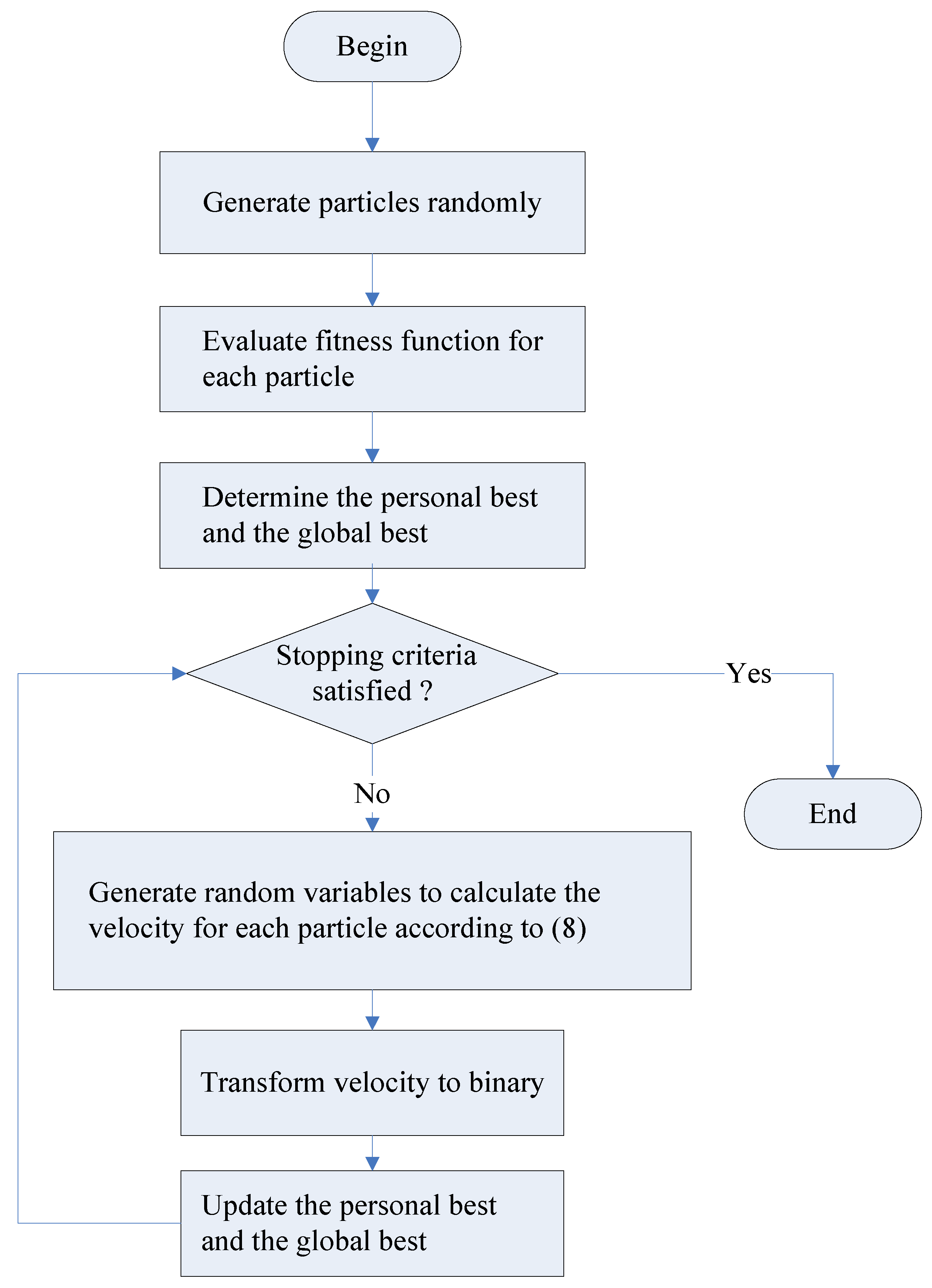
4.1. Discrete PSO Algorithm

The original standard PSO algorithm was proposed in Reference [23] to solve problems with continuous solution space. In the standard PSO algorithm, each particle of the swarm adjusts its trajectory based on its own flying experience as well as the flying experiences from other particles. Let $v_i=(v_{i1},v_{i2},v_{i3},\dots ,v_{iN})$ and $z_i=(z_{i1},z_{i2},z_{i3},\dots ,z_{iN})$ be the velocity and position of particle $i$, respectively. Let $P{z}_i=(P{z}_{i1},P{z}_{i2},P{z}_{i3},\dots ,P{z}_{iN})$ be the best historical position (the personal best) of particle $i$. Let $Gz=(G{z}_1,G{z}_2,G{z}_3,\dots ,G{z}_N)$ be the best historical position (the global best) of the entire swarm. The velocity and position of particle i on dimension $n$ in iteration $t+1$, where $n\in \{1,2,3,\dots ,N\}$, are updated as follows:

$$v_{in}\leftarrow \omega v_{in}+c_1{r}_1(P{z}_{in}-z_{in})+c_2{r}_2(G{z}_n-z_{in})$$

(8)

$$z_{in}\leftarrow z_{in}+v_{in}$$

(9)

where $\omega$ is a parameter called the inertia weight, $c_1$ and $c_2$ are positive constants referred to as cognitive and social parameters respectively, and $r_1$ and $r_2$ are random numbers generated from a uniform distribution in the region of [0, 1].

As the original PSO algorithm was proposed to solve problems with continuous solution space, it cannot be applied to solve the optimization problem with binary decision variables. Therefore, transformation of solutions from continuous space to binary space is required. As the solution space of the optimization problem formulated is binary, we define a procedure $CS(a)$ in

Table 3. The pseudocode for procedure $CS(a)$.

Procedure$CS(a)$

If $a>V_{\max }$ $a\leftarrow V_{\max }$ End If If $a<-V_{\max }$ $a\leftarrow -V_{\max }$ End If $s(a)=\frac{1}{1+{\exp }^{-a}}$ Generate a random variable $rsid$ with uniform distribution $U(0,1)$ $b=\{\begin{array}{l}1rsid<s(a)\\ 0otherwise\end{array}$ Return $b$

to transform continuous solution (CS) space to binary solution space. The procedure $CS(a)$ will be invoked as needed in different variants of PSO algorithms and DE algorithm.

Figure 1 shows the flowchart for the discrete PSO algorithm.

Table 4. The pseudocode for the discrete PSO algorithm.

Discrete PSO Algorithm

$t\leftarrow 0$ Generate particle $z_i$ for each $i\in \{1,2,\dots ,NP\}$ in the population Evaluate the fitness function $F_1(z_i)$ for particle $z_i$, where $i\in \{1,2,\dots ,NP\}$ Determine the personal best $P{z}_i$ for each $i\in \{1,2,\dots ,NP\}$ Determine the global best $Gz$ of swarm While (stopping criteria not satisfied) $t\leftarrow t+1$ For each $i\in \{1,2,\dots ,NP\}$  For each $n\in \{1,2,\dots ,N\}$   Generate a random variable $r_1$ with uniform distribution $U(0,1)$   Generate a random variable $r_2$ with uniform distribution $U(0,1)$   Calculate the velocity of particle $z_i$   $v_{in}\leftarrow v_{in}+c_1{r}_1(P{z}_{in}-z_{in})+c_2{r}_2(G{z}_n-z_{in})$   Transform each element of $v_{in}$ into one or zero   ${\overline{u}}_{in}\leftarrow CS(v_{in})$  End For  Update personal best and global best   If $F_1({\overline{u}}_i)\ge F_1(P{z}_i)$     $P{z}_i$ = $u_i$    End If   If $F_1(P{z}_i)\ge F_1(Gz)$     $Gz$ = $P{z}_i$    End If End While

shows the pseudocode for the discrete PSO algorithm.

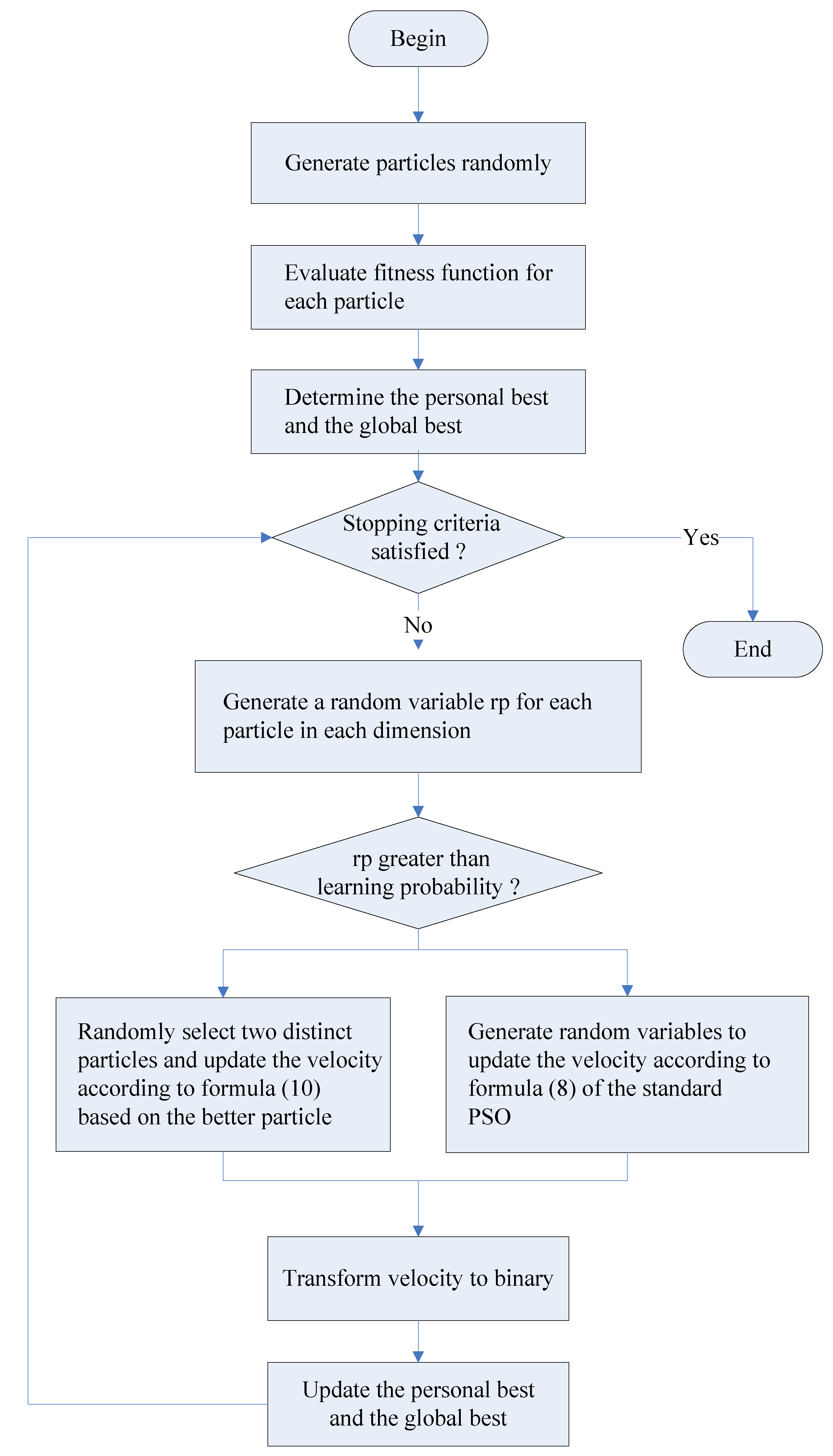
4.2. Discrete CLPSO Algorithm

The CLPSO algorithm [40] is a well-known variant of the PSO algorithm. The CLPSO algorithm works based on the learning probability, $p_c$, where $p_c$ is greater than 0 and less than 1. The CLPSO algorithm generates a random number for each dimension of particle $i$. The corresponding dimension of particle $i$ will learn from its own personal best in case the random number generated is larger than $p_c$. Otherwise, the particle will learn from the personal best of the better of two randomly selected particles, $m_1$ and $m_2$. Let $m$ denote the better particle. The velocity of the particle in dimension $n$ will be updated according to (10) as follows:

$$v_{in}\leftarrow v_{in}+c_1{r}_1(P{z}_{mn}-z_{in})$$

(10)

As the original CLPSO algorithm was proposed to solve problems with continuous solution space, it cannot be applied to solve the optimization problem with binary decision variables. Therefore, transformation of solutions from continuous space to binary space is needed. Figure 2 shows the flowchart for the discrete CLPSO algorithm.

Table 5. The pseudocode for the discrete CLPSO algorithm.

Discrete CLPSO Algorithm

t ← 0 Generate particle $z_i$ for each $i\in \{1,2,\dots ,NP\}$ in the population Evaluate the fitness function $F_1(z_i)$ for each $i\in \{1,2,\dots ,NP\}$ Determine the personal best $P{z}_i$ of each particle Determine the global best $Gz$ of the swarm While (stopping criteria not satisfied) t ← t + 1 For each $i\in \{1,2,\dots ,NP\}$   For each $n\in \{1,2,\dots ,N\}$    Generate a random variable $rp$ with uniform distribution $U(0,1)$    If $rp$ > $p_c$     Generate $r_1$, a random variable with uniform distribution $U(0,1)$     Generate $r_2$, a random variable with uniform distribution $U(0,1)$     Calculate the velocity of particle $i$ as follows     $v_{in}\leftarrow v_{in}+c_1{r}_1(P{z}_{in}-z_{in})+c_2{r}_2(G{z}_n-z_{in})$    else      Randomly select two distinct integers $m_1$ and $m_2$ from $\{1,2,\dots ,NP\}$     If $F_1(z_{m_1})>F_1(z_{m_2})$      Calculate the velocity of particle $i$ as follows      $v_{in}\leftarrow v_{in}+c_1{r}_1(P{z}_{m_{1}n}-z_{in})$     Else      Calculate the velocity of particle i as follows      $v_{in}\leftarrow v_{in}+c_1{r}_1(P{z}_{m_{2}n}-z_{in})$     End If    End If    Transform each element of $v_{in}$ into one or zero    ${\overline{u}}_{in}\leftarrow CS(v_{in})$   End For   Update personal best and global best   If $F_1({\overline{u}}_i)\ge F_1(P{z}_i)$     $P{z}_i$ = $u_i$   End If   If $F_1(P{z}_i)\ge F_1(Gz)$    $Gz$ = $P{z}_i$   End If End While

shows the pseudocode for the discrete CLPSO algorithm.

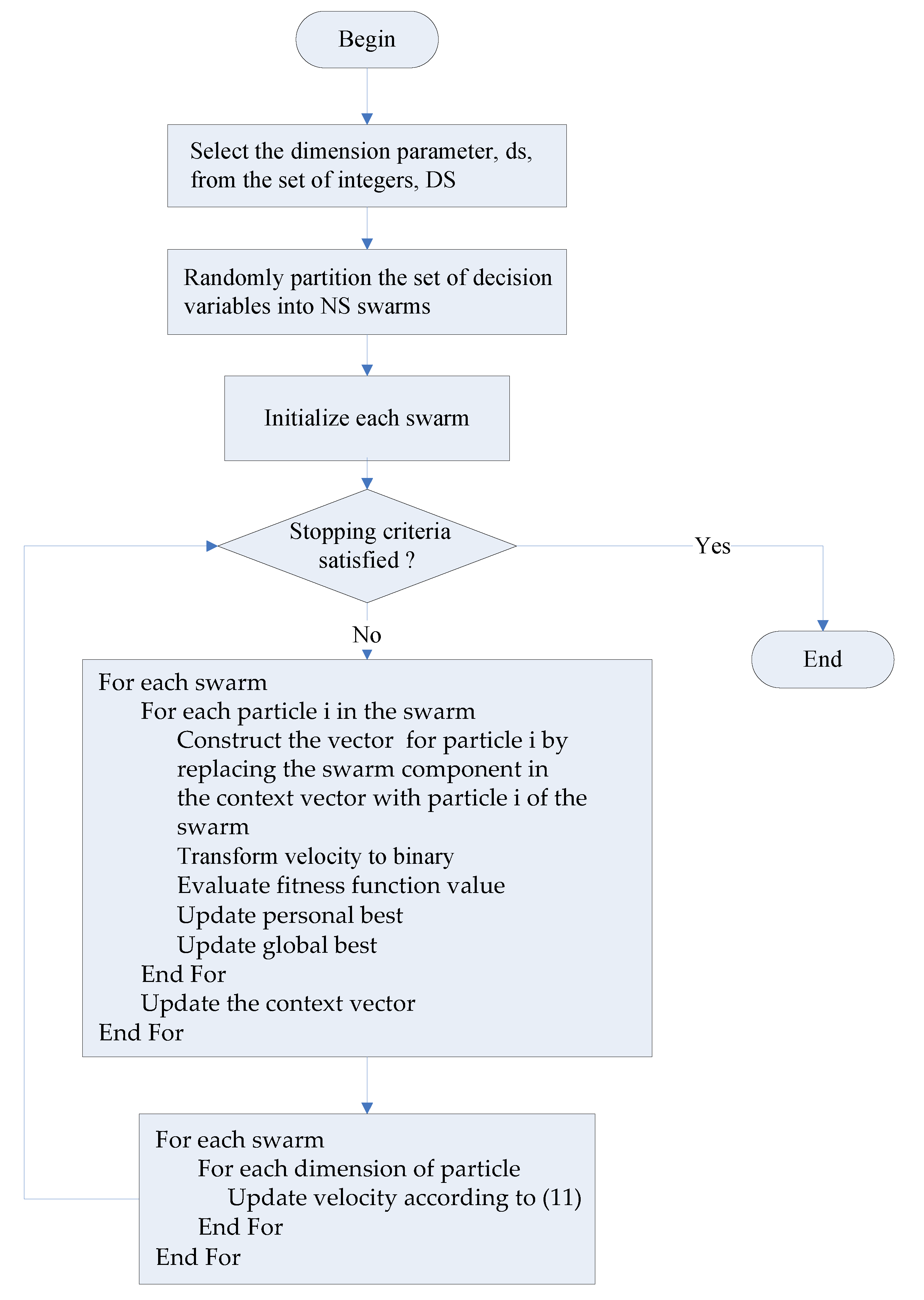
4.3. Discrete CCPSO Algorithm

The discrete CCPSO algorithm adopts a divide-and-conquer strategy to decompose a problem into smaller ones. To decompose the original higher dimensional problem into smaller subproblems, a set of integers, $DS$, is defined first. Then, an integer $ds$ is first selected from $DS$. The discrete CCPSO algorithm decomposes the decision variables into $NS$ swarms based on the selected integer $ds$. To present the discrete CCPSO algorithm, let $z$ be the vector obtained by concatenating decision variables $x$ and $y$ of the problem formulation. To share information in the cooperative coevolution processes, let $\widehat{z}$ be the context vector obtained by concatenating the global best particles from all $NS$ swarms. There are three algorithmic parameters used to update particles in the discrete CCPSO algorithm. These parameters include the weighting factor ${\omega }_1$ and ${\omega }_2$ as well as the scaling factor $\theta$. The $ith$ particle in the $sth$ swarm $S{W}_s$ is denoted as $S{W}_s.z_i$. The personal best of the $ith$ particle in swarm $S{W}_s$ is denoted as $S{W}_s.z_i^p$. Let the global best of the component of the swarm $S{W}_s$ be denoted as $S{W}_s.\widehat{z}$. In each iteration, personal best and velocity of each particle are updated according to (11) as follows:

$$\mathrm{N}({\omega }_{1}S{W}_s.z_i^p+{\omega }_{2}S{W}_s.\widehat{z},{\left(\theta \left|S{W}_s.z_i^p-S{W}_s.\widehat{z}\right|\right)}^2)$$

(11)

The swarm best and the context vector are also updated.

Figure 3 shows the flowchart for the discrete CCPSO algorithm. The discrete CCPSO algorithm can be presented by the pseudocode in

Table 6. The pseudocode for the discrete CCPSO algorithm.

Discrete CCPSO Algorithm

$t\leftarrow 0$ While (stopping criteria not satisfied)   t ← t + 1   Step 1: Select $ds$ from $DS$ and randomly partition the set of decision variables into $NS$ subsets, each with $ds$ decision variables    Initialize swarm $S{W}_s$ for each $s\in \{1,2,\dots ,NS\}$   Step 2: For each $s\in \{1,2,\dots ,NS\}$     For each particle $i\in S{W}_s$      Construct the vector $z_i$ consisting of $\widehat{z}$ with its $sth$ component being replaced by $S{W}_s.z_i$      Calculate ${\overline{z}}_i=CS(z_i)$      Evaluate fitness function value $F_1({\overline{z}}_i)$ of $z_i$       Update personal best $S{W}_s.z_i^p$ if $z_i$ is better than $S{W}_s.z_i^p$      Update swarm best $S{W}_s.\widehat{z}$ if $S{W}_s.z_i^p$ is better than $S{W}_s.\widehat{z}$     End For     Update the context vector ($\widehat{z}$)    End For    For each $s\in \{1,2,\dots ,NS\}$      For each particle $i\in S{W}_s$       For each $d\in \{1,2,\dots ,ds\}$        Update velocity $S{W}_s.v{z}_{id}$ with a Gaussian random variable       $\mathrm{N}({\omega }_{1}S{W}_s.z_i^p+{\omega }_{2}S{W}_s.\widehat{z},{\left(\theta \left|S{W}_s.z_i^p-S{W}_s.\widehat{z}\right|\right)}^2)$      End For     End For    End For End While

.

4.4. Discrete Firefly Algorithm

The firefly algorithm was inspired by the flashing pattern and behavior of fireflies [24]. The firefly algorithm works under the assumption that all fireflies are attracted to other ones independently of their sex. The less bright fireflies tend to flow towards the brighter ones. A firefly moves randomly if no brighter one can be found. To describe the discrete firefly (DF) algorithm, we use $r_{ij}$ to denote the distance between firefly $i$ and firefly $j$ and use $\gamma$ to denote the light absorption coefficient. The parameter ${\beta }_0$ represents the attractiveness when the distance $r_{ij}$ between firefly $i$ and firefly $j$ is zero and ${\beta }_0{e}^{-\gamma r_{ij}^2}$ is the attractiveness when the distance $r_{ij}$ between firefly $i$ and firefly $j$ is greater than zero. Let ${\epsilon }_{in}^t$ be a random number generated from a uniform distribution in [0, 1] and ${\alpha }^t$ be a constant parameter in [0, 1]. We define a function $T(x)$ = $\frac{e^{2\left|x\right|}-1}{e^{2\left|x\right|}+1}$ to transform a real value into a value in [0, 1]. Consider two fireflies, $i$ and $j$, in the discrete firefly PSO algorithm. Firefly $i$ will move towards firefly $i$ if the fitness function value of firefly $i$ is less than that of firefly $j$ according to (12) as follows:

$$v{z}_{in}=z_{in}+{\beta }_0{e}^{-\gamma r_{ij}^2}(z_{jn}-z_{in})+\alpha {\epsilon }_{in}$$

(12)

Loosely speaking, for the monetary incentive optimization problem in ridesharing systems, a firefly may play the role of a leader or a follower depending on the quality of the solution it has found. In the ridesharing problem, a solution with better fitness function value means that it will provide a stronger monetary incentive for drivers and passengers to share rides. A firefly will play the role of a leader when it finds a solution with better fitness function value. In this case, it will attract other fireflies whose solutions are inferior to move closer to it in order to find better solutions.

The discrete firefly algorithm can be described by a flowchart and a pseudocode. Figure 4 shows the flowchart for the discrete firefly algorithm.

Table 7. The pseudocode for the discrete Firefly algorithm.

Discrete Firefly Algorithm

$t\leftarrow 0$ Generate $NP$ fireflies in the initial population of swarm While (stopping criteria not satisfied)    t ← t + 1    Evaluate the fitness function $F_1(z_i)$ for each firefly $i\in \{1,2,\dots ,NP\}$    For each $i\in \{1,2,\dots ,NP\}$     For each $j\in \{1,2,\dots ,NP\}$      If $(F_1(z_i)<F_1(z_j))$       Move firefly $i$ toward $j$ in $N$-dimensional space according to the following formula:        $v{z}_{in}=z_{in}+{\beta }_0{e}^{-\gamma r_{ij}^2}(z_{jn}-z_{in})+\alpha {\epsilon }_{in}$       Update firefly $i$ as follows:        Generate $rsid$, a random variable with uniform distribution $U(0,1)$        $z_{in}=\{\begin{array}{l}1rsid>T(v{z}_{in})\\ 0otherwise\end{array}$        Evaluate $F_1(z_i)$     End For    End For    Find the global best End While

shows the pseudocode for the discrete firefly algorithm.

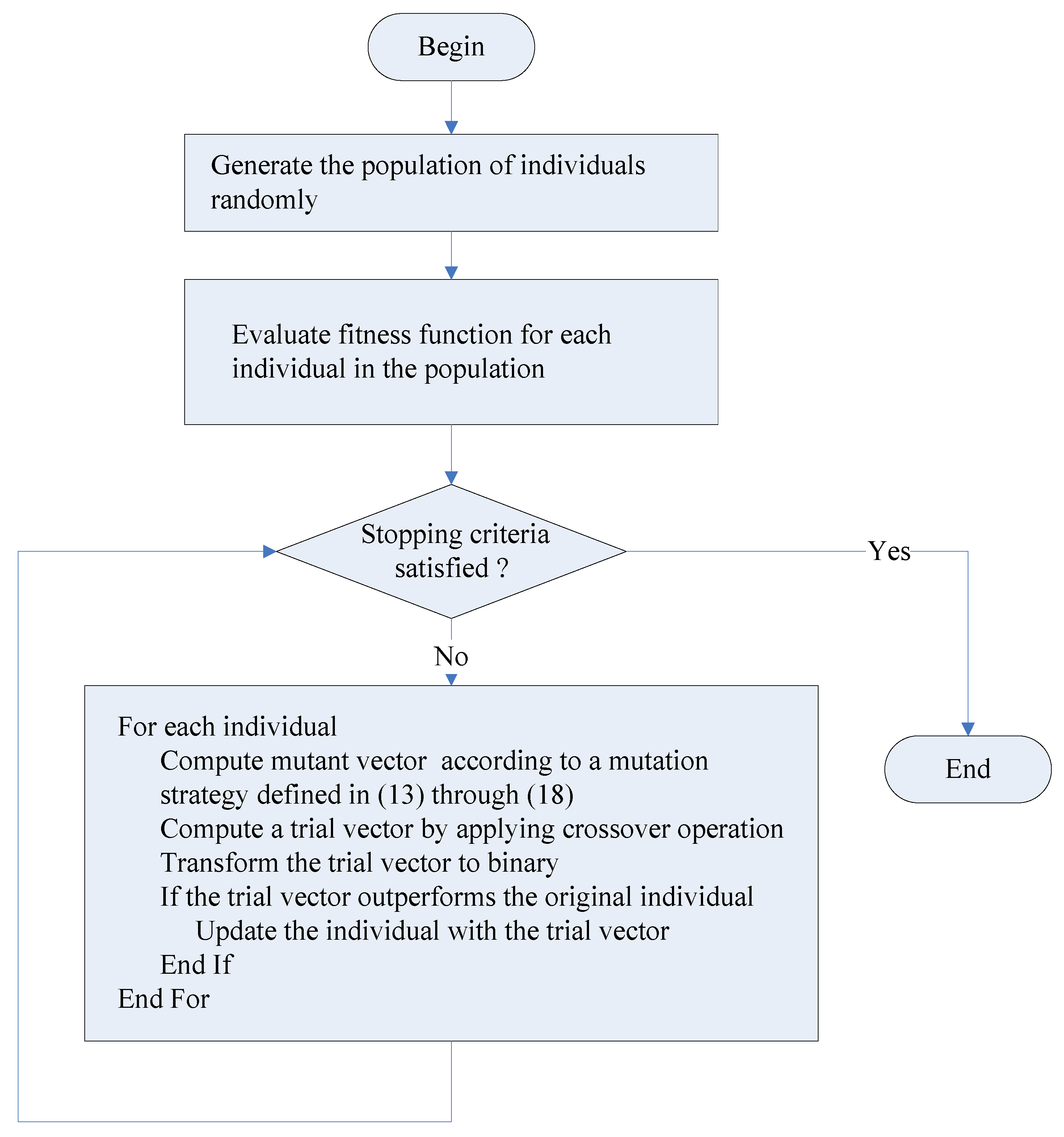
4.5. Discrete Differential Evolution Algorithm

There are three parameters in the DE algorithm, including scale factor, crossover rate and the number of individuals in the population (population size). To describe the DE algorithm, let $N$, $NP$, $CR$ and $F$ denote the problem dimension, population size, crossover rate and scale factor, respectively. The scale factor for individual $i$ is denoted by $F_i$. We use $t{v}_i$ to denote a mutant vector for individual $i$, where $i\in$ {1, 2, …, $NP$ }.

A DE algorithm starts by generating a random population of trial individuals $z_i=(z_{i1},z_{i2},z_{i3},\dots ,z_{iN})$ for $i$ = 1, 2, …, $NP$ and $n$ = 1, 2, …, $N$. The DE algorithm attempts to improve the quality of the trial populations. In each iteration, a new generation replaces the previous one. In the course of generating a new generation, a new mutant vector $t{v}_i=(t{v}_{i1},t{v}_{i2},t{v}_{i3},\dots ,t{v}_{iN})$ is generated for individual $z_i$ by applying a search strategy or mutation strategy, $S$. In existing literature, several search strategies have been proposed for DE. Six well-known search strategies in DE are as follows:

$$t{v}_{in}=z_{r_{1}n}+F_i(z_{r_{2}n}-z_{r_{3}n})$$

(13)

$$t{v}_{in}=z_{bn}+F_i(z_{r_{2}n}-z_{r_{3}n})$$

(14)

$$t{v}_{in}=z_{r_{1}n}+F_i(z_{r_{2}n}-z_{r_{3}n})+F_i(z_{r_{4}n}-z_{r_{5}n})$$

(15)

$$t{v}_{in}=z_{bn}+F_i(z_{r_{1}n}-z_{r_{2}n})+F_i(z_{r_{3}n}-z_{r_{4}n})$$

(16)

$$t{v}_{in}=z_{in}+F_i(z_{bn}-z_{in})+F_i(z_{r_{1}n}-z_{r_{2}n})$$

(17)

$$t{v}_{in}=z_{in}+F_i(z_{bn}-z_{in})+F_i(z_{r_{1}n}-z_{r_{2}n})+F_i(z_{r_{3}n}-z_{r_{4}n})$$

(18)

where the index $b$ refers to the best individual $z_b$.

Similarly, $z_{r_{1}n}$, $z_{r_{2}n}$, $z_{r_{3}n}$, $z_{r_{4}n}$ and $z_{r_{5}n}$ are some random individuals, namely, $r_1$, $r_2$, $r_3$, $r_4$ and $r_5$ are random integers between 1 and $NP$.

The standard DE algorithm was originally proposed to solve the problem in continuous search space. Therefore, it is necessary to transform each element of individual vector into one or zero in the discrete DE algorithm. The discrete DE algorithm can be described by a flowchart and a pseudocode. Figure 5 shows the flowchart for the discrete DE algorithm.

Table 8. The pseudocode for the discrete DE algorithm.

Discrete DE Algorithm

$t\leftarrow 0$ Set parameters $CR=0.5$ $F=N(0,1)$, where $N(0,1)$ is a Gaussian random variable with mean 0 and standard deviation 1.0 For $i=1toNP$   $F_i=F$ End For $S$: A mutation strategy defined in (13) through (18) Generate an initial population $S$ randomly While (stopping criteria not satisfied)   t ← t + 1   For $i=1toNP$     Compute mutant vector $v_i$     Compute $v_i$ according to mutation strategy $S$     Compute trial vector $u_i$ by crossover operation     For $n\in \{1,2,\dots ,N\}$      $u_{in}=\{\begin{array}{l}{v}_{in}ifRand(0,1)<CR\\ z_{in}otherwise\end{array}$     End For     Transform each element of $u_{in}$ into one or zero      ${\overline{u}}_{idg}\leftarrow CS(u_{idg})$     Update individual $i$      If $F_1({\overline{u}}_{ig})\ge F_1(z_{ig})$       $z_i$ = $u_i$      End If   End For End While

shows the pseudocode for the discrete DE algorithm.

5. Results

In this section, we conduct experiments by generating the data for several test cases and then apply four discrete variants of PSO algorithms, discrete variants of DE algorithms and the discrete firefly algorithm to find solutions for the test cases. First, we briefly introduce the data and parameters for test cases and the metaheuristic algorithms. We then compare different metaheuristic algorithms based on the results of experiments. The outputs obtained by applying different metaheuristic algorithms to each test case are summarized and analyzed in this section.

5.1. Data and Parameters

The input data are created by arbitrarily selecting a real geographical area first. Then, locations of drivers and passengers are randomly generated based on the selected geographical area. Therefore, the procedure for selecting input data is general and can be applied to other geographical areas in the real world. The test cases are generated based on a real geographical area in the central part of Taiwan. The data for each example are represented by bids. The data (bids) for these test cases are available for download from:

https://drive.google.com/drive/folders/1pl_bYMtWUCbGODYDmDr2aX2h_7WXSeNZ?usp=sharing.

To illustrate the elements of typical test cases’ data, the details of the data for a small example is introduced first.

An Example:

Consider a ridesharing system with one driver and four passengers. The origins and destinations of the driver and passengers are listed in

Table 9. Origins and destinations of participants.

Participant	Origin	Destination
Driver 1	24.13046 120.7047	24.2493791 120.6989202
Passenger 1	24.13745 120.68354	24.15294 120.65751
Passenger 2	24.17119 120.65015	24.13423 120.65639
Passenger 3	24.2033643 120.7047477	24.1344881 120.6674565
Passenger 4	24.2057 120.67951	24.2261 120.65644

.

Table 10. Bid submitted by Driver 1.

$\mathbf{Driver}\mathbf{ID}\left(\mathit{d}\right)$	${\mathit{q}}_{\mathit{d}11}$	${\mathit{q}}_{\mathit{d}12}$	${\mathit{q}}_{\mathit{d}13}$	${\mathit{q}}_{\mathit{d}14}$	${\mathit{o}}_{\mathit{d}1}$	${\mathit{c}}_{\mathit{d}1}$
1	1	0	0	0	55.4325	58.815

shows the bid generated for Driver 1 by applying the bid generation procedure in Appendix II of Reference [31]. The bids generated for all passengers are shown in

Table 11. Bids submitted by Passengers.

$\mathbf{Passenger}\mathbf{ID}\left(\mathit{p}\right)$	${\mathit{s}}_{\mathit{p}1}$	${\mathit{s}}_{\mathit{p}2}$	${\mathit{s}}_{\mathit{p}3}$	${\mathit{s}}_{\mathit{p}4}$	${\mathit{f}}_{\mathit{p}}$
1	1	0	0	0	11.8775
2	0	1	0	0	13.01
3	0	0	1	0	24.33
4	0	0	0	1	10.155

. Four discrete variants of PSO algorithms, six discrete variants of DE algorithms and the discrete firefly algorithm (FA) are applied to find solutions for this example. The parameters used for each metaheuristic algorithm in this study are as follows.

The parameters for the discrete CCPSO algorithm are:

• $DS$ = {2, 5, 10}
• ${\omega }_1$ = 0.5
• ${\omega }_2$ = 0.5
• $\theta$ = 1.0
• $V_{\max }$ = 4
• $MAX\_GEN$ = 10,000

The parameters for the discrete PSO algorithm are:

• $\omega$ = 0.4
• $c_1$ = 0.4
• $c_2$ = 0.6
• $V_{\max }$ = 4
• $MAX\_GEN$ = 10,000

The parameters for the firefly algorithm (FA) are:

• ${\beta }_0$ = 1.0
• $\gamma$ = 0.2
• $\alpha$ = 0.2
• $V_{\max }$ = 4
• $MAX\_GEN$ = 10,000

The parameters for the CLPSO algorithm are:

• $\omega$ = 0.4
• $c_1$ = 0.4
• $c_2$ = 0.6
• $p_c$ = 0.5
• $V_{\max }$ = 4
• $MAX\_GEN$ = 10,000

The parameters for the DE algorithm are:

• $CR$ = 0.5
• $F$: Gaussian random variable with zero mean and standard deviation set to 1.0
• $V_{\max }$ = 4
• $MAX\_GEN$ = 10,000
• Population size $NP$ = 10

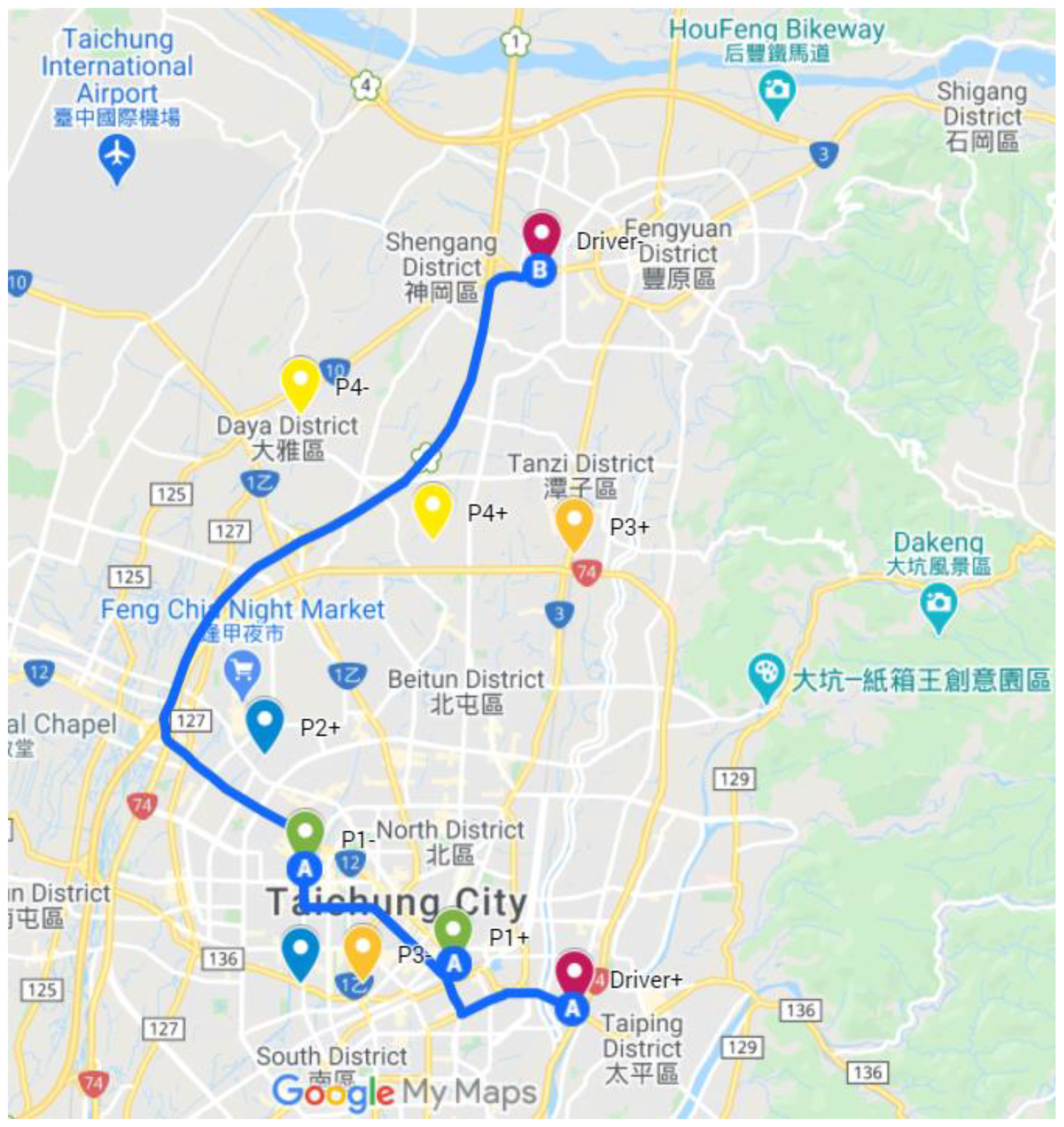
For this example, all the above algorithms obtain the same solution $x_{1,1}=1$, $y_{1,1}=1$, $y_{2,1}=0$, $y_{3,1}=0$, $y_{4,1}=0$. The solution indicates that Driver 1 will share a ride with Passenger 1 only to optimize monetary incentive. The objective function value for this solution is 0.12. Figure 6 shows the results on Google Maps.

5.2. Comparison of Different Metaheuristic Algorithms

Experiments for several test cases have been conducted to compare different metaheuristic algorithms. The parameters for running all the algorithms for Case 1 through Case 6 are the same as those used by the Example in Section 5.1, with the exception that the population size $NP$ is either set to 10 or 30. The parameters for running all the algorithms for Case 7 and Case 8 are the same as those used by the Example in Section 5.1, with the exception that the maximum number of generations $MAX\_GEN$ is set to 50,000 and the population size $NP$ is either set to 10 or 30. The results are as follows.

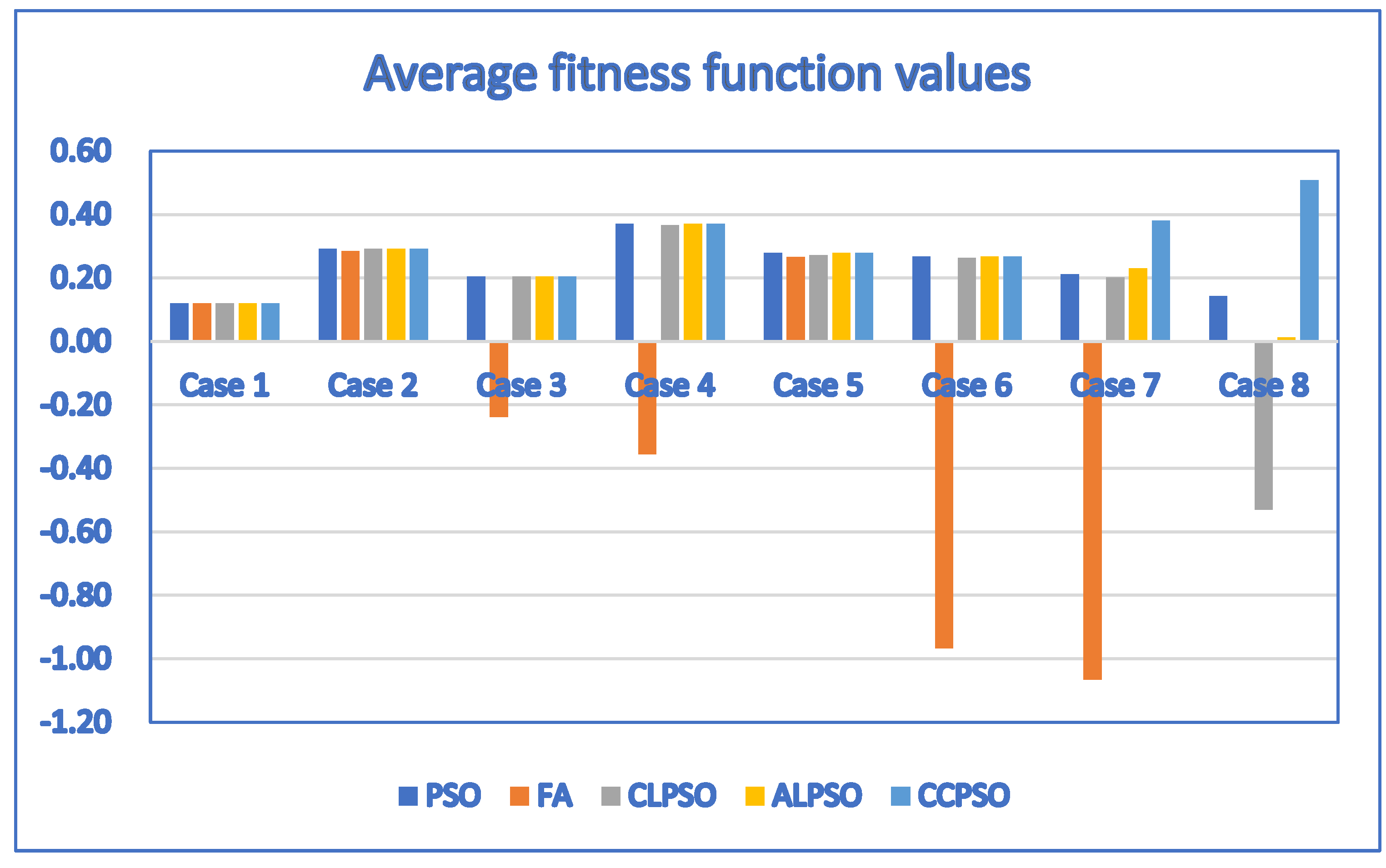
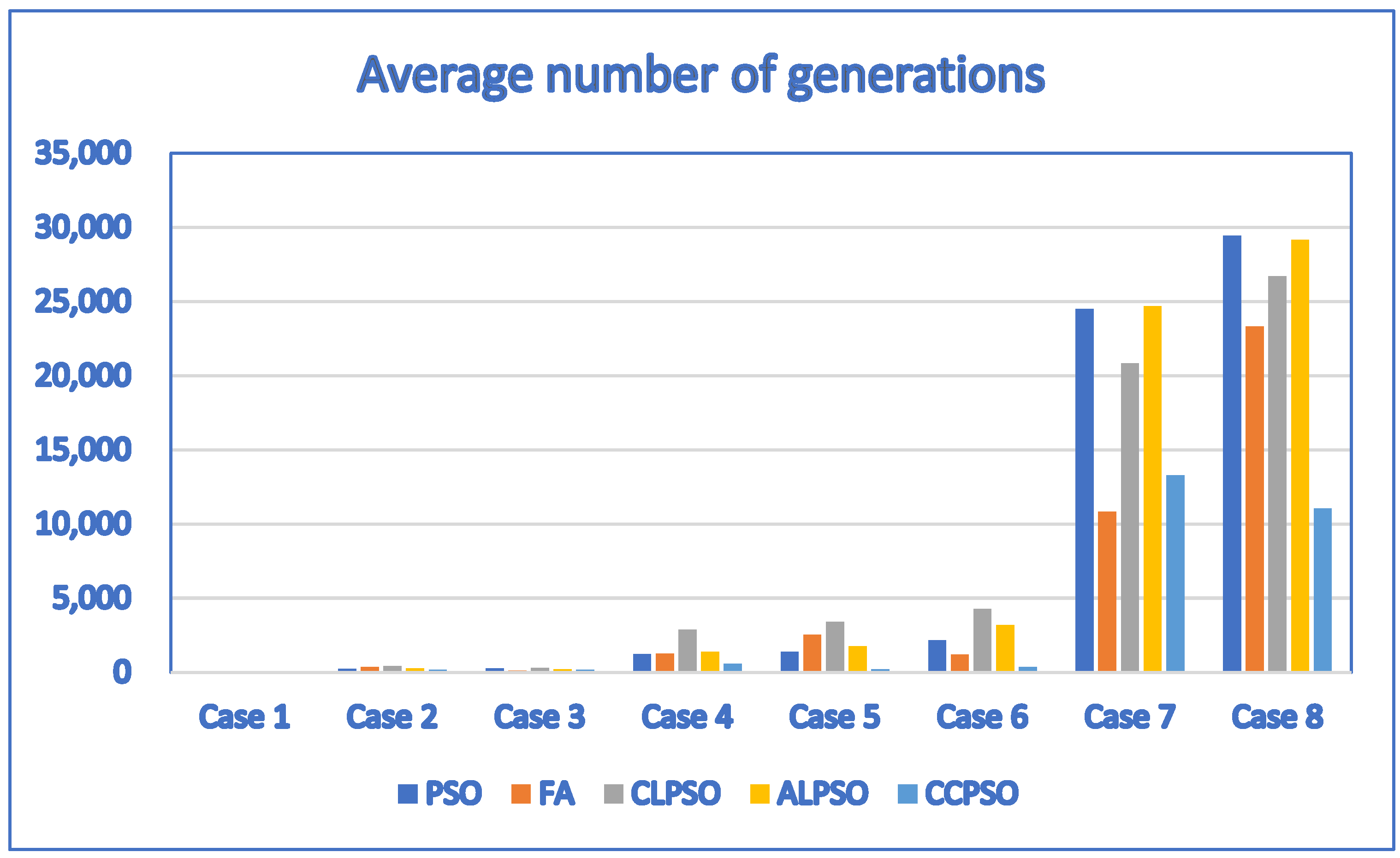
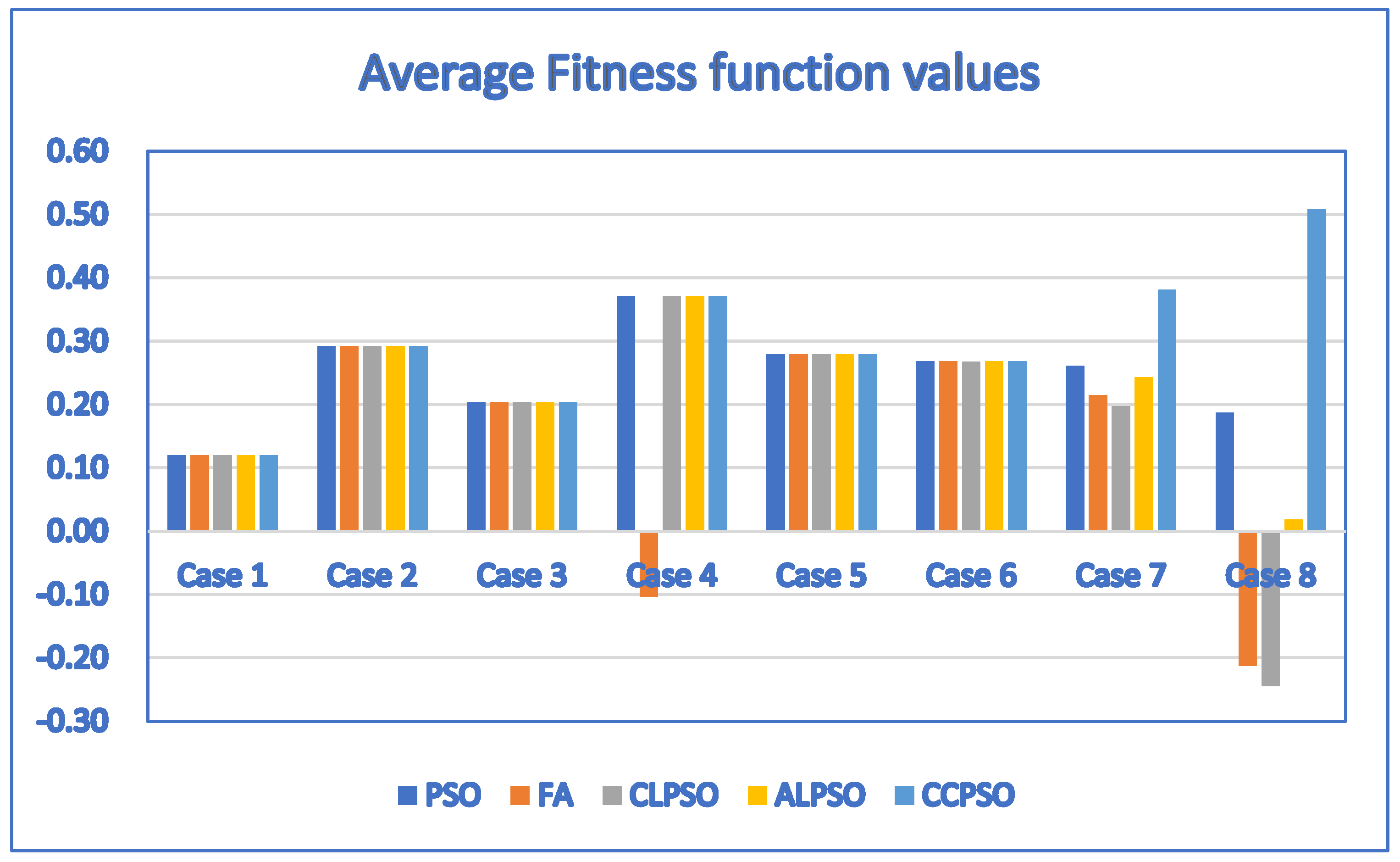
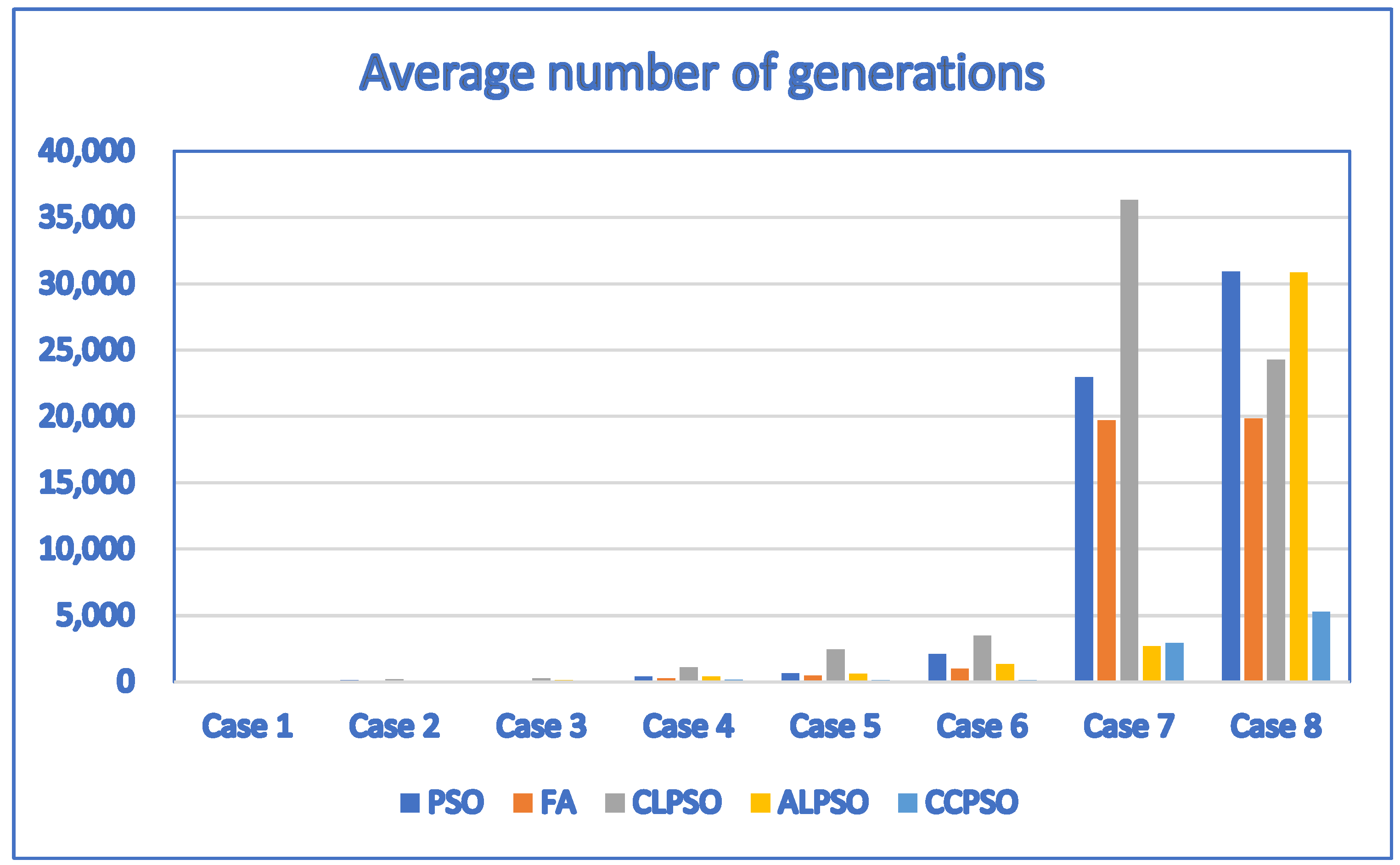
By setting the population size $NP$ to 10 and applying the discrete PSO, discrete firefly (FA), discrete ALPSO and discrete CCPSO algorithms to solve the problems, we obtained the results of

Table 12. Fitness function values for discrete PSO, CCPSO, CLPSO, ALPSO and FA algorithms (population size $NP$ = 10). Avg. = average.

Case	D	P	PSO	FA	CLPSO	ALPSO	CCPSO
			Avg. Fitness Value/Avg. Generation	Avg. Fitness Value/Avg. Generation	Avg. Fitness Value/Avg. Generation	Avg. Fitness Value/Avg. Generation	Avg. Fitness Value/Avg. Generation
1	1	4	0.12/3.2	0.12/4.6	0.12/3.1	0.12/3.3	0.12/3.9
2	3	10	0.292/216.4	0.2849/344	0.292/410.4	0.292/263.3	0.292/156.9
3	3	10	0.204/267.9	−0.2373/95.1	0.204/297.6	0.204/205.3	0.204/177.2
4	5	11	0.371/1222.1	−0.3558/1252.6	0.3667/2855.7	0.371/1365.6	0.371/568.7
5	5	12	0.279/1381.2	0.2663/2513.6	0.2721/3388.9	0.279/1756.5	0.279/184.4
6	6	12	0.268/2147.6	−0.9662/1195.2	0.2638/4282.2	0.2679/3187.1	0.268/364.5
7	20	20	0.2111/24,501	−1.0659/10,817.5	0.2023/20,843.7	0.2298/24,681	0.381/13,288.5
8	30	30	0.1423/29,449.2	−1.6923/23,324.6	−0.5304/26,707.3	0.0125/29,172	0.508/11,036.7

. It indicates that the discrete CCPSO algorithm outperforms the discrete firefly algorithm and discrete ALPSO algorithm. Although the average fitness function values of the discrete PSO algorithm and the discrete CCPSO algorithm are the same for small test cases (Case 1 through Case 6), the average number of generations needed by the discrete CCPSO algorithm is less than that of the discrete PSO algorithm for most test cases. In particular, the discrete CCPSO algorithm outperforms the discrete PSO algorithm in terms of the average fitness function values and the average number of generations needed for larger test cases (Case 7 and Case 8). This indicates that the discrete CCPSO algorithm outperforms the discrete PSO algorithm for most test cases when the population size $NP$ is 10.

For Table 12, the corresponding bar chart for the average fitness function values of discrete PSO, CCPSO, CLPSO, ALPSO and FA algorithms is shown in Figure 7.

For Table 12, the corresponding bar chart for the average number of generations of discrete PSO, CCPSO, CLPSO, ALPSO and FA algorithms is shown in Figure 8.

By setting the population size $NP$ to 10 and applying the discrete DE algorithm with six well-known strategies to solve the problems, we obtained

Table 13. Average (Avg.) fitness function values/generations for discrete DE algorithms with strategy 1, strategy 2 and strategy 3 (population size $NP$ = 10).

Case	D	P	DE_Strategy 1	DE_Strategy 2	DE_Strategy 3
			Avg. Fitness Value/Avg. Generation	Avg. Fitness Value/Avg. Generation	Avg. Fitness Value/Avg. Generation
1	1	4	0.12/3.1	0.12/4.4	0.12/2.3
2	3	10	0.292/86.7	0.281/574.8	0.292/102.7
3	3	10	0.1995/867	0.2023/180.2	0.1903/146.4
4	5	11	0.3389/220.5	0.2896/1027.4	0.3177/1179.6
5	5	12	0.2745/1914.2	0.2553/2233.4	0.2681/574
6	6	12	0.2542/417	0.2307/894.2	0.2521/541.3
7	20	20	0.2622/2764.4	0.1819/13,610.3	0.3266/6310.3
8	30	30	0.256/15,267.8	−0.0367/11,861.2	0.3258/10,241.7

and

Table 14. Average (Avg.) fitness function values/generations for discrete DE algorithms with strategy 4, strategy 5 and strategy 6 (population size $NP$ = 10).

Case	D	P	DE_Strategy 4	DE_Strategy 5	DE_Strategy 6
			Avg. Fitness Value/Avg. Generation	Avg. Fitness Value/Avg. Generation	Avg. Fitness Value/Avg. Generation
1	1	4	0.12/2.3	0.12/2.8	0.12/2.4
2	3	10	0.2834/79.9	0.2834/1867.6	0.2801/170.2
3	3	10	0.2017/63.3	0.202/1065.3	0.2031/475.8
4	5	11	0.3416/835.4	0.3536/1393.3	0.3263/1201.9
5	5	12	0.261/2318.2	0.2332/1491.5	0.2758/256.1
6	6	12	0.2606/219.1	0.2491/2854.4	0.2677/796.9
7	20	20	0.2219/9339.7	0.1898/14,519.7	0.0485/10,533.6
8	30	30	0.227/18,229.7	−0.0598/13,292.6	0.1072/20,699.7

. By comparing Table 13, Table 14 and Table 12, it indicates that the discrete CCPSO algorithm outperforms the discrete DE algorithm for most test cases. The discrete DE algorithm performs as good as the discrete CCPSO algorithm only for Test Case 1. For Test Case 2, only two DE strategies (Strategy 1 and Strategy 3) perform as good as the discrete CCPSO algorithm. The discrete CCPSO algorithm outperforms the discrete DE algorithm for Test Case 3 through Test Case 6. This indicates that the discrete CCPSO algorithm outperforms the discrete PSO algorithm when the population size $NP$ is 10.

For Table 13 and Table 14, the corresponding bar chart for the average fitness function values of discrete DE algorithms with strategy 1, strategy 2, strategy 3, strategy 4, strategy 5 and strategy 6 (population size = 10) is shown in Figure 9.

For Table 13 and Table 14, the corresponding bar chart for the average number of generations of discrete DE algorithms with strategy 1, strategy 2, strategy 3, strategy 4, strategy 5 and strategy 6 (population size = 10) is shown in Figure 10.

We obtained

Table 15. Average (Avg.) fitness function values/generations for discrete PSO, CCPSO, CLPSO, ALPSO and FA algorithms (population size $NP$ = 30).

Case	D	P	PSO	FA	CLPSO	ALPSO	CCPSO
			Avg. Fitness Value/Avg. Generation	Avg. Fitness Value/Avg. Generation	Avg. Fitness Value/Avg. Generation	Avg. Fitness Value/Avg. Generation	Avg. Fitness Value/Avg. Generation
1	1	4	0.12/2.1	0.12/2	0.12/2.3	0.12/2.1	0.12/2.4
2	3	10	0.292/114.7	0.292/34.7	0.292/176.3	0.292/65.3	0.292/40.1
3	3	10	0.204/69.6	0.204/29	0.204/241.1	0.204/118.4	0.204/84.2
4	5	11	0.371/371.7	−0.1032/236.4	0.371/1074.1	0.371/383.4	0.371/141.8
5	5	12	0.279/619.8	0.279/450.5	0.279/2424.8	0.279/586.9	0.279/93.8
6	6	12	0.268/2090.9	0.268/958.8	0.2678/3479.7	0.268/1325.2	0.268/116.8
7	20	20	0.2609/22,957.7	0.2149/19,716.8	0.1971/36,331.3	0.2432/2663.7	0.381/2909.8
8	30	30	0.1875/30,923.7	−0.213/19,855.3	−0.2449/24,290.3	0.1811/30,853.2	0.508/5266.9

by applying the discrete PSO, the discrete firefly, the discrete CLPSO, discrete ALPSO and discrete CCPSO algorithms to solve the problems with population size $NP=30$. Table 15 indicates that the average fitness function values found by the discrete PSO, discrete ALPSO and discrete CCPSO algorithms are the same for small test cases (Test Case 1 through Test Case 6). The results indicate that the discrete PSO, discrete ALPSO and discrete CCPSO algorithms outperform the discrete FA and discrete CLPSO algorithms for small test cases (Test Case 1 through Test Case 6). The discrete CCPSO algorithm outperforms the discrete PSO, the discrete FA, the discrete CLPSO and the discrete ALPSO algorithms for larger test cases (Test Case 7 and Test Case 8). The discrete CCPSO algorithm does not just outperform the discrete PSO, the discrete FA, the discrete CLPSO and the discrete ALPSO algorithms in terms of the average fitness function values found, also, the average numbers of generations needed by the discrete CCPSO algorithm to find the best solutions are less than those of the discrete PSO algorithm and the discrete ALPSO algorithm for most test cases. This indicates that the discrete CCPSO algorithm is more efficient than the discrete PSO, the discrete FA, the discrete CLPSO and the discrete ALPSO algorithms for most test cases when the population size $NP$ is 30.

For Table 15, the corresponding bar chart for the average number of generations of discrete PSO, CCPSO, CLPSO, ALPSO and firefly (FA) algorithms is shown in Figure 11.

For Table 15, the corresponding bar chart for the average number of generations of discrete PSO, CCPSO, CLPSO, ALPSO and FA algorithms is shown in Figure 12.

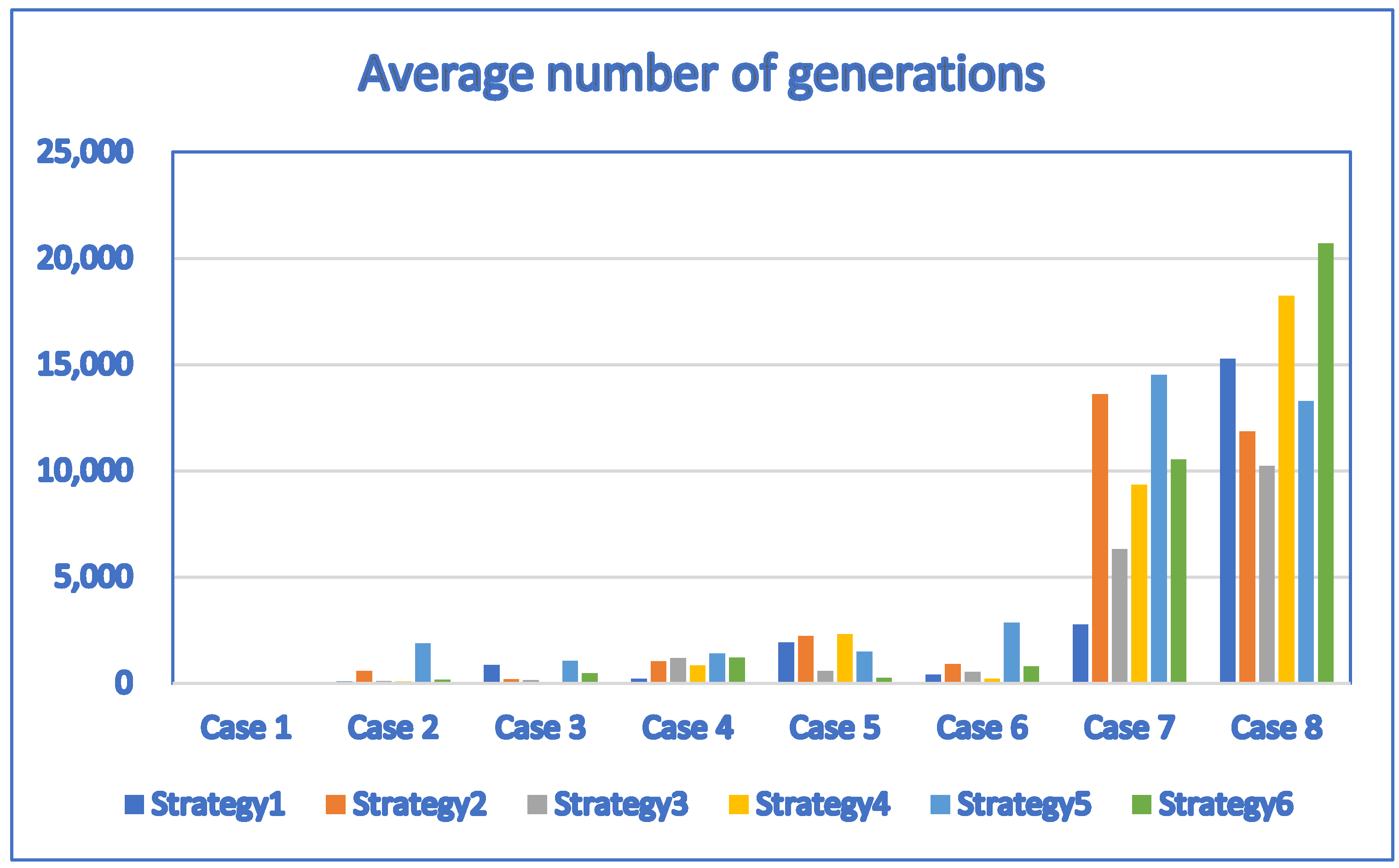
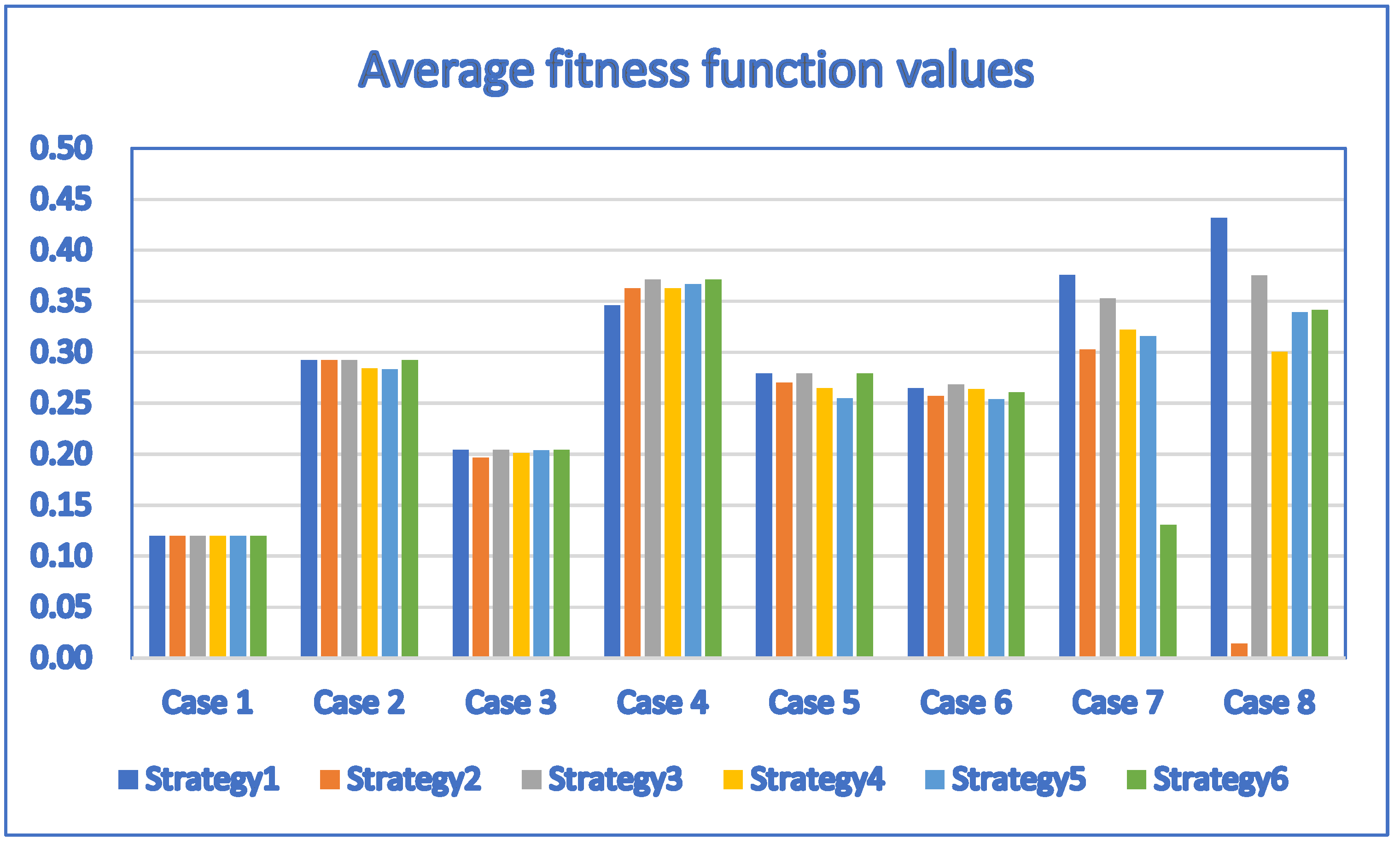
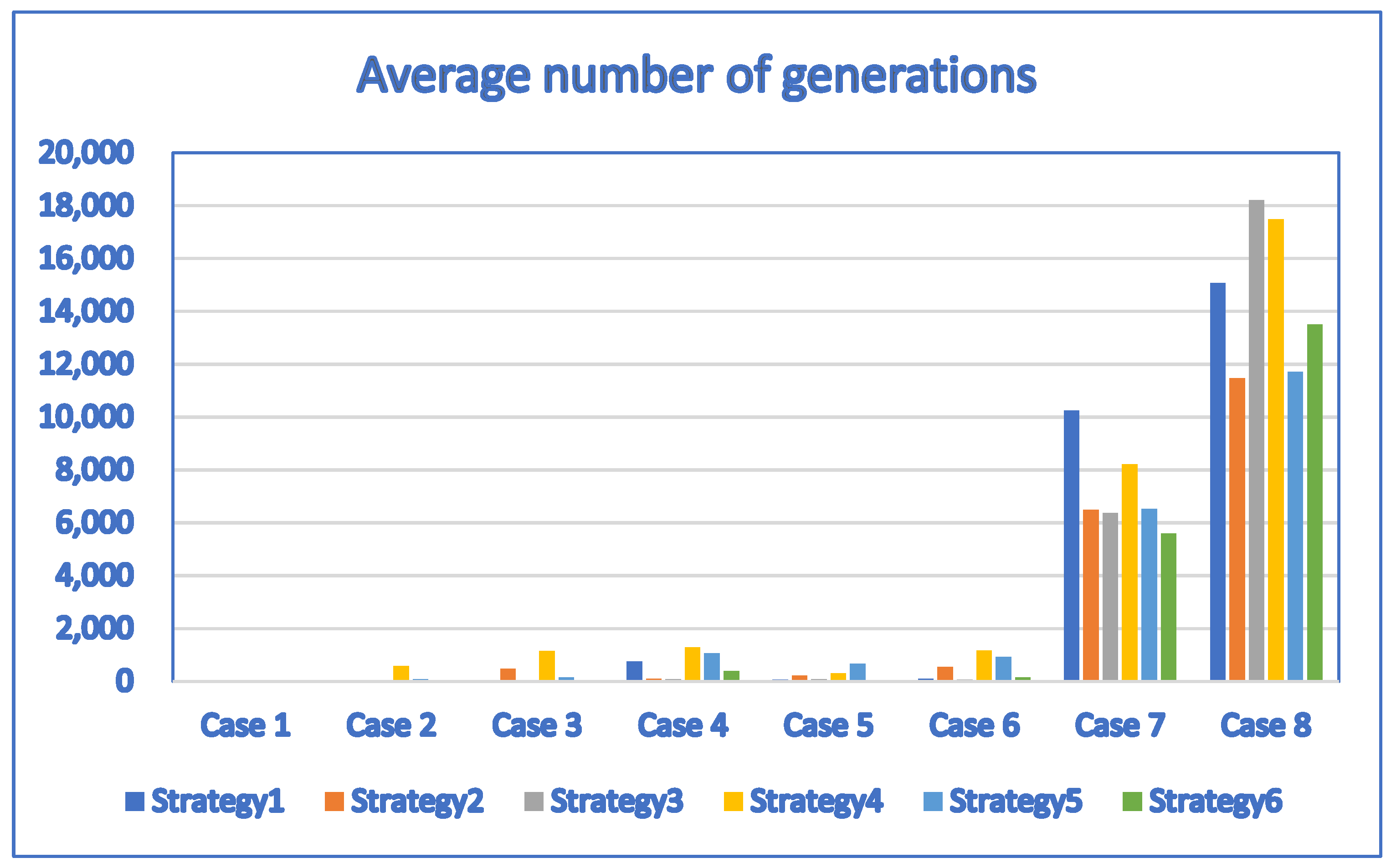
We obtained

Table 16. Average (Avg.) fitness function values/generations for discrete DE algorithms with strategy 1, strategy 2 and strategy 3 (population size $NP$ = 30).

Case	D	P	DE_Strategy1	DE_Strategy2	DE_Strategy3
			Avg. Fitness Value/Avg. Generation	Avg. Fitness Value/Avg. Generation	Avg. Fitness Value/Avg. Generation
1	1	4	0.12/1.2	0.12/1.5	0.12/1.6
2	3	10	0.292/22.5	0.292/25.875	0.292/25.625
3	3	10	0.204/22.3	0.1966/478.3	0.204/30.7
4	5	11	0.3458/756.7	0.3624/94.8	0.371/79.9
5	5	12	0.279/66.4	0.27/216.2	0.279/88.5
6	6	12	0.2646/97.2	0.2571/548.8	0.268/76.9
7	20	20	0.3758/10,239	0.3027/6492.6	0.3528/6385.7
8	30	30	0.4316/15,061.3	0.0142/11,460	0.3754/18,206.9

and

Table 17. Average (Avg.) fitness function values/generations for discrete DE algorithms with strategy 4, strategy 5 and strategy 3 (population size $NP$ = 30).

Case	D	P	DE_Strategy4	DE_Strategy5	DE_Strategy6
			Avg. Fitness Value/Avg. Generation	Avg. Fitness Value/Avg. Generation	Avg. Fitness Value/Avg. Generation
1	1	4	0.12/1.5	0.12/1.1	0.12/1.5
2	3	10	0.28425/577.375	0.283/88.75	0.292/16.123
3	3	10	0.2011/1162.5	0.2035/160	0.204/30.9
4	5	11	0.3624/1290.4	0.3667/1063	0.371/395.9
5	5	12	0.2647/310.9	0.2546/667.8	0.279/38.7
6	6	12	0.2637/1179.8	0.2538/922.4	0.2607/160.4
7	20	20	0.3218/8211.2	0.3157/6530.8	0.1311/5601.5
8	30	30	0.3003/17,476.7	0.3393/11,709.7	0.3413/13,503.9

by setting the population size $NP$ to 30 and applying the discrete DE algorithm with six well-known strategies to solve the problems. Table 16 and Table 17 indicate that the performance of the discrete DE algorithm is improved for most test cases. For example, the average fitness function values obtained by the discrete DE algorithm with Strategy 3 are the same as those obtained by the discrete PSO, discrete ALPSO and discrete CCPSO algorithms for small test cases (Test Case 1 through Test Case 6). Although the average fitness function values obtained by the discrete DE algorithm with other strategies are no greater than those obtained by the discrete PSO, discrete ALPSO and discrete CCPSO algorithms, the performance of the discrete DE algorithm are close to the discrete PSO, discrete ALPSO and discrete CCPSO algorithms. The discrete CCPSO algorithm still outperforms the discrete DE algorithm with any of the six strategies for larger test cases (Test Case 7 and Test Case 8). Note that the average number of generations needed by the discrete DE algorithm to find the best solutions is significantly reduced for all strategies for most test cases. This indicates that the discrete DE algorithm works more efficiently for larger population size.

For Table 16 and Table 17, the corresponding bar chart for the average fitness function values of discrete DE algorithms with strategy 1, strategy 2, strategy 3, strategy 4, strategy 5 and strategy 6 (population size = 30) is shown in Figure 13.

For Table 16 and Table 17, the corresponding bar chart for the average number of generations of discrete DE algorithms with strategy 1, strategy 2, strategy 3, strategy 4, strategy 5 and strategy 6 (population size = 30) is shown in Figure 14.

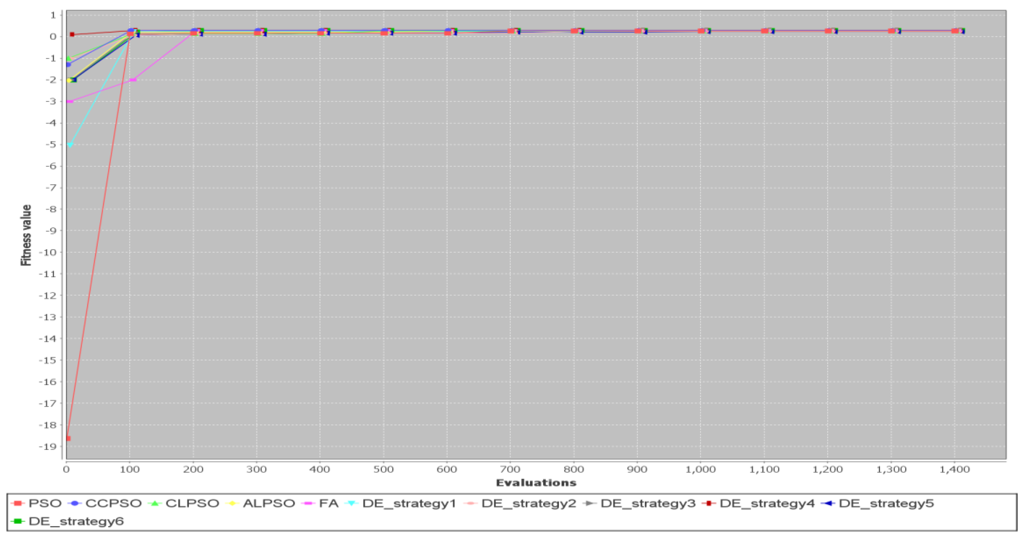
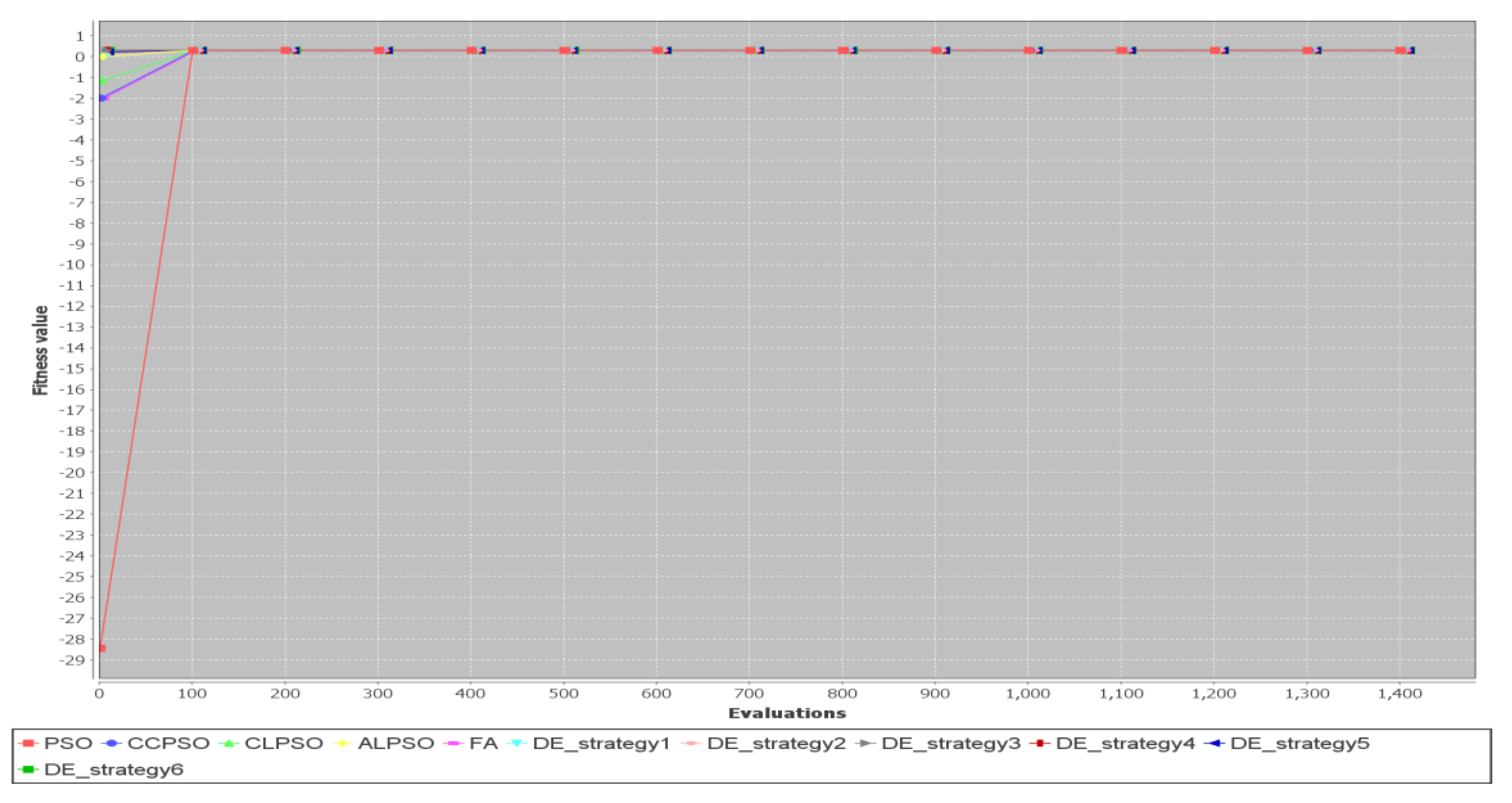
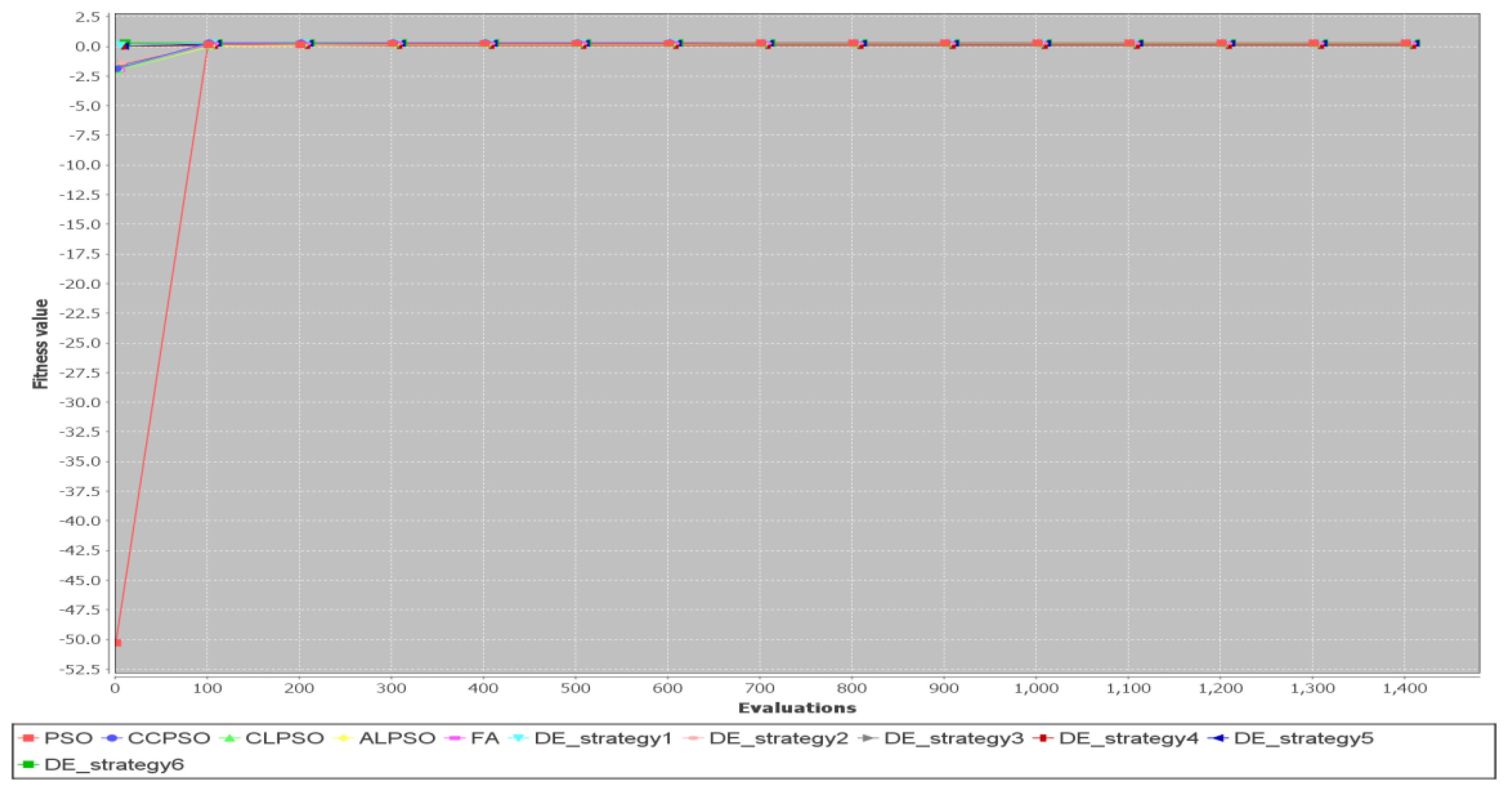
To study the convergence speed of the discrete PSO, discrete CLPSO, discrete ALPSO, discrete DE and discrete FA algorithms, we compare the convergence curves of simulation runs for several test cases. Figure 15 shows convergence curves for Test Case 2 ($NP$ = 10).

It indicates that the FA performs the worst for this simulation run. For this simulation run, the PSO algorithm converges the fastest. The CCPSO algorithm, the CLPSO algorithm, the ALPSO algorithm, the DE algorithm with Strategy 1, the DE algorithm with Strategy 3 and the DE algorithm with Strategy 6 also converge to the best fitness values very fast. The slowest algorithms are the firefly algorithm, the DE algorithm with Strategy 4 and the DE algorithm with Strategy 5.

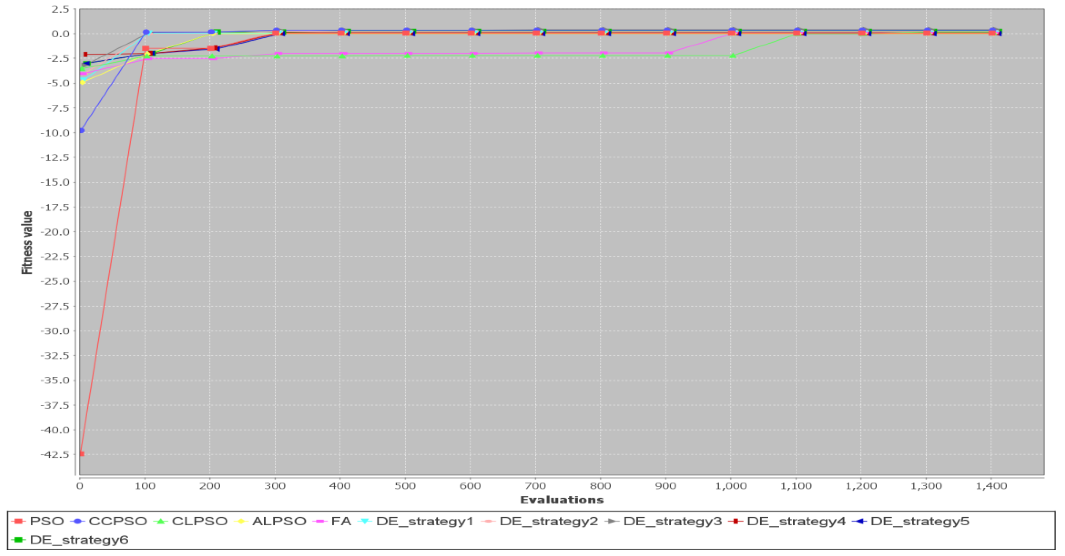
Figure 16 shows convergence curves for Test Case 5 ($NP$ = 10). Again, FA is the slowest among all the algorithms for this simulation run.

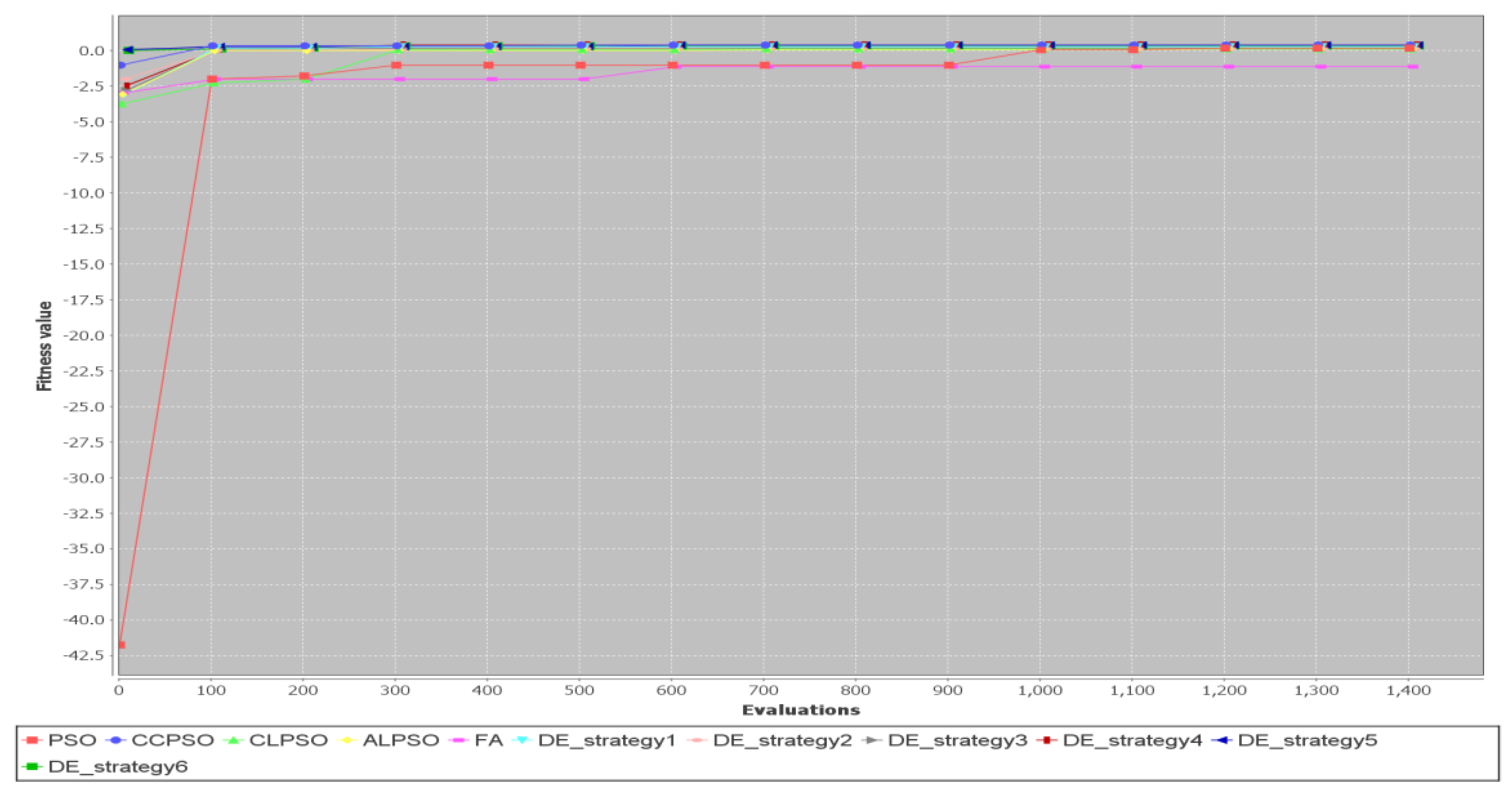
Figure 17 shows convergence curves for Test Case 7 ($NP$ = 10). FA and the CLPSO algorithms are the two slowest algorithms in terms of convergence rate.

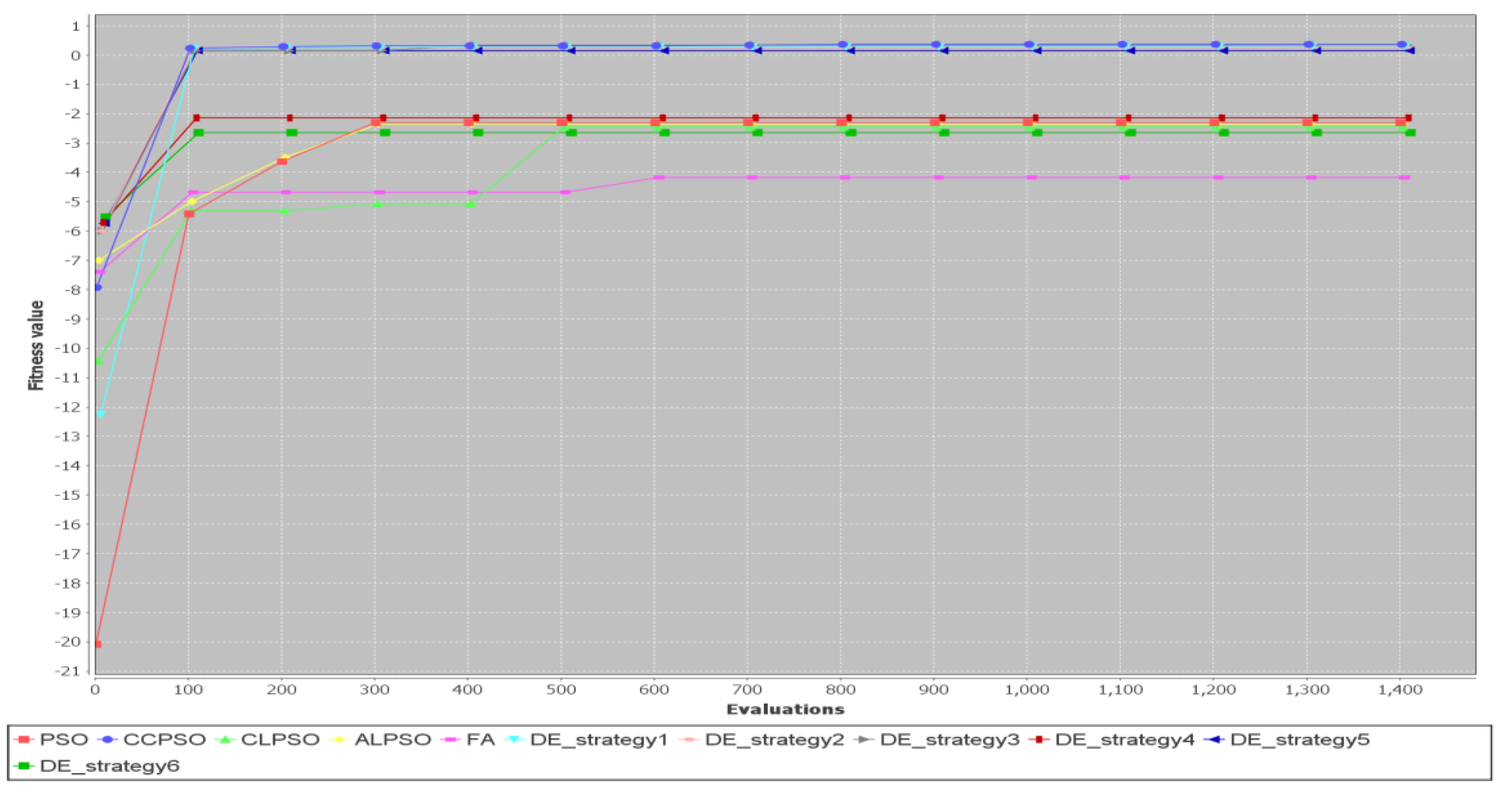
Figure 18 shows convergence curves for Test Case 8 ($NP$ = 10). The CCPSO algorithm and the DE algorithm with Strategy 1 are the fastest to converge to the best fitness values. All the other algorithms fail to converge to the best values.

Figure 19 shows convergence curves for Test Case 2 ($NP$ = 30). All algorithms converge very fast to the best solution in this simulation run for Test Case 2 when population size $NP$ = 30.

Figure 20 shows convergence curves for Test Case 5 ($NP$ = 30). All algorithms converge very fast to the best solution in this simulation run for Test Case 5 when population size $NP$ = 30.

For larger test cases, depending on the algorithm used, the convergence speed varies significantly. Figure 21 shows convergence curves for Test Case 7 ($NP$ = 30). The two fastest algorithms are the CCPSO algorithm and the DE algorithm with Strategy 6. In this run, the firefly algorithm is the slowest one and fails to converge to the best fitness value.

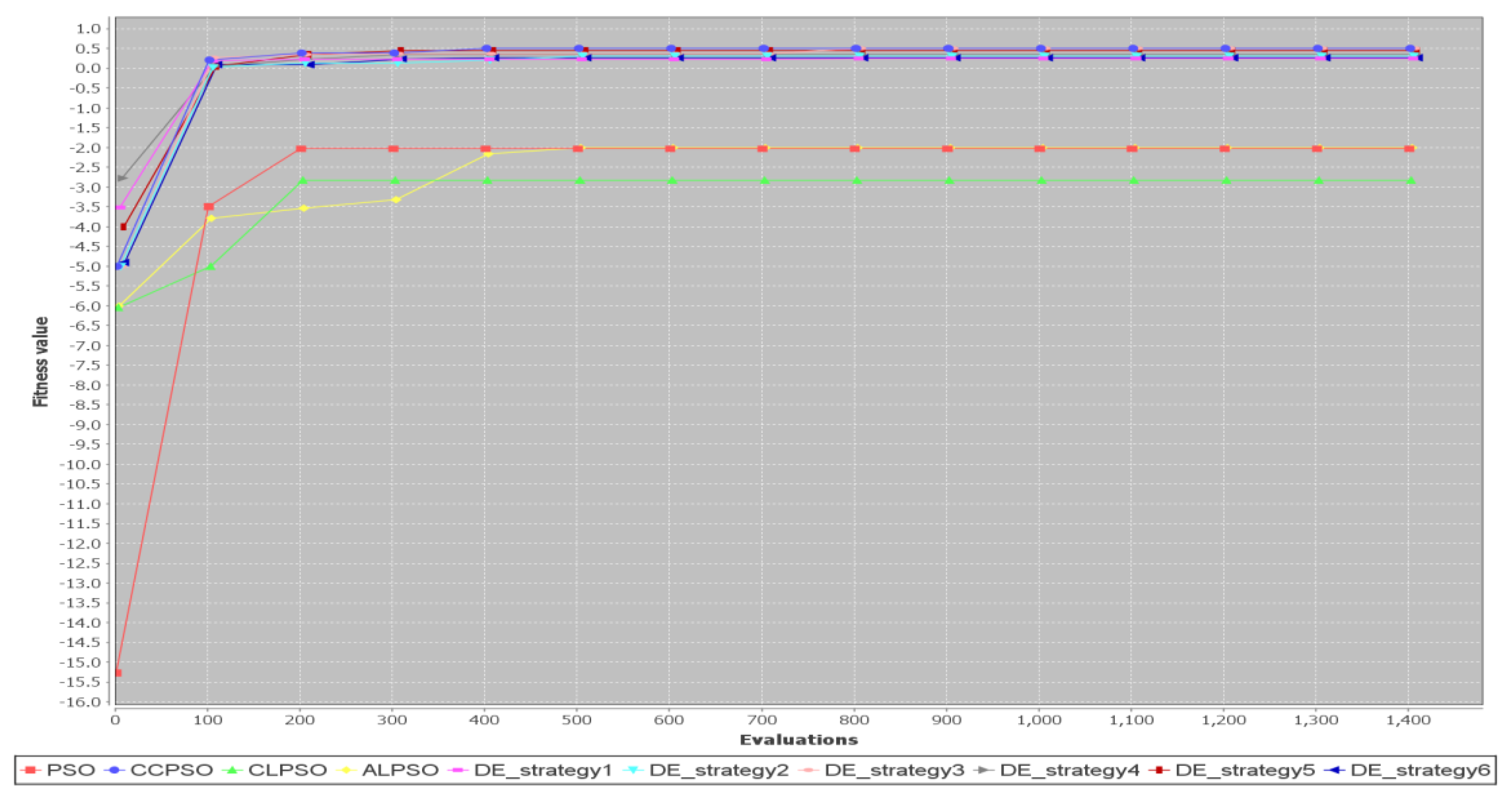
The variation in convergence speed is significant for another larger test case, Test Case 8. Figure 22 shows convergence curves for Test Case 8 ($NP$ = 30). The fastest algorithm is the CCPSO algorithm. In this run, the slowest algorithms are the PSO, CLPSO, ALPSO and FA. Note that the CLPSO, ALPSO and FA fail to converge to the best fitness value.

The results presented above indicate that the proposed discrete CCPSO algorithm outperforms other metaheuristic algorithms. Superiority of the discrete CCPSO algorithm is due to its capability to balance exploration and exploitation in the evolution processes. According to (11), $S{W}_s.z_{id}$ is updated with a Gaussian random variable $\mathrm{N}({\omega }_{1}S{W}_s.z_i^p+{\omega }_{2}S{W}_s.\widehat{z},{\left(\theta \left|S{W}_s.z_i^p-S{W}_s.\widehat{z}\right|\right)}^2)$. Exploration and exploitation characteristics of the discrete CCPSO algorithm strongly depend on the magnitude $\left|S{W}_s.z_i^p-S{W}_s.\widehat{z}\right|$. The balance between exploration and exploitation of the discrete CCPSO is as follows: As long as the personal best of a particle is not the same as the global best, the magnitude $\left|S{W}_s.z_i^p-S{W}_s.\widehat{z}\right|$ is nonzero. In this case, the variance of the Gaussian random variable $\mathrm{N}({\omega }_{1}S{W}_s.z_i^p+{\omega }_{2}S{W}_s.\widehat{z},{\left(\theta \left|S{W}_s.z_i^p-S{W}_s.\widehat{z}\right|\right)}^2)$ will be nonzero. If the magnitude $\left|S{W}_s.z_i^p-S{W}_s.\widehat{z}\right|$ is large, the variance of the Gaussian random variable $\mathrm{N}({\omega }_{1}S{W}_s.z_i^p+{\omega }_{2}S{W}_s.\widehat{z},{\left(\theta \left|S{W}_s.z_i^p-S{W}_s.\widehat{z}\right|\right)}^2)$ will be large. This makes it possible to search a larger region around ${\omega }_{1}S{W}_s.z_i^p+{\omega }_{2}S{W}_s.\widehat{z}$. If the personal best of a particle is close to the global best, the magnitude $\left|S{W}_s.z_i^p-S{W}_s.\widehat{z}\right|$ will be small. In this case, the variance of the Gaussian random variable $\mathrm{N}({\omega }_{1}S{W}_s.z_i^p+{\omega }_{2}S{W}_s.\widehat{z},{\left(\theta \left|S{W}_s.z_i^p-S{W}_s.\widehat{z}\right|\right)}^2)$ tends to be small. This leads to a very small search region. Therefore, exploration and exploitation characteristics of the discrete CCPSO algorithm are balanced automatically in the solution searching process through the magnitude $\left|S{W}_s.z_i^p-S{W}_s.\widehat{z}\right|$.

Although the subject of ridesharing/carpooling has been studied for over a decade, it is still not in widespread use. Motivated by this fact, several papers attempt to identify factors that contribute to ridesharing/carpooling [12,13,14]. Waerden et al. investigated factors that stimulate people to change from car drivers to carpooling. They identified several attributes that may influence the attractiveness of carpooling, including flexibility/uncertainty in travel time, costs and number of persons [13]. Their study indicates that the most influential are costs and time-related attributes in carpooling. Delhomme and Gheorghiu investigated the socio-demographics and transportation accessibility factual data to study motivational factors that differentiate carpoolers from non-carpoolers and highlight the main determinants of carpooling [12]. Their study indicates that the main incentives for carpooling are financial gains, time savings and environmental protection. Shaheen et al. studied a special type of carpooling called casual carpooling, which provides participants the benefits through access to a high-occupancy vehicle lane with tolling discounts. The study of Shaheen et al. indicates that monetary savings and time savings are the main motivations for casual carpooling participation [14].

Santos and Xavier [15] studied the ridesharing problem in which money is considered as an incentive. The study by Watel and Faye [16] focuses on a taxi-sharing problem, called Dial-a-Ride problem with money as an incentive (DARP-M). They studied the taxi-sharing problem to reduce the cost of passengers. Watel and Faye defined three variants of the DARP-M problem: max-DARP-M, max-1-DARP-M and 1-DARP-M, to analyze their complexity. The objective of max-DARP-M is to drive the maximum number of passengers under the assumption of unlimited number of taxis available. The max-1-DARP-M problem is used to find the maximum number of passenger that can be transported by a taxi. The 1-DARP-M problem is used to decide whether it is possible to drive at least one passenger under the constraints stated. Although the max-DARP-M, max-1-DARP-M and 1-DARP-M problems can be used to analyze complexity, they do not reflect real application scenarios. In addition, the problem to optimize overall monetary incentive is not addressed in References [15] and [16]. In Reference [17], Hsieh considered a monetary incentive in ridesharing systems and proposed a PSO-based solution algorithm for it. However, there is still lack of study on comparison with other variants of metaheuristic algorithms for solving the monetary incentive optimization problem formulated in this study. The results presented in this study serve to compare the effectiveness of applying several different metaheuristic algorithms to solve the monetary incentive optimization problem. The effectiveness of applying metaheuristic algorithms to solving a problem is assessed by performance and efficiency. Performance is reflected in the average number of fitness function values found by the metaheuristic algorithm applied, whereas efficiency is measured by the average number of generations needed to find the best fitness function values in the simulation runs. In this study, the comparative study on performance and efficiency was helpful for assessing the effectiveness of applying these metaheuristic approaches to solve the monetary incentive optimization problem.

6. Conclusions

Motivated by the fact that the performance indices considered in most studies on ridesharing are not directly linked to monetary incentive, this study focused on how to deal with the monetary incentive issue in ridesharing systems to promote the ridesharing transportation model. This study contributes to the literature by (1) proposing a monetary incentive performance index, (2) formulating a monetary incentive optimization problem formulation, (3) developing solution algorithms based on several metaheuristic approaches to find drivers and passengers with the highest monetary incentive for ridesharing and (4) providing a guideline for selecting a proper metaheuristic algorithm to solve the problem through comparing the effectiveness of several metaheuristic algorithms.

As the performance indicator for this problem is a highly non-linear and non-separable function and the decision variables are discrete, the optimization problem is a non-linear integer programming problem. It is computationally complex to find the solutions for this problem. To cope with computational complexity, metaheuristic approaches were adopted to solve the problem. Several discrete algorithms have been developed based on variants of PSO, DE and the firefly algorithms. To assess the effectiveness of these proposed algorithms, experiments for several test cases were conducted. The results show that the discrete CCPSO algorithm outperformed the variants discrete PSO algorithms, DE algorithm and the firefly algorithm when the population size was 10 or 30. The average fitness function values obtained by applying the discrete PSO algorithm were the same as those obtained by the discrete CCPSO algorithm for small test cases when the population size was 10. But, the average number of generations needed by the discrete CCPSO algorithm was less than those of the discrete PSO algorithm for most test cases. This indicates that the discrete CCPSO algorithm outperformed the discrete PSO algorithm when the population size was 10. The effectiveness of the variants of DE algorithms were significantly improved when the population size was increased to 30. The variants of DE algorithms were competitive with the discrete CCPSO algorithm in terms of performance and efficiency when the population size was increased. However, the variants of DE algorithms were more sensitive to population size in comparison with the discrete CCPSO algorithm. The discrete CCPSO algorithm worked effectively even if the population size was 10. These results provide guidelines for selecting metaheuristic algorithms to solve the monetary incentive optimization problem. The results indicate that many metaheuristic algorithms perform poorly as the problem grows due to premature convergence and/or the complex structure of constraints in the optimization problem, although they can be applied to develop solution algorithms for the nonlinear integer programming problem. The cooperative coevolution approach copes with these shortcomings of metaheuristic algorithms.

An interesting future research direction is to develop new methods to study the sensitivity with respect to algorithmic parameters of metaheuristic algorithms such as the population size. As the results indicate that the discrete CCPSO algorithm can solve non-linear integer programming problems effectively, another future research direction is to study whether the proposed discrete CCPSO algorithm can effectively deal with an integer programming problem with non-linear objective function and non-linear constraints. The first step to carry out this future research direction is to identify the optimization problem with non-linear objective function and non-linear constraints to pave the way for extending the proposed discrete CCPSO algorithm to general non-linear integer programming problems. The second step is to develop a method for handling non-linear constraints.

References

- Furuhata, M.; Dessouky, M.; Ordóñez, F.; Brunet, M.; Wang, X.; Koenig, S. Ridesharing: The state-of-the-art and future directions. Transp. Res. Pt. B-Methodol. 2013, 57, 28–46. [Google Scholar] [CrossRef]
- Agatz, N.; Erera, A.; Savelsbergh, M.; Wang, X. Optimization for dynamic ride-sharing: A review. Eur. J. Oper. Res. 2012, 223, 295–303. [Google Scholar] [CrossRef]
- Genikomsakis, K.N.; Ioakimidis, C.S.; Bocquier, B.; Savvidis, D.; Simic, D. Electromobility and carsharing/carpooling services at the University of Deusto: A preliminary exploratory survey. In Proceedings of the 16th International IEEE Conference on Intelligent Transportation Systems (ITSC 2013), The Hague, The Netherlands, 6–9 October 2013; pp. 1935–1940. [Google Scholar]
- Bruglieri, M.; Ciccarelli, D.; Colorni, A.; Luè, A. PoliUniPool: A carpooling system for universities. Procedia Soc. Behav. Sci. 2011, 20, 558–567. [Google Scholar] [CrossRef] [Green Version]
- Baldacci, R.; Maniezzo, V.; Mingozzi, A. An Exact Method for the Car Pooling Problem Based on Lagrangean Column Generation. Oper. Res. 2004, 52, 422–439. [Google Scholar] [CrossRef]
- Maniezzo, V.; Carbonaro, A.; Hildmann, H. An ants heuristic for the long-term car pooling problem. In New Optimization Techniques in Engineering; Onwubolu, G., Babu, B.V., Eds.; Springer: Berlin/Heidelberg, Germany, 2004; Volume 141, pp. 411–430. [Google Scholar]
- Agatz, N.A.H.; Erera, A.L.; Savelsbergh, M.W.P.; Wang, X. Dynamic ride-sharing: A simulation study in metro Atlanta. Transp. Res. Pt. B-Methodol. 2011, 45, 1450–1464. [Google Scholar] [CrossRef]
- Bicocchi, N.; Mamei, M. Investigating ride sharing opportunities through mobility data analysis. Pervasive Mob. Comput. 2014, 14, 83–94. [Google Scholar] [CrossRef]
- Toader, B.; Sprumont, F.; Faye, S.; Popescu, M.; Viti, F. Usage of Smartphone Data to Derive an Indicator for Collaborative Mobility between Individuals. ISPRS Int. J. Geo-Inf. 2017, 6, 62. [Google Scholar] [CrossRef] [Green Version]
- Hsieh, F.S. Car Pooling Based on Trajectories of Drivers and Requirements of Passengers. In Proceedings of the 2017 IEEE 31st International Conference on Advanced Information Networking and Applications (AINA 2017), Taipei, Taiwan, 27–29 March 2017; pp. 972–978. [Google Scholar]
- Bian, Z.; Liu, X.; Bai, Y. Mechanism design for on-demand first-mile ridesharing. Transp. Res. Pt. B-Methodol. 2020, 138, 77–117. [Google Scholar] [CrossRef]
- Delhomme, P.; Gheorghiu, A. Comparing French carpoolers and non-carpoolers: Which factors contribute the most to carpooling? Transport. Res. Part D-Transport. Environ. 2016, 42, 1–115. [Google Scholar] [CrossRef]
- Waerden, P.; Lem, A.; Schaefer, W. Investigation of Factors that Stimulate Car Drivers to Change from Car to Carpooling in City Center Oriented Work Trips. Transp. Res. Procedia 2015, 10, 335–344. [Google Scholar] [CrossRef] [Green Version]
- Shaheen, S.A.; Chan, N.D.; Gaynor, T. Casual carpooling in the San Francisco Bay Area: Understanding user characteristics, behaviors, and motivations. Transp. Policy 2016, 51, 165–173. [Google Scholar] [CrossRef] [Green Version]
- Santos, D.O.; Xavier, E.C. Taxi and Ride Sharing: A Dynamic Dial-a-Ride Problem with Money as an Incentive. Expert Syst. Appl. 2015, 42, 6728–6737. [Google Scholar] [CrossRef]
- Watel, D.; Faye, A. Taxi-sharing: Parameterized complexity and approximability of the dial-a-ride problem with money as an incentive. Theor. Comput. Sci. 2018, 745, 202–8223. [Google Scholar] [CrossRef] [Green Version]
- Hsieh, F.S. Optimization of Monetary Incentive in Ridesharing Systems. In Advances and Trends in Artificial Intelligence, From Theory to Practice; Lecture Notes in Computer Science; Wotawa, F., Friedrich, G., Pill, I., Koitz-Hristov, R., Ali, M., Eds.; Springer: Cham, Switzerland, 2019; Volume 11606, pp. 835–840. [Google Scholar]
- Ting, T.O.; Yang, X.S.; Cheng, S.; Huang, K. Hybrid Metaheuristic Algorithms: Past, Present, and Future. In Recent Advances in Swarm Intelligence and Evolutionary Computation. Studies in Computational Intelligence; Yang, X.S., Ed.; Springer: Cham, Switzerland, 2015; Volume 585, pp. 71–83. [Google Scholar] [CrossRef]
- de Rosa, G.H.; Papa, J.P.; Yang, X. Handling dropout probability estimation in convolution neural networks using meta-heuristics. Soft Comput. 2018, 22, 6147–6156. [Google Scholar] [CrossRef] [Green Version]
- Zhao, X.; Wang, C.; Su, J.; Wang, J. Research and application based on the swarm intelligence algorithm and artificial intelligence for wind farm decision system. Renew. Energy 2019, 134, 681–697. [Google Scholar] [CrossRef]
- Slowik, A.; Kwasnicka, H. Nature inspired methods and their industry applications—Swarm intelligence algorithms. IEEE Trans. Ind. Inform. 2018, 14, 1004–1015. [Google Scholar] [CrossRef]
- Anandakumar, H.; Umamaheswari, K. A bio-inspired swarm intelligence technique for social aware cognitive radio handovers. Comput. Electr. Eng. 2018, 71, 925–937. [Google Scholar] [CrossRef]
- Kennedy, J.; Eberhart, R.C. Particle swarm optimization. In Proceedings of the IEEE International Conference on Neural Networks, Perth, WA, Australia, 27 November–1 December 1995; pp. 1942–1948. [Google Scholar]
- Yang, X.S. Firefly algorithms for multimodal optimization. In Lecture Notes in Computer Science; Springer: Berlin/Heidelberg, Germany, 2009; Volume 5792, pp. 169–178. [Google Scholar]
- Bacanin, N.; Bezdan, T.; Tuba, E.; Strumberger, I.; Tuba, M. Monarch Butterfly Optimization Based Convolutional Neural Network Design. Mathematics 2020, 8, 936. [Google Scholar] [CrossRef]
- Eberhart, R.C.; Shi, Y. Comparison between genetic algorithms and particle swarm optimization. In Lecture Notes in Computer Science; Springer: Berlin/Heidelberg, Germany, 1998; Volume 1447, pp. 169–178. [Google Scholar]
- Hassan, R.; Cohanim, B.; Weck, O.D. A Comparison of Particle Swarm Optimization and the Genetic Algorithm. In Proceedings of the 46th AIAA/ASME/ASCE/AHS/ASC Structures, Structural Dynamics and Materials Conference, Austin, TX, USA, 18–21 April 2005. [Google Scholar]
- Dulebenets, M.A.; Moses, R.; Ozguven, E.E.; Vanli, A. Minimizing carbon dioxide emissions due to container handling at marine container terminals via hybrid evolutionary algorithms. IEEE Access 2017, 5, 8131–8147. [Google Scholar] [CrossRef]
- Price, K.; Storn, R.; Lampinen, J. Differential Evolution: A Practical Approach to Global Optimization; Springer: Berlin/Heidelberg, Germany, 2005. [Google Scholar]
- Kennedy, J.; Eberhart, R.C. A discrete binary version of the particle swarm algorithm. In Proceedings of the 1997 IEEE International Conference on Systems, Man, and Cybernetics: Computational Cybernetics and Simulation, Orlando, FL, USA,, 12–15 October 1997; Volume 5, pp. 4104–4108. [Google Scholar]
- Hsieh, F.S.; Zhan, F.; Guo, Y. A solution methodology for carpooling systems based on double auctions and cooperative coevolutionary particle swarms. Appl. Intell. 2019, 49, 741–763. [Google Scholar] [CrossRef]
- Hsieh, F.S.; Zhan, F. A Discrete Differential Evolution Algorithm for Carpooling. In Proceedings of the 2018 IEEE 42nd Annual Computer Software and Applications Conference (COMPSAC), Tokyo, Japan, 23–27 July 2018; pp. 577–582. [Google Scholar]
- Bergh, F.; Engelbrecht, A.P. A Cooperative approach to particle swarm optimization. IEEE Trans. Evol. Comput. 2004, 8, 225–239. [Google Scholar]
- Potter, M.A.; De Jong, K.A. A cooperative coevolutionary approach to function optimization. In Parallel Problem Solving from Nature—PPSN III; Lecture Notes in Computer Science; Davidor, Y., Schwefel, H.P., Männer, R., Eds.; Springer: Berlin/Heidelberg, Germany, 1994; Volume 866, pp. 741–763. [Google Scholar]
- Yang, Z.; Tang, K.; Yao, X. Large scale evolutionary optimization using cooperative coevolution. Inf. Sci. 2008, 178, 2985–2999. [Google Scholar] [CrossRef] [Green Version]
- Ravindran, A.; Ragsdell, K.M.; Reklaitis, G.V. Engineering Optimization: Methods and Applications, 2nd ed.; Wiley: Hoboken, NJ, USA, 2007. [Google Scholar]
- Deb, K. Optimization for Engineering Design: Algorithms and Examples; Prentice-Hall: Upper Saddle River, NJ, USA, 2004. [Google Scholar]
- Deb, K. An efficient constraint handling method for genetic algorithms. Comput. Methods Appl. Mech. Eng. 2000, 186, 311–338. [Google Scholar] [CrossRef]
- Liang, J.J.; Qin, A.K.; Suganthan, P.N.; Baskar, S. Comprehensive learning particle swarm optimizer for global optimization of multimodal functions. IEEE Trans. Evol. Comput. 2006, 10, 281–295. [Google Scholar] [CrossRef]
- Wang, F.; Zhang, H.; Li, K.; Lin, Z.; Yang, J.; Shen, X.L. A hybrid particle swarm optimization algorithm using adaptive learning strategy. Inf. Sci. 2018, 436–437, 162–177. [Google Scholar] [CrossRef]
Figure 1.
A flowchart for the discrete particle swarm optimization (PSO) algorithm.
Figure 2.
A flowchart for the discrete CLPSO algorithm.
Figure 3.
A flowchart for the discrete CCPSO algorithm.
Figure 4.
A flowchart for the discrete firefly algorithm.
Figure 5.
A flowchart for the discrete DE algorithm.
Figure 6.
The results (obtained with population size = 10 for Test Case 1) displayed on Google Maps.
Figure 7.
The bar chart for the average fitness function values of discrete PSO, CCPSO, CLPSO, ALPSO and FA algorithms (population size = 10) created based on Table 12.
Figure 8.
The bar chart for the average number of generations of discrete PSO, CCPSO, CLPSO, ALPSO and FA algorithms (population size = 10) created based on Table 12.
Figure 9.
The bar chart for the fitness function values of discrete DE algorithms with strategy 1, strategy 2, strategy 3, strategy 4, strategy 5 and strategy 6 (population size = 10) created based on Table 13 and Table 14.
Figure 10.
The bar chart for the average number of generations of discrete DE algorithms with strategy 1, strategy 2, strategy 3, strategy 4, strategy 5 and strategy 6 (population size = 10) created based on Table 13 and Table 14.
Figure 11.
The bar chart for the average fitness function values of discrete PSO, CCPSO, CLPSO, ALPSO and FA algorithms (population size NP = 30) created based on Table 15.
Figure 12.
The bar chart for the average number of generations of discrete PSO, CCPSO, CLPSO, ALPSO and FA algorithms (population size = 30) created based on Table 7.
Figure 13.
The bar chart for the fitness function values of discrete DE algorithms with strategy 1, strategy 2, strategy 3, strategy 4, strategy 5 and strategy 6 (population size = 30) created based on Table 16 and Table 17.
Figure 14.
The bar chart for the average number of generations of discrete DE algorithms with strategy 1, strategy 2, strategy 3, strategy 4, strategy 5 and strategy 6 (population size = 30) created based on Table 16 and Table 17.
Figure 15.
Simulation runs of Test Case 2 obtained by discrete PSO, CCPSO, CLPSO, ALPSO, FA and DE algorithms with population size NP = 10.
Figure 16.
Simulation runs of Test Case 5 obtained by discrete PSO, CCPSO, CLPSO, ALPSO, FA and DE algorithms with population size = 10.
Figure 17.
Simulation runs of Test Case 7 obtained by discrete PSO, CCPSO, CLPSO, ALPSO, FA and DE algorithms with population size = 10.
Figure 18.
Simulation runs of Test Case 8 obtained by discrete PSO, CCPSO, CLPSO, ALPSO, FA and DE algorithms with population size = 10.
Figure 19.
Simulation runs of Test Case 2 obtained by discrete PSO, CCPSO, CLPSO, ALPSO, FA and DE algorithms with population size = 30.
Figure 20.
Simulation runs of Test Case 5 obtained by discrete PSO, CCPSO, CLPSO, ALPSO, FA and DE algorithms with population size = 30.
Figure 21.
Simulation runs of Test Case 7 obtained by discrete PSO, CCPSO, CLPSO, ALPSO, FA and DE algorithms with population size = 30.
Figure 22.
Simulation runs of Test Case 8 obtained by discrete PSO, CCPSO, CLPSO, ALPSO, FA and DE algorithms with population size = 30.